
The Importance of Stud Flanges Size and Shape on the Thermal Performance of Lightweight Steel Framed Walls


1
Department of Civil Engineering, University of Coimbra, ISISE, Pólo II, Rua Luís Reis Santos, 3030-788 Coimbra, Portugal
2
Department of Mechanical and Construction Engineering, Northumbria University, Newcastle upon Tyne NE1 8ST, UK
*
Author to whom correspondence should be addressed.
Sustainability 2021, 13(7), 3970; https://0-doi-org.brum.beds.ac.uk/10.3390/su13073970
Submission received: 28 January 2021
/
Revised: 22 March 2021
/
Accepted: 30 March 2021
/
Published: 2 April 2021
(This article belongs to the Special Issue Thermal Behavior and Energy Efficiency of Buildings)
Abstract
:Energy production still relies considerably on fossil fuels, and the building sector is a major player in the energy consumption market, mainly for space heating and cooling. Thermal bridges (TBs) in buildings are very relevant for the energy efficiency of buildings and may have an impact on heating energy needs of up to 30%. Given the high thermal conductivity of steel, the relevance of TBs in lightweight steel framed (LSF) components could be even greater. No research was found in the literature for evaluating how important the size and shape of steel studs are on the thermal performance of LSF building elements, which is the main objective of this work. This assessment is performed for the internal partitions and exterior façade of load-bearing LSF walls. The accuracy of the numerical model used in the simulations was verified and validated by comparison experimental measurements. Three reference steel studs were considered, six stud flange lengths and four steel thicknesses were evaluated, and five flange indentation sizes and four indent filling materials were assessed, corresponding to a total of 246 modelled LSF walls. It was concluded that the -value decreases when the flange length and the steel studs’ thickness increases, being that these variations are more significant for bigger flange sizes and for thicker steel studs. Additionally, it was found that a small indentation size (2.5 or 5 mm) is enough to provide a significant
-value increase and that it is preferable not to use any flange indentation filling material rather than using a poor performance one (recycled rubber).
1. Introduction
The building sector is very relevant in the energy consumption market. In fact, in the European Union (EU), almost 50% of final energy consumption is used for heating and cooling, of which 80% is used in buildings [1]. Therefore, the EU countries are trying to achieve ambitious energy and climate goals which are linked to the Union’s efforts to renovate its building stock by giving priority to energy efficiency [1], as well as considering deployment of renewable energy sources [2].
Thermal bridges (TBs) in buildings are very relevant for energy efficiency and the thermal behavior of buildings, and may have an impact on heating energy needs of up to 30% [3]. Several researchers addressed this issue on traditional reinforced concrete (RC) and masonry brick walls. Theodosiou and Papadopoulos [4] evaluated the impact of TBs on the energy demand of buildings with double brick wall constructions in Greek buildings and concluded that the thermal losses are, in practice, up to 35% greater than those predicted during the design stage. Al-Sanea and Zedan [5] concluded that mortar joints act as TBs in insulated building walls, increasing the transmission loads by 103%, while decreasing the -value by 51%. More recently, Jedidi and Benjeddou [6] also evaluated the effect of TBs on the heat balance of buildings, referring that TBs account for up to 40% of total heat losses and highlighting their importance in an increased risk of condensation and mold growth, especially when the relative humidity is higher (around 80%). This feature was recently evaluated in situ for hot–humid climate regions for typical lightweight steel framed (LSF) wall assemblies by Zhan et al. [7].
The LSF construction system is proliferating worldwide, given their advantages, such as [8]: small weight with high mechanical strength; speed of construction and reduced disruption on-site; great potential for recycling and reuse; high architectural flexibility for retrofitting purposes; easy prefabrication, allowing modular construction suited to the economy of mass production; economy in transportation and handling; superior quality, precise tolerances and high standards achieved by off-site manufacture control; excellent stability of shape in case of humidity; and resistance to insect damage.
Obviously, given the high thermal conductivity of steel, the relevance of TBs in steel structures (e.g., lightweight steel framed—LSF) could be even greater [9], which motivated the attention of many researchers for these issues, regarding: thermal performance improvement [10,11], flanking thermal losses [12], parametric studies [13,14,15], analytical methods to estimate thermal transmittance [16], effectiveness of thermal insulation [17,18,19], experimental versus numerical and analytical approaches [20], state-of-the-art reviews [8], experimental assessment of thermal break strips’ performance [21], development of in situ measurements’ methods [22], experimental and numerical characterization [23] and buildings’ numerical simulations [24]. Moreover, as stated by Angelis and Serra [25]: “... the correct evaluation of thermal performances of light steel frame walls requires more complex and detailed analysis than ones necessary for RC and masonry constructions”. In fact, thermal transmittance calculation methods for building elements with inhomogeneous layers are not suitable for building components with strong thermal heterogeneities (e.g., cold and hybrid LSF elements) [26], which further increases the challenges related to this research topic.
Several TBs mitigation strategies for LSF elements were assessed by other researchers, being that they are the ones most often found in the literature of the reinforcement of external continuous insulation (ETICS) [14,20], the use of slotted steel studs [10,11,13] and the use of thermal break strips [13,15,21]. However, no research was found in the scientific literature on how important the size and shape of the steel studs are on the thermal performance of LSF building elements, such as load-bearing walls.
In this work, the influence of the stud flanges size and shape on the thermal performance of load-bearing LSF walls is evaluated for two types of LSF walls: (1) the internal partition, and (2) the exterior facade. Moreover, three reference steel studs were considered: (1) C90 spaced 600 mm, (2) C150 spaced 600 mm, and (3) C90 spaced 400 mm. Six stud flange lengths and four steel thicknesses were evaluated, totaling 144 numerical models. Additionally, five flange indentation sizes and four indent filling materials were assessed, corresponding to 102 models. Thus, 246 LSF wall models were computed and analyzed in this research work. First, after this introduction section, the material and methods are described, including the walls’ description, the materials’ characterization and the numerical simulations performed. Next, the obtained results are presented and discussed, regarding the stud flanges’ size and steel thicknesses, as well as the stud flanges’ shape and indentation filling materials. Finally, the main conclusions of this work are presented.
2. Materials and Methods
In this section, the evaluated load-bearing LSF walls are described, including the reference ones: (1) the internal partition, and (2) the external facade. Moreover, the geometry of the assessed steel studs is also presented, namely the flange sizes with different steel thicknesses and the flange shapes with several indentation sizes and filling materials. Next, the materials considered in this study are characterized regarding their thermal conductivity and radiation emissivity. After, the numerical simulations performed in this research work are described, including the domain discretization, boundary conditions, modeling of small, unventilated airspaces and model accuracy verifications and validation.
2.1. Walls Description
The evaluated load-bearing LSF walls, the reference steel studs, as well as the stud flanges’ sizes and shapes are displayed in Table 1. The following were assessed: two types of load-bearing LSF walls (internal partitions and external facades), two reference steel studs (C90 and C150) and two corresponding studs’ spacing (400 and 600 mm), six stud flange sizes (23, 33, 43 (ref.), 53, 63 and 73 mm) and four steel thicknesses (1, 1.5 (ref.), 2 and 3 mm), five flange indentation sizes (0 (ref.), 2.5, 5, 10 and 15 mm) and four indent filling materials (Air1—corresponding to new steel studs, Air2—corresponding to old dusted steel studs, rubber and aerogel).
2.1.1. Reference Load-Bearing LSF Walls
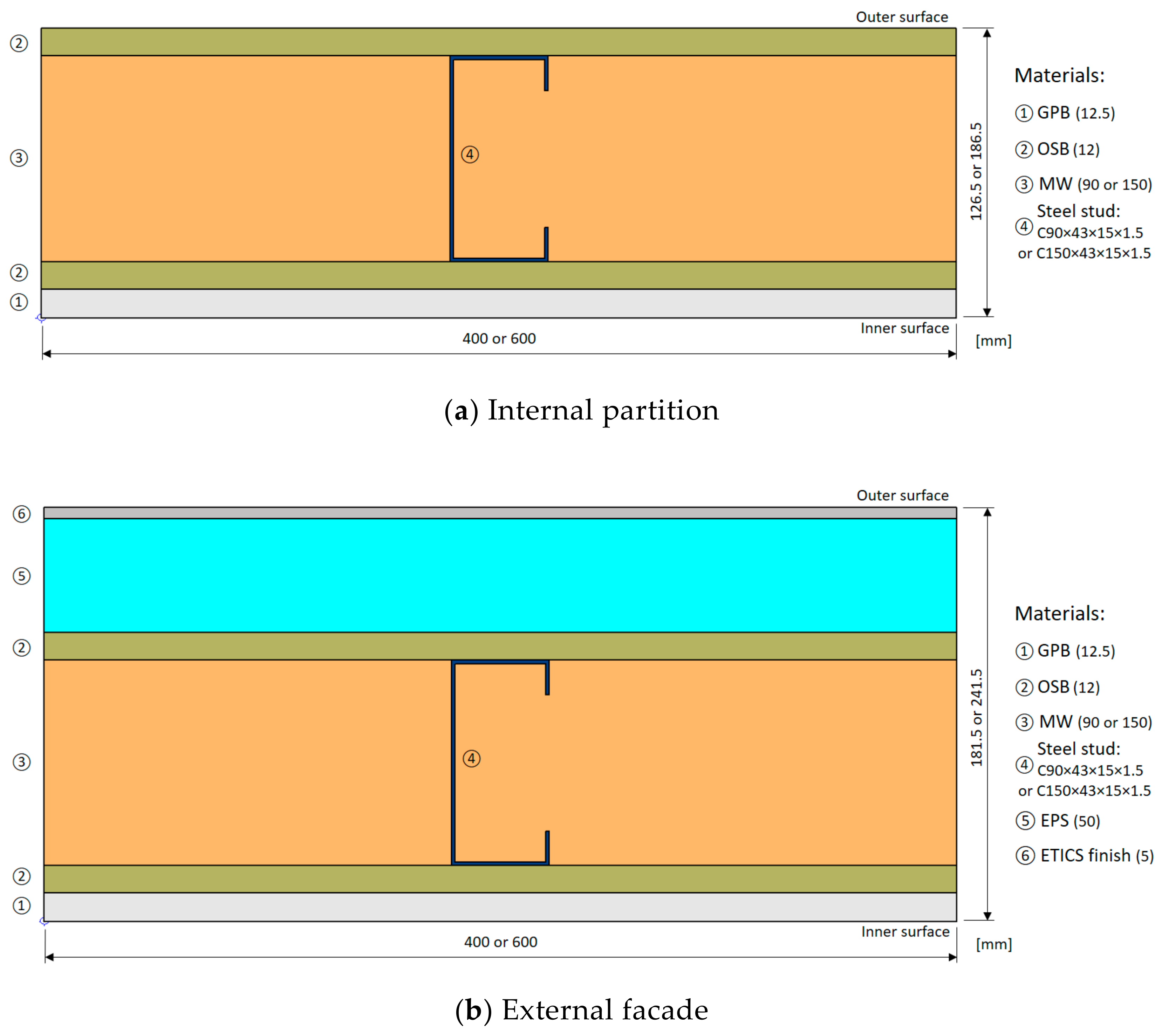
In this work, two reference load-bearing LSF walls were considered, and their cross-sections are illustrated in Figure 1. Both reference LSF walls have structural C-shaped studs with 90 mm thickness (C90), 43 mm flange width, 15 mm lip return with 1.5 mm steel sheet thickness. The 90 mm air gap is filled with mineral wool (MW) batt insulation. On each side of the steel studs there is an oriented strand board (OSB) structural sheathing panel (12 mm thick). In the inner surface there is an additional gypsum plasterboard (GPB) sheathing layer (12.5 mm). The external facade LSF wall has an additional External Thermal Insulation Composite System (ETICS), which consists of an EPS panel (50 mm) and a 5 mm thick finishing layer (Figure 1b).
2.1.2. Evaluated Steel Studs
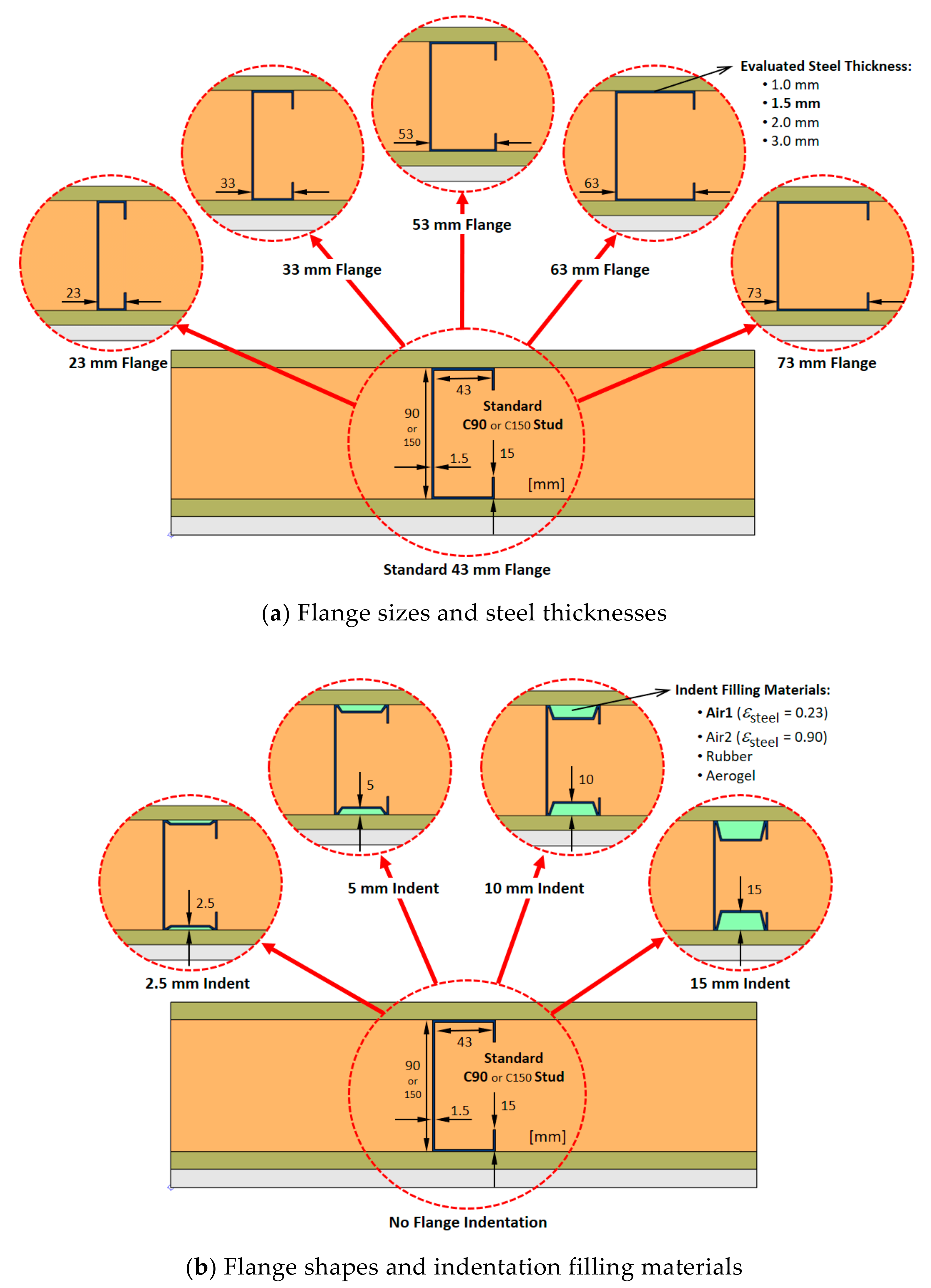
Several steel studs’ configurations were evaluated, as illustrated in Figure 2. Regarding the flange sizes, besides the reference one (43 mm), two smaller (23 and 33 mm) and three larger (53, 63 and 73 mm) sizes were considered (Figure 2a). Moreover, three additional steel sheet thicknesses were considered (1, 2 and 3 mm), besides the reference one (1.5 mm). Concerning the flange shapes, besides the reference one (flat, i.e., without indentation), four additional ones were evaluated, including 2.5, 5, 10 and 15 mm indentation sizes (Figure 2b). Additionally, three indentation filling materials were modeled (rubber, aerogel and air for old dusted steel flanges: ε = 0.90), in addition to the reference one (air for new steel shiny flanges: ε = 0.23). Notice that the illustrations displayed in Figure 2 correspond to load-bearing internal partition LSF walls, but the exterior facade LSF walls have similar steel stud geometry.
2.2. Materials Characterization
The materials used in the LSF walls are listed in Table 2, as well as the thickness of each layer and the corresponding thermal conductivity value. Moreover, Table 3 displays the thermal conductivity of the solid materials used to fill the steel studs’ flange indentations. Regarding emissivity values, a value of 0.90 was assumed for the insulation and sheathing materials [26]. The emissivity adopted for the galvanized cold-formed steel studs was 0.23 [27]. However, to assess the effect of dust accumulation in old steel studs, a higher emissivity value was also modeled, equal to 0.90 [28].
2.3. Numerical Simulations
The finite element method (FEM) software THERM (version 7.6.1) [37] was used to perform the 2D numerical simulations of the LSF walls. The corresponding model details are explained next.
2.3.1. Domain Discretization
To minimize computation time and effort, only a representative bi-dimensional part of the walls’ cross-sections (400 mm or 600 mm width, depending on the studs’ frequency) was modeled, as previously illustrated in Figure 1, for the reference load-bearing LSF walls: (a) internal partition, and (b) external facade, respectively. The thermal properties of the materials used in these simulations were previously presented in Section 2.2 (Table 2 and Table 3). Moreover, the maximum error admitted on the FEM computations was set to 2% for all the models built and assessed in this work.
2.3.2. Boundary Conditions
Two sets of boundary conditions were defined for each THERM model: (1) environment air temperatures, and (2) surface thermal resistances. The warmer interior air temperature was set to 20 °C, while the exterior air temperature was set to 0 °C for the exterior facade wall models. An additional “exterior” temperature of 10 °C was set for the partition walls, assuming an unconditioned space (such as a garage), being that this value was considered an intermediate temperature between the adopted indoor (20 °C) and outdoor (0 °C) temperatures. Nevertheless, the obtained and values do not depend on the chosen temperature difference between the interior and exterior environments, since these values are computed for a unitary temperature difference.
Regarding surface thermal resistances, the values set on ISO 6946 [26] for horizontal heat flow were used, i.e., 0.13 and 0.04 m2∙K/W for internal () and external resistance (), respectively. Notice that for the interior partition walls, internal surface resistances were used in both sides of the partition (i.e., 0.13 m2∙K/W) as recommended by ISO 6946 [26] for unheated spaces.
2.3.3. Modeling Small Unventilated Airspaces
The thermal resistances of the small airspaces inside the indented steel flanges (see Figure 2a) were modelled, making use of a solid-equivalent thermal conductivity computed as prescribed in standard ISO 6946 [26] for unventilated air voids. Notice that the emissivity values of the air voids’ surrounding materials (0.23 for new galvanized steel [27], 0.90 for old dusted steel [28] and 0.90 for OSB [26]) were previously presented in Section 2.2.
2.3.4. Model Accuracy Verifications and Validation
The authors have significant experience with modeling LSF elements [15,16,17,18,20,38] using the THERM software [37], which is a well-known high precision finite element simulator for two-dimensional steady-state heat transfer problems. Nevertheless, several accuracy verifications were performed, as well as an experimental validation.
ISO 10211 Test Cases Verification
The first verification consisted of modeling the two bi-dimensional test cases prescribed in ISO 10211, Annex C [39]. The obtained results were equal to the ones presented in the ISO standard or within the admitted tolerance range (not illustrated here for the sake of brevity, but can be seen in previous research works, such as [15,16,17,20]).
ISO 6946 Analytical Approach Verification
The second verification involved the thermal transmittances’ computation for a simplified LSF wall model assuming homogeneous layers (i.e., neglecting the steel studs). This was performed for the two reference LSF walls illustrated in Figure 1: (a) interior partition, and (b) exterior facade, both with 90 mm of mineral wool filling the air-cavity. The materials’ thermal conductivities and the surface thermal resistances were the ones previously presented in Section 2.2 and Section 2.3.2, respectively. The obtained results are displayed in Table 4. As expected, the analytical ISO 6946 [26] and the numerical results [37] perfectly match for the interior partition and exterior facade walls.
3D FEM Verification
The accuracy of the THERM models was also verified by comparison with 3D models generated in the ANSYS software [40]. Notice that the boundary conditions used in these simulations are in accordance with the laboratory measurements presented in the next subsection, entitled “Lab measurements validation”. Thus, the hot (“interior”) and cold (“exterior”) environment air temperatures were 40 °C and 5 °C, respectively. Moreover, the surface thermal resistances were modeled using the average values measured, taking into account the air and surface temperature differences and the surface heat fluxes. Therefore, the simulated inner () and outer () surface thermal resistances were 0.06 and 0.13 W/(m2∙K), respectively.
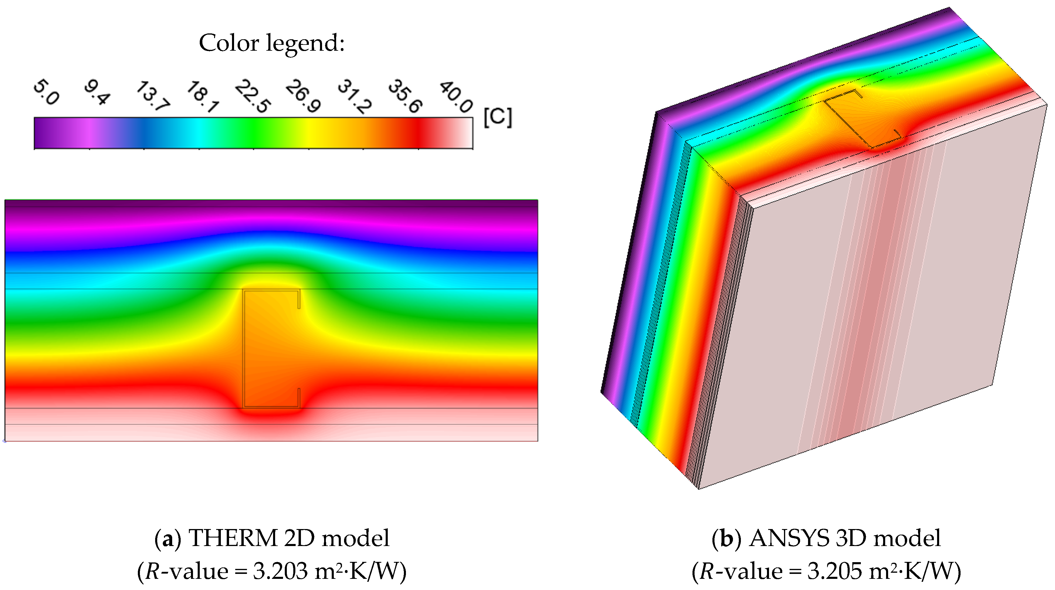
Figure 3 displays the colored temperature distribution for an exterior facade wall model build in: (a) THERM, and (b) ANSYS. The geometry and dimensions were previously illustrated in Figure 1b (C90 × 43 × 15 × 1.5 mm steel studs, which were spaced 400 mm apart), and the thermal conductivity of materials are listed in Table 2. It is well visible in the predicted temperature color distribution, on both 2D and 3D models, the TB effect due to the steel stud’s higher thermal conductivity and consequent increased heat transfer. Moreover, both simulated colored temperature distributions within the horizontal cross-sections of the LSF facade wall are analogous. Furthermore, the obtained surface-to-surface thermal resistances (-values) are very similar, having a very reduced difference, i.e., only 0.002 W/(m2∙K).
Lab Measurements Validation
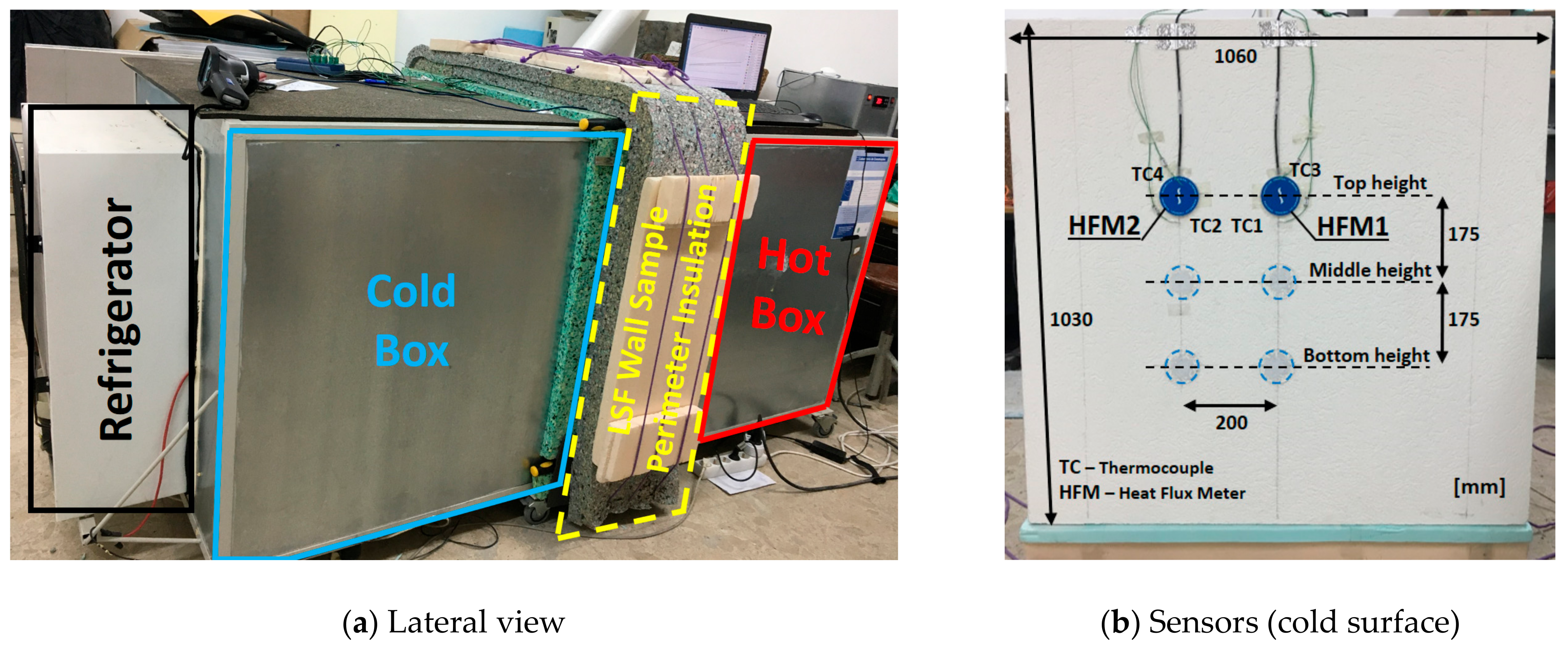
The THERM model was also validated by making use of lab measurements for a small LSF wall test sample (see Figure 4b), which was placed between a hot box (heated by an electrical thermal resistance) and a cold box (cooled by a refrigerator), as illustrated in Figure 4a. To minimize the heat losses through the lateral surfaces of the LSF wall sample, its perimeter was covered by polyurethane foam insulation (80 mm thick).
Four heat flux meters (Hukseflux model HFP01, precision: ±3%) were used, with two on the hot surface and the remaining two on the cold wall surface (Figure 4b). In both wall surfaces (hot and cold), one HFM was located in the vicinity of the vertical steel stud (HFM1) and another one in the middle of the insulation cavity (HFM2), which allow measuring of the two distinct thermal behavior zones within the LSF wall sample. Temperatures were measured using twelve type K (1/0.315) PFA insulated thermocouples (TCs), certified with class one precision. Moreover, these TCs were calibrated in the temperature range [5 °C; 45 °C], with a 5 °C increment, making use of a thermostatic stirring water bath (Heto CB 208), where the TCs were immerged.
Six of the TCs were used for the measurements in the hot side of the tested wall, while another six were used in the cold side. Among the six cold or hot TCs, two measured the environment air temperature inside each box (TC5 and TC6), another two measured the air temperature between the radiation shield and the wall surface (TC3 and TC4), while the remaining two measured the wall surface temperatures (TC1 and TC2), as illustrated in Figure 4b. The temperature and heat flux data measured during the experiments were recorded, making use of two PICO TC-08 data-loggers (precision: ±0.5 °C): one for each side of the LSF wall test-specimen (hot and cold). These data-loggers were connected to a laptop and the software used to manage this data was the PicoLog version 6.1.10.
In these measurements, the heat flow meter (HFM) method was used [41], but with an improvement, as suggested by Rasooli and Itard [42], to increase precision and reduce test duration, i.e., the heat fluxes were measured simultaneously at both hot and cold wall surfaces, instead of measuring on only one side, as prescribed by ISO 9869-1 [41]. The measurements were performed in a quasi-steady-state heat transfer condition and the temperature set-points provided for the hot and cold boxes were 40 °C and 5 °C, respectively.
The convergence criteria prescribed in ASTM C1155–95 [43] were adopted for the “summation technique”, i.e., assuming a maximum admissible convergence factor equal to 10%. Therefore, only the estimated hourly -values with an absolute difference, in relation to the previous time obtained -value, lower than 10% were considered in the measurements. The minimum duration of each measurement test was 24 h.
To ensure the repeatability of the experimental measurements, one test was performed for each wall at three height locations, as illustrated in Figure 4b, that is: (1) top, (2) middle, and (3) bottom, with the average of these three tests being considered the measured overall conductive -value of the LSF wall (Table 5). Making use of the recorded data (heat fluxes and temperatures) for each test and applying the HFM method [41], two distinct conductive local -values were obtained: (1) a lower value for location one (Figure 4b), i.e., in the vicinity of the steel studs (); and (2) a higher value between the steel studs, i.e., in the middle of the insulation cavity (). The overall surface-to-surface -value of the wall () was obtained by computing an area weighted of both measured conductive -values. The steel stud influence area () was defined as prescribed by the ASHRAE zone method [44], i.e., assuming a zone factor (zf) equal to 2.0 [16]. More details about these measurements can be found in reference [21].
Table 5 displays the measured surface-to-surface -values for the three sensor locations (top, middle and bottom, as illustrated in Figure 4b), as well as the corresponding average conductive thermal resistance (3.200 m2∙K/W). This table also shows the conductive -values computed by THERM (Figure 3a) and ANSYS (Figure 3b) FEM models for the LSF facade wall. All these -values are very similar with a small difference regarding the measured thermal resistance: +0.2% for the ANSYS predicted value and +0.1% for THERM. This excellent agreement between the predicted and measured -values allow validating and ensuring the accuracy of the presented THERM models.
Notice that THERM and ANSYS are two of the most well-known state-of-the-art finite elements software. Moreover, THERM has the advantage of being freeware, while ANSYS is a more robust and complete software that allows modeling 3D problems.
3. Obtained Results
In this section, the obtained results are presented. The first set of results are related to the stud flanges’ dimensions for different steel thicknesses, while the second is about the stud flanges’ shape for several indentation filling materials.
3.1. Stud Flanges Size and Steel Thicknesses
To evaluate the importance of the stud flanges’ length in the thermal resistance of LSF walls, 144 models were simulated in THERM software [37], corresponding to three steel frame configurations (i.e., C90 studs, spaced 600 mm; C150 studs, spaced 600 mm, and; C90 studs, spaced 400 mm), six stud flange lengths (i.e., 23, 33, 43 (ref.), 53, 63 and 73 mm), four steel thicknesses (i.e., 1.0, 1.5 (ref.), 2.0 and 3.0 mm) and two LSF wall types (i.e., internal partition and external facade).
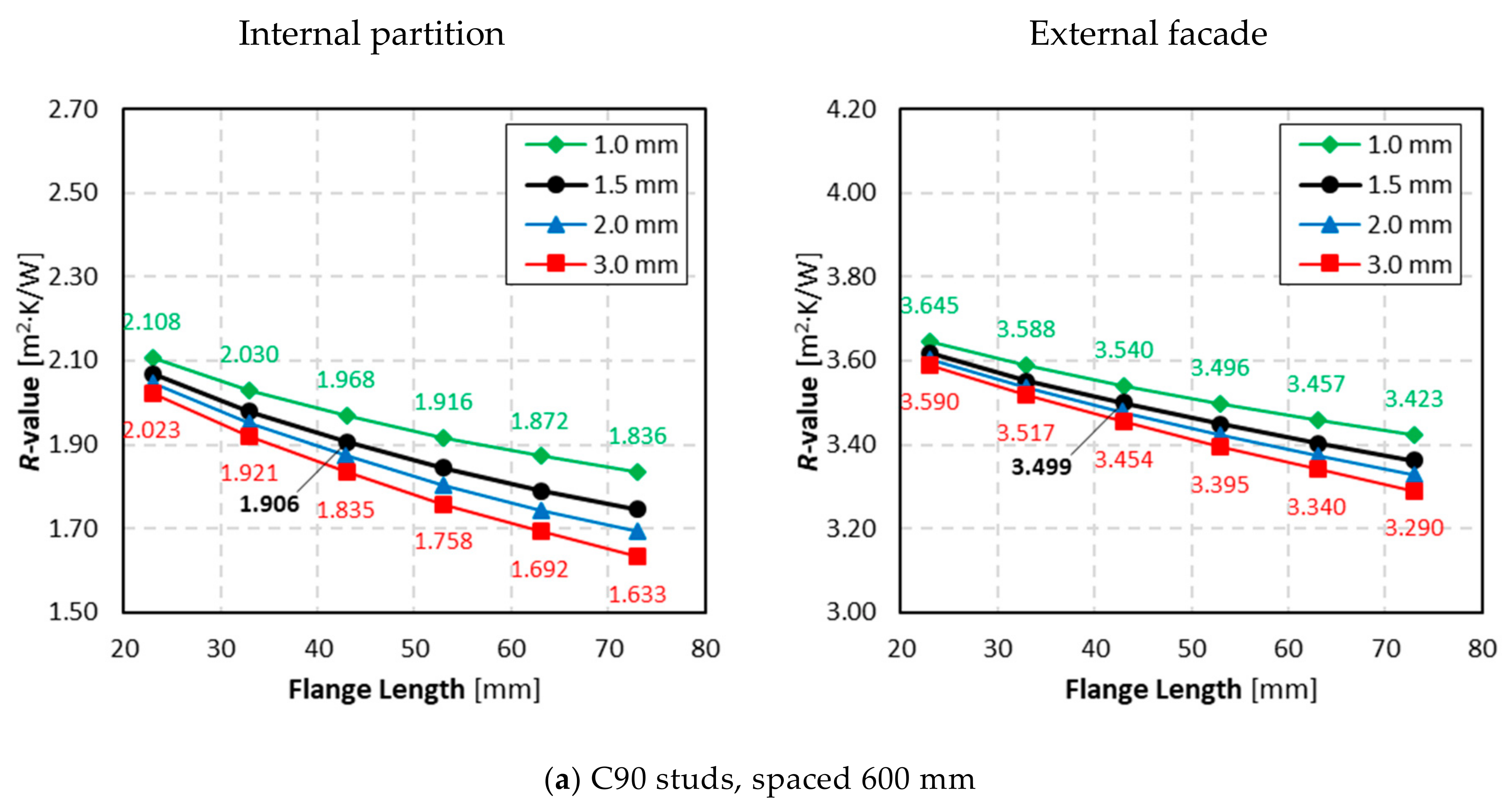
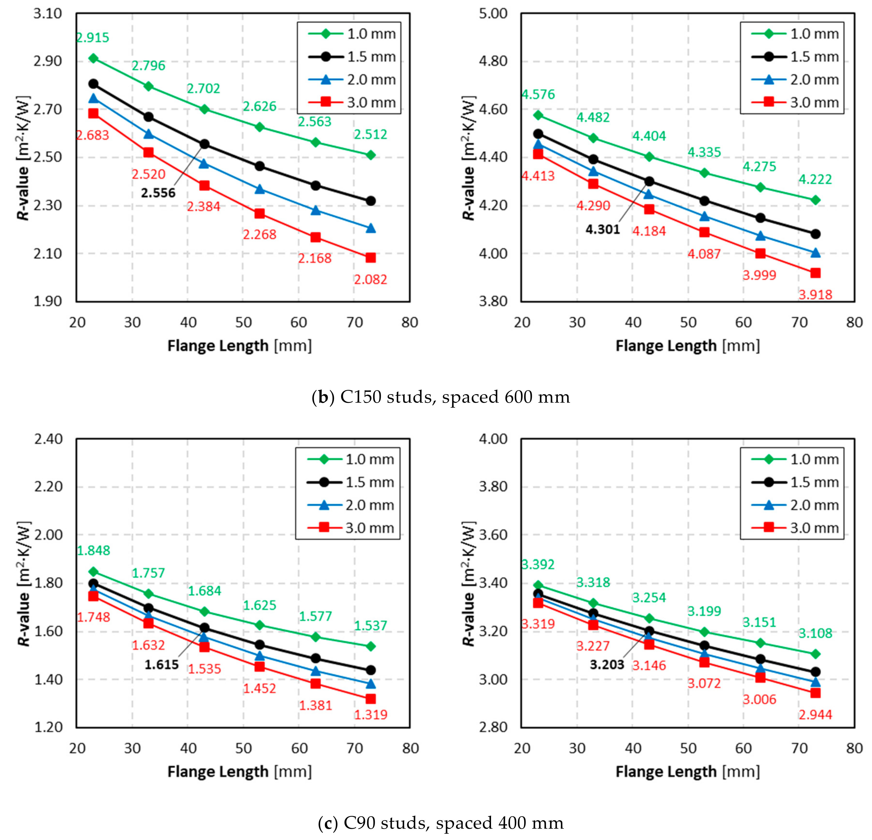
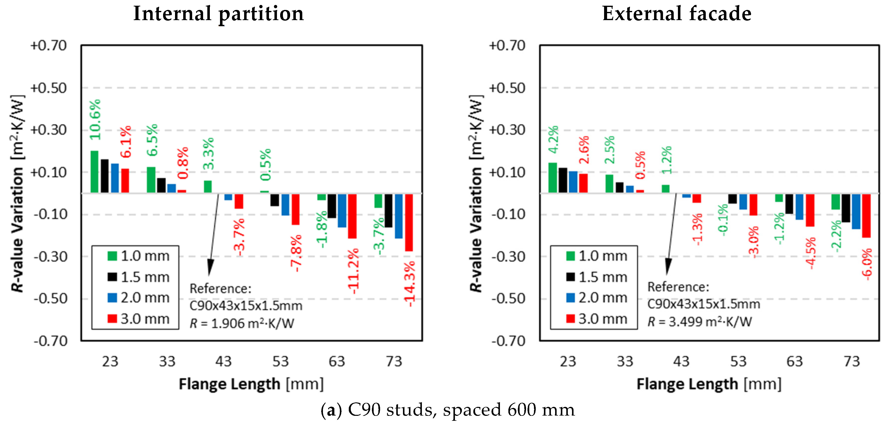
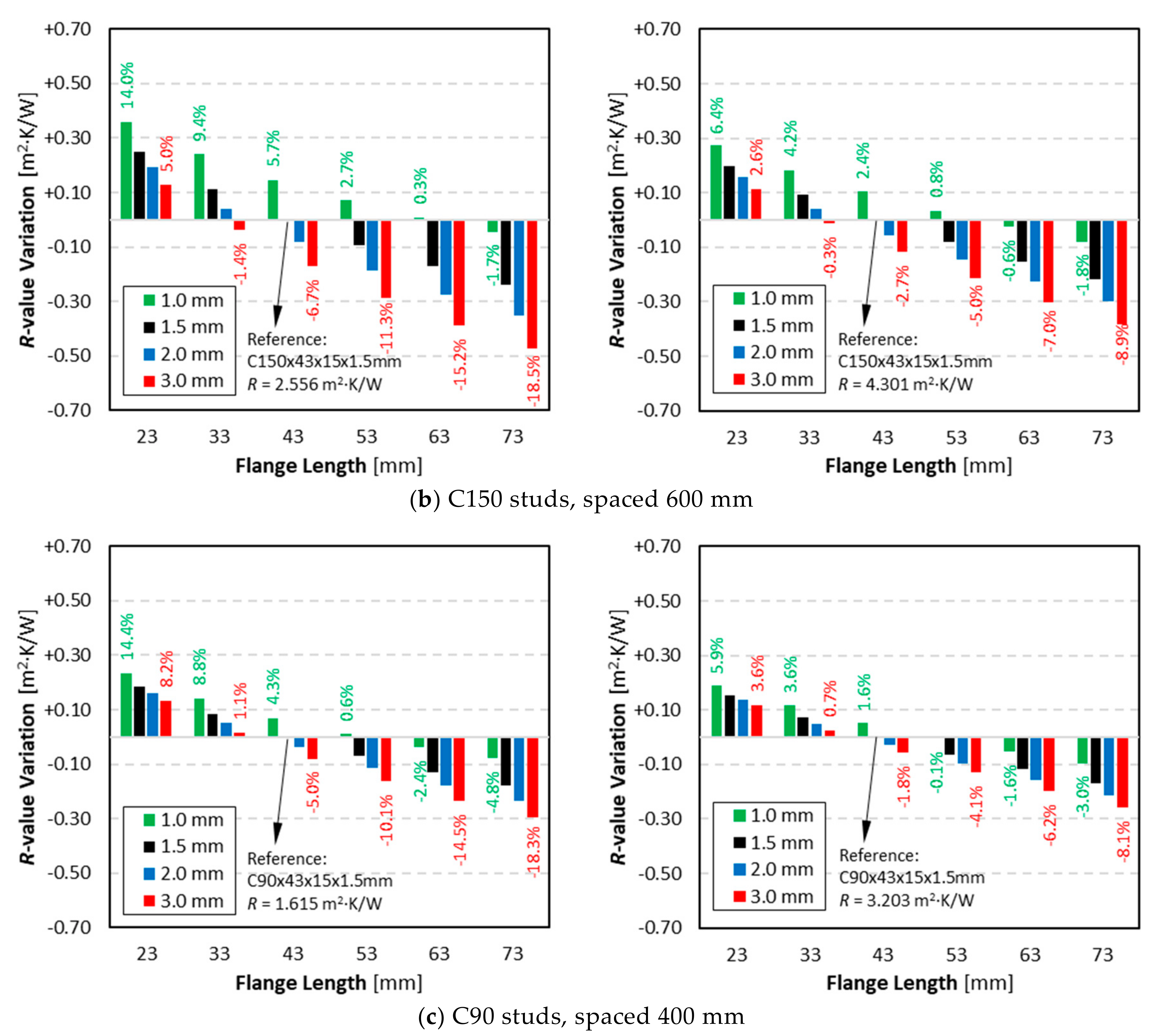
Table 6 displays the obtained surface-to-surface thermal resistance values, while Figure 5 contains a graphical display of these -values. Moreover, Figure 6 illustrates the conductive -value differences for different steel thicknesses and flange lengths, with a standard C-shaped stud for reference, with 1.5 mm thickness and 43 mm flange size. To provide an easier comparison between the several plotted results, the y-axis range in Figure 5 is the same for all graphs (1.2 m2∙K/W). Similarly, for the -value variation in Figure 6, the maximum and minimum y-axis values were fixed at ±0.7 m2∙K/W. Moreover, Figure 7 displays the temperature distribution for LSF walls with different flange lengths, allowing to better understand their influence in the walls’ thermal performance.
3.1.1. Internal Partition
The reference -value for the partition LSF walls with C90 studs spaced 600 mm (43 mm flange length and 1.5 mm steel thickness) is 1.906 m2∙K/W (bold value in Table 6 and left central point in the black line of the left graph of Figure 5a). As expected, the thermal resistance is inversely proportional to the flange length, being minimum (1.745 m2∙K/W) for the maximum evaluated flange length (73 mm), and maximum (2.068 m2∙K/W) for the minimum evaluated flange length (23 mm). This -value variation is not linear, exhibiting a small trend to be more reduced for higher flange lengths (Figure 5a). Moreover, when the steel thickness is reduced to 1.0 mm (green line in Figure 5a), the corresponding -value increase is greater than the -value decrease when steel thickness is augmented to 2.0 mm (blue line). Furthermore, the -value decrease (blue and red lines in Figure 5a) due to the 1.0 mm steel thickness increase (from 2 mm up to 3 mm), is similar to the -value decrease (black and blue lines) due to the mere 0.5 mm steel thickness increase (from 1.5 mm up to 2 mm). Thus, the -value variations are more relevant for smaller steel thicknesses.
When the thickness of the LSF partition wall is increased to 150 mm (Figure 5b), the reference -value is also increased to 2.556 m2∙K/W (Table 6), given the higher amount of mineral wool thermal insulation. Comparing these computed thermal resistance lines in Figure 5b with the previous ones for C90 studs (Figure 5a), two main differences arise, besides the bigger values. One is the greater importance of the flange size in the -value variation, with all the plotted lines being more inclined. Another major difference is the higher separation between the four plotted curves, denoting a higher importance of the steel thickness in the partition wall -values. This greater -value variation is also well visible and quantified in Figure 6b. Looking first to the higher thermal resistance positive variation (23 mm flange length and 1.0 mm steel thickness) for C150 studs (Figure 6b), there is a 0.359 m2∙K/W (+14.0%) R-value increase, while for the previous C90 studs (Figure 6a) this increase was only 0.202 m2∙K/W (+10.6%). Now looking to the higher thermal resistance decrease (73 mm flange length and 3.0 mm steel thickness), i.e., −0.474 m2∙K/W (−18.5%) for C150 studs (Figure 6b), while for the C90 studs (Figure 6a) this -value reduction was only −0.273 m2∙K/W (−14.3%).
Considering, now, the temperature distribution displayed in Figure 7 (left side: internal partition), the relevance of the steel flange dimension is quite visible in the TB effect originated by the steel studs. In fact, for larger steel flanges (Figure 7c), there is a superior temperature perturbation along the LSF wall surfaces in the vicinity of the studs, reducing, in this way, their overall thermal resistance.
When the distance between the steel studs of the LSF partition wall becomes reduced to 400 mm (Figure 5c), the reference -value is also decreased to 1.615 m2∙K/W (Table 6), due to the higher amount of steel per unitary wall length. Now, the trend of the computed -value lines for different steel thicknesses (Figure 5c) are similar to the original ones for C90 studs, spaced 600 mm (Figure 5a). This feature can also be verified in the -value differences plotted in Figure 6c, where, looking to the absolute differences, the values for both studs’ spacing, 600 mm (Figure 6a) and 400 mm (Figure 6c), are quite similar. However, due to different reference -values, looking to the percentage values, the latter ones are bigger.
3.1.2. External Facade
When considering the external facade (i.e., an LSF wall with ETICS) the conductive thermal resistance values become significantly higher (see right side of Table 6, Figure 5 and Figure 6) given the 50 mm thick continuous EPS exterior thermal insulation.
The reference -value for the facade LSF walls with C90 studs spaced 600 mm (43 mm flange length and 1.5 mm steel thick) is 3.499 m2∙K/W (Table 6 and left central point in black line of right chart in Figure 5a). Comparing this external facade plot (right column) with the partition wall (left column), the importance of the steel thickness is now reduced (the four curves are closer) and the relevance of the flange size is also reduced (more linear curves with lower slope). These features are even more visible in Figure 6a, both in absolute -value differences, as well as in percentage variations, now ranging from −6.0% (instead of −10.6%) up to +4.2% (instead of +14.3%), for 3 mm steel thickness with 73 mm flange size and for 1 mm steel thickness with 23 mm flange size, respectively.
Now looking to the LSF facade wall with C150 studs (Figure 5b) the reference -value is increased to 4.301 m2∙K/W. Again, the importance of the steel thickness and flange size are reduced, since the four curves are closer and with lower slopes (Figure 5b right column) in comparison with the partition LSF wall (left column). These features are more perceptible in Figure 6b, not only in absolute -value differences, but also in percentage variations, now ranging from −8.9% (instead of −18.5%) up to +6.4% (instead of +14.0%). The temperature distribution displayed in Figure 7 (right column: external facade), illustrates how the steel flange length affects the TB originated by the steel stud. Moreover, it also illustrates, by comparison with the internal partition temperature distribution (Figure 7 left column plots), how the ETICS is able to mitigate the TB effect, allowing a more uniform temperature along the external surface of the LSF wall.
Finally, considering now the external facade with C90 studs spaced only 400 mm apart, the reference -value is 3.203 m2∙K/W (Table 6). Once more, due to the existence of a continuous thermal insulation layer (ETICS), the relevance of the steel thickness and flange size are reduced, having now four closer curves (one for each steel thickness) with lower slopes (Figure 5c right column) in comparison with the partition LSF wall (left column). These features are even more noticeable in Figure 6c, not only in absolute -value differences, but also in percentage variations, now ranging from −8.1% (instead of −18.3%) up to +5.9% (instead of +14.4%), for 3 mm steel thickness with 73 mm flange size and for 1 mm steel thickness with 23 mm flange size, respectively.
3.2. Stud Flanges Shape and Indentation Filling Materials
In this subsection, the importance of the stud flanges’ shape is assessed for different indentation sizes and filling materials. With this purpose, 102 models were simulated in THERM software [37], corresponding to three steel frame configurations (i.e., C90 studs, spaced 600 mm; C150 studs, spaced 600 mm; and C90 studs, spaced 400 mm), five flange indentation sizes (0, 2.5, 5, 10 and 15 mm), four filling materials (rubber, air1 (i.e., assuming new steel studs), air2 (i.e., assuming old dusted studs) and aerogel) and two LSF wall types (i.e., internal partition and external facade).
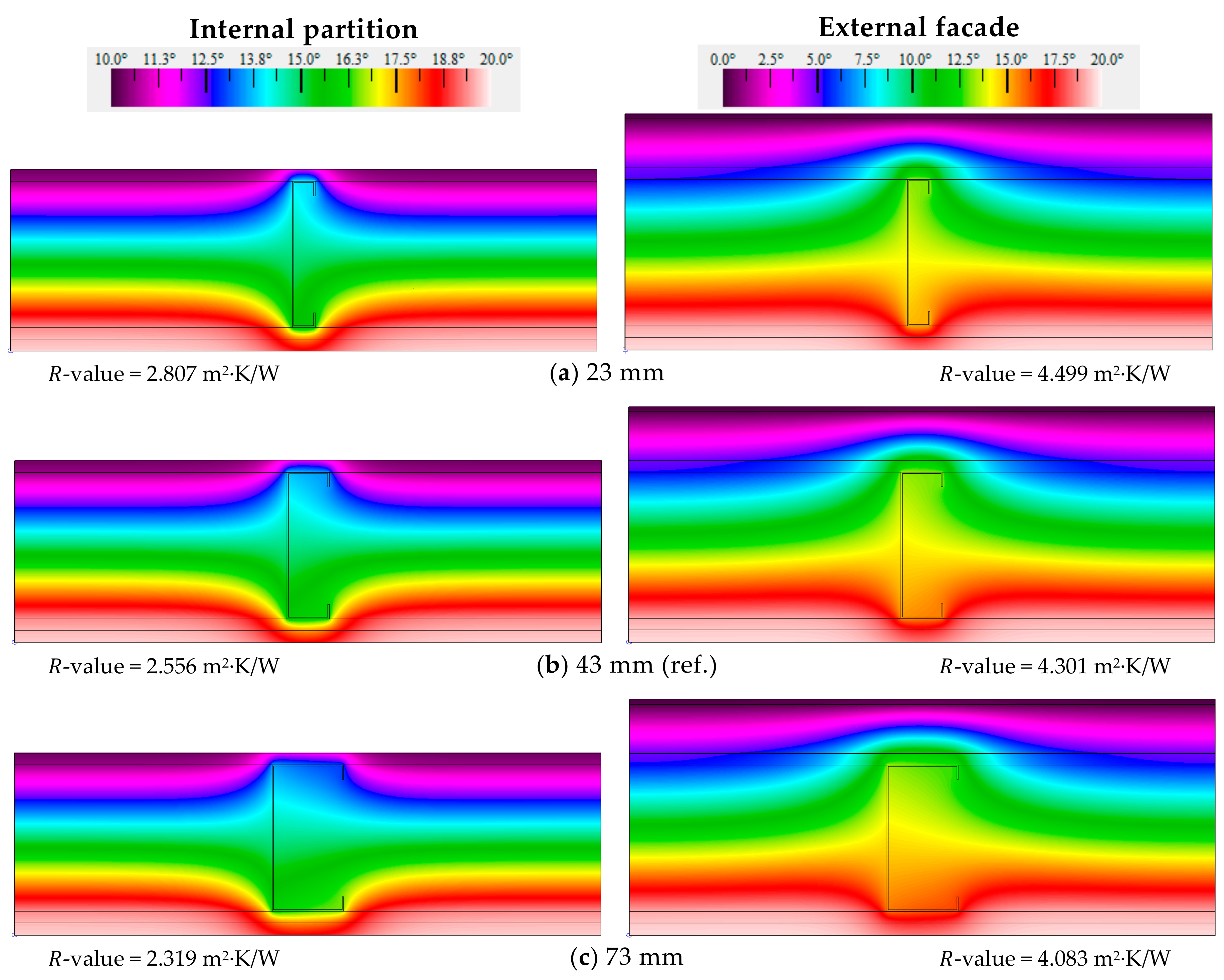
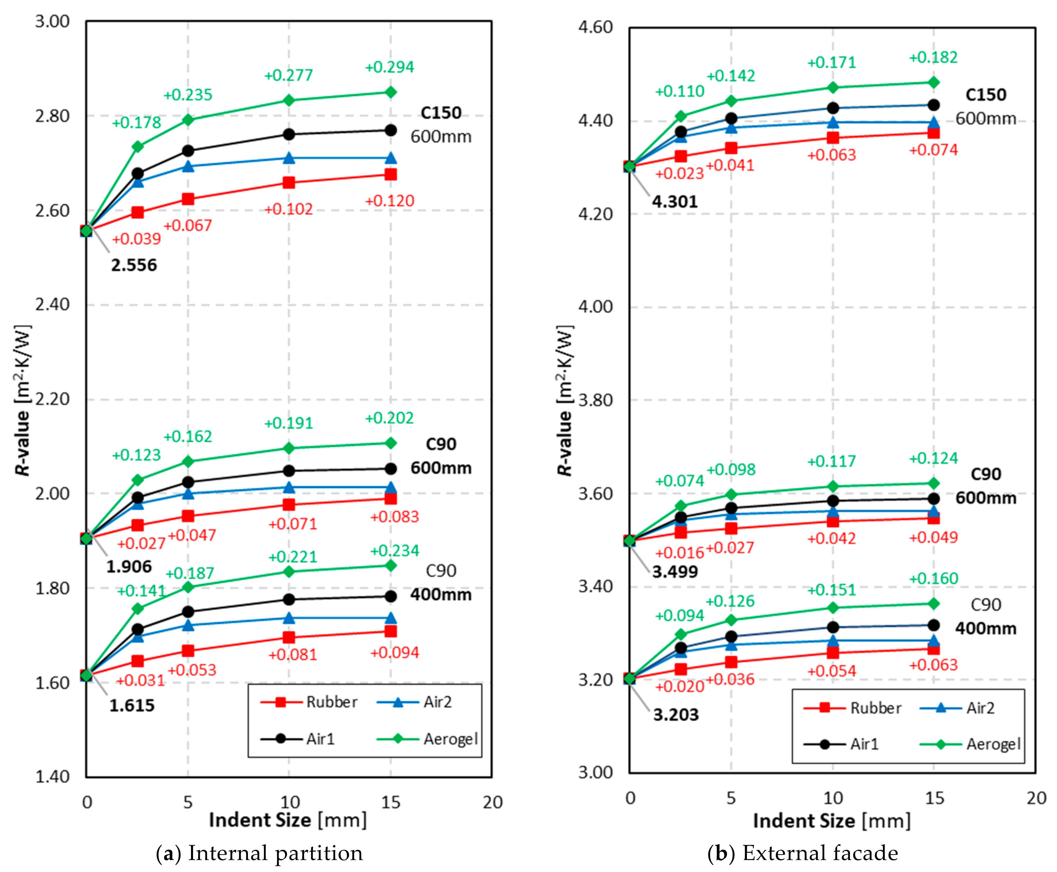
The obtained surface-to-surface thermal resistance values are displayed in Table 7, while Figure 8 contains a graphical display of these conductive -values, as well as the corresponding variations or differences in relation to the reference values, i.e., for standard C-shaped studs with 1.5 mm thickness and 43 mm flange size, without indentation. In the Figure 8 plots, the y-axis range is the same (1.6 m2∙K/W) to provide an easier comparison between the graphics for internal partitions (Figure 8a) and for external facades (Figure 8b). Moreover, to better understand the influence of the stud flange indentation in the LSF walls’ thermal performance, Figure 9 exhibits the temperature distribution for LSF walls with C150 studs spaced 600 mm, with different flange indentations (0, 2.5 and 15 mm) filled with aerogel.
3.2.1. Internal Partition
The reference -value for the partition LSF walls with C90 studs spaced 600 mm with a standard flat flange is 1.906 m2∙K/W (Table 7 and left points in vertical central lines of Figure 8a). As expected, the thermal resistance increases with the indentation size. However, this -value increment is not linear, being higher for smaller indention sizes (e.g., 2.5 mm) and for high performance insulating materials (e.g., aerogel). Analyzing first the black curve (Figure 8a) for new steel studs without any solid filling material (Air1), the initial -value increment (i.e., from 0 to 2.5 mm indentation) is +4.5% (Table 7), while the final one (i.e., from 10 to 15 mm indentation) is only +0.2% (resulting from the difference: 7.7–7.5%). Now looking to the older dusted steel studs (Air2; blue line in Figure 8a), there is quite a similar initial -value increase (+3.9% for 2.5 mm indentation), but for bigger indentation sizes (i.e., from 10 to 15 mm) this increment becomes considerably smaller, converging to 0%. In fact, for the same 15 mm indent size, the thermal resistance for a new steel stud (2.053 m2∙K/W) is higher in comparison with an older dusted one (2.014 m2∙K/W). The rubber indentation filling material curve (in red) is the one that exhibits lower thermal resistance (due to its relative higher thermal conductivity), being the curve more similar to a linear line, exhibiting an almost constant increment trend from smaller to higher indentation sizes. On the other side, the aerogel indentation filling material curve (green color) is the one that provides higher thermal resistances, due to its very reduced thermal conductivity. In this case, the -value increase changes from +6.5% up to +10.6%, having the standard flat steel stud for reference.
For larger steel studs (C150) equally spaced 600 mm apart, the reference -value significantly increased to 2.556 m2∙K/W (Table 7), due to the higher thickness of the mineral wool thermal insulation. As illustrated in Figure 8a, besides a relevant increase in the -values (in comparison with the previous C90 studs set of curves), there is also a larger separation between the four plotted lines, evidencing an increased importance of the steel flanges’ indentation sizes and filling materials. In fact, all of the four lines exhibit a superior relative -value increase. For instance, now the worst performance rubber curve (red line) increment ranges from +0.039 m2∙K/W (+1.5%) up to +0.120 m2∙K/W (+4.7%), while in the C90 stud, it ranged from +0.028 m2∙K/W (+1.5%) up to +0.083 m2∙K/W (+4.4%). A similar trend could be found for the higher performance aerogel green curve, where now the -value increment ranges from +0.178 m2∙K/W (+7.0%) up to +0.294 m2∙K/W (+11.5%), while for the C90 stud, it ranged from +0.123 m2∙K/W (+6.5%) up to +0.202 m2∙K/W (+10.6%).
Looking now to the temperature distribution displayed in Figure 9 (left side: internal partition), the TB mitigation effect originated by the steel flange indention filled with aerogel insulation is quite visible, which is as expected for the larger 15 mm indentation (Figure 9c). This is due to the minimization of the surface contact between the steel flange and the sheathing material (OSB), leading to a lower heat transmission across the LSF wall in the vicinity of the steel studs, increasing, in this way, the global thermal resistance.
To conclude this analysis, the reference -value for the partition LSF with closer C90 steel studs (spaced 400 mm apart) is 1.615 m2∙K/W, which is a relatively reduced value given the higher amount of steel per unitary wall length in comparison with the 600 mm spacing. Comparing this set of four curves with the initial ones (C90 studs spaced 600 mm), there is a very similar trend, but now with a little tendency to show higher -value increments. For example, the rubber red curve exhibits boosts ranging from +0.031 m2∙K/W (+1.9%) up to +0.095 m2∙K/W (+5.9%) and the aerogel green curve shows -value increases ranging from +0.141 m2∙K/W (+8.7%) up to +0.234 m2∙K/W (+14.5%).
3.2.2. External Facade
When there is an ETICS in the LSF wall (i.e., an external facade) the conductive -values are significantly increased (see right side values of Table 7 and Figure 8b) due to the EPS continuous thermal insulation layer (50 mm thick).
The reference -value for the facade LSF walls with C90 studs spaced 600 mm with a standard flat flange is 3.499 m2∙K/W. Once more, the existence of a continuous thermal insulation layer (ETICS) reduces the importance of the flanges’ indentation filling material (the four curves are closer), as well as the relevance of the flange indentation size (more linear curves with lower slope). In fact, for this first set of curves (C90 studs, spaced 600 mm) the -value increment now ranges from +0.049 m2∙K/W (+1.4%) for the rubber (15 mm indentation), up to +0.124 m2∙K/W (+3.5%) for the aerogel filling insulation material (Table 7).
Observing the thicker LSF external facade walls with C150 studs (Figure 8b) the reference -value is significantly increased to 4.301 m2∙K/W, given the higher amount of mineral wool batt insulation. Besides this meaningful -value increase, there is, again, an increased importance of the steel flanges indentation size and filling materials, denoted by the greater separation between the four plotted lines. The worst performance line in red (rubber indentation filling material) now exhibits -value increments ranging from +0.023 m2∙K/W (+0.5%) up to +0.074 m2∙K/W (+1.7%), while the better performance green line (aerogel indentation filling material) ranges from +0.110 m2∙K/W (+2.6%) up to +0.182 m2∙K/W (+4.2%). Regarding the temperature distribution illustrated in Figure 9 (right side: external facade), the steel stud TB effect is visible, as well as their mitigation originated by both ETICS and by the flange indentation filled with aerogel insulation; it is, as expected, larger for the bigger 15 mm indentation (Figure 9c).
Observing now the LSF external facade walls with C90 steel profiles spaced only by 400 mm, the reference R-value is reduced to 3.203 m2∙K/W, with this, as mentioned before, being justified by the higher amount of steel per unitary wall length in comparison with 600 mm spacing. There is a very similar trend between this set of four curves and the initial ones (C90 studs spaced 600 mm), but now with a small tendency to show higher -value increments. For instance, the worst performance rubber red curve exhibits -value increases ranging from +0.020 m2∙K/W (+0.6%) up to +0.063 m2∙K/W (+2.0%), while the best performance aerogel green curve shows -value growths ranging from +0.094 m2∙K/W (+2.9%) up to +0.160 m2∙K/W (+5.0%).
Now, overviewing these obtained results (Table 7, Figure 8 and Figure 9), it can be concluded that use of a steel flange indentation, even a small one (2.5 mm) without any insulation filling material, is useful for increasing the thermal performance of LSF walls, with this benefit being larger for internal partitions in comparison with external facades. Moreover, for the evaluated indentation sizes (up to 15 mm), it is better not to use any filling material rather than to use a poor-performance insulation material, such as rubber. Regarding the adequate indentation size, excluding rubber (which is not worth using), a minimum of 5 mm is recommended, but 10 mm exhibits an acceptable optimum thermal performance improvement, which does not justify an increase to 15 mm, particularly in external facades.
4. Overall Results Discussion
Regarding the previously presented results, the first conclusion remark is that the relevance of the steel stud flange size and indentation is significantly higher for internal partitions than for facade walls due to the existence of an exterior continuous insulation (ETICS) in the latter, which mitigates the steel thermal bridge (TB) effect on the corresponding thermal resistance values.
4.1. Flange Size and Steel Thickness
Concerning the obtained results for the flange size and steel thickness, the main remarks can be summarized as:
- As expected, given the higher amount of steel and the increased steel flange contact surface, the -value of the LSF walls decreases when the flange length and the steel studs’ thickness increases.
- The significance of the flange length and studs’ thickness in the LSF walls’ -values is not linear, being higher for bigger flange sizes and for thicker steel studs.
- The major -value variations for different flange sizes and steel thicknesses occurred for the larger wall thickness, i.e., for C150 studs, due to the higher importance of the steel studs’ TB effect.
- Decreasing the studs’ spacing from 600 mm to 400 mm only originates in a very small increase in the flange size and steel thickness’ importance in the obtained -values, being even more reduced for exterior LSF facade walls.
4.2. Flange Shape and Indentation Filling Materials
Regarding the obtained results for the flange shape and indentation filling materials, the following main remarks could be pointed out:
- As expected, the -value of the LSF walls increases with the increment of the flange indentation size, being that this thermal resistance increase is not linear (i.e., higher variations for lower indentation sizes).
- A small indentation size (2.5 or 5 mm) is enough to provide a significant -value increase, due to the avoidance of the surface contact with the steel flange and a consequent heat transmission reduction.
- The increment in the -value for larger indentation sizes (e.g., from 10 to 15 mm) is very reduced, majorly so for older dusted unfilled steel stud flanges. Therefore, for a long-term perspective, this larger indentation TB mitigation strategy is not recommended.
- The use of indentation filling materials is only beneficial for high performance thermal insulation materials with very small thermal conductivity values (e.g., aerogel).
- For the evaluated indentation sizes (up to 15 mm), the use of low performance insulation materials, such as recycled rubber, is not gainful, since it would be better to leave the stud indentation gap without any solid filling material.
5. Conclusions
In this work, the influence of the stud flanges’ size and shape on the thermal performance of LSF walls was evaluated. Two types of load-bearing LSF walls were studied: (1) internal partition, and (2) exterior facade. Three reference steel studs were considered: (1) C90 spaced 600 mm; (2) C150 spaced 600 mm; and (3) C90 spaced 400 mm. Six stud flange lengths and four steel thicknesses were evaluated, resulting in a total of 144 models. Five flange indentation sizes and four indent filling materials were assessed, corresponding to 102 models. Thus, in this work, a total number of 246 LSF wall models were computed and analyzed. The accuracy of these 2D numerical finite element models was verified by comparison with the ISO standard results and with the 3D FEM predictions; it was also validated by laboratory experimental measurements.
This work allowed for better understanding of the relevance of the stud flanges’ size and shape on the thermal performance of load-bearing LSF internal partitions and external facades. The reference steel studs were commercial ones (C90 and C150) for a flange size of 43 mm. The obtained results enhanced the need for a small indention in the stud flanges (e.g., 2.5 mm). Moreover, using a poor thermal insulation material as a thermal break strip is not advantageous in comparison with keeping an air gap within the indent zone.
Notice that most of the evaluated changes in the steel studs (e.g., flange size and shape, steel thickness) may influence the structural mechanical resistance of load-bearing LSF walls. However, since this work is only focused on the thermal performance, the previously mentioned structural performance variations were not evaluated here.
Author Contributions
Conceptualization, P.S.; methodology, P.S.; validation, P.S.; formal analysis, P.S. and K.P.; investigation, P.S.; writing—original draft preparation, P.S.; writing—review and editing, K.P.; visualization, P.S.; supervision, P.S.; project administration, P.S.; funding acquisition, P.S.. All authors have read and agreed to the published version of the manuscript.
Funding
This research was funded by FEDER funds through the Competitivity Factors Operational Programme—COMPETE and by national funds through FCT—Foundation for Science and Technology within the scope of the project POCI-01-0145-FEDER-032061.

Acknowledgments
The authors also want to thank the support provided by the following companies: Pertecno, Gyptec Ibéria, Volcalis, Sotinco, Kronospan, Hulkseflux, Hilti and Metabo.
Conflicts of Interest
The authors declare no conflict of interest.
References
- European Parliament. Directive (EU) 2018/844 of the European Parliament and of the Council of 30 May 2018 amending Directive 2010/31/EU on the energy performance of buildings and Directive 2012/27/EU on energy efficiency. Off. J. Eur. Union 2018, 156, 75–91. [Google Scholar]
- European Parliament. Directive (EU) 2018/2001 of the European Parliament and of the Council on the promotion of the use of energy from renewable sources. Off. J. Eur. Union 2018, 328, 82–209. [Google Scholar]
- Erhorn-Klutting, H.; Erhorn, H. ASIEPI P148 Impact of thermal bridges on the energy performance of buildings. Build. Platf. Eur. Communities 2009, P148, 1–8. [Google Scholar]
- Theodosiou, T.G.; Papadopoulos, A.M. The impact of thermal bridges on the energy demand of buildings with double brick wall constructions. Energy Build 2008, 40, 2083–2089. [Google Scholar] [CrossRef]
- Al-Sanea, S.A.; Zedan, M.F. Effect of thermal bridges on transmission loads and thermal resistance of building walls under dynamic conditions. Appl. Energy 2012, 98, 584–593. [Google Scholar] [CrossRef]
- Jedidi, M.; Benjeddou, O. Effect of Thermal Bridges on the Heat Balance of Buildings. Int. J. Sci. Res. Civ. Eng. 2018, 2, 41–49. [Google Scholar]
- Zhan, Q.; Xiao, Y.; Musso, F.; Zhang, L. Assessing the hygrothermal performance of typical lightweight steel-framed wall assemblies in hot-humid climate regions by monitoring and numerical analysis. Build. Enviorn. 2021, 188, 107512. [Google Scholar] [CrossRef]
- Soares, N.; Santos, P.; Gervásio, H.; Costa, J.J.; da Silva, L.S. Energy efficiency and thermal performance of lightweight steel-framed (LSF) construction: A review. Renew. Sustain. Energy Rev. 2017, 78, 194–209. [Google Scholar] [CrossRef]
- Santos, P.; da Silva, L.S.; Ungureanu, V. Energy Efficiency of Light-weight Steel-framed Buildings, 1st ed.; Technical Committee 14 Sustainability & Eco-Efficiency of Steel Construction; European Convention for Constructional Steelwork (ECCS): Brussels, Belgium, 2012; ISBN 978-92-9147-105-8. [Google Scholar]
- Varadi, J.; Toth, E. Thermal Improvement of Lightweight Façades containing Slotted Steel Girders. In Twelfth International Conference on Civil, Structural and Environmental Engineering Computing; Civil-Comp Press: Stirlingshire, Scotland, 2009; p. 107. [Google Scholar]
- Lupan, L.M.; Manea, D.L.; Moga, L.M. Improving Thermal Performance of the Wall Panels Using Slotted Steel Stud Framing. Procedia Technol. 2016, 22, 351–357. [Google Scholar] [CrossRef] [Green Version]
- Santos, P.; Martins, C.; da Silva, L.S.; Bragança, L. Thermal performance of lightweight steel framed wall: The importance of flanking thermal losses. J. Build. Phys. 2014, 38, 81–98. [Google Scholar] [CrossRef] [Green Version]
- Martins, C.; Santos, P.; da Silva, L.S. Lightweight steel-framed thermal bridges mitigation strategies: A parametric study. J. Build. Phys. 2016, 39, 342–372. [Google Scholar] [CrossRef]
- Kapoor, D.R.; Peterman, K.D. Quantification and prediction of the thermal performance of cold-formed steel wall assemblies. Structures 2021, 30, 305–315. [Google Scholar] [CrossRef]
- Santos, P.; Lemes, G.; Mateus, D. Thermal Transmittance of Internal Partition and External Facade LSF Walls: A Parametric Study. Energies 2019, 12, 2671. [Google Scholar] [CrossRef] [Green Version]
- Santos, P.; Lemes, G.; Mateus, D. Analytical Methods to Estimate the Thermal Transmittance of LSF Walls: Calculation Procedures Review and Accuracy Comparison. Energies 2020, 13, 840. [Google Scholar] [CrossRef] [Green Version]
- Roque, E.; Santos, P. The Effectiveness of Thermal Insulation in Lightweight Steel-Framed Walls with Respect to Its Position. Buildings 2017, 7, 13. [Google Scholar] [CrossRef] [Green Version]
- Roque, E.; Santos, P.; Pereira, A.C. Thermal and sound insulation of lightweight steel-framed façade walls. Sci. Technol. Built Environ. 2019, 25, 156–176. [Google Scholar] [CrossRef]
- Perera, D.; Poologanathan, K.; Gillie, M.; Gatheeshgar, P.; Sherlock, P.; Nanayakkara, S.M.A.; Konthesingha, K.M.C. Fire performance of cold, warm and hybrid LSF wall panels using numerical studies. Thin-Walled Struct. 2020, 157, 107109. [Google Scholar] [CrossRef]
- Santos, P.; Gonçalves, M.; Martins, C.; Soares, N.; Costa, J.J. Thermal Transmittance of Lightweight Steel Framed Walls: Experimental Versus Numerical and Analytical Approaches. J. Build. Eng. 2019, 25, 100776. [Google Scholar] [CrossRef]
- Santos, P.; Mateus, D. Experimental assessment of thermal break strips performance in load-bearing and non-load-bearing LSF walls. J. Build. Eng. 2020, 32, 101693. [Google Scholar] [CrossRef]
- Atsonios, I.A.; Mandilaras, I.D.; Kontogeorgos, D.A.; Founti, M.A. Two new methods for the in-situ measurement of the overall thermal transmittance of cold frame lightweight steel-framed walls. Energy Build. 2018, 170, 183–194. [Google Scholar] [CrossRef]
- Zalewski, L.; Lassue, S.; Rousse, D.; Boukhalfa, K. Experimental and numerical characterization of thermal bridges in prefabricated building walls. Energy Convers. Manag. 2010, 51, 2869–2877. [Google Scholar] [CrossRef]
- Gomes, A.P.; de Souza, H.A.; Tribess, A. Impact of thermal bridging on the performance of buildings using Light Steel Framing in Brazil. Appl. Eng. 2013, 52, 84–89. [Google Scholar] [CrossRef] [Green Version]
- De Angelis, E.; Serra, E. Light steel-frame walls: Thermal insulation performances and thermal bridges. Energy Procedia 2014, 45, 362–371. [Google Scholar] [CrossRef] [Green Version]
- ISO. ISO 6946. In Building Components and Building Elements Thermal Resistance and Thermal Transmittance Calculation Methods; International Organization for Standardization: Geneva, Switzerland, 2017. [Google Scholar]
- Manzan, M.; de Zorzi, E.Z.; Lorenzi, W. Numerical simulation and sensitivity analysis of a steel framed internal insulation system. Energy Build. 2018, 158, 1703–1710. [Google Scholar] [CrossRef] [Green Version]
- OPTOTHERM Thermal Imaging Materials Emissivity Values. 2020. Available online: www.optotherm.com/emiss-table.htm (accessed on 1 January 2020).
- GYPTEC Ibérica. Technical Sheet: Standard Gypsum Plasterboard (in Portuguese). 2019. Available online: www.gyptec.eu/documentos/Ficha_Tecnica_Gyptec_A.pdf (accessed on 14 March 2019).
- KRONOSPAN OSB. Technical Sheet: KronoBuild OSB 3. 2019. Available online: https://de.kronospan-express.com/public/files/downloads/kronobuild/kronobuild-en.pdf (accessed on 14 March 2019).
- VOLCALIS Mineral Wool. Technical Sheet: Alpha Mineral Wool (in Portuguese). 2019. Available online: www.volcalis.pt/categoria_file_docs/fichatecnica_volcalis_alpharolo-253.pdf (accessed on 14 March 2019).
- ISO. ISO 10456. In Building Materials and Products Hygrothermal Properties Tabulated Design Values and Procedures for Determining Declared and Design Thermal Values; International Organization for Standardization: Geneva, Switzerland, 2007. [Google Scholar]
- TINCOTERM EPS. Technical Sheet: EPS 100 (in Portuguese). 2015. Available online: www.lnec.pt/fotos/editor2/tincoterm-eps-sistema-co-1.pdf (accessed on 14 March 2019).
- WEBERThERM UNO. Technical Sheet: Weber Saint-Gobain ETICS Finish Mortar (in Portuguese). 2018. Available online: www.pt.weber/files/pt/2019-04/FichaTecnica_weberthermuno.pdf (accessed on 14 March 2019).
- ITeCons. Test Report HIG 363/12 Determination of Thermal Resistance; Instituto de Investigação e Desenvolvimento em Ciências da Construção. ITeCons: Coimbra, Portugal, 2012. [Google Scholar]
- SPACETHERM Aerogel. Technical Sheet: Cold Bridge Strip. 2018. Available online: www.proctorgroup.com/assets/Datasheets/Spacetherm_CBS_Datasheet.pdf (accessed on 14 March 2019).
- THERM; Software version 7.6.1; Lawrence Berkeley National Laboratory, United States Department of Energy: San Francisco, CA, USA, 2017. Available online: https://windows.lbl.gov/software/therm (accessed on 14 February 2019).
- Lohmann, V.; Santos, P. Trombe Wall Thermal Behavior and Energy Efficiency of a Light Steel Frame Compartment: Experimental and Numerical Assessments. Energies 2020, 13, 2744. [Google Scholar] [CrossRef]
- ISO. ISO 10211. In Thermal Bridges in Building Construction Heat Flows and Surface Temperatures Detailed Calculations; ISO, International Organization for Standardization: Geneva, Switzerland, 2017. [Google Scholar]
- ANSYS CFX, Software Version 19.1; ANSYS, Inc.: Canonsburg, PA, USA, 2018. Available online: www.ansys.com/products/fluids/ansys-cfx(accessed on 8 January 2020).
- ISO. ISO 9869-1. In Thermal Insulation Building Elements In-Situ Measurement of Thermal Resistance and Thermal Transmittance; Part 1: Heat Flow Meter Method; ISO, International Organization for Standardization: Geneva, Switzerland, 2014. [Google Scholar]
- Rasooli, A.; Itard, L. In-situ characterization of walls’ thermal resistance: An extension to the ISO 9869 standard method. Energy Build. 2018, 179, 374–383. [Google Scholar] [CrossRef]
- ASTM C1155–95. Standard Practice for Determining Thermal Resistance of Building Envelope Components from the In-Situ Data; ASTM American Society for Testing and Materials: Philadelphia, PA, USA, 2013. [Google Scholar]
- ASHRAE. Handbook of Fundamentals (SI Edition); ASHRAE American Society of Heating; Refrigerating and Air-conditioning Engineers: Atlanta, GA, USA, 2017. [Google Scholar]
Figure 1.
Reference load-bearing LSF walls.

Figure 2.
Geometry of the evaluated steel studs.

Figure 3.
Accuracy verification of the LSF external facade model: Colored temperature distribution and surface-to-surface computed thermal resistances (-value).
Figure 3.
Accuracy verification of the LSF external facade model: Colored temperature distribution and surface-to-surface computed thermal resistances (-value).

Figure 4.
Mini hot box apparatus used for the -value lab measurements.

Figure 5.
LSF walls conductive thermal resistances for different steel thicknesses and flange lengths.
Figure 5.
LSF walls conductive thermal resistances for different steel thicknesses and flange lengths.


Figure 6.
LSF walls conductive thermal resistance variation for different steel thicknesses and flange lengths.
Figure 6.
LSF walls conductive thermal resistance variation for different steel thicknesses and flange lengths.


Figure 7.
Temperature distribution and conductive thermal resistances for LSF walls with C150 studs, 1.5 mm steel thickness, spaced 600 mm, with different flange lengths.
Figure 7.
Temperature distribution and conductive thermal resistances for LSF walls with C150 studs, 1.5 mm steel thickness, spaced 600 mm, with different flange lengths.

Figure 8.
Conductive thermal resistance of three LSF walls with standard “C” shaped studs and their relative variations for different flange indentation sizes and filling materials.
Figure 8.
Conductive thermal resistance of three LSF walls with standard “C” shaped studs and their relative variations for different flange indentation sizes and filling materials.

Figure 9.
Temperature distribution and conductive thermal resistances for LSF walls with C150 studs spaced 600 mm, with different flange indentations filled with aerogel.
Figure 9.
Temperature distribution and conductive thermal resistances for LSF walls with C150 studs spaced 600 mm, with different flange indentations filled with aerogel.


Table 1.
Evaluated load-bearing lightweight steel framed (LSF) walls, reference steel studs, stud flanges sizes and shapes.
Table 1.
Evaluated load-bearing lightweight steel framed (LSF) walls, reference steel studs, stud flanges sizes and shapes.
| Parameter | Values/Description | |
|---|---|---|
| Load-Bearing LSF Walls | Internal Partition (without ETICS 3) | |
| External Facade (with ETICS 3) | ||
| Spacing [mm] | ||
| Reference Steel Studs [mm] | C90 × 43 × 15 × 1.5 | 600 |
| C150 × 43 × 15 × 1.5 | 600 | |
| C90 × 43 × 15 × 1.5 | 400 | |
| Stud Flange Sizes and Steel Thicknesses: | ||
| Stud Flange Length [mm] | 23, 33, 43 *, 53, 63, 73 | |
| Steel Thicknesses [mm] | 1.0, 1.5 *, 2.0, 3.0 | |
| Stud Flange Shapes and Filling Materials: | ||
| Flange Indent Dimension [mm] | 0 *, 2.5, 5, 10, 15 | |
| Indent Filling Materials | Air1 *,1, Air2 2, Rubber, Aerogel | |
* Reference values; ε—Emissivity; 1 Air1—Assuming ε = 0.23 (new steel studs); 2 Air2—Assuming ε = 0.90 (old, dusted studs); 3 ETICS—External Thermal Insulation Composite System.
Table 2.
Thickness ()
and thermal conductivity () of the materials used in the LSF walls.
| Material (Inner to Outer Layer) | d [mm] | [W/(m·K)] | Ref. |
|---|---|---|---|
| GPB 1 | 12.5 | 0.175 | [29] |
| OSB 2 | 12 | 0.100 | [30] |
| MW 3 | 90, 150 | 0.035 | [31] |
| Steel studs | C90, C150 | 50.000 | [32] |
| OSB 4 | 12 | 0.100 | [30] |
| EPS 5 | 50 | 0.036 | [33] |
| ETICS 6 finish | 5 | 0.450 | [34] |
1 GPB—Gypsum Plaster Board; 2 OSB—Oriented Strand Board; 3 MW—Mineral Wool; 4 OSB—Oriented Strand Board; 5 EPS—Expanded Polystyrene; 6 ETICS—External Thermal Insulation Composite System.
Table 3.
Thermal conductivity of flanges’ indentation solid filling materials.
| Material | λ [W/(m·K)] | Ref. |
|---|---|---|
| Recycled rubber | 0.122 | [35] |
| Aerogel | 0.015 | [36] |
Table 4.
Thermal transmittance obtained for simplified wall models with homogeneous layers.
| Wall | -Value [W/(m2·K)] | |
|---|---|---|
| Analytical (ISO 6946) | Numerical (THERM) | |
| Interior partition | 0.318 | 0.318 |
| Exterior facade | 0.225 | 0.225 |
Table 5.
LSF facade wall conductive thermal resistance values measured in lab and computed by 2D (THERM) and 3D (ANSYS) finite element method (FEM) numerical simulations.
Table 5.
LSF facade wall conductive thermal resistance values measured in lab and computed by 2D (THERM) and 3D (ANSYS) finite element method (FEM) numerical simulations.
| Test | Sensors Location | -Value [m2∙K/W] |
|---|---|---|
| 1 | Top | 3.232 |
| 2 | Middle | 3.121 |
| 3 | Bottom | 3.247 |
| Average Measured | 3.200 | |
| Computed by ANSYS | 3.205 | |
| Percentage Deviation | +0.2% | |
| Computed by THERM | 3.203 | |
| Percentage Deviation | +0.1% |
Table 6.
LSF walls conductive thermal resistance [m2∙K/W] for different steel thicknesses and flange lengths.
Table 6.
LSF walls conductive thermal resistance [m2∙K/W] for different steel thicknesses and flange lengths.
| LSF Wall | Flange | Internal Partition | External Facade | ||||||
|---|---|---|---|---|---|---|---|---|---|
| Length | Steel Thickness [mm] | ||||||||
| [mm] | 1.0 | 1.5 * | 2.0 | 3.0 | 1.0 | 1.5 * | 2.0 | 3.0 | |
| C90 studs spaced 600 mm | 23 | 2.108 M | 2.068 | 2.046 | 2.023 | 3.645 M | 3.619 | 3.605 | 3.590 |
| 33 | 2.030 | 1.979 | 1.951 | 1.921 | 3.588 | 3.552 | 3.536 | 3.517 | |
| 43 * | 1.968 | 1.906 * | 1.872 | 1.835 | 3.540 | 3.499 * | 3.477 | 3.454 | |
| 53 | 1.916 | 1.844 | 1.803 | 1.758 | 3.496 | 3.449 | 3.423 | 3.395 | |
| 63 | 1.872 | 1.790 | 1.743 | 1.692 | 3.457 | 3.402 | 3.373 | 3.340 | |
| 73 | 1.836 | 1.745 | 1.692 | 1.633 m | 3.423 | 3.362 | 3.328 | 3.290 m | |
| C150 studs spaced 600 mm | 23 | 2.915 M | 2.807 | 2.747 | 2.683 | 4.576 M | 4.499 | 4.457 | 4.413 |
| 33 | 2.796 | 2.668 | 2.597 | 2.520 | 4.482 | 4.392 | 4.343 | 4.290 | |
| 43 * | 2.702 | 2.556 * | 2.474 | 2.384 | 4.404 | 4.301 * | 4.245 | 4.184 | |
| 53 | 2.626 | 2.463 | 2.370 | 2.268 | 4.335 | 4.221 | 4.156 | 4.087 | |
| 63 | 2.563 | 2.384 | 2.281 | 2.168 | 4.275 | 4.148 | 4.076 | 3.999 | |
| 73 | 2.512 | 2.319 | 2.206 | 2.082 m | 4.222 | 4.083 | 4.004 | 3.918 m | |
| C90 studs spaced 400 mm | 23 | 1.848 M | 1.800 | 1.775 | 1.748 | 3.392 M | 3.357 | 3.339 | 3.319 |
| 33 | 1.757 | 1.698 | 1.666 | 1.632 | 3.318 | 3.275 | 3.251 | 3.227 | |
| 43 * | 1.684 | 1.615 * | 1.576 | 1.535 | 3.254 | 3.203 * | 3.175 | 3.146 | |
| 53 | 1.625 | 1.545 | 1.500 | 1.452 | 3.199 | 3.140 | 3.107 | 3.072 | |
| 63 | 1.577 | 1.487 | 1.436 | 1.381 | 3.151 | 3.084 | 3.046 | 3.006 | |
| 73 | 1.537 | 1.438 | 1.381 | 1.319 m | 3.108 | 3.032 | 2.990 | 2.944 m | |
* Reference values; M Maximum values; m Minimum values.
Table 7.
Conductive thermal resistance of LSF walls with standard “C” shaped studs and their percentage variation for different flange indentation sizes and filling materials.
Table 7.
Conductive thermal resistance of LSF walls with standard “C” shaped studs and their percentage variation for different flange indentation sizes and filling materials.
| LSF Wall | Indent | Internal Partition | External Facade | ||||||
|---|---|---|---|---|---|---|---|---|---|
| Size | Indent Filling Material | ||||||||
| [mm] | Rubber | Air 2 | Air 1 | Aerogel | Rubber | Air 2 | Air 1 | Aerogel | |
| C90 studs spaced 600 mm | 0 | -value * = 1.906 m2∙K/W | -value * = 3.499 m2∙K/W | ||||||
| 2.5 | 1.933 | 1.980 | 1.992 | 2.029 | 3.515 | 3.542 | 3.550 | 3.573 | |
| +1.4% | +3.9% | +4.5% | +6.5% | +0.5% | +1.2% | +1.5% | +2.1% | ||
| 5 | 1.953 | 2.002 | 2.025 | 2.068 | 3.526 | 3.555 | 3.570 | 3.597 | |
| +2.5% | +5.0% | +6.2% | +8.5% | +0.8% | +1.6% | +2.0% | +2.8% | ||
| 10 | 1.977 | 2.014 | 2.048 | 2.097 | 3.541 | 3.563 | 3.584 | 3.616 | |
| +3.7% | +5.7% | +7.5% | +10.0% | +1.2% | +1.8% | +2.4% | +3.3% | ||
| 15 | 1.989 | 2.014 | 2.053 | 2.108 | 3.548 | 3.563 | 3.588 | 3.623 | |
| +4.4% | +5.7% | +7.7% | +10.6% | +1.4% | +1.8% | +2.5% | +3.5% | ||
| C150 studs spaced 600 mm | 0 | -value * = 2.556 m2∙K/W | -value * = 4.301 m2∙K/W | ||||||
| 2.5 | 2.595 | 2.661 | 2.679 | 2.734 | 4.324 | 4.365 | 4.377 | 4.411 | |
| +1.5% | +4.1% | +4.8% | +7.0% | +0.5% | +1.5% | +1.8% | +2.6% | ||
| 5 | 2.623 | 2.693 | 2.727 | 2.791 | 4.342 | 4.385 | 4.406 | 4.443 | |
| +2.6% | +5.4% | +6.7% | +9.2% | +1.0% | +2.0% | +2.4% | +3.3% | ||
| 10 | 2.658 | 2.711 | 2.761 | 2.833 | 4.364 | 4.396 | 4.428 | 4.472 | |
| +4.0% | +6.1% | +8.0% | +10.8% | +1.5% | +2.2% | +3.0% | +4.0% | ||
| 15 | 2.676 | 2.712 | 2.770 | 2.850 | 4.375 | 4.397 | 4.434 | 4.483 | |
| +4.7% | +6.1% | +8.4% | +11.5% | +1.7% | +2.2% | +3.1% | +4.2% | ||
| C90 studs spaced 400 mm | 0 | -value * = 1.615 m2∙K/W | -value * = 3.203 m2∙K/W | ||||||
| 2.5 | 1.646 | 1.698 | 1.713 | 1.756 | 3.223 | 3.259 | 3.268 | 3.297 | |
| +1.9% | +5.1% | +6.1% | +8.7% | +0.6% | +1.7% | +2.0% | +2.9% | ||
| 5 | 1.668 | 1.723 | 1.750 | 1.802 | 3.239 | 3.275 | 3.294 | 3.329 | |
| +3.3% | +6.7% | +8.4% | +11.6% | +1.1% | +2.2% | +2.8% | +3.9% | ||
| 10 | 1.696 | 1.738 | 1.777 | 1.836 | 3.257 | 3.285 | 3.312 | 3.354 | |
| +5.0% | +7.6% | +10.0% | +13.7% | +1.7% | +2.6% | +3.4% | +4.7% | ||
| 15 | 1.709 | 1.737 | 1.784 | 1.849 | 3.266 | 3.285 | 3.317 | 3.363 | |
| +5.8% | +7.6% | +10.5% | +14.5% | +2.0% | +2.6% | +3.6% | +5.0% | ||
* Reference values; 1 Assuming ε = 0.23 (new steel studs); 2 Assuming ε = 0.90 (old, dusted studs).
Publisher’s Note: MDPI stays neutral with regard to jurisdictional claims in published maps and institutional affiliations. |
© 2021 by the authors. Licensee MDPI, Basel, Switzerland. This article is an open access article distributed under the terms and conditions of the Creative Commons Attribution (CC BY) license (https://creativecommons.org/licenses/by/4.0/).
Share and Cite
MDPI and ACS Style
Santos, P.; Poologanathan, K. The Importance of Stud Flanges Size and Shape on the Thermal Performance of Lightweight Steel Framed Walls. Sustainability 2021, 13, 3970. https://0-doi-org.brum.beds.ac.uk/10.3390/su13073970
AMA Style
Santos P, Poologanathan K. The Importance of Stud Flanges Size and Shape on the Thermal Performance of Lightweight Steel Framed Walls. Sustainability. 2021; 13(7):3970. https://0-doi-org.brum.beds.ac.uk/10.3390/su13073970
Chicago/Turabian StyleSantos, Paulo, and Keerthan Poologanathan. 2021. "The Importance of Stud Flanges Size and Shape on the Thermal Performance of Lightweight Steel Framed Walls" Sustainability 13, no. 7: 3970. https://0-doi-org.brum.beds.ac.uk/10.3390/su13073970
Note that from the first issue of 2016, this journal uses article numbers instead of page numbers. See further details here.