
A Regional Approach for Investigation of Temporal Precipitation Changes


Civil Engineering Department, Mugla Sıtkı Kocman University, Mugla 48000, Turkey
Sustainability 2021, 13(10), 5733; https://0-doi-org.brum.beds.ac.uk/10.3390/su13105733
Submission received: 19 March 2021
/
Revised: 11 May 2021
/
Accepted: 11 May 2021
/
Published: 20 May 2021
Abstract
:Climatic variability is one of the fundamental aspects of the climate. Our scope of knowledge of this variability is limited by unavailable long-term high-resolution spatial data. Climatic simulations indicate that warmer climate increases extreme precipitations but decreases high-frequency temperature variability. As an important climatologic variable, the precipitation is reported by the IPCC to increase in mid and high altitudes and decrease in subtropical areas. On a regional scale, such a change needs spatio-parametric justification. In this regard, a regionalization approach relying on frequency characteristics and parameters of heavy precipitation may provide better insight into temporal precipitation changes, and thus help us to understand climatic variability and extremes. This study introduces the “index precipitation method”, which aims to define hydrologic homogeneous regions throughout which the frequency distribution of monthly maximum hourly precipitations remains the same and, therefore, investigate whether there are significant temporal precipitation changes in these regions. Homogenous regions are defined based on L-moment ratios of frequency distributions via cluster analysis and considering the spatial contiguity of gauging sites via GIS. Regarding the main hydrologic characteristics of heavy precipitation, 12 indices are defined in order to investigate the existence of regional trends by means of t- and Mann–Kendall tests for determined homogenous regions with similar frequency behaviors. The case study of Japan, using hourly precipitation data on 150 gauges for 1991–2010, shows that trends that statistically exist for single-site observations should be regionally proved. Trends of heavy precipitation have region-specific properties across Japan. Homogenous regions beneficially define statistically significant trends for heavy precipitation.
1. Introduction
Climatic variability has been recognized as an important problem causing fundamental changes to human life, as well as the natural environment [1,2]. In order to address how this variability has developed and will affect available water resources, one of the main climatologic quantities needing to be investigated is precipitation [3,4,5,6]. Considering the possible effects of climate change on precipitation, many researchers have analyzed and tested the existence of trends in precipitation using basic statistics and updated data for different parts of the world [7,8,9]. Although these studies support, on a global scale, the IPCC report [10,11,12], claiming that precipitation is set to increase in the Northern Hemisphere, mid and high latitudes, but to decrease in subtropical land areas [13] on a local/regional scale, their results are generally of high spatial variation and lack areal support from vicinity sites. In fact, the consistency of calculated hydrologic trends cannot be realistically determined solely by using single-site observations, due to the biases resulting from data-related problems. This problem is more pronounced for the analyses relying on average statistics [14], since average statistics are not highly sensitive to climatic variability [15,16]. Considering that societies and ecosystems are indeed much more vulnerable to extremes compared to averages, a regional approach based on the regional frequency behavior of heavy precipitations and a regional trend indicator based on the multitude of trend indices relying on the basic characteristics of heavy precipitation will be more helpful to verify the existence and consistency of a regional trend of precipitation. This should provide better insight into temporal precipitation changes, as well as climatic variability and extremes.
There are many approaches in the literature for the investigation of the spatial pattern of rainfall, relying on mathematical transformations, statistical regressions, or clustering techniques, such as multivariate regression, spatial interpolation, spatial correlation, harmonic analysis, L-moments, principal component analysis, hierarchical and non-hierarchical clustering techniques [17,18,19]. These approaches use basic basin physiographic and climatic properties for defining the rainfall pattern in a considered area and have been studied by many researchers to obtain a robust methodology that can be applied within a defined homogenous region [20,21,22,23]. One of the eminent methodologies in the literature is the index flood method [24,25]. The index flood method derives homogeneous regions based on regional frequency behaviors and uses local statistics to obtain scaled estimations. Therefore, it preserves both the regional frequency behavior and local statistics of observations within the boundary of the homogenous region. It assumes a common dimensionless regional frequency curve along the homogenous region. The product of this regional frequency curve and the index flood, which is generally taken as the mean of the station data, yields an at-site frequency curve for a considered flow section. Since this method is first developed for flood estimations, it is known as the index flood method [18,24]. On the other hand, ordinary clustering approaches directly use site-specific basin or climatic parameters to define homogenous regions; therefore, such classification approaches are generally quite sensitive to the parameters selected and data used and may not be appropriate for the estimation of spatio-temporal trends in such classified regions.
A homogeneous region is defined in such a way that frequency distributions of monthly maximum hourly precipitations statistically identical throughout the region can more realistically reveal temporal changes in heavy precipitations. This will eliminate difficulties with single-site observations, such as the non-existence of long-term data, differences in observation periods, and inhomogeneous data. Heavy precipitation trend indices on such homogenous regions and thereby a regional trend indicator based on these indices will expose a more realistic picture of a study area for the existence of a significant, consistent trend. This study presents the index precipitation method to define hydrologic homogeneous regions and, therefore, to investigate temporal changes on heavy precipitation. In the example of Japan, homogenous regions were delineated so as to get similar frequency behaviors throughout each homogenous region. L-moment estimations of frequency distributions were used for this purpose, since L-moments produce unbiased frequency distributions and are less sensitive to outliers, making analyses of multi-site observations easier. Thereafter, regions with a similar frequency behavior—homogenous regions—were determined using L-moment ratios diagrams. This was achieved by cluster analysis, classifying gauging sites with the same theoretical distribution and then with similar L-moment ratios. Finally, a geographical information system analysis was implemented to differentiate noncontiguous homogenous classes, or more specifically, to get homogenous regions. Regional trends in these regions were then investigated using different precipitation indices, as well as the regional trend index.
2. Study Area and Data
Hourly precipitations from the Japan Meteorological Agency for the period 1991–2010 are used in the analyses. Records of 150 stations, for which consistent and continuous observations are available, are organized in a visual basic environment in order to obtain continuous hourly time series of precipitation records. These time series of single-site records are used in regional trend analyses in order to determine the spatio-temporal pattern of heavy precipitations throughout Japan. Figure 1 shows the locations and spatial distribution of the stations.
The Japan Meteorological Agency digitized precipitation data in 2000, for the full period of operation, which go back to 1900 for some sites [3]. Using annual data, the Japan Meteorological Agency [26] found a slightly decreasing trend in precipitation for the last century. There are also some researches testing long-term trends in hourly, daily, and monthly data, focusing only on the sites with a significant length of records that consist of the digital data after 1961 and the microfilm data before 1960 [3,27,28]. For example, Fujibe et al., (2005) analyzed daily, four-hourly and hourly precipitations for the period 1898–2003. They found an increase in heavy precipitation at a rate of 20–30%, throughout the century. Nonetheless, Fujibe and Yamazaki (2006) emphasize that the data of those analyses include many doubtful records and thus, are insufficient to verify a long-term trend in heavy precipitation. After checking the quality of the daily precipitation data (1901–2004) of the Japan Meteorological Agency, Fujibe and Yamazaki (2006) investigated long-term changes in the heavy precipitation in Japan, for 10 categories of the intensity, frequency and variety indices of heavy precipitation. They found that heavy precipitations haveincreased mainly in Eastern Japan and observed a pronounced trend generally in autumn.
3. Methodology
3.1. Regional Homogeneity Analysis
3.1.1. The Index Precipitation Method
Accurate estimation of the temporal changes in heavy precipitation may only be possible by developing a regional perspective, which reduces difficulties related to single-site data. In this context, the concept of the homogenous region has long been considered in hydrology, as an area enclosing geographically contiguous stations [29]. Such a homogenous region approach is not successful for hydrologic extremes since the geographical proximity does not warrant a common regional frequency. Although some advanced methods that combine catchment characteristics and proximity-based weights have been suggested in the literature to provide an improved definition of proximity-based homogenous regions [22], their results are generally far from obtaining a regional frequency behavior. A prominent regional approach in the literature is the index flood method. It uses frequency statistics of different sites for the delineation of the homogenous region with an identical frequency distribution [23,30]. Sveinsson et al. (2002) applied the same principle to annual maximum precipitations of different gauging stations. Their study involves three main steps [18,31,32]. These are the identification of the sites belonging to the homogeneous region, the determination of the regional frequency distribution and the calculation of the site-specific scaling factor, which is usually taken as the mean of the observations in the considered site.
This study recommends a regionalization approach in order to define homogeneous regions for the temporal analysis of the heavy precipitation. It uses the main logic of the index flood method, defining a homogenous region with identical flood frequency distributions, but is developed for the analysis of heavy precipitation. The regionalization approach developed hereby is called The Index Precipitation Method. The method requires that a homogeneous region should satisfy the following conditions. (1) The frequency distributions of the precipitations on different sites are identical and can be represented by a regional frequency function. (2) The frequency parameters of these sites with identical frequency distributions are also identical for different sites and can be represented by their regional estimates. (3) The sites in a homogeneous region need to be geographically contiguous.
The most crucial part of the index precipitation method is the identification of appropriate frequency distributions and distribution parameters for site observations. Reviewing 12 regional frequency analyses, Cunnane (1988) suggested that probability-weighted moments provide a good regional approximation. Hosking (1990) showed that L-moments are less sensitive to the sampling variation of observations, thus, provide more realistic estimates for frequency distributions of hydrologic variables. Similarly, Vogel and Fennessey (1993) also found that product moments are not suitable for discriminating between the frequency distributions of daily stream flows. From the regional precipitation perspective, Gutmann (1993) indicated that a regional analysis based on L-moments could provide an improved probability assessment by using a denser spatial network [33]. L-moments are linear combinations of order statistics. They characterize a wide range of frequency distributions. They are more robust for outliers and give lessbiased estimations. They are more effective for small samples and approximates of asymptotic normal distribution sin finite samples [34]. To use these advantages, The Index Precipitation Method uses L-moments in order to define both site and regional frequency distributions. For an observed series in an ascending order x1 ≤ x2 ≤ … ≤ xn, the rth L-moment of x is defined by Equation (1)
In particular,
where are the probability weighted moments and can be estimated by
and the L-moment ratios can be shown in dimensionless L-moment forms as follows.
where , , are alternate measures for the coefficient of variation, the coefficient of skewness and the coefficient of kurtosis, respectively.
The first step of a homogeneity analysis is to remove discordant sites and eliminate them from the regional analysis. The sites whoseL-moments are significantly different than others are identified as discordant sites. A common discordancy measure for detection of multivariate outliers is Wilk’s test given by Equation (5). The sites with are identified as discordant [31,34].
where;
- : The discordancy measure for the site i
- for 2 parameter distributions
- for 3 parameter distributions
- : The mean vector of
- : The rth dimensionless L-moment of the site i
3.1.2. Frequency Distributions and Their L-Moment Estimations
The index precipitation method suggested in this study requires first to define the region throughout which the frequency distributions of observed hydrologic variables are identical. Hosking (1990) showed that L-moments provided the best estimations for frequency parameters. L-moments characterize a wide range of frequency distributions, are more robust for outliers, are more accurate especially for small samples, give less biased estimations, approximate to an asymptotic normal distribution in finite samples [34,35,36]. L-moment estimations of commonly-used frequency distributions are considered here.
The frequency distributions of Normal (N), Gumbel (Gum) and Exponential (Exp); Lognormal 2 (LN2), Gamma (Gam) and Weibull (W2); Lognormal 3 (LN3), Generalized Parteo (GP), Generalized Extreme Value (GE), Pearson Type 3 (PEIII), Generalized Logistic (GL) are examined in this study. The ratio of the L-skewness coefficient to the L-kurtosis coefficient yields a single value for Normal, Gumbel and Exponential distributions. Lognormal 2 (LN2), Gamma (Gam) and Weibull 2 (W2) distributions are 2 parameter distributions; hence, they are less flexible for defining the sites with similar frequency distributions via L-moment ratios. Due to these deficiencies of the one and two parameter distributions, this study focuses only on the 3 parameter distributions such as Generalized Parteo (GP), Generalized Logistic (GL), Pearson Type 3 (PEIII), Generalized Extreme Value (GE), Lognormal 3 (LN3) distributions. Among these distributions, Generalized Parteo (GP), Generalized Logistic (GL), Pearson Type 3 (PEIII) distributions are considered for the analyses in order to discard similar distributions and keep homogeneous regions larger.
The frequency distributions and L-moments of Generalized Parteo (GP), Generalized Logistic (GL), Pearson Type 3 (PEIII) distributions are given below [34].
Generalized Parteo Distribution
Generalized Logistic Distribution
Pearson Type 3 Distribution
The variables in Equations (7)–(9) are defined below.
- : Cumulative frequency distribution.
- α, and : The parameters of the frequency distributions.
- and : The first and second order L-moments
- : Gamma function
3.1.3. Delineation of Homogenous Regions
A widely accepted approach for the regional homogeneity is to delineate the stations having similar hydrologic frequencies [31]. Such an analysis needs first to know the frequency behaviors of site observations. The method of L-moments provides, at this point, a novel approach for deciding the type of the frequency distribution of a hydrologic variable for a considered site. Since there is a distinct relationship between the L-moment ratios of observations for various theoretical frequency distributions, L-moment ratio diagrams can be beneficially used to decide the type of the theoretical frequency distribution of site observations. In L-moment ratio diagrams, for 2 parameter distributions, L-variation and L-skewness coefficients and for 3 parameter distributions, L-skewness and L-kurtosis coefficients are plotted reciprocally. Based on these L-moment ratio diagrams, the theoretical frequency distribution of a site is determined by finding the best fitting frequency distribution [23].
This study recommends a 3-step identification procedure, the index precipitation method, for determination of homogeneous regions. The first step of the index precipitation method is the identification of the sites that can be statistically assumed as having an identical frequency distribution. Here, L-moment ratio diagrams are suggested to use for the determination of the theoretical frequency distribution representing site observations. A visual inspection of the distances on the L-moment ratio diagram is subjective for finding the frequency distributions best fitting to the observations, therefore Euclidean distances can be used practically and effectively. For a considered site i, the frequency distribution that gives the minimum average weighted distance (AWD in Equation (9)) can be considered as the best fitting frequency distribution for precipitation observations on that site [37,38]. This analysis is repeated until all sites are assigned into their best fitting frequency distribution classes, once discordant sites are refined by the discordancy test in Equation (5) or any outlier removing techniques in literature.
where,
- : The average weighted distances
- : Index for sites
- : The number of sites
- : The number of the observations at the site ,
- : The distance between the L-moment ratios of the theoretical distributions and observations for the site ,
- : the 3th and 4th dimensionless L-moments of site observations
- : the 3th and 4th dimensionless L-moments of a considered theoretical distribution.
The second step of the index precipitation method is the determination of the sites that can be represented by regional parameters. For the sites that have an identical precipitation frequency distribution, determined at the first step, the Cluster Analysis provides a simple tool that can further classify the sites with an identical frequency distribution into the classes with a closely similar behavior. Accordingly, for the sites with an identical frequency distribution, the sites that have similar L-moment parameter estimations , , are classified into the same homogenous class. The similarity here is defined by Euclidean Distances between L-moment parameter estimations for different sites (Equation (10)). For Euclidean Distance calculations, the standardized values of the parameter estimations , , make possible to give equal importance to each parameter. A hierarchical classification classifies each site into a closest class, at each hierarchical step. Calculations are conducted until all sites with the identical distribution are classified into one single class. However, final homogenous classes are determined by considering only the significant number of hierarchical steps after which the distances between classes or sites increase significantly.
where;
- : The Euclidean Distance between L-moment parameters of the sites and j
- , , : L-moment parameters of the frequency distribution of the site i
- , , : L-moment parameters of the frequency distribution of the site j
The third and last step of the index precipitation method is the delineation of geographically contiguous sites, regarding homogenous classes determined in the steps 1 and 2. If the sites with both the identical frequency distribution and similar L-moment parameters are spatially contiguous, the area delineating these sites are defined as a homogenous region. Thiessen polygon analysis or any other interpolation techniques that consider topography or basin physiographic parameters can be used for the delineation process, conveniently via Geographical Information System --GIS-- analyses. Once homogenous regions are delineated, they can be tested by any methods in the literature. Here, the regional homogeneity test of Hosking and Wallis (1993, 1997) is suggested relying on the advantages of L-moment methods (see Section 3.1.4). For tested homogenous regions, the regional parameters may be calculated by taking the weighted means (by the length of the observations, ) of the distribution parameters , , in each homogenous region.
3.1.4. Test of Homogenous Regions
Contrary to traditional single-site hydrologic analyses, a regional analysis needs multi-site observations of hydrologic quantities. For a delineated homogenous region, a regional model overcomes the difficulties came up with the data and irregular sampling interval. A fundamental assumption for the most of the regional analyses is “regional homogeneity”, which defines a region throughout which considered hydrologic properties remain unchanged. Hosking and Wallis (1993, 1997) suggests the following test of regional homogeneity, relying on L-moment ratios.
where;
- : index for sites
- The number of sites
- : Sample size for the site i
- , , : The 1th, 2nd, and 3rd L-moment ratios for the site i (see Equation (4))
- , , : The means of , , in a considered homogenous region.
- : The regional mean of the parameter
- : The regional standard deviation of the parameter
- : Heterogeneity Measure
According to the test, if Hr ≤ 1 then the region is acceptably homogenous; if 1 ≤ Hr ≤ 2 then the region is possibly heterogenous; if Hr ≥ 2 then the region is definitely heterogeneous.
3.2. Trend Analyses on Homogenous Regions
3.2.1. Trend Indices
The Intergovernmental Panel on Climate Change [13] reports that climate change should be primarily addressed by the changes in the precipitation, the changes in the climate extremes, the internal consistencies of observed trends and the speed of the changes, as well as the other temperature and atmospheric/oceanographic circulation related changes [39]. Investigation of these changes suffer from the following facts; A rise in the mean is not necessarily related to a rise in the extremes; A change in the mean may cause a shift in the distribution and thus may have a major impact on the society and ecosystem [40]; Hydrologic temporal changes cannot be realistically determined solely by using single-site observations, and should be regionally consistent. These facts demand regional studies that focus on climatic extremes, and further investigations of daily/hourly data [41,42].
The IPCC Third Assessment Report also points out that the difficulties related to global data hamper the studies on climatic changes and urge to develop climate indicators [13]. Traditionally, the studies related to the changes on climatic extremes focus on single-site monthly, seasonal or annual data. However, a single-site data rarely gives a significant proof on the existence of climatic changes unless there is a long-term observation and it is supported by surrounding hydrologic observations. In other words, the classical trend analysis of single-site observations cannot accurately detect hydrologic changes on heavy precipitations. Instead, a regional analysis relying on the precipitation indices that characterize heavy precipitations provides more robust tool for investigation of temporal precipitation changes and thus climate variabilities.
This study recommends 12 indices to potentially cover all expects of the temporal change in hourly precipitation. Once I1, I2, … I12 indices are estimated for the same months of subsequent years and organized in time series for a homogenous region considered, the existence of a significant trend on heavy precipitations can be verified by t and Mann-Kendall Tests in Section 3.2.2.
where;
- m is the number of the stations in the considered homogenous region
- n is the number of the hours in the considered month
- i is the index of station
- t is the index of time (hours)
- Pi (t) is the precipitation for time t and site i (mm/hour).
- is the number of the rainy hours
- is the number of the rainy hours for which . Where is the precipitation corresponding to α significance level for the frequency distribution fitted to hourly precipitations for the considered month τ.
- pvi is the precipitation of the rainy hours for (i.e., extreme precipitations)
- is the length of the maximum wet period in the considered month τ (hours)
- I1: the mean hourly precipitation in the homogenous region considered
- I2: The regional maximum of the mean hourly precipitations.
- I3: The regional maximum of the observed hourly precipitations.
- I4: The regional mean of the observed maximum hourly precipitation in the sites.
- I5: The regional mean of the rainy hours in a month
- I6: The regional maximum of rainy hours in a month
- I7: The regional mean of the rainy hours (in a month) with extreme precipitation
- I8: The regional maximum of the rainy hours (in a month) with extreme precipitation
- I9: The regional mean of the extreme precipitations in a month
- I10: The regional maximum of the extreme precipitations in a month
- I11: The regional mean of the length of maximum wet period for a considered month τ
- I12: The regional maximum of the length of maximum wet period for a considered month τ
The regional trend index (RTI) defined by Equation (13) is used to verify regional trends on the heavy precipitation. The regional trend index indicates the percentage of I1, I2, … I12 indices for which there are statistically significant trends.
- RTI: The regional trend index
- TI: The number of the I1, I2, … I12 indices with a significant trend.
3.2.2. Trend Tests
Trend tests determine if a random variable changes over the time. They are valuable especially for estimation of possible effects of the climate change [43]. The statistical significance of a calculated trend can be decided by parametric or non-parametric tests. While parametric tests assume that the random variable is normally distributed, non-parametric tests rely on order statistics and do not take the frequency distribution into account. t-test (parametric) and Mann Kendall test (non-parametric) are powerful tests and can be interchangeably used in the practice. t-test provides better results than Mann Kendall tests when the frequency distribution is normal, however Mann Kendall test is powerful when the frequency distribution is skewed [43]. Both t test and Mann-Kendall test are used in this study in order to test the existence of significant trends in precipitation indices and thus on heavy precipitations throughout homogenous regions determined.
The t-test with the (n − 2) degree of freedom tests the hypothesis ≠ to verify if a statistically significant trend exists for a confidence level α [44]. The Ho hypothesis is rejected when t < tcr,α/2.
where;
- n is the sample size
- r is the coefficient of correlation
- tcr,α/2 is the critical t value for the confidence level α/2.
Mann-Kendall Test uses order statistics of observations. For a precipitation series p(1), p(2), …, p(n), Mann-Kendall statistic is given by Equation (15).
It is known that the z statistic given by Equation (16) follows a standard normal distribution. Therefore, the z statistic can be used for testing the null hypothesis of “there is no trend”. The null hypothesis ≠ is rejected, if z > zα/2 for the confidence level α/2.
where;
- tk is the number of the tied observations (a set of sample data with same value) in the k th group
- g is the number of the tied groups
- is the standard deviation of S statistic
4. Application and Results
The hourly precipitations of 150 gauging sites from Japan Meteorological Agency are organized in time series for the period 1991–2010. To have a base for the regional trend analyses and to see how calculated trends on the single sites are regionally consistent, an initial trend analysis is implemented for monthly maximum precipitations--i.e., maximum hourly precipitations in subsequent months.
Both the t-test and Mann Kendall tests are used to see if there are significant trends on monthly maximum precipitations. Test results are given in Table 1 for the sites with statistically significant trends. The results show that monthly maximum precipitations may have trends for the sites 575, 585, 616, 622, 836, 940. Out of 150 sites, only the sites 585, 616, 940 have passed both of the trend tests.
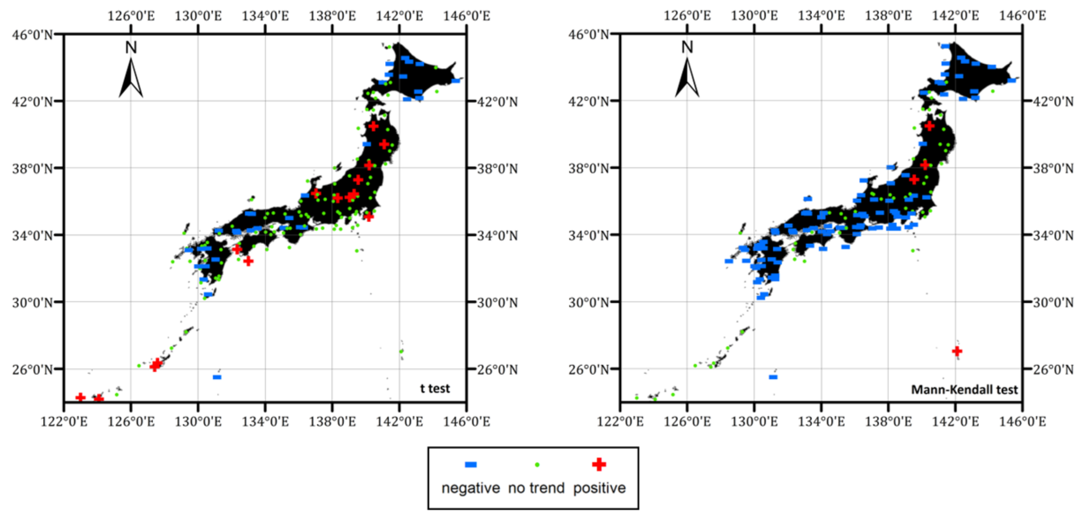
Another prior analysis on single-site observations is implemented directly for hourly precipitation data. Contrary to the monthly maximum precipitations, the hourly precipitations of many sites appear to have significant trends, thought the t-test and Mann Kendall tests give slightly different results. Figure 2 shows statistically significant positive and negative trends in hourly precipitations of single-site observations through Japan. The sites in high and low latitude regions have mainly negative trends, while the sites of middle latitude inner regions have positive trends.
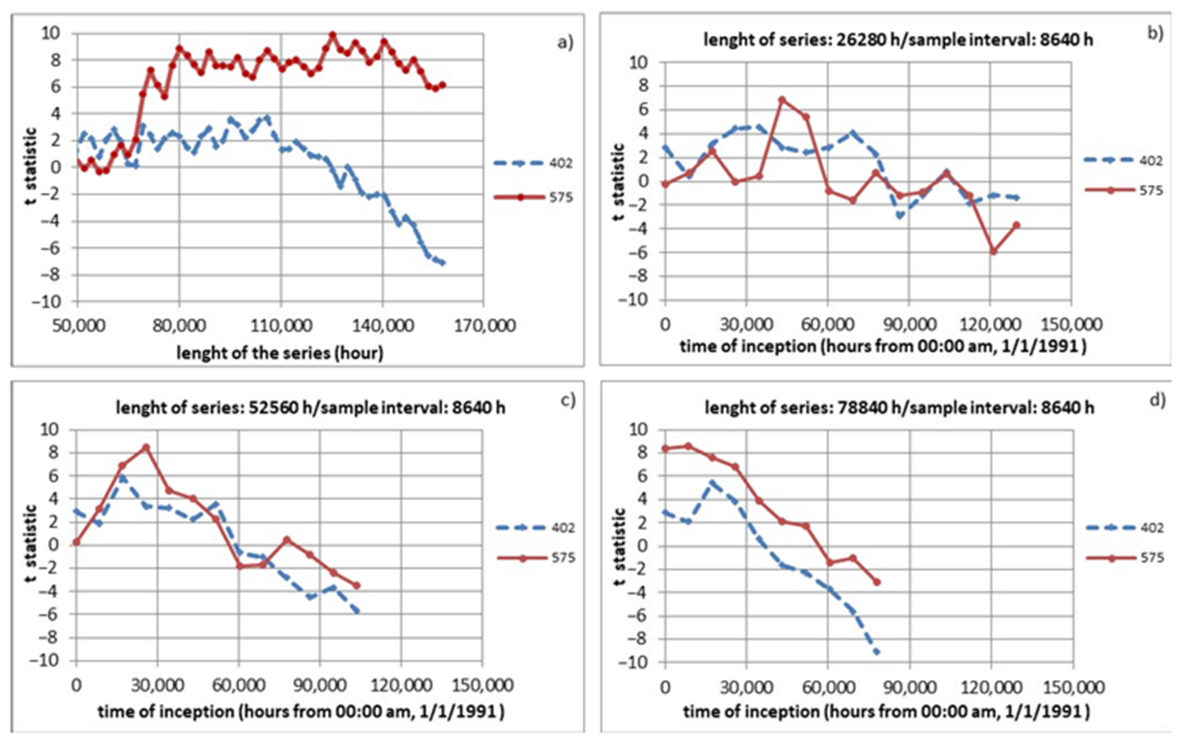
For the sites 402 and 575, which give respectively the highest negative and positive t scores, the considered lengths of hourly precipitation series are changed systematically (by 3 months) to see if t-scores change by the length of the series considered (Figure 3a). Moreover, in order to see the effect of different observation periods on t-scores, the time spans of the observations are changed systematically so as to have subseries on different time periods of whole length of the hourly series. For 26,280 h, 52,560 h and 78,840 h (i.e., 3, 6 and 9 years) series lengths, the subseries are so created that the time inceptions are systematically increased by 8640 h (approximately 1 year). Figure 3b–d shows the change of t-scores by these subseries of different observation periods, respectively for 26,280 h, 52,560 h and 78,840 h length series. This analysis indicated that the t-score therefore the acceptance of a trend hypothesis highly depends on the length of series. The lengthier series, more accurate the estimations on trend analyses. The considered periods of the observations are also vital to decide to the existence of a statistically significant trend, especially for small size series. For larger series, the difference between the t-statistic and critical t-values is getting larger, this helps us to clarify if there is a statistically significant trend.
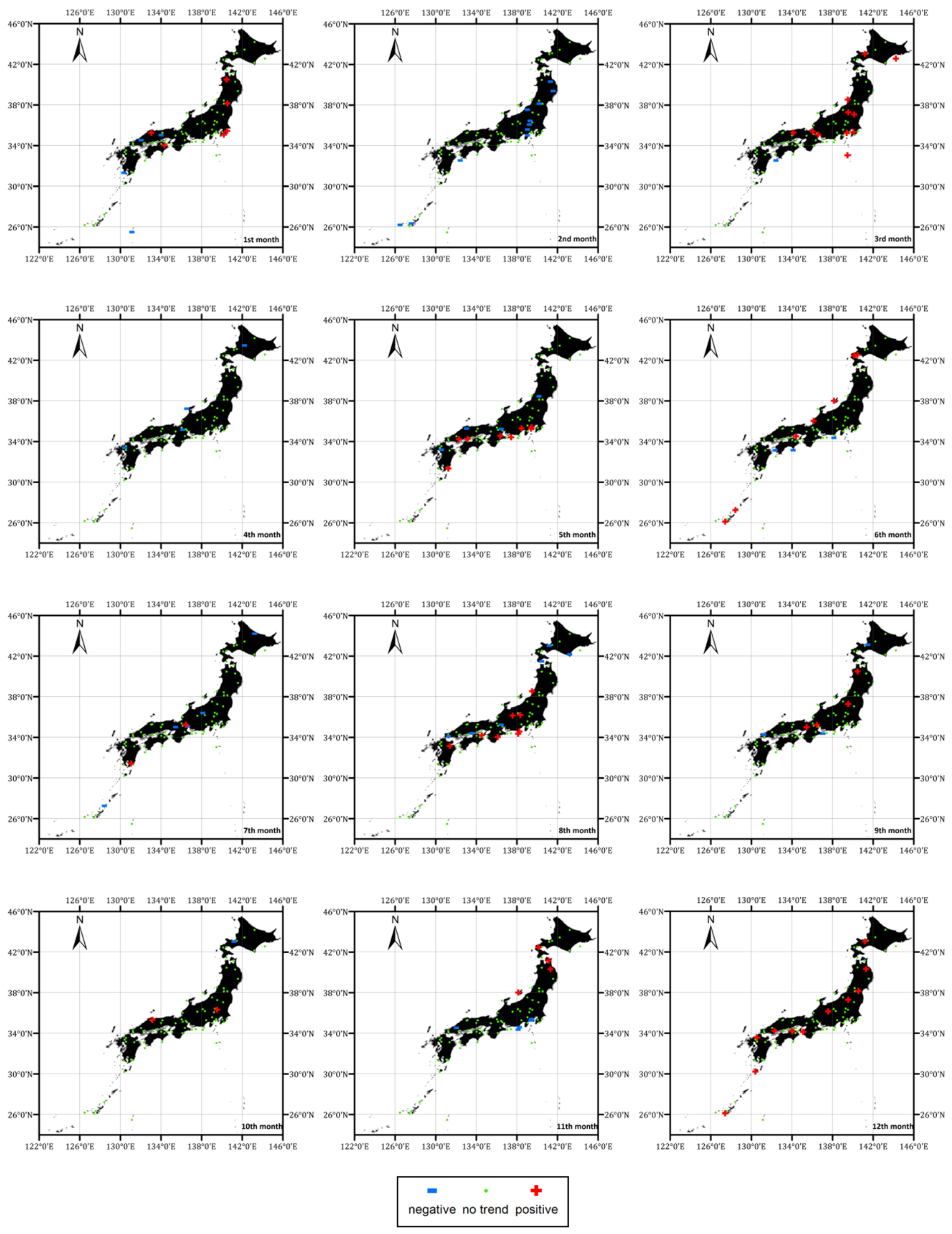
For single-site observations, the existence of trend is also investigated for monthly maximum precipitations of the same months of subsequent years, regarding that climatic extremes are more sensitive to climatic changes. The monthly maximum precipitation series are organized into 12 new time series, representing months. Both the t-test and Mann Kendall tests are used to test these data series for possible trends. The sites with significant trends are given in Figure 4. According to Figure 4, some sites have significant trends for some months, nonetheless no general pattern can be seen and proves a consistent trend supported by multi stations, geographically contiguous.
These prior analyses confirmed that trend analyses are highly sensitive to the length of series, observation period and the type of the test applied. The calculated trends lack geographical consistency and generally consider only a single statistic (e.g., maximum, mean etc.) of heavy precipitation. These facts demand regional studies that focus on climatic extremes, and further investigations of hourly data [3,41]. The need for further investigation on multi-station trend analysis has created the main motivation for this study. Aiming to develop a regional approach for investigation of a regional trend on heavy precipitations, this study introduces “the index precipitation method”, which defines a hydrologic homogeneous region with an identical frequency distribution of multi-site observations in order to verify the existence of a regional trend on heavy precipitations via various precipitation indices.
The index precipitation method needs a preliminary effort to refine discordant gauging sites. Two methods are applied to decide on discordant stations. The first one is Wilk’s test in Equation (5), for which the sites with are identified as discordant. The second one is Euclidean Distances between L-moment ratios of observations and theoretical distributions. This method considers the sites with comparably high distances as outlier sites. For a specific month, the breaking point on a graph of the sites vs. relevant distances (in increasing order) give the critical distance for the outliers. Calculated discordant (outlier) sites are given in Table 2.
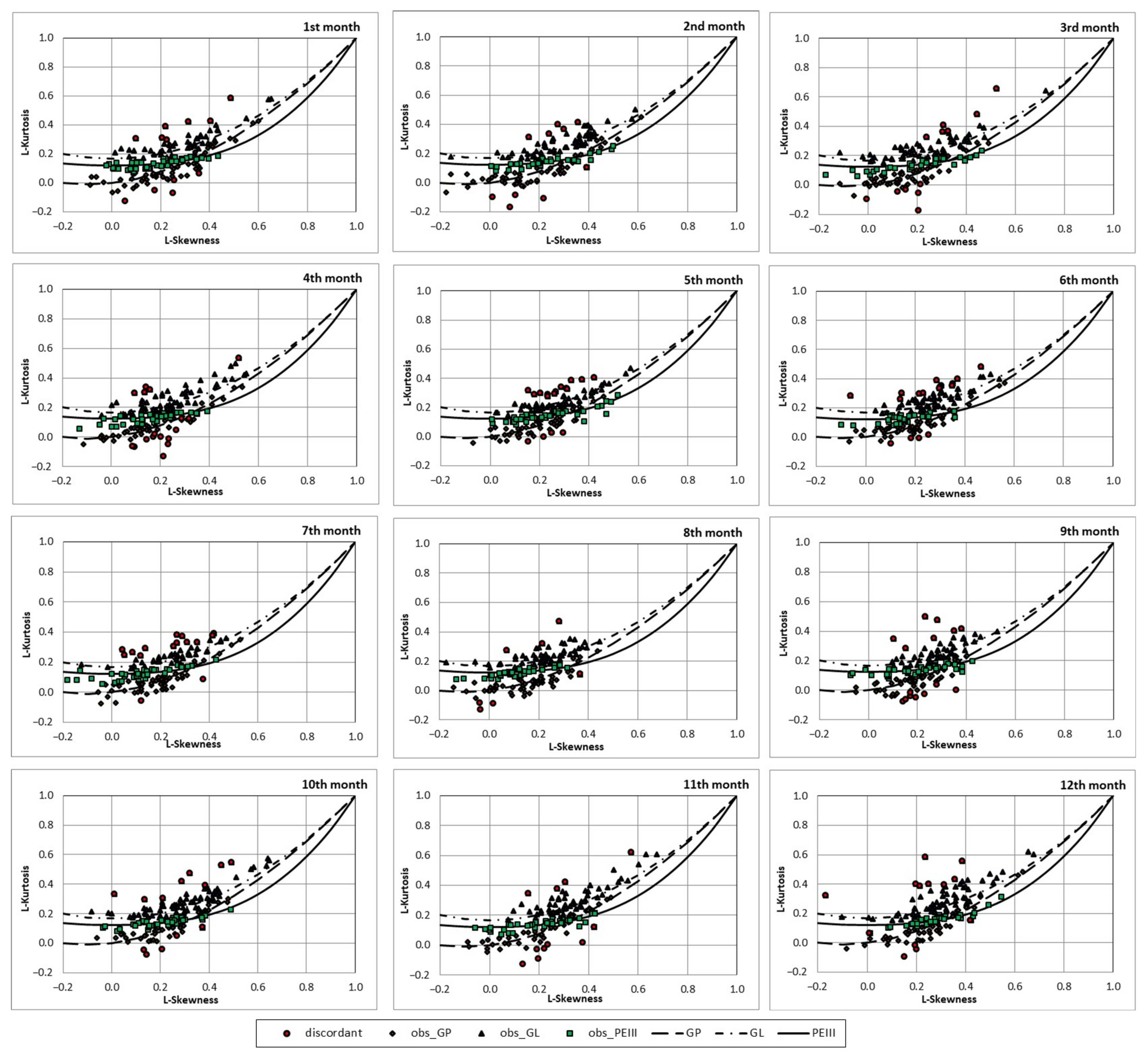
The index precipitation method requires a three-step verification for delineation of a homogeneous region. As a first step, in order to define the siteswith identical frequency distributions of maximum hourly precipitations, L-moment ratios of the site observations and theoretical distributions were calculated. Based on the L-moment ratio diagram, distances between the L-moment ratios of the observations and theoretical distributions were calculated. The frequency distributions best fitting to hourly precipitations were then investigated by means of the measure in Equation (9). The L-moment ratios—L skewness/L kurtosis—of the 150 sites and the L-moment ratios of Generalized Parteo (GP), Generalized Logistic (GL) and Pearson Type 3 (PEIII) distributions are plotted in Figure 5. Both the discordant sites and the sites with identical frequency distributions are shown in the Figure 5.
The second step of the index precipitation method requires to determine the sites with identical regional parameters, for the same frequency distribution sites. Hierarchical Clustering was applied to further classify the sites with an identical frequency distribution into the sites with similar frequency distribution parameters. Euclidean Distances between the frequency parameters , , were used to define the similarities for each month via Equation (10).
The significant numbers of hierarchical levels were decided based on the graphs of Euclidean distances vs. hierarchical steps, by finding the step after which the graph begins to level off. The obtained homogenous classes through which , , are statistically identical are given in Table 3. Where, n is the number of the sites in homogenous classes.
The third step of the index precipitation method was implemented by delineating homogenous classes into geographically contiguous homogeneous regions. Thiessen polygon method was used for this purpose. Each of the calculated homogenous regions therefore provided the assumptions of (1) identical frequency distribution, (2) identical frequency distribution parameters, (3) geographically continuity. The homogenous regions are shown in Figure 6.
The regional parameters obtained for the homogenous regions are given in Table 4.
Defining hydrologic characteristics of heavy precipitations, the 12 indices given in Equation (11) were used to verify the existence and consistency of the regional trends on the homogenous regions. For each homogenous region, the estimates of 12 indices were organized in time series of same months. Regional trends were tested for the homogenous regions by the t-test and Mann Kendall tests. The t and z values are given in Table 5.
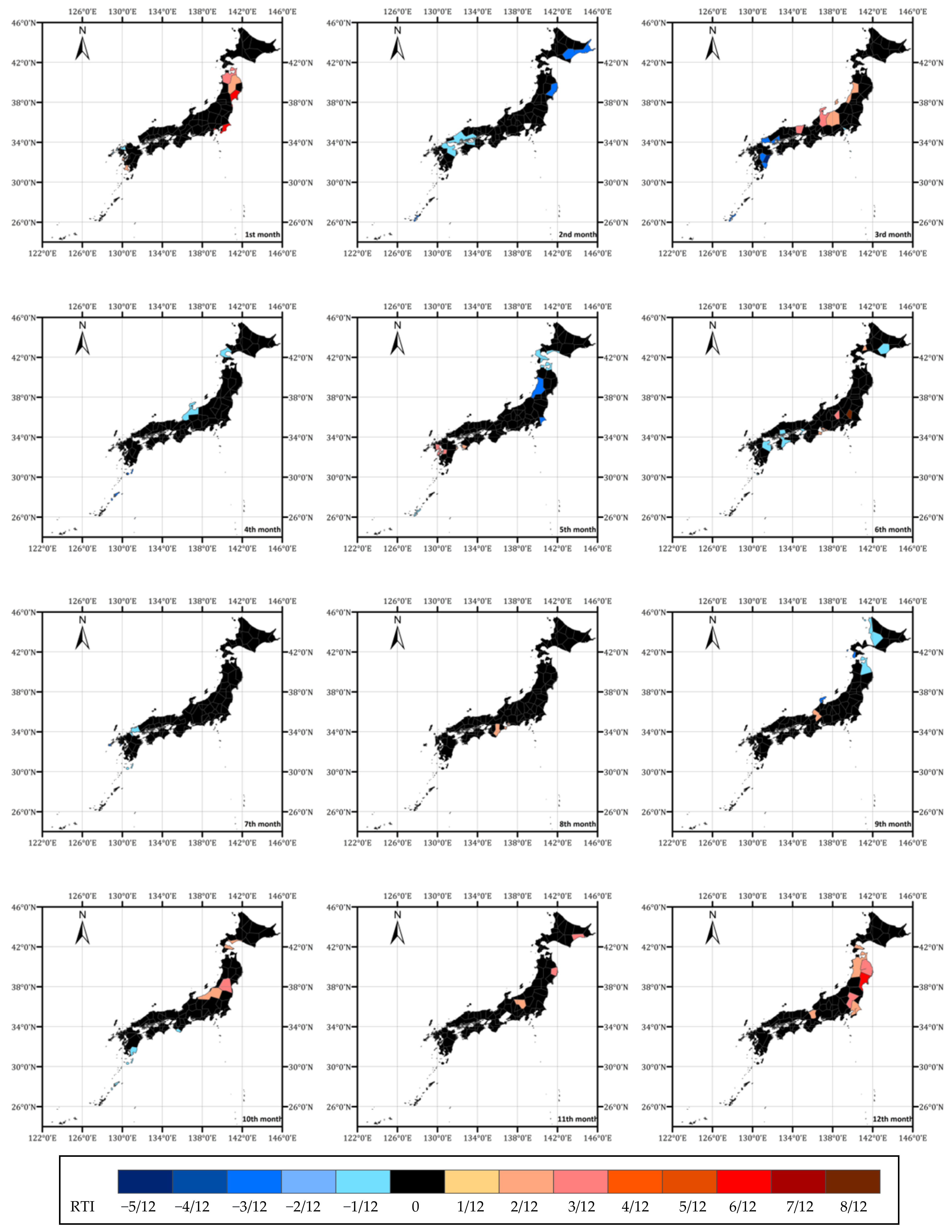
Figure 7 shows homogenous regions with significant trends, regarding the regional trend index.
The gauging sites in these homogenous regions with significant trends are listed in Table 6. The general picture of the regional analyses implemented along Japan has shown that temporal changes on heavy precipitations depend largely on season and geographical location. Statistically significant positive and negative trends have been detected, in changing intensities. Upper, middle and lower latitudes of the country; Pacific Ocean and Asia main continent sides of the country; hot, cold and rainy seasons may be considered to characterize these regional trends.
5. Conclusions
The Index Precipitation Method introduced herein provided a spatial consistency in the estimation of the temporal changes on heavy precipitations. Since homogenous regions are based on a statistically identical frequency distribution and parameters, the observed trends preserve statistical properties of precipitation frequencies on a considered study area. Homogenous regions and observed trends are less sensitive to sampling variation. Use of L-moment estimates in the delineation processes facilitated homogeneity analyses, while preserving high order statistical moments. Homogenous regions are geographically continuous and enclose geographically contiguous sites. In this respect, GIS provided an effective environment for the delineation processes and for the determination of homogenous regions.
Relying on the 12 indices that characterize heavy precipitations, the regional trend analyses made possible to take both the regional and temporal sampling variations into account. These indices define not solely the changes on the mean or extreme statistics of single-site observations, but also the regional changes on heavy precipitation. As a regional figure of merit and a trend severity measure, the regional trend index is a good indicator of the existence of a regionally verified consistent trend. Trend analyses along japan show that temporal changes of heavy precipitations depend highly on geographical location. Upper, middle and lower latitudes have similar trend behaviour. The regional trends change monthly. Rainy and cold periods indicate more evident trends.
It is concluded in the study that the Index Precipitation Method usefully defines homogenous regions for which the frequency behaviors of multisite precipitation observations are preserved. It is valuable especially for removing negative effects of sampling variations, missing data, regionally unsupported trend tests, use of statistical moment-based parameters, on single-site trend analyses. The Index Precipitation Method would be also advantageous for various hydrologic studies that need regional homogeneity and spatial verification/support for temporal changes. It is expected to reduce ambiguities in hydrologic modelling related to single-site temporal processes.
Funding
This research received no external funding.
Institutional Review Board Statement
Not applicable.
Informed Consent Statement
Not applicable.
Data Availability Statement
Not applicable.
Acknowledgments
I would like to thank to the Japan Society of Promotion of Science (JSPS) and Taikan Oki for their supports during the preparation of the manuscript. I also wish to acknowledge Kader Benli for her kind help on scripting.
Conflicts of Interest
The author declares no conflict of interest.
References
- Easterling, D.R.; Meehl, G.A.; Parmesan, C.; Changnon, S.A.; Karl, T.R.; Mearns, L.O. Climate extremes: Observations, modeling and impacts. Science 2000, 289, 2068–2074. [Google Scholar] [CrossRef] [PubMed] [Green Version]
- Karl, T.R.; Knight, R.W.; Plummer, N. Trends in hight-frequency climate variability in the twentieth century. Nature 1995, 377, 217–220. [Google Scholar] [CrossRef]
- Fujibe, F.; Yamazaki, N. Long term changes of heavy precipitation and dry weather in Japan. J. Meteorol. Soc. Jpn. 2006, 84, 1033–1046. [Google Scholar] [CrossRef] [Green Version]
- Partal, T.; Kahya, E. Trend analysis in Turkish precipitation data. Hydrol. Process. 2006, 20, 2011–2026. [Google Scholar] [CrossRef]
- Serrano, A.; Mateos, V.L.; Garcia, J.A. Trend analysis of monthly precipitation over the Iberian Peninsula for the period 1921–1995. Phys. Chem. Earth B 1999, 24, 85–90. [Google Scholar] [CrossRef]
- Piccarreta, M.; Capolongo, D.; Boenzi, F. Trend analysis of precipitation and drought in Basilicata, from 1923 to 2000 within a southern Italy context. Int. J. Climatol. 2004, 24, 907–922. [Google Scholar] [CrossRef]
- Stafford, J.M.; Wendler, G.; Curti, J. Temperature and precipitation of Alaska: 50-year trend analysis. Theor. Appl. Climatol. 2000, 67, 33–44. [Google Scholar] [CrossRef]
- Feidas, H.; Noulopoulou, C.H.; Makrogiannis, T.; Bora-Senta, E. Trend analysis of precipitation time series in Greece and their relationship with circulation using surface and satellite data: 1955–2001. Theor. Appl. Climatol. 2007, 87, 155–177. [Google Scholar] [CrossRef]
- Gemmer, M.; Becker, S.; Jiang, T. Observed monthly precipitation trends in China 1951–2002. Theor. Appl. Climatol. 2004, 77, 39–45. [Google Scholar] [CrossRef]
- Mekis, E.; Hogg, W.D. Rehabilitation and analysis of Canadian daily precipitation time series. Atmos. Ocean 1999, 37, 53–85. [Google Scholar] [CrossRef]
- Kunkel, K.E.; Andsager, K.; Easterling, D.R. Long-term trends in extreme precipitation events over the conterminous United States and Canada. J. Clim. 1999, 12, 2515–2527. [Google Scholar] [CrossRef] [Green Version]
- Chen, M.; Xie, P.; Janowiak, J.E.; Arkin, P.A. Global land precipitation: A 50-yr monthly analysis based on gauge observations. J. Hydrometeorol. 2002, 3, 249–266. [Google Scholar] [CrossRef]
- IPCC; Houghton, J.T.; Ding, Y.; Griggs, D.J.; Noguer, M.; Van der Linden, P.J.; Dai, X.; Maskell, K.; Johnson, C.A. (Eds.) Climate Change 2001: The Scientific Basis Contribution of Working Group I to the Third Assessment Report of the Intergovernmental Panel on Climate Change; Cambridge University Press: Cambridge, UK, 2001; p. 881. [Google Scholar]
- Bordi, I.; Fraedrich, K.; Suteara, A. Observed drought and wetness trends in Europe: An update. Hydrol. Earth Syst. Sci. 2009, 13, 1519–1530. [Google Scholar] [CrossRef] [Green Version]
- Katz, R.W.; Brown, B.G. Extreme events in a changing climate: Variability is more important than averages. Clim. Change 1992, 21, 289–302. [Google Scholar] [CrossRef]
- Semmler, T.; Jacob, D. Modeling extreme precipitation events: A climate change simulation for Europe. Glob. Planet. Change 2004, 44, 119–127. [Google Scholar] [CrossRef]
- Machiwal, D.; Kumar, S.; Meena, H.M.; Santra, P.; Singh, R.K.; Singh, D.V. Clustering of rainfall stations and distinguishing influential factors using PCA and HCA techniques over the western dry region of India. Meteorol. Appl. 2019, 26, 300–311. [Google Scholar] [CrossRef] [Green Version]
- Kirby, W.H.; Moss, M.E. Summary of flood-frequency analysis in the United States. J. Hydrol. 1987, 96, 5–14. [Google Scholar] [CrossRef]
- Mishra, B.K.; Takara, K.; Yamashiki, Y.; Tachikawa, Y. An assesment of predictive accuracy for two regional flood-frequency estimation methods, annual. J. Hydraul. Eng. JSCE 2010, 54, 7–12. [Google Scholar]
- Stedinger, J.R.; Tasker, G.D. Regional hydrologic analysis, 1: Ordinary weighted and generalized least squares compared. Water Resour. Res. 1985, 21, 1421. [Google Scholar] [CrossRef]
- Wallis, J.R.; Wood, E.F. Relative accuracy of log Pearson Type III procedures. J. Hydraul. Eng. ASCE 1985, 111, 1043–1056. [Google Scholar] [CrossRef]
- Burn, D.H. Evaluation of regional flood frequency analysis with a region of influence approach. Water Resour. Res. 1990, 26, 2257–2265. [Google Scholar] [CrossRef]
- Hosking, J.R.M.; Wallis, J.R. Regional Frequency Analysis; Cambridge University Press: Cambridge, UK, 1997; p. 224. [Google Scholar]
- Stedinger, J.R.; Lu, L.H. Appraisal of regional and index flood quantile estimators. Stoch. Hydrol. Hydraul. 1995, 9, 49–75. [Google Scholar] [CrossRef]
- Cunnane, C. Methods and merits of regional flood frequency analysis. J. Hydrol. 1988, 100, 269–290. [Google Scholar] [CrossRef]
- Japan Meteorological Agency (JMA). 2005. Available online: https://www.jma.go.jp/en/g3/ (accessed on 21 June 2019).
- Kajiwara, M.; Oki, T.; Matsumoto, J. Secular change in the frequency of heavy precipitation over Japan for 100 years. In Proceedings of the 2003 Spring Meeting of MJS, Washington, DC, USA, 12–13 April 2003. [Google Scholar]
- Takahashi, H. Secular variation in the occurrence property of summertime daily rainfall amount in and around the Tokyo metropolitan area. Tenki 2003, 50, 31–41. [Google Scholar]
- Van Gelder, P.; Mai, C.V. Distribution functions of extreme sea waves and river discharges. J. Hydraul. Res. 2008, 46, 280–291. [Google Scholar] [CrossRef]
- Dalrymple, T. Flood Frequency Analysis, Manual of Hydrology; Water Supply Paper Series No. 1543; U.S. Geological Survey: Washington, DC, USA, 1960; Chapter A.
- Sveinsson, O.G.B.; Salas, J.D.; Boes, D.C. Regional frequency analysis of extreme precipitation in northeastern Colorado and Fort Collins flood of 1997. J. Hydrol. Eng. 2002, 7, 1–49. [Google Scholar] [CrossRef]
- Norbiato, D.; Borga, M.; Sangati, M.; Zanon, F. Regional frequency analysis of extreme precipitation in the eastern Italian Alps and the August 29, 2003 flash flood. J. Hydrol. 2007, 345, 149–166. [Google Scholar] [CrossRef]
- Guttman, N.B. The use of L-moments in the determination of regional precipitation climates. J. Clim. 1993, 6, 2309–2325. [Google Scholar] [CrossRef] [Green Version]
- Hosking, J.R.M. L-moments: Analysis and estimation of distributions using liner combinations of order statistics. J. R. Statist. Soc. B 1990, 52, 105–124. [Google Scholar] [CrossRef]
- Parida, B.P.; Kachroo, R.K.; Shrestha, D.B. Regional flood frequency analysis of Mahi-Sabarmati basin using index flood pressure with L-moments. Water Resour. Manag. 1998, 12, 1–12. [Google Scholar] [CrossRef]
- Greenwood, J.A.; Landwehr, J.M.; Matalas, N.C.; Wallis, J.R. Probability weighted moments; Definition and relation to parameters of several distributions expressible in inverse form. Water Resour. Res. 1979, 15, 1049–1054. [Google Scholar] [CrossRef] [Green Version]
- Caroni, C.; Prescott, P. Sequential application of Wilks’s multivariate outliers test. Appl. Stat. 1992, 41, 355–364. [Google Scholar] [CrossRef]
- Vogel, R.M.; Fennessey, N.M. L-moment diagrams should reply product moment diagrams. Water Resour. Res. 1993, 29, 1745–1752. [Google Scholar] [CrossRef]
- Folland, C.K.; Frich, P.; Rayner, N.; Basnerr, T.; Parker, D.E.; Horton, B. Uncertainties in climate data set, A challenge for WHO. WMO Bull. 2000, 49, 59–68. [Google Scholar]
- Frich, P.; Alexander, L.V.; Marta, P.D.; Gleason, B.; Haylock, M.; Tank, A.M.G.K.; Peterson, T. Observed coherent changes in climatic extremes during the second half of the twentieth century. Clim. Res. 2002, 19, 193–212. [Google Scholar] [CrossRef] [Green Version]
- Folland, C.K.; Karl, T.R.; Salinger, M.J. Observed climate variability and change. Weather 2002, 57, 269–278. [Google Scholar] [CrossRef]
- Fujibe, F.; Yamazaki, N.; Katsuyama, M.; Kobayashi, K. The increasing trend of intense precipitation in Japan based on four-hourly data for a hundred years. SOLA 2005, 1, 41–44. [Google Scholar] [CrossRef] [Green Version]
- Onoz, B.; Bayazıt, M. The power of statistical tests trend for detection. Turk. J. Eng. Environ. Sci. 2003, 27, 247–251. [Google Scholar]
- Haan, C.T. Statistical Methods in Hydrology; The Iowa State University Press: Ames, IA, USA, 1977. [Google Scholar]
Figure 1.
The locations of 150 rainfall gauges having consistent records throughout the period of 1991–2010 for the study area.
Figure 1.
The locations of 150 rainfall gauges having consistent records throughout the period of 1991–2010 for the study area.

Figure 2.
Trends in hourly precipitations for 1991–2010 (trends approved by both the t-test and Mann-Kendall test for 0.95 confidence level).
Figure 2.
Trends in hourly precipitations for 1991–2010 (trends approved by both the t-test and Mann-Kendall test for 0.95 confidence level).

Figure 3.
Sampling behaviors of the t-statistic for hourly precipitations with different length of series. (a) shows the change of the t-scores by the length of series. (b–d) shows the effect of the different observation periods on the t-scores, corresponding to the different time spans of the observations, shifted systematically by 8640 h, for 26,280 h, 52,560 h and 78,840 h length series, respectively.

Figure 4.
Trends in monthly maximum precipitations for the same months along 1991–2010 (Trends approved by both the t-test and Mann Kendall test for 0.95 confidence level).
Figure 4.
Trends in monthly maximum precipitations for the same months along 1991–2010 (Trends approved by both the t-test and Mann Kendall test for 0.95 confidence level).

Figure 5.
L-moment ratio diagrams (Graphs show fitness of the L-moment ratios of the 150 sites and different theoretical distributions such as Generalized Parteo GP, Generalized Logistic GL and Pearson Type 3 PEIII distributions).
Figure 5.
L-moment ratio diagrams (Graphs show fitness of the L-moment ratios of the 150 sites and different theoretical distributions such as Generalized Parteo GP, Generalized Logistic GL and Pearson Type 3 PEIII distributions).

Figure 6.
Homogenous regions (They are defined in three steps; the first step is determination of the sites with identical frequency distributions such as Generalized Parteo (GP), Generalized Logistic (GL) and Pearson Type 3 (PEIII) distributions; the second step is determination of the sites with similar frequency parameters such as , , , among the sites with an identical frequency distribution; the last step is delineation of these sites with an identical distribution and similarly equal frequency parameters into geographically contiguous regions).

Figure 7.
The regional trend indices for homogenous regions (The regional trend index RTI indicates the percentage of trend indices with significant trend, for a homogenous region and month).
Figure 7.
The regional trend indices for homogenous regions (The regional trend index RTI indicates the percentage of trend indices with significant trend, for a homogenous region and month).


Table 1.
Resultant statistics of the trend analyses of the maximum hourly precipitations on the observation sites for 1991–2010 (the t-test and Mann-Kendall test are used to test the existences of significant trends for 0.95 confidence level).
Table 1.
Resultant statistics of the trend analyses of the maximum hourly precipitations on the observation sites for 1991–2010 (the t-test and Mann-Kendall test are used to test the existences of significant trends for 0.95 confidence level).
| Trends in Sites | ||||||
|---|---|---|---|---|---|---|
| Sites | 575 | 585 | 616 | 622 | 836 | 940 |
| b (mm/month) | 0.011 | 0.023 | 0.020 | 0.020 | 0.040 | 0.035 |
| t values | * | 2.266 | 2.090 | 2.370 | 1.961 | 2.464 |
| z values | 1.989 | 2.093 | 1.537 | * | * | 1.963 |
* there is no statistically significant trend for this site, based on the test used; b: regression coefficient; t: t statistics (see Equation (14)); z: z statistic (see Equation (16)).
Table 2.
Discordancy Analyses for the period of 1991–2010 (The discordant stations are the sites for which Discordancy Measure Di of Wilks’s test are or for which Euclidean Distances dmin between the L-moment ratios of the observations and theoretical distributions are—considerably high compared to the rest of the data set—larger than the critical distance for that month).
| 1th Month | 2th Month | 3th Month | 4th Month | ||||||||||||
| Station | dmin | Station | D | Station | dmin | Station | D | Station | dmin | Station | D | Station | dmin | Station | D |
| 622 | 0.167 | 784 | 5.525 | 666 | 0.182 | 413 | 7.802 | 401 | 0.184 | 401 | 9.586 | 612 | 0.149 | 684 | 4.342 |
| 784 | 0.166 | 512 | 4.671 | 653 | 0.171 | 636 | 6.138 | 640 | 0.143 | 740 | 7.453 | 769 | 0.127 | 675 | 4.272 |
| 672 | 0.154 | 585 | 4.425 | 742 | 0.150 | 776 | 5.695 | 656 | 0.119 | 430 | 6.164 | 670 | 0.123 | 651 | 4.216 |
| 817 | 0.153 | 898 | 4.293 | 424 | 0.118 | 587 | 4.872 | 942 | 0.118 | 626 | 5.252 | 622 | 0.116 | 605 | 3.635 |
| 780 | 0.134 | 762 | 4.212 | 819 | 0.116 | 653 | 4.190 | 750 | 0.104 | 741 | 4.343 | 651 | 0.104 | 893 | 3.605 |
| 766 | 0.131 | 440 | 4.175 | 570 | 0.111 | 895 | 3.961 | 754 | 0.103 | 899 | 4.334 | 893 | 0.095 | 662 | 3.498 |
| 649 | 0.105 | 672 | 3.767 | 631 | 0.110 | 666 | 3.942 | 831 | 0.096 | 784 | 4.043 | 768 | 0.091 | ||
| 626 | 0.104 | 815 | 3.566 | 822 | 0.110 | 837 | 3.840 | 610 | 0.094 | 656 | 3.902 | 755 | 0.085 | ||
| 616 | 0.101 | 421 | 0.097 | 742 | 3.146 | 597 | 0.077 | 662 | 0.068 | ||||||
| 674 | 0.095 | 636 | 0.077 | 612 | 0.061 | 657 | 0.062 | ||||||||
| 618 | 0.082 | 585 | 0.060 | 767 | 0.060 | ||||||||||
| 654 | 0.077 | 592 | 0.052 | 830 | 0.055 | ||||||||||
| 421 | 0.053 | ||||||||||||||
| 606 | 0.052 | ||||||||||||||
| 618 | 0.040 | ||||||||||||||
| 674 | 0.039 | ||||||||||||||
| 570 | 0.037 | ||||||||||||||
| 5th Month | 6th Month | 7th Month | 8th Month | ||||||||||||
| Station | dmin | Station | D | Station | dmin | Station | D | Station | dmin | Station | D | Station | dmin | Station | D |
| 837 | 0.126 | 777 | 6.064 | 754 | 0.133 | 824 | 8.727 | 807 | 0.138 | 575 | 6.005 | 632 | 0.208 | 632 | 9.369 |
| 629 | 0.111 | 780 | 5.651 | 824 | 0.114 | 624 | 6.802 | 674 | 0.120 | 812 | 5.655 | 822 | 0.122 | 684 | 8.802 |
| 624 | 0.094 | 626 | 4.335 | 822 | 0.112 | 649 | 5.819 | 819 | 0.116 | 776 | 4.675 | 587 | 0.105 | 440 | 6.681 |
| 835 | 0.092 | 837 | 3.826 | 684 | 0.104 | 684 | 4.473 | 605 | 0.106 | 945 | 4.471 | 655 | 0.103 | 746 | 4.936 |
| 607 | 0.092 | 663 | 3.741 | 682 | 0.098 | 602 | 3.691 | 405 | 0.091 | 637 | 3.511 | 674 | 0.090 | 598 | 4.677 |
| 821 | 0.091 | 649 | 3.701 | 648 | 0.096 | 835 | 3.487 | 597 | 0.090 | 426 | 3.447 | 768 | 0.079 | 761 | 3.491 |
| 407 | 0.090 | 618 | 3.141 | 590 | 0.090 | 770 | 3.298 | 892 | 0.089 | 407 | 3.243 | 684 | 0.062 | 822 | 3.125 |
| 772 | 0.078 | 636 | 0.084 | 655 | 3.287 | 762 | 0.088 | 819 | 3.232 | 762 | 3.064 | ||||
| 756 | 0.076 | 778 | 0.083 | 893 | 0.079 | 807 | 3.051 | 411 | 3.047 | ||||||
| 893 | 0.076 | 428 | 0.082 | 581 | 0.077 | ||||||||||
| 570 | 0.074 | 823 | 0.081 | 616 | 0.074 | ||||||||||
| 777 | 0.073 | 805 | 0.080 | 668 | 0.063 | ||||||||||
| 411 | 0.073 | 831 | 0.080 | 595 | 0.062 | ||||||||||
| 672 | 0.071 | 423 | 0.076 | 404 | 0.054 | ||||||||||
| 512 | 0.070 | 654 | 0.070 | 656 | 0.053 | ||||||||||
| 831 | 0.070 | 581 | 0.070 | ||||||||||||
| 598 | 0.068 | 582 | 0.066 | ||||||||||||
| 648 | 0.063 | ||||||||||||||
| 663 | 0.060 | ||||||||||||||
| 940 | 0.058 | ||||||||||||||
| 636 | 0.040 | ||||||||||||||
| 9th Month | 10th Month | 11th Month | 12th Month | ||||||||||||
| Station | dmin | Station | D | Station | dmin | Station | D | Station | dmin | Station | D | Station | dmin | Station | D |
| 574 | 0.257 | 574 | 6.647 | 632 | 0.187 | 620 | 6.130 | 592 | 0.159 | 675 | 5.012 | 570 | 0.326 | 404 | 9.117 |
| 830 | 0.211 | 584 | 4.482 | 620 | 0.165 | 604 | 5.897 | 624 | 0.154 | 626 | 4.679 | 588 | 0.212 | 750 | 7.069 |
| 822 | 0.167 | 830 | 4.453 | 784 | 0.162 | 435 | 4.899 | 807 | 0.153 | 807 | 4.344 | 584 | 0.185 | 570 | 6.661 |
| 584 | 0.148 | 822 | 4.163 | 759 | 0.148 | 800 | 4.584 | 836 | 0.149 | 575 | 4.031 | 587 | 0.167 | 770 | 5.135 |
| 610 | 0.115 | 632 | 3.937 | 815 | 0.132 | 767 | 3.817 | 424 | 0.145 | 592 | 4.009 | 428 | 0.163 | 421 | 4.678 |
| 423 | 0.114 | 654 | 3.583 | 420 | 0.116 | 617 | 3.649 | 616 | 0.130 | 424 | 3.982 | 843 | 0.134 | 892 | 4.468 |
| 766 | 0.112 | 440 | 3.363 | 624 | 0.111 | 815 | 3.418 | 626 | 0.126 | 651 | 3.837 | 402 | 0.132 | 590 | 4.295 |
| 626 | 0.110 | 653 | 3.150 | 607 | 0.106 | 632 | 3.342 | 822 | 0.100 | 836 | 3.825 | 756 | 0.130 | 585 | 4.172 |
| 817 | 0.105 | 598 | 0.094 | 612 | 3.293 | 823 | 0.088 | 588 | 3.208 | 404 | 0.128 | 581 | 4.048 | ||
| 426 | 0.105 | 433 | 0.085 | 759 | 3.277 | 769 | 0.080 | 838 | 0.109 | 741 | 3.914 | ||||
| 648 | 0.105 | 829 | 0.081 | 420 | 3.201 | 675 | 0.075 | 835 | 0.083 | 588 | 3.096 | ||||
| 512 | 0.093 | 604 | 0.068 | 898 | 0.056 | 417 | 3.049 | ||||||||
| 741 | 0.093 | 893 | 0.057 | 590 | 0.045 | ||||||||||
| 827 | 0.076 | ||||||||||||||
| 682 | 0.070 | ||||||||||||||
Table 3.
Statistics of the probabilistic distribution parameters in homogeneous classes (Calculated by Equations (6)–(8)).
Table 3.
Statistics of the probabilistic distribution parameters in homogeneous classes (Calculated by Equations (6)–(8)).
| Month | Class | Generalized Pareto | Generalized Logistic | Pearson Type III | ||||||||||||||||||
|---|---|---|---|---|---|---|---|---|---|---|---|---|---|---|---|---|---|---|---|---|---|---|
| n | Mean | Std Dev | n | Mean | Std Dev | n | Mean | Std Dev | ||||||||||||||
| α | k | β | α | k | β | α | k | β | α | k | β | α | k | β | α | k | β | |||||
| 1 | 1 | 12 | 0 | 1.565 | 2.565 | 0 | 0.242 | 0.242 | 23 | 0.932 | −0.170 | 0.221 | 0.040 | 0.075 | 0.073 | 8 | 0.241 | 2.156 | 0.365 | 0.155 | 0.412 | 0.105 |
| 2 | 14 | 0 | 2.387 | 3.387 | 0 | 0.198 | 0.198 | 19 | 0.835 | −0.362 | 0.240 | 0.041 | 0.041 | 0.066 | 8 | 0.406 | 1.005 | 0.628 | 0.189 | 0.293 | 0.246 | |
| 3 | 11 | 0 | 0.939 | 1.939 | 0 | 0.122 | 0.122 | 3 | 0.595 | −0.615 | 0.233 | 0.081 | 0.056 | 0.045 | 3 | −0.324 | 10.861 | 0.122 | 0.347 | 0.338 | 0.030 | |
| 4 | 13 | 0 | 0.363 | 1.363 | 0 | 0.218 | 0.218 | 4 | 0.161 | 4.090 | 0.206 | 0.262 | 0.660 | 0.062 | ||||||||
| 5 | 2 | 0 | 5.412 | 6.412 | 0 | 0.055 | 0.055 | 2 | 0.122 | 8.054 | 0.109 | 0.103 | 0.484 | 0.006 | ||||||||
| 6 | 2 | 0.055 | 5.668 | 0.169 | 0.476 | 0.287 | 0.093 | |||||||||||||||
| 2 | 1 | 14 | 0 | 1.443 | 2.443 | 0 | 0.176 | 0.176 | 22 | 0.909 | −0.230 | 0.226 | 0.029 | 0.049 | 0.051 | 23 | 0.172 | 1.949 | 0.620 | 0.197 | 1.128 | 0.428 |
| 2 | 19 | 0 | 0.713 | 1.713 | 0 | 0.259 | 0.259 | 24 | 0.816 | −0.383 | 0.243 | 0.042 | 0.024 | 0.050 | 3 | −0.036 | 7.843 | 0.131 | 0.299 | 1.430 | 0.029 | |
| 3 | 7 | 0 | 2.182 | 3.182 | 0 | 0.221 | 0.221 | 3 | 0.976 | −0.124 | 0.116 | 0.008 | 0.031 | 0.021 | ||||||||
| 4 | 2 | 0 | 4.689 | 5.689 | 0 | 0.026 | 0.026 | 3 | 0.979 | −0.052 | 0.234 | 0.014 | 0.021 | 0.062 | ||||||||
| 5 | 4 | 0 | 2.830 | 3.830 | 0 | 0.104 | 0.104 | 2 | 0.812 | −0.526 | 0.150 | 0.028 | 0.069 | 0.014 | ||||||||
| 6 | 4 | 0 | 3.774 | 4.774 | 0 | 0.249 | 0.249 | |||||||||||||||
| 7 | 2 | 0 | 5.688 | 6.688 | 0 | 0.354 | 0.354 | |||||||||||||||
| 3 | 1 | 21 | 0 | 2.442 | 3.442 | 0 | 0.340 | 0.340 | 20 | 0.837 | −0.370 | 0.225 | 0.030 | 0.058 | 0.027 | 16 | 0.435 | 1.309 | 0.490 | 0.156 | 0.626 | 0.177 |
| 2 | 17 | 0 | 1.314 | 2.314 | 0 | 0.320 | 0.320 | 31 | 0.941 | −0.180 | 0.199 | 0.020 | 0.064 | 0.047 | 4 | 0.121 | 3.650 | 0.240 | 0.135 | 0.200 | 0.031 | |
| 3 | 11 | 0 | 3.849 | 4.849 | 0 | 0.469 | 0.469 | 7 | 1.003 | 0.009 | 0.171 | 0.015 | 0.049 | 0.027 | 2 | −0.759 | 26.178 | 0.067 | 0.639 | 0.412 | 0.023 | |
| 4 | 2 | −0.593 | 14.802 | 0.108 | 0.000 | 1.632 | 0.012 | |||||||||||||||
| 4 | 1 | 17 | 0 | 1.751 | 2.751 | 0 | 0.138 | 0.138 | 27 | 0.879 | −0.263 | 0.251 | 0.039 | 0.053 | 0.035 | 5 | −0.124 | 7.009 | 0.161 | 0.351 | 0.297 | 0.052 |
| 2 | 13 | 0 | 1.037 | 2.037 | 0 | 0.159 | 0.159 | 3 | 0.828 | −0.467 | 0.169 | 0.020 | 0.039 | 0.003 | 25 | 0.251 | 2.368 | 0.382 | 0.141 | 1.005 | 0.188 | |
| 3 | 5 | 0 | 2.130 | 3.130 | 0 | 0.066 | 0.066 | 16 | 0.961 | −0.099 | 0.232 | 0.022 | 0.049 | 0.033 | 2 | −0.798 | 14.358 | 0.127 | 0.541 | 0.845 | 0.045 | |
| 4 | 4 | 0 | 3.083 | 4.083 | 0 | 0.037 | 0.037 | 6 | 0.713 | −0.486 | 0.262 | 0.045 | 0.055 | 0.023 | ||||||||
| 5 | 2 | 0 | 0.633 | 1.633 | 0 | 0.097 | 0.097 | |||||||||||||||
| 6 | 2 | 0 | 2.713 | 3.713 | 0 | 0.098 | 0.098 | |||||||||||||||
| 5 | 1 | 7 | 0 | 2.863 | 3.863 | 0 | 0.031 | 0.031 | 6 | 0.911 | −0.290 | 0.168 | 0.011 | 0.018 | 0.010 | 10 | 0.290 | 1.755 | 0.412 | 0.162 | 0.404 | 0.081 |
| 2 | 6 | 0 | 2.473 | 3.473 | 0 | 0.076 | 0.076 | 22 | 0.898 | −0.234 | 0.246 | 0.025 | 0.040 | 0.034 | 5 | 0.307 | 2.831 | 0.245 | 0.102 | 0.230 | 0.029 | |
| 3 | 15 | 0 | 1.216 | 2.216 | 0 | 0.145 | 0.145 | 7 | 0.958 | −0.126 | 0.203 | 0.010 | 0.032 | 0.029 | 8 | 0.440 | 0.578 | 1.037 | 0.118 | 0.172 | 0.345 | |
| 4 | 10 | 0 | 1.823 | 2.823 | 0 | 0.205 | 0.205 | 13 | 0.820 | −0.414 | 0.214 | 0.025 | 0.039 | 0.030 | 4 | 0.215 | 3.724 | 0.212 | 0.079 | 0.199 | 0.029 | |
| 5 | 2 | 0.992 | −0.025 | 0.200 | 0.001 | 0.005 | 0.013 | 2 | −0.057 | 11.899 | 0.089 | 0.109 | 0.108 | 0.010 | ||||||||
| 6 | 2 | 0.818 | −0.323 | 0.301 | 0.014 | 0.008 | 0.014 | 2 | −0.147 | 9.931 | 0.115 | 0.116 | 0.124 | 0.010 | ||||||||
| 7 | 2 | 0.732 | −0.558 | 0.192 | 0.012 | 0.014 | 0.018 | 2 | 0.026 | 5.204 | 0.188 | 0.261 | 0.120 | 0.055 | ||||||||
| 8 | 2 | −0.124 | 6.974 | 0.162 | 0.275 | 0.361 | 0.048 | |||||||||||||||
| 6 | 1 | 16 | 0 | 1.576 | 2.576 | 0 | 0.125 | 0.125 | 17 | 0.908 | −0.205 | 0.258 | 0.019 | 0.033 | 0.028 | 7 | 0.269 | 1.596 | 0.496 | 0.112 | 0.526 | 0.145 |
| 2 | 5 | 0 | 1.996 | 2.996 | 0 | 0.061 | 0.061 | 19 | 0.843 | −0.323 | 0.258 | 0.032 | 0.039 | 0.030 | 6 | −0.269 | 6.235 | 0.206 | 0.138 | 0.760 | 0.030 | |
| 3 | 17 | 0 | 1.083 | 2.083 | 0 | 0.164 | 0.164 | 5 | 0.917 | −0.262 | 0.178 | 0.007 | 0.018 | 0.010 | 4 | −0.302 | 9.193 | 0.143 | 0.153 | 0.762 | 0.024 | |
| 4 | 6 | 0 | 2.918 | 3.918 | 0 | 0.112 | 0.112 | 5 | 0.971 | −0.080 | 0.229 | 0.009 | 0.035 | 0.044 | 7 | 0.173 | 3.678 | 0.224 | 0.209 | 0.651 | 0.044 | |
| 5 | 5 | 0 | 2.407 | 3.407 | 0 | 0.138 | 0.138 | 4 | 0.762 | −0.460 | 0.242 | 0.015 | 0.037 | 0.037 | 3 | −0.605 | 12.560 | 0.130 | 0.269 | 1.032 | 0.033 | |
| 6 | 2 | 0 | 3.331 | 4.331 | 0 | 0.044 | 0.044 | 2 | 0.846 | −0.501 | 0.133 | 0.030 | 0.053 | 0.001 | ||||||||
| 7 | 2 | 0 | 0.687 | 1.687 | 0 | 0.053 | 0.053 | |||||||||||||||
| 7 | 1 | 19 | 0 | 1.644 | 2.644 | 0 | 0.157 | 0.157 | 15 | 0.931 | −0.155 | 0.264 | 0.024 | 0.054 | 0.039 | 15 | 0.188 | 2.114 | 0.442 | 0.296 | 1.053 | 0.184 |
| 2 | 10 | 0 | 0.615 | 1.615 | 0 | 0.128 | 0.128 | 15 | 0.854 | −0.288 | 0.282 | 0.020 | 0.031 | 0.043 | 5 | −0.722 | 9.731 | 0.178 | 0.132 | 0.794 | 0.024 | |
| 3 | 15 | 0 | 1.107 | 2.107 | 0 | 0.147 | 0.147 | 4 | 0.748 | −0.427 | 0.283 | 0.039 | 0.037 | 0.027 | 9 | −0.107 | 5.722 | 0.194 | 0.206 | 0.562 | 0.038 | |
| 4 | 4 | 0 | 2.130 | 3.130 | 0 | 0.053 | 0.053 | 3 | 0.868 | −0.395 | 0.165 | 0.024 | 0.051 | 0.001 | 2 | −0.337 | 14.275 | 0.093 | 0.391 | 0.694 | 0.023 | |
| 5 | 2 | 0 | 3.410 | 4.410 | 0 | 0.097 | 0.097 | |||||||||||||||
| 6 | 3 | 0 | 2.736 | 3.736 | 0 | 0.207 | 0.207 | |||||||||||||||
| 8 | 1 | 18 | 0 | 1.794 | 2.794 | 0 | 0.170 | 0.170 | 15 | 0.829 | −0.325 | 0.278 | 0.039 | 0.033 | 0.042 | 18 | 0.015 | 3.390 | 0.381 | 0.180 | 2.027 | 0.178 |
| 2 | 10 | 0 | 1.267 | 2.267 | 0 | 0.089 | 0.089 | 25 | 0.897 | −0.215 | 0.278 | 0.021 | 0.026 | 0.048 | 7 | −0.912 | 13.642 | 0.142 | 0.442 | 2.953 | 0.028 | |
| 3 | 10 | 0 | 0.837 | 1.837 | 0 | 0.130 | 0.130 | 8 | 0.943 | −0.121 | 0.280 | 0.013 | 0.017 | 0.034 | 2 | −2.109 | 51.334 | 0.061 | 1.151 | 1.310 | 0.024 | |
| 4 | 7 | 0 | 0.391 | 1.391 | 0 | 0.079 | 0.079 | 5 | 0.998 | −0.006 | 0.255 | 0.016 | 0.041 | 0.049 | ||||||||
| 5 | 5 | 0 | 2.373 | 3.373 | 0 | 0.165 | 0.165 | |||||||||||||||
| 9 | 1 | 16 | 0 | 1.366 | 2.366 | 0 | 0.074 | 0.074 | 33 | 0.855 | −0.299 | 0.265 | 0.028 | 0.049 | 0.032 | 13 | 0.349 | 1.132 | 0.620 | 0.117 | 0.334 | 0.214 |
| 2 | 2 | 0 | 2.618 | 3.618 | 0 | 0.001 | 0.001 | 4 | 0.772 | −0.462 | 0.226 | 0.040 | 0.044 | 0.010 | 7 | −0.101 | 4.600 | 0.239 | 0.199 | 0.335 | 0.039 | |
| 3 | 12 | 0 | 1.707 | 2.707 | 0 | 0.124 | 0.124 | 8 | 0.939 | −0.144 | 0.257 | 0.014 | 0.041 | 0.041 | 4 | −0.861 | 16.101 | 0.116 | 0.154 | 0.378 | 0.008 | |
| 4 | 5 | 0 | 0.522 | 1.522 | 0 | 0.132 | 0.132 | 6 | 0.194 | 2.355 | 0.346 | 0.147 | 0.461 | 0.049 | ||||||||
| 5 | 8 | 0 | 1.003 | 2.003 | 0 | 0.103 | 0.103 | |||||||||||||||
| 6 | 5 | 0 | 2.192 | 3.192 | 0 | 0.116 | 0.116 | |||||||||||||||
| 7 | 4 | 0 | 3.049 | 4.049 | 0 | 0.072 | 0.072 | |||||||||||||||
| 10 | 1 | 18 | 0 | 1.180 | 2.180 | 0 | 0.258 | 0.258 | 24 | 0.862 | −0.261 | 0.297 | 0.020 | 0.041 | 0.031 | 11 | 0.243 | 1.597 | 0.480 | 0.146 | 0.258 | 0.095 |
| 2 | 13 | 0 | 0.430 | 1.430 | 0 | 0.214 | 0.214 | 20 | 0.782 | −0.395 | 0.274 | 0.039 | 0.034 | 0.032 | 5 | −0.160 | 4.913 | 0.237 | 0.088 | 0.304 | 0.027 | |
| 3 | 5 | 0 | 2.197 | 3.197 | 0 | 0.302 | 0.302 | 3 | 1.009 | 0.033 | 0.208 | 0.011 | 0.045 | 0.046 | 3 | −0.110 | 3.442 | 0.324 | 0.039 | 0.363 | 0.027 | |
| 4 | 12 | 0.943 | −0.125 | 0.270 | 0.015 | 0.029 | 0.035 | 4 | 0.310 | 0.706 | 1.039 | 0.114 | 0.174 | 0.354 | ||||||||
| 5 | 4 | 0.628 | −0.628 | 0.206 | 0.047 | 0.029 | 0.048 | 2 | −0.001 | 2.376 | 0.431 | 0.122 | 0.374 | 0.119 | ||||||||
| 6 | 2 | 0.710 | −0.543 | 0.218 | 0.024 | 0.043 | 0.016 | |||||||||||||||
| 11 | 1 | 6 | 0 | 1.915 | 2.915 | 0 | 0.137 | 0.137 | 23 | 0.864 | −0.268 | 0.282 | 0.024 | 0.036 | 0.029 | 19 | 0.272 | 1.311 | 0.673 | 0.158 | 0.533 | 0.333 |
| 2 | 16 | 0 | 1.129 | 2.129 | 0 | 0.172 | 0.172 | 12 | 0.802 | −0.380 | 0.265 | 0.036 | 0.022 | 0.048 | 5 | 0.170 | 3.797 | 0.223 | 0.253 | 0.628 | 0.084 | |
| 3 | 13 | 0 | 0.528 | 1.528 | 0 | 0.198 | 0.198 | 5 | 0.695 | −0.467 | 0.300 | 0.039 | 0.035 | 0.038 | ||||||||
| 4 | 6 | 0 | 3.146 | 4.146 | 0 | 0.255 | 0.255 | 5 | 0.932 | −0.255 | 0.152 | 0.019 | 0.067 | 0.029 | ||||||||
| 5 | 5 | 0 | 2.548 | 3.548 | 0 | 0.108 | 0.108 | 4 | 0.947 | −0.114 | 0.270 | 0.024 | 0.038 | 0.041 | ||||||||
| 6 | 4 | 0.776 | −0.549 | 0.163 | 0.048 | 0.042 | 0.027 | |||||||||||||||
| 7 | 2 | 0.613 | −0.654 | 0.194 | 0.073 | 0.030 | 0.060 | |||||||||||||||
| 12 | 1 | 22 | 0 | 0.249 | 1.249 | 0 | 0.186 | 0.186 | 34 | 0.804 | −0.345 | 0.302 | 0.051 | 0.058 | 0.073 | 15 | 0.243 | 1.326 | 0.598 | 0.243 | 0.368 | 0.222 |
| 2 | 5 | 0 | 4.017 | 5.017 | 0 | 0.189 | 0.189 | 14 | 0.931 | −0.203 | 0.208 | 0.016 | 0.051 | 0.064 | 7 | −0.097 | 2.766 | 0.400 | 0.212 | 0.358 | 0.080 | |
| 3 | 5 | 0 | 1.695 | 2.695 | 0 | 0.282 | 0.282 | 5 | 0.649 | −0.504 | 0.303 | 0.045 | 0.039 | 0.033 | 4 | 0.304 | 0.488 | 1.430 | 0.172 | 0.119 | 0.117 | |
| 4 | 8 | 0 | 0.893 | 1.893 | 0 | 0.209 | 0.209 | 5 | 0.993 | −0.033 | 0.154 | 0.022 | 0.093 | 0.025 | ||||||||
| 5 | 4 | 0 | 2.941 | 3.941 | 0 | 0.222 | 0.222 | 2 | 0.623 | −0.665 | 0.179 | 0.017 | 0.015 | 0.020 | ||||||||
| 6 | 2 | 0 | 4.689 | 5.689 | 0 | 0.157 | 0.157 | |||||||||||||||
Table 4.
Homogenous regions and regional parameters (Throughout a homogenous region with n sites, the regional frequency distribution and parameters , , are statistically identical).
Table 4.
Homogenous regions and regional parameters (Throughout a homogenous region with n sites, the regional frequency distribution and parameters , , are statistically identical).
| Month | Class | Generalized Pareto | Generalized Logistic | Pearson Type III | |||||||||||||||||||
|---|---|---|---|---|---|---|---|---|---|---|---|---|---|---|---|---|---|---|---|---|---|---|---|
| n | Mean | Std Dev | n | Mean | Std Dev | n | Mean | Std Dev | |||||||||||||||
| α | k | β | α | k | β | α | k | β | α | k | β | α | k | β | α | k | β | ||||||
| 1 | 1 | 7 | 0 | 2.399 | 3.399 | 0 | 0.195 | 0.195 | 3 | 0.964 | −0.173 | 0.123 | 0.018 | 0.090 | 0.017 | 3 | 0.222 | 2.346 | 0.336 | 0.069 | 0.446 | 0.040 | |
| 2 | 3 | 0 | 1.032 | 2.032 | 0 | 0.026 | 0.026 | 5 | 0.956 | −0.128 | 0.192 | 0.034 | 0.083 | 0.083 | |||||||||
| 3 | 3 | 0 | 0.280 | 1.280 | 0 | 0.136 | 0.136 | 4 | 0.894 | −0.240 | 0.250 | 0.032 | 0.010 | 0.068 | |||||||||
| 4 | 3 | 0 | 0.401 | 1.401 | 0 | 0.206 | 0.206 | 3 | 0.816 | −0.363 | 0.263 | 0.018 | 0.040 | 0.028 | |||||||||
| 5 | 4 | 0 | 0.295 | 1.295 | 0 | 0.321 | 0.321 | 3 | 0.869 | −0.342 | 0.203 | 0.024 | 0.019 | 0.042 | |||||||||
| 2 | 1 | 3 | 0 | 1.320 | 2.320 | 0 | 0.132 | 0.132 | 7 | 0.918 | −0.211 | 0.221 | 0.028 | 0.053 | 0.032 | 5 | 0.146 | 2.639 | 0.395 | 0.203 | 1.054 | 0.246 | |
| 2 | 3 | 0 | 0.786 | 1.786 | 0 | 0.284 | 0.284 | 4 | 0.805 | −0.387 | 0.254 | 0.031 | 0.035 | 0.025 | 5 | 0.112 | 1.585 | 0.685 | 0.181 | 0.840 | 0.306 | ||
| 3 | 6 | 0 | 0.637 | 1.637 | 0 | 0.296 | 0.296 | ||||||||||||||||
| 3 | 1 | 4 | 0 | 2.302 | 3.302 | 0 | 0.203 | 0.203 | 3 | 0.806 | −0.424 | 0.221 | 0.020 | 0.045 | 0.016 | 3 | 0.384 | 1.301 | 0.614 | 0.091 | 0.729 | 0.379 | |
| 2 | 5 | 0 | 2.508 | 3.508 | 0 | 0.398 | 0.398 | 3 | 0.827 | −0.371 | 0.237 | 0.026 | 0.029 | 0.013 | |||||||||
| 3 | 5 | 0 | 1.214 | 2.214 | 0 | 0.134 | 0.134 | 3 | 0.940 | −0.141 | 0.253 | 0.032 | 0.079 | 0.029 | |||||||||
| 4 | 4 | 0 | 4.115 | 5.115 | 0 | 0.301 | 0.301 | 6 | 0.946 | −0.194 | 0.164 | 0.020 | 0.079 | 0.027 | |||||||||
| 5 | 6 | 0.933 | −0.196 | 0.198 | 0.021 | 0.049 | 0.048 | ||||||||||||||||
| 6 | 5 | 0.946 | −0.154 | 0.212 | 0.014 | 0.055 | 0.033 | ||||||||||||||||
| 4 | 1 | 5 | 0 | 1.701 | 2.701 | 0 | 0.190 | 0.190 | 15 | 0.871 | −0.274 | 0.256 | 0.037 | 0.047 | 0.042 | 4 | 0.205 | 1.703 | 0.519 | 0.205 | 0.792 | 0.154 | |
| 2 | 3 | 0 | 1.808 | 2.808 | 0 | 0.064 | 0.064 | 3 | 0.828 | −0.467 | 0.169 | 0.020 | 0.039 | 0.003 | 7 | 0.306 | 1.831 | 0.500 | 0.090 | 1.243 | 0.251 | ||
| 3 | 5 | 0 | 1.033 | 2.033 | 0 | 0.168 | 0.168 | 4 | 0.956 | −0.091 | 0.258 | 0.040 | 0.077 | 0.049 | |||||||||
| 4 | 3 | 0.956 | −0.109 | 0.238 | 0.017 | 0.028 | 0.037 | ||||||||||||||||
| 5 | 1 | 4 | 0 | 1.254 | 2.254 | 0 | 0.197 | 0.197 | 3 | 0.914 | −0.287 | 0.164 | 0.015 | 0.027 | 0.010 | ||||||||
| 2 | 3 | 0 | 1.212 | 2.212 | 0 | 0.082 | 0.082 | 3 | 0.965 | −0.100 | 0.211 | 0.010 | 0.028 | 0.009 | |||||||||
| 3 | 3 | 0.835 | −0.402 | 0.204 | 0.021 | 0.017 | 0.028 | ||||||||||||||||
| 6 | 1 | 3 | 0.084 | 0.802 | 1.834 | 0.146 | 0.872 | 0.817 | 4 | 1.564 | 1.447 | 0.149 | 1.646 | 1.964 | 0.101 | ||||||||
| 2 | 3 | 0.086 | 0.527 | 1.575 | 0.105 | 0.760 | 1.272 | 3 | 1.252 | 0.223 | 0.178 | 0.493 | 0.518 | 0.156 | |||||||||
| 3 | 3 | 0.916 | −0.184 | 0.249 | 0.063 | 0.129 | 0.018 | ||||||||||||||||
| 7 | 1 | 8 | 0 | 1.682 | 2.682 | 0 | 0.149 | 0.149 | 4 | 0.151 | 2.318 | 0.406 | 0.339 | 1.275 | 0.138 | ||||||||
| 2 | 3 | 0 | 1.170 | 2.170 | 0 | 0.097 | 0.097 | 3 | 0.289 | 1.308 | 0.653 | 0.140 | 0.793 | 0.284 | |||||||||
| 8 | 1 | 4 | 0 | 1.912 | 2.912 | 0 | 0.032 | 0.032 | 4 | 0.830 | −0.341 | 0.263 | 0.021 | 0.011 | 0.036 | 3 | −0.039 | 3.589 | 0.409 | 0.236 | 2.192 | 0.293 | |
| 2 | 3 | 0.898 | −0.200 | 0.297 | 0.017 | 0.025 | 0.032 | 3 | 0.080 | 3.055 | 0.413 | 0.231 | 2.580 | 0.223 | |||||||||
| 3 | 3 | 0.885 | −0.234 | 0.280 | 0.015 | 0.016 | 0.037 | ||||||||||||||||
| 9 | 1 | 5 | 0 | 1.382 | 2.382 | 0 | 0.080 | 0.080 | 4 | 0.848 | −0.305 | 0.272 | 0.016 | 0.038 | 0.030 | ||||||||
| 2 | 14 | 0.848 | −0.312 | 0.263 | 0.030 | 0.044 | 0.037 | ||||||||||||||||
| 3 | 3 | 0.835 | −0.345 | 0.249 | 0.029 | 0.044 | 0.004 | ||||||||||||||||
| 10 | 1 | 4 | 0 | 0.973 | 1.973 | 0 | 0.166 | 0.166 | 6 | 0.865 | −0.254 | 0.298 | 0.025 | 0.044 | 0.028 | ||||||||
| 2 | 3 | 0 | 1.582 | 2.582 | 0 | 0.146 | 0.146 | 4 | 0.853 | −0.280 | 0.290 | 0.008 | 0.012 | 0.019 | |||||||||
| 3 | 5 | 0 | 0.452 | 1.452 | 0 | 0.167 | 0.167 | 3 | 0.870 | −0.268 | 0.271 | 0.030 | 0.060 | 0.027 | |||||||||
| 4 | 4 | 0.862 | −0.241 | 0.327 | 0.021 | 0.051 | 0.035 | ||||||||||||||||
| 5 | 4 | 0.797 | −0.405 | 0.247 | 0.043 | 0.019 | 0.044 | ||||||||||||||||
| 6 | 3 | 0.947 | −0.114 | 0.273 | 0.017 | 0.026 | 0.022 | ||||||||||||||||
| 11 | 1 | 3 | 0 | 0.486 | 1.486 | 0 | 0.190 | 0.190 | 6 | 0.861 | −0.262 | 0.295 | 0.029 | 0.042 | 0.029 | 5 | 0.186 | 1.020 | 0.848 | 0.081 | 0.290 | 0.231 | |
| 2 | 7 | 0.866 | −0.262 | 0.286 | 0.023 | 0.033 | 0.036 | ||||||||||||||||
| 12 | 1 | 3 | 0 | 0.301 | 1.301 | 0 | 0.214 | 0.214 | 11 | 0.802 | −0.340 | 0.302 | 0.053 | 0.052 | 0.050 | 4 | 0.172 | 1.148 | 0.806 | 0.082 | 0.518 | 0.252 | |
| 2 | 8 | 0 | 0.315 | 1.315 | 0 | 0.142 | 0.142 | 6 | 0.835 | −0.290 | 0.314 | 0.014 | 0.023 | 0.021 | |||||||||
| 3 | 4 | 0.770 | −0.357 | 0.332 | 0.054 | 0.064 | 0.023 | ||||||||||||||||
| 4 | 4 | 0.761 | −0.314 | 0.413 | 0.013 | 0.034 | 0.035 | ||||||||||||||||
| 5 | 3 | 0.921 | −0.153 | 0.305 | 0.023 | 0.032 | 0.039 | ||||||||||||||||
| 6 | 4 | 0.929 | −0.228 | 0.182 | 0.007 | 0.045 | 0.032 | ||||||||||||||||
Table 5.
The t and z statistics for different indices (Bold values show statistically significant trends in the relevant indices for the considered homogenous regions and month. The regional trend index RTI indicates the percentage of the indices with significant trends, for a homogenous region and month).
| Months | Polygon | I1 | I2 | I3 | I4 | I5 | I6 | I7 | I8 | I9 | I10 | I11 | I12 | Regional Trend Index | ||||||||||||
|---|---|---|---|---|---|---|---|---|---|---|---|---|---|---|---|---|---|---|---|---|---|---|---|---|---|---|
| t | z | t | z | t | z | t | z | t | z | t | z | t | z | t | z | t | z | t | z | t | z | t | z | |||
| 1 | 41 | −0.357 | −0.455 | −0.604 | −0.455 | −0.607 | −0.190 | −0.523 | −0.342 | −0.127 | 0.000 | −0.732 | −0.720 | −2.446 | −1.756 | −2.446 | −1.756 | −2.383 | −1.682 | −2.383 | −1.682 | 0.702 | 0.608 | 1.024 | 0.954 | −0.333 |
| 33 | −0.918 | −0.833 | −1.111 | −1.023 | −1.768 | −1.988 | −1.949 | −1.823 | −0.673 | −0.455 | −0.771 | −0.341 | −0.903 | −0.708 | −1.182 | −0.829 | −0.829 | −0.765 | −1.003 | −0.765 | 0.513 | 1.142 | 0.325 | 1.067 | −0.083 | |
| 12 | 0.057 | 0.076 | −0.086 | 0.038 | −1.857 | −0.726 | −1.258 | −0.303 | 0.036 | 0.038 | −0.227 | 0.342 | −1.473 | −0.861 | −0.991 | −0.418 | −1.487 | −0.773 | −1.190 | −0.773 | 1.104 | 1.742 | 0.875 | 2.055 | 0.083 | |
| 45 | −0.437 | 0.000 | −0.593 | 0.114 | −1.434 | −0.190 | −1.821 | −0.912 | 0.844 | 1.136 | 0.889 | 1.327 | −1.684 | −1.000 | −1.181 | −0.796 | −1.840 | −1.102 | −1.588 | −0.997 | 1.869 | 2.064 | 1.713 | 1.982 | 0.167 | |
| 67 | 1.045 | 0.872 | 1.048 | 0.530 | 1.668 | 1.602 | 1.535 | 1.258 | 0.314 | 0.493 | 0.582 | 0.720 | 1.922 | 1.769 | 1.922 | 1.769 | 1.884 | 1.707 | 1.884 | 1.707 | 1.696 | 2.048 | 1.832 | 2.167 | 0.167 | |
| 52 | 1.743 | 1.894 | 2.068 | 1.970 | 2.003 | 1.155 | 1.902 | 1.240 | 0.997 | 0.833 | 1.544 | 1.061 | 1.472 | 1.121 | 1.328 | 1.121 | 1.497 | 1.121 | 1.384 | 1.121 | 2.785 | 2.771 | 2.773 | 2.929 | 0.333 | |
| 29 | 0.756 | 1.061 | 1.089 | 0.985 | 2.768 | 2.352 | 2.622 | 2.312 | −0.983 | 0.000 | −0.753 | 0.265 | 2.383 | 2.131 | 2.443 | 2.138 | 2.440 | 2.126 | 2.371 | 2.223 | 0.231 | 0.379 | 0.457 | 0.152 | 0.500 | |
| 2 | 80 | 0.497 | 0.000 | 0.852 | 0.152 | −0.593 | −0.381 | −0.823 | −1.027 | 1.204 | 1.212 | 1.743 | 1.709 | −1.530 | −2.102 | −1.530 | −2.037 | −1.530 | −1.962 | −1.530 | −1.962 | 0.483 | −0.266 | 0.511 | 0.000 | −0.333 |
| 85 | −0.557 | −0.455 | −1.322 | −0.682 | −0.950 | −1.645 | −0.383 | −0.684 | −0.032 | −0.227 | −0.458 | −0.379 | −1.287 | −1.962 | −1.287 | −1.822 | −1.287 | −1.962 | −1.287 | −1.962 | 0.557 | −0.190 | −0.376 | −0.950 | −0.250 | |
| 12 | −0.935 | −0.909 | −1.001 | −0.833 | −2.158 | −1.818 | −2.139 | −1.970 | −0.922 | −0.152 | −0.864 | 0.000 | −0.807 | −1.121 | −1.150 | −1.121 | −0.945 | −1.121 | −1.388 | −1.121 | 0.525 | 0.645 | 0.594 | 0.836 | −0.167 | |
| 43 | 0.641 | −0.379 | 0.557 | −0.227 | 0.986 | 0.343 | 0.959 | 0.038 | 0.399 | −0.303 | −1.229 | −1.972 | 1.134 | 0.462 | 1.358 | 0.548 | 1.185 | 0.544 | 1.455 | 0.670 | 0.656 | 0.341 | 0.217 | −0.228 | −0.083 | |
| 82 | 0.304 | 0.341 | 0.302 | 0.606 | 0.756 | −0.343 | 0.769 | −0.190 | 1.681 | 1.554 | 2.031 | 1.439 | 0.834 | 0.771 | 0.834 | 0.771 | 0.834 | 0.771 | 0.834 | 0.771 | 0.185 | −0.494 | 0.697 | −0.153 | 0.083 | |
| 3 | 14 | −2.443 | −2.085 | −2.458 | −2.121 | −1.992 | −1.593 | −2.536 | −1.937 | −2.321 | −1.742 | −2.452 | −1.972 | −0.748 | −0.781 | −0.748 | −0.781 | −0.660 | −0.773 | −0.660 | −0.773 | 0.047 | −0.607 | −0.427 | −0.959 | −0.500 |
| 12 | −0.763 | −0.758 | −0.719 | −0.682 | −0.936 | −1.061 | −0.740 | −0.909 | −2.089 | −1.894 | −2.777 | −2.088 | −1.795 | −2.071 | −1.795 | −2.071 | −1.603 | −1.731 | −1.603 | −1.731 | −1.445 | −1.296 | −1.442 | −1.449 | −0.333 | |
| 1 | −2.024 | −2.500 | −1.868 | −2.121 | −0.602 | −1.140 | −1.148 | −1.253 | −2.107 | −2.204 | −1.753 | −1.554 | −0.423 | −0.879 | −0.423 | −0.879 | −0.445 | −0.870 | −0.445 | −0.870 | −1.341 | −1.070 | −0.805 | −0.535 | −0.250 | |
| 22 | −0.833 | −0.948 | −0.519 | −0.455 | −0.152 | −0.228 | −0.314 | −0.229 | −1.165 | −0.720 | −1.056 | −0.759 | −2.259 | −1.096 | −1.953 | −1.009 | −2.355 | −1.091 | −2.115 | −1.091 | −1.064 | −1.366 | −0.056 | −0.800 | −0.250 | |
| 28 | −1.097 | −0.379 | −0.560 | 0.000 | 0.924 | 0.873 | 0.380 | 1.138 | −2.076 | −2.045 | −2.124 | −1.972 | 0.915 | 1.356 | 1.448 | 1.458 | 0.844 | 1.353 | 1.361 | 1.450 | −0.132 | −0.266 | −0.121 | −0.343 | −0.167 | |
| 33 | −1.298 | −1.175 | −1.093 | −0.606 | 1.623 | 1.480 | 2.547 | 2.428 | −2.445 | −2.312 | −2.457 | −1.669 | 1.476 | 1.376 | 1.221 | 1.376 | 1.695 | 1.454 | 1.599 | 1.363 | −1.327 | −1.596 | −0.893 | −1.485 | −0.083 | |
| 5 | 0.018 | −0.303 | 0.444 | −0.076 | 1.260 | 1.062 | 1.427 | 1.101 | −0.453 | −0.872 | 0.832 | 0.000 | 1.603 | 1.944 | 1.432 | 1.654 | 1.486 | 2.049 | 1.543 | 1.882 | 0.388 | −0.569 | 0.826 | −0.383 | 0.083 | |
| 15 | 0.564 | 0.530 | 0.885 | 0.455 | 0.623 | 0.228 | 0.707 | 0.114 | −1.005 | −0.456 | −1.251 | −1.023 | 0.630 | 0.000 | 0.596 | 0.000 | 0.682 | 0.097 | 0.599 | 0.000 | 2.284 | 1.026 | 1.289 | 0.195 | 0.083 | |
| 50 | −0.264 | −0.379 | −0.097 | −0.341 | 1.856 | 1.833 | 1.123 | 1.329 | −0.673 | −0.606 | 0.136 | 0.530 | 1.187 | 1.691 | 2.125 | 2.103 | 1.325 | 1.674 | 2.113 | 1.717 | −0.114 | −0.910 | 0.498 | −0.153 | 0.167 | |
| 27 | 1.169 | 0.758 | 1.946 | 1.515 | 2.004 | 1.889 | 2.003 | 2.128 | 0.588 | 0.303 | 0.913 | 0.303 | 0.862 | 1.202 | 0.227 | 0.789 | 1.329 | 2.007 | 0.794 | 1.893 | 1.088 | 0.341 | 0.420 | 0.000 | 0.250 | |
| 4 | 10 | −2.012 | −1.894 | −2.018 | −1.667 | −1.839 | −1.061 | −0.653 | −0.948 | −2.178 | −1.515 | −1.816 | −1.214 | −0.963 | −1.372 | −1.432 | −1.567 | −1.062 | −1.380 | −1.663 | −1.463 | −1.542 | −0.418 | −1.230 | −0.769 | −0.250 |
| 50 | −0.233 | −0.379 | −0.043 | −0.190 | −2.088 | −2.015 | −1.199 | −0.991 | −0.521 | −0.379 | −0.312 | 0.000 | 0.227 | 0.372 | 0.227 | 0.372 | −0.611 | 0.157 | −0.611 | 0.157 | 0.123 | −0.038 | 0.129 | −0.114 | −0.083 | |
| 69 | −0.439 | −0.455 | −0.373 | 0.000 | −1.275 | −1.719 | −1.243 | −1.979 | −0.197 | −0.152 | −0.149 | −0.341 | 0.000 | 0.118 | 0.000 | 0.118 | −0.042 | 0.059 | −0.055 | 0.000 | 0.165 | 0.152 | 0.229 | 0.304 | −0.083 | |
| 5 | 38 | −0.487 | 0.152 | −0.384 | −0.379 | −2.027 | −1.290 | −1.596 | −0.645 | 0.918 | 1.138 | 1.587 | 1.556 | −1.961 | −1.297 | −1.633 | −1.185 | −2.000 | −1.354 | −1.849 | −1.354 | −1.374 | −0.533 | −0.560 | −0.153 | −0.250 |
| 27 | −1.454 | −1.515 | −1.076 | −1.591 | 0.510 | 1.714 | −0.787 | 0.797 | −1.622 | −1.364 | −1.637 | −1.251 | 0.253 | 1.160 | 1.311 | 1.327 | 0.093 | 1.102 | 0.900 | 1.156 | −2.717 | −1.671 | −2.659 | −1.982 | −0.167 | |
| 10 | −1.084 | 0.038 | −1.176 | 0.000 | −0.712 | −0.229 | −0.924 | −0.190 | −0.442 | 0.493 | −0.478 | 0.342 | −0.808 | −0.590 | −0.784 | −0.590 | −0.806 | −0.530 | −0.776 | −0.647 | −2.453 | −1.138 | −1.704 | −0.879 | −0.083 | |
| 30 | −1.162 | −0.530 | −1.302 | −0.455 | −0.807 | −0.190 | −1.118 | −0.303 | −0.417 | 0.190 | −0.571 | 0.000 | −0.227 | 0.000 | −0.227 | 0.000 | −0.419 | −0.262 | −0.419 | −0.262 | −1.928 | −1.101 | −1.972 | −1.609 | −0.083 | |
| 49 | −0.490 | 0.152 | −1.103 | −0.227 | −2.125 | −1.371 | −1.707 | −0.569 | 0.200 | 0.758 | −0.299 | 0.152 | −1.004 | −0.735 | −0.873 | −0.735 | −0.956 | −0.682 | −0.843 | −0.787 | −0.396 | 0.000 | 0.680 | 0.191 | −0.083 | |
| 15 | 1.071 | 1.742 | 0.663 | 1.439 | 0.560 | 1.366 | 0.717 | 1.327 | 2.166 | 1.894 | 1.875 | 1.897 | 0.494 | 0.586 | 0.494 | 0.586 | 0.292 | 0.483 | 0.292 | 0.483 | 1.502 | 1.441 | 1.314 | 1.446 | 0.083 | |
| 19 | 2.077 | 0.872 | 1.771 | 1.061 | −1.664 | −0.493 | −1.070 | −0.227 | 1.973 | 1.136 | 1.946 | 1.175 | −1.003 | −0.875 | −1.003 | −0.875 | −1.164 | −0.870 | −1.164 | −0.870 | 0.961 | 0.267 | 0.882 | 0.114 | 0.167 | |
| 12 | 2.009 | 0.909 | 1.153 | 0.833 | −0.575 | −0.721 | 0.157 | 0.076 | 1.357 | 0.531 | 1.139 | 0.455 | −0.817 | −0.740 | −1.503 | −0.983 | −0.940 | −0.727 | −1.560 | −1.000 | 3.292 | 2.244 | 2.971 | 1.646 | 0.250 | |
| 6 | 81 | −1.147 | −1.591 | −1.079 | −1.439 | −0.481 | −0.797 | −0.438 | −0.228 | −0.967 | −1.212 | −0.725 | −0.833 | 0.502 | 0.633 | 0.643 | 0.789 | 0.572 | 0.682 | 0.644 | 0.682 | −2.393 | −2.352 | −2.647 | −2.436 | −0.167 |
| 2 | −0.362 | −0.493 | −0.389 | −0.985 | 0.693 | −0.266 | 0.884 | −0.038 | −0.692 | −0.909 | −0.342 | −0.796 | 0.903 | 0.089 | 0.610 | 0.000 | 1.052 | 0.000 | 0.854 | 0.000 | −1.686 | −0.949 | −2.443 | −1.485 | −0.083 | |
| 10 | −1.176 | −0.455 | −1.065 | −0.227 | 0.242 | 0.190 | 0.149 | 0.265 | −1.309 | −0.227 | −1.075 | −0.228 | 0.169 | 0.422 | 0.456 | 0.584 | 0.198 | 0.367 | 0.438 | 0.472 | −2.107 | −1.253 | −1.415 | −0.570 | −0.083 | |
| 12 | −0.667 | −1.212 | −0.691 | −1.212 | 0.845 | 0.076 | 0.491 | −0.152 | −1.342 | −1.818 | −1.400 | −1.970 | 0.349 | 0.000 | 0.349 | 0.000 | 0.548 | 0.091 | 0.548 | 0.091 | −1.246 | −1.329 | −1.094 | −1.520 | −0.083 | |
| 16 | −1.338 | −1.439 | −1.345 | −1.591 | −0.388 | −0.531 | −0.621 | −0.835 | −1.825 | −1.742 | −2.331 | −2.165 | 0.285 | 0.315 | 0.000 | 0.211 | 0.249 | 0.367 | 0.002 | 0.262 | 0.278 | 0.000 | −0.119 | 0.000 | −0.083 | |
| 19 | −1.360 | −1.061 | −1.222 | −1.591 | −0.787 | −0.948 | −1.127 | −1.212 | −0.915 | −1.253 | −0.958 | −1.402 | −0.499 | −0.389 | −0.499 | −0.389 | −0.333 | −0.387 | −0.333 | −0.387 | −2.150 | −1.444 | −1.608 | −0.921 | −0.083 | |
| 27 | −0.434 | −0.909 | −0.214 | −0.872 | 0.381 | 0.000 | 0.671 | −0.076 | −1.514 | −1.970 | −1.304 | −1.517 | −0.759 | −0.492 | −0.759 | −0.492 | −0.750 | −0.420 | −0.750 | −0.420 | 0.265 | 0.645 | 0.212 | 0.538 | −0.083 | |
| 44 | 1.142 | 1.175 | 1.004 | 0.417 | 3.378 | 2.161 | 3.469 | 1.972 | 0.308 | 0.683 | 0.104 | 0.455 | 1.431 | 0.292 | 1.311 | 0.394 | 1.590 | 0.435 | 1.543 | 0.676 | −0.352 | −0.038 | −0.494 | −0.270 | 0.167 | |
| 49 | −0.818 | −0.227 | −1.094 | −0.493 | 2.119 | 1.604 | 1.443 | 1.979 | −1.176 | −0.455 | −1.298 | −0.569 | 0.000 | 0.000 | 0.000 | 0.000 | 0.000 | 0.000 | 0.000 | 0.000 | −1.127 | −0.265 | −1.013 | −0.305 | 0.167 | |
| 78 | −0.709 | −1.136 | −0.215 | −0.114 | 2.823 | 1.821 | 2.603 | 1.782 | −1.391 | −1.288 | −1.143 | −0.985 | 1.718 | 1.132 | 1.840 | 1.132 | 1.962 | 1.547 | 2.122 | 1.547 | 0.383 | 0.461 | 0.174 | 0.308 | 0.333 | |
| 30 | 1.825 | 2.121 | 1.796 | 2.273 | 3.039 | 3.222 | 2.331 | 2.500 | 1.553 | 1.591 | 1.585 | 1.327 | 2.021 | 2.214 | 2.010 | 2.154 | 2.299 | 2.504 | 2.288 | 2.388 | 1.204 | 1.554 | 1.267 | 1.556 | 0.667 | |
| 7 | 40 | −0.169 | −0.379 | −0.272 | −0.682 | −0.218 | −0.417 | 0.327 | −0.266 | −0.333 | −0.114 | −0.378 | 0.000 | −0.683 | −0.422 | −0.809 | −0.478 | −0.758 | −0.577 | −0.897 | −0.577 | −1.640 | −2.236 | −1.592 | −2.012 | −0.167 |
| 5 | −0.017 | −0.530 | −0.239 | −0.303 | 0.258 | −0.190 | 0.353 | 0.114 | 0.008 | −0.190 | 0.015 | −0.379 | 0.810 | −0.158 | 0.810 | −0.158 | 0.732 | −0.157 | 0.732 | −0.157 | −1.903 | −1.711 | −1.986 | −1.907 | −0.083 | |
| 76 | −0.855 | −0.985 | −1.003 | −0.833 | −0.071 | 0.341 | 0.004 | 0.379 | −1.839 | −1.742 | −1.730 | −1.517 | 0.643 | 0.368 | 0.643 | 0.368 | 0.693 | 0.367 | 0.693 | 0.367 | −1.773 | −1.857 | −1.853 | −2.088 | −0.083 | |
| 8 | 56 | −1.019 | −0.455 | −1.016 | −0.303 | −0.674 | −0.910 | −0.557 | −0.797 | −0.928 | −0.493 | −0.870 | −0.456 | −1.606 | −2.014 | −1.606 | −2.014 | −1.661 | −2.178 | −1.661 | −2.178 | 0.092 | −0.265 | 0.211 | −0.115 | −0.333 |
| 4 | 0.982 | 0.833 | 0.935 | 1.515 | 0.910 | 1.405 | 1.558 | 1.972 | 0.239 | 0.000 | 0.086 | 0.000 | 1.193 | 1.172 | 0.977 | 1.084 | 1.018 | 1.160 | 0.818 | 1.063 | 0.412 | 0.076 | 0.675 | 0.495 | 0.083 | |
| 86 | 0.634 | 0.455 | 0.483 | 0.530 | 2.736 | 2.197 | 2.171 | 1.630 | −0.308 | −0.114 | −0.368 | −0.493 | −0.149 | 0.000 | −0.149 | 0.000 | −0.181 | 0.000 | −0.181 | 0.000 | −0.353 | 0.000 | −0.704 | −0.304 | 0.167 | |
| 9 | 48 | −1.270 | −1.212 | −1.109 | −1.439 | −0.327 | −1.175 | −0.838 | −1.517 | −1.671 | −1.970 | −1.911 | −2.312 | −1.898 | −2.065 | −1.898 | −1.850 | −1.430 | −1.999 | −1.430 | −1.908 | −1.053 | −1.251 | −0.855 | −1.181 | −0.333 |
| 49 | −2.222 | −1.706 | −2.511 | −1.782 | −1.836 | −0.948 | −1.932 | −1.439 | −1.595 | −1.288 | −1.526 | −1.023 | −1.399 | −1.179 | −1.399 | −1.179 | −1.398 | −1.118 | −1.398 | −1.118 | −1.391 | −0.455 | −1.612 | −0.533 | −0.167 | |
| 9 | −1.003 | −1.136 | −1.099 | −1.023 | −0.085 | −0.493 | 0.158 | −0.493 | −1.763 | −1.818 | −1.825 | −2.048 | 0.963 | 0.118 | 1.424 | 0.118 | 0.986 | 0.177 | 1.273 | 0.177 | −0.394 | −0.266 | −0.214 | −0.685 | −0.083 | |
| 47 | −0.648 | 0.379 | −0.658 | 0.114 | −1.257 | −1.101 | −1.515 | −1.099 | −2.063 | −0.909 | −1.881 | −0.720 | −0.965 | −0.590 | −0.716 | −0.472 | −0.849 | −0.530 | −0.613 | −0.412 | 0.916 | 1.368 | 0.901 | 1.066 | −0.083 | |
| 66 | −0.956 | −0.833 | −1.121 | −0.909 | 0.943 | 0.723 | 0.926 | 0.948 | −0.982 | −0.682 | −1.049 | −0.910 | 1.961 | 1.651 | 1.961 | 1.651 | 1.948 | 1.707 | 1.948 | 1.707 | −2.217 | −1.366 | −2.067 | −1.720 | 0.000 | |
| 16 | −0.228 | 0.227 | −0.175 | 0.000 | 3.124 | 2.540 | 2.424 | 2.352 | −0.502 | −0.114 | −0.382 | −0.076 | 1.508 | 1.315 | 1.508 | 1.315 | 1.660 | 1.312 | 1.660 | 1.312 | 0.338 | 0.531 | 0.674 | 0.267 | 0.167 | |
| 10 | 25 | 0.259 | 0.000 | −0.228 | −0.758 | −1.701 | −1.061 | −0.382 | −0.606 | −0.139 | −0.682 | −0.108 | −0.455 | −1.547 | −0.958 | −1.639 | −1.056 | −1.743 | −0.813 | −1.843 | −0.894 | −2.167 | −2.276 | −1.699 | −1.714 | −0.083 |
| 60 | 0.111 | −0.076 | 0.336 | 0.000 | 2.211 | 1.824 | 2.231 | 2.168 | −0.030 | −0.417 | 0.212 | −0.303 | 1.445 | 1.434 | 1.445 | 1.434 | 1.311 | 1.102 | 1.311 | 1.102 | 0.684 | 0.304 | 1.031 | 0.306 | 0.167 | |
| 63 | 1.123 | −0.455 | 0.624 | −0.417 | 1.162 | 0.038 | 1.217 | 0.038 | 0.139 | −1.212 | −0.607 | −1.288 | 0.603 | 0.000 | 0.603 | 0.000 | 1.031 | 0.052 | 1.031 | 0.052 | 2.012 | 0.986 | 2.007 | 1.072 | 0.167 | |
| 8 | 2.603 | 1.288 | 2.797 | 1.515 | 1.681 | 0.988 | 1.692 | 1.253 | 1.427 | 0.379 | 1.345 | 0.152 | 0.282 | 0.280 | 0.330 | 0.280 | 0.294 | 0.280 | 0.317 | 0.280 | 2.532 | 1.515 | 2.416 | 1.214 | 0.333 | |
| 11 | 40 | −0.688 | −1.364 | −0.695 | −1.212 | −0.848 | −0.988 | −0.808 | −0.797 | −0.412 | −0.530 | −0.295 | −0.458 | −1.731 | −2.005 | −1.691 | −2.060 | −1.720 | −2.060 | −1.672 | −2.060 | 0.082 | −0.379 | 0.148 | −0.534 | −0.333 |
| 90 | 0.712 | 0.758 | 0.723 | 0.909 | −1.788 | −0.722 | −1.977 | −1.364 | 1.629 | 1.630 | 2.346 | 2.236 | 0.322 | 0.000 | 0.322 | 0.000 | 0.164 | 0.000 | 0.164 | 0.000 | 0.932 | 1.062 | 0.359 | 0.381 | 0.000 | |
| 7 | 0.754 | 1.364 | −0.058 | 0.644 | 1.381 | 0.910 | 1.540 | 0.569 | 1.438 | 1.591 | 1.091 | 1.214 | 1.824 | 1.769 | 1.824 | 1.769 | 1.864 | 1.825 | 1.864 | 1.825 | 1.732 | 2.164 | 1.401 | 1.714 | 0.083 | |
| 87 | 1.248 | 1.439 | 1.295 | 1.366 | 0.842 | 1.677 | 1.682 | 2.051 | 0.978 | 0.985 | 0.607 | 0.228 | 1.011 | 1.074 | 1.011 | 1.074 | 0.767 | 1.016 | 0.767 | 1.016 | 0.795 | 0.644 | 0.098 | 0.304 | 0.083 | |
| 86 | 0.360 | 0.114 | 0.361 | −0.038 | −1.307 | −1.075 | −1.179 | −1.298 | 0.667 | 1.099 | 0.453 | 0.494 | −0.903 | −0.590 | −0.904 | −0.592 | −0.996 | −0.647 | −1.088 | −0.647 | 2.423 | 1.820 | 2.331 | 1.896 | 0.167 | |
| 43 | 1.873 | 1.970 | 2.488 | 2.200 | 1.446 | 1.525 | 2.212 | 1.669 | 1.156 | 1.439 | 1.314 | 1.591 | −0.265 | 0.000 | −0.265 | 0.000 | −0.103 | 0.000 | −0.103 | 0.000 | 1.026 | 1.138 | 0.862 | 0.797 | 0.250 | |
| 12 | 43 | 1.277 | 0.530 | 1.348 | 0.227 | 2.094 | 1.758 | 1.655 | 1.327 | 0.669 | −0.379 | 0.763 | −0.455 | 1.056 | 1.682 | 1.183 | 1.682 | 1.024 | 1.682 | 1.144 | 1.682 | 1.718 | 1.821 | 1.581 | 1.603 | 0.083 |
| 60 | 1.391 | 1.364 | 1.163 | 1.667 | 1.933 | 1.517 | 2.003 | 1.824 | 0.661 | 0.758 | 0.436 | 0.796 | 0.649 | 1.017 | 0.929 | 1.077 | 1.040 | 1.181 | 1.368 | 1.272 | 0.848 | 1.177 | 0.726 | 1.677 | 0.083 | |
| 36 | 2.345 | 1.818 | 2.299 | 1.818 | −0.040 | −0.531 | 0.809 | 0.683 | 1.560 | 1.364 | 1.856 | 1.402 | 1.375 | 1.366 | 1.511 | 1.471 | 1.262 | 1.416 | 1.277 | 1.416 | 1.911 | 1.672 | 1.119 | 0.880 | 0.167 | |
| 45 | 0.977 | 0.606 | 0.913 | 0.758 | 2.286 | 1.575 | 1.970 | 0.913 | 0.693 | 0.682 | 0.675 | 0.190 | 1.606 | 0.354 | 1.606 | 0.354 | 1.631 | 0.412 | 1.631 | 0.412 | 1.629 | 1.027 | 1.498 | 0.496 | 0.167 | |
| 47 | 2.358 | 1.667 | 2.196 | 1.970 | −0.115 | 0.000 | 1.550 | 0.797 | 1.062 | 1.327 | 1.170 | 1.441 | 1.256 | 1.016 | 1.390 | 1.069 | 1.095 | 0.966 | 1.103 | 1.063 | 1.743 | 1.368 | 0.788 | 0.153 | 0.167 | |
| 58 | 2.177 | 1.630 | 2.197 | 1.742 | 1.387 | 1.493 | 1.384 | 1.294 | 2.229 | 1.251 | 1.982 | 1.478 | 1.287 | 1.156 | 1.287 | 1.156 | 1.287 | 1.156 | 1.287 | 1.156 | 1.726 | 0.839 | 1.321 | 0.533 | 0.333 | |
| 77 | 2.127 | 1.439 | 2.269 | 1.894 | 0.511 | 1.103 | 0.615 | 1.142 | 2.396 | 1.708 | 2.561 | 1.745 | 1.249 | 0.825 | 1.095 | 0.825 | 1.003 | 0.765 | 0.750 | 0.765 | 1.726 | 0.721 | 1.420 | 0.457 | 0.333 | |
| 10 | 2.248 | 1.251 | 2.095 | 1.515 | 1.694 | 1.410 | 1.673 | 1.292 | 2.091 | 1.517 | 2.018 | 1.441 | 1.634 | 1.542 | 1.616 | 1.542 | 1.582 | 1.542 | 1.556 | 1.542 | 1.980 | 0.836 | 2.045 | 0.651 | 0.500 | |
Table 6.
The sites in homogenous regions with significant trends (Each polygon represents a different homogenous region where the stations are the gauging sites in that region).
Table 6.
The sites in homogenous regions with significant trends (Each polygon represents a different homogenous region where the stations are the gauging sites in that region).
| Month | Polygon | Stations | Month | Polygon | Stations | ||||||||||||
|---|---|---|---|---|---|---|---|---|---|---|---|---|---|---|---|---|---|
| 1 | 2 | 3 | 4 | 5 | 6 | 7 | 1 | 2 | 3 | 4 | 5 | 6 | 7 | ||||
| 1 | 41 | 800 | 754 | 7 | 40 | 843 | 817 | ||||||||||
| 33 | 805 | 807 | 5 | 784 | 754 | ||||||||||||
| 12 | 819 | 892 | 815 | 813 | 814 | 809 | 887 | 76 | 836 | 837 | |||||||
| 45 | 831 | 827 | 838 | 8 | 56 | 812 | 805 | ||||||||||
| 67 | 584 | 581 | 4 | 656 | 637 | ||||||||||||
| 52 | 575 | 576 | 86 | 663 | 653 | 649 | |||||||||||
| 29 | 670 | 648 | 592 | 512 | 9 | 48 | 411 | 413 | 406 | ||||||||
| 2 | 80 | 657 | 641 | 49 | 600 | 428 | |||||||||||
| 85 | 512 | 585 | 417 | 418 | 420 | 9 | 407 | 404 | |||||||||
| 12 | 936 | 929 | 940 | 47 | 581 | 576 | |||||||||||
| 43 | 815 | 762 | 784 | 766 | 890 | 768 | 755 | 66 | 755 | 744 | |||||||
| 82 | 598 | 597 | 16 | 632 | 616 | ||||||||||||
| 3 | 14 | 822 | 897 | 10 | 25 | 945 | 909 | 836 | 837 | 830 | 778 | ||||||
| 12 | 927 | 929 | 60 | 423 | 424 | ||||||||||||
| 1 | 830 | 821 | 63 | 612 | 570 | ||||||||||||
| 22 | 784 | 766 | 8 | 588 | 590 | ||||||||||||
| 28 | 936 | 940 | 11 | 40 | 684 | 636 | |||||||||||
| 33 | 678 | 672 | 670 | 90 | 678 | 672 | |||||||||||
| 5 | 653 | 684 | 636 | 761 | 7 | 837 | 827 | ||||||||||
| 15 | 812 | 805 | 87 | 590 | 584 | ||||||||||||
| 50 | 620 | 618 | 622 | 602 | 587 | 582 | 86 | 622 | 610 | ||||||||
| 27 | 747 | 617 | 606 | 600 | 43 | 585 | 418 | ||||||||||
| 4 | 10 | 945 | 936 | 909 | 837 | 831 | 12 | 43 | 891 | 767 | 768 | ||||||
| 50 | 600 | 433 | 60 | 940 | 942 | 817 | 812 | ||||||||||
| 69 | 616 | 607 | 36 | 971 | 682 | 648 | 629 | ||||||||||
| 5 | 38 | 971 | 648 | 45 | 761 | 631 | |||||||||||
| 27 | 520 | 587 | 582 | 47 | 582 | 575 | 576 | 423 | |||||||||
| 10 | 576 | 430 | 58 | 585 | 581 | ||||||||||||
| 30 | 936 | 940 | 77 | 615 | 597 | ||||||||||||
| 49 | 423 | 424 | 421 | 10 | 592 | 512 | |||||||||||
| 15 | 674 | 670 | |||||||||||||||
| 19 | 897 | 892 | |||||||||||||||
| 12 | 838 | 819 | 813 | ||||||||||||||
| 6 | 81 | 663 | 780 | ||||||||||||||
| 2 | 637 | 638 | |||||||||||||||
| 10 | 576 | 430 | |||||||||||||||
| 12 | 838 | 819 | 813 | ||||||||||||||
| 16 | 598 | 597 | |||||||||||||||
| 19 | 897 | 892 | |||||||||||||||
| 27 | 520 | 587 | 582 | ||||||||||||||
| 44 | 412 | 413 | |||||||||||||||
| 49 | 423 | 424 | 421 | ||||||||||||||
| 78 | 602 | 574 | |||||||||||||||
| 30 | 936 | 940 | |||||||||||||||
Publisher’s Note: MDPI stays neutral with regard to jurisdictional claims in published maps and institutional affiliations. |
© 2021 by the author. Licensee MDPI, Basel, Switzerland. This article is an open access article distributed under the terms and conditions of the Creative Commons Attribution (CC BY) license (https://creativecommons.org/licenses/by/4.0/).
Share and Cite
MDPI and ACS Style
Ozcelik, C. A Regional Approach for Investigation of Temporal Precipitation Changes. Sustainability 2021, 13, 5733. https://0-doi-org.brum.beds.ac.uk/10.3390/su13105733
AMA Style
Ozcelik C. A Regional Approach for Investigation of Temporal Precipitation Changes. Sustainability. 2021; 13(10):5733. https://0-doi-org.brum.beds.ac.uk/10.3390/su13105733
Chicago/Turabian StyleOzcelik, Ceyhun. 2021. "A Regional Approach for Investigation of Temporal Precipitation Changes" Sustainability 13, no. 10: 5733. https://0-doi-org.brum.beds.ac.uk/10.3390/su13105733
Note that from the first issue of 2016, this journal uses article numbers instead of page numbers. See further details here.