Building Optimization through a Parametric Design Platform: Using Sensitivity Analysis to Improve a Radial-Based Algorithm Performance

Abstract

Performance-based design using computational and parametric optimization is an effective strategy to solve the multiobjective problems typical of building design. In this sense, this study investigates the developing process of parametric modeling and optimization of a naturally ventilated house located in a region with well-defined seasons. Its purpose is to improve its thermal comfort during the cooling period by maximizing Natural Ventilation Effectiveness (NVE) and diminishing annual building energy demand, namely Total Cooling Loads (TCL) and Total Heating Loads (THL). Following a structured workflow, divided into (i) model setting, (ii) Sensitivity Analyses (SA), and (iii) Multiobjective Optimization (MOO), the process is straightforwardly implemented through a 3D parametric modeling platform. After building set up, the input variables number is firstly reduced with SA, and the last step runs with an innovative model-based optimization algorithm (RBFOpt), particularly appropriate for time-intensive performance simulations. The impact of design variables on the three-performance metrics is comprehensively discussed, with a direct relationship between NVE and TCL. MOO results indicate a great potential for natural ventilation and heating energy savings for the residential building set as a reference, showing an improvement between 14–87% and 26–34% for NVE and THL, respectively. The approach meets the current environmental demands related to reducing energy consumption and CO₂ emissions, which include passive design implementations, such as natural or hybrid ventilation. Moreover, the design solutions and building orientation, window-to-wall ratio, and envelope properties could be used as guidance in similar typologies and climates. Finally, the adopted framework configures a practical and replicable approach for studies aiming to develop high-performance buildings through MOO.

1. Introduction

Passive design and building optimization are attractive alternatives considering the contemporary sustainable goals involving reducing energy consumption and CO₂ emissions [1]. The solutions include improving the building envelope, implementing passive strategies, and taking advantage of natural light and ventilation. They aim to produce a high-performance building that fulfills comfort and energy efficiency requirements [2,3,4]. Moreover, for the climates where natural ventilation is restricted to a period of the year, implementing mixed-mode or hybrid ventilation systems is a more sustainable solution [5]. Additionaly, these goals are mostly conflicting, also defined as a multiobjective problem. Thus, performance-oriented design through computational and parametric optimization is a way to solve them that is becoming increasingly popular [6,7,8].

Optimization methods applied to building performance simulation, or simple BSO (Building Simulation Optimization), are beneficial since many variables affect building performance, such as form, layout, envelope materials, orientation, and landscape design [9]. These variables are usually defined qualitatively and mainly considered in the conceptual design phase [10]. Consequently, designers lack sufficient information to make effective and appropriate decisions that lead to high-performance buildings, and the subject has been the focus of many investigations [11,12,13]. Furthermore, although optimizing the energy-efficient building design is encouraging, many applications demand skills that most architects are unfamiliar with, and a smooth connection with standard and parametric modeling programs is still missing [10].

In this sense, using the available tools must happen with parsimony. On the one hand, they are credited to assist the design and decision process, optimizing the final building performance with relatively low cost [14]. On the other hand, the tools also present limitations and may not accurately represent the study’s objective [15]. Therefore, the more structured the processes and the more substantiated the variables considered in the project, the greater the chances of finding optimal solutions.

Building Performance Optimization through Simulation and Parametric Design

BSO has been explored to find optimum alternatives among potential combinations of several parameters that involve passive design or responsive climate strategies. Tian et al. [16] studied the integration of optimization algorithms into simulation-based design processes and summarized the different procedures that can be applied within the technique (

Table 1. Typical optimization methods applied in building performance simulation. Adapted from Tian et al. [16].

Optimization Procedures	Description
Three-phase optimization	The optimization process occurs in three phases: preprocessing, running the optimization, and postprocessing
Multitime design optimization	Building performance simulation with optimization methods is applied at each stage of building design
Sensitivity analyses and optimization	Sensitivity analyses are used to narrow the variables range, determine the significant ones, and filter those with little impact on the objectives. Optimization is then conducted with a narrow variable range.

), which involve multiple steps, described in a tutorial form by Konak et al. [17]. A review of computational optimization methods applied to building performance design can be found in [6,18,19], which provide a classification of building optimization problems and algorithms.

Generally, the most investigated parameters are related to building envelope [20,21,22] and consider material properties, orientation, Window-to-Wall Ratio (WWR), shape, and internal space. The impact from different Heating, Ventilating, and Air Conditioning (HVAC) systems and controls are also explored, combined with the aforementioned items [23,24]. Some studies focused on improving natural ventilation, assessed different window positions, sizes, and shapes [25,26,27]; roof types [28]; and also testing ventilation controls to improve Phase Change Materials (PCM’s) efficiency [29,30,31].

Nevertheless, when addressing the BSO thematic from the architects’ perspective, Shi et al. [10] point out some limitations regarding its design practice application. The authors state that a common approach regarding the techniques or platforms used to perform the optimization combines energy models and an optimization algorithm, mostly implemented through GenOpt [32] and MatLab [33]. A more friendly and attractive option to integrate BSO into the design process would be by using the same program where the project is developed, such as Building Information Modelling (BIM) [34,35], or parametric modeling platform [36,37,38]. In that context, Díaz et al. [39] explored some strategies and challenges and concluded that parametrization is crucial to integrating BSO into the construction industry. A review about integrating performance simulation in parametric 3D modeling is presented by Touloupaki and Theodosiou [40], which also proposed a methodology to accomplish design optimization in the project’s early stages. According to the authors, software such as Rhinoceros (Robert McNeel & Associates, Seattle, WA, USA) [41], Dynamo BIM (Autodesk, Inc., Mill Valley, CA, USA) [42], and GenerativeComponents (Bentley Systems, Exton, PA, USA) [43] have increased parametric 3D modeling application into design practice by nonprogrammers.

Predominant is the plugin for the Rhinoceros software, the Grasshopper [44]. Published studies that use the 3D parametric platform include building optimization concerning both its overall passive performance and energy efficiency [45,46], or more specific goals, such as solar radiation [47,48], natural ventilation [49,50], and daylighting [51,52,53,54]. Although growth in the application of parametric 3D modeling is noticed, the diffusion of a simplified approach to optimization tools is still timid. Given this gap, by failing to incorporate MOO into the design process, solutions for multiobjective problems may underperform rather than provide the best passive or low-energy alternatives.

In this context, parametric 3D modeling and BSO-based process guided this research development. Both procedures are implemented within the design platform to facilitate optimization practice in the early design stages. The study aims to optimize the passive design of a residential building with hybrid ventilation located in a region with well-defined seasons (see Section 3). The problem can be characterized as multiobjective optimization (MOO) since the objectives include improve thermal comfort during the cooling period and reduce annual building energy demand. The focus is on natural ventilation use expansion and heating and cooling consumption minimization employing a parametric design platform.

Moreover, establishing a general approach that involves performance-based design is a secondary goal. Therefore, the proposed methodology is a practical strategy that supports high-efficiency building development. It contributes to spreading and encouraging the use of optimization tools when dealing with conflict objectives so that the designer can propose quantitatively based solutions. The workflow is universal, replicable, and can be implemented for any building and location. Moreover, this study’s results can be considered evidence that geometric aspects provided a greater solution diversity among the parameters investigated.

Finally, this paper’s contents are as follows: Section 2 provides the optimization framework adopted in the study, organized in three steps. The experimental house used as a reference case and its corresponding numerical model are presented in Section 3, while Section 4 summarizes the selected influential variables based on sensitivity analysis. Problem description, results’ presentation, and discussions are the Section 5 themes. At last, Section 6 closes the paper with the mains conclusions found, remarks, and future works.

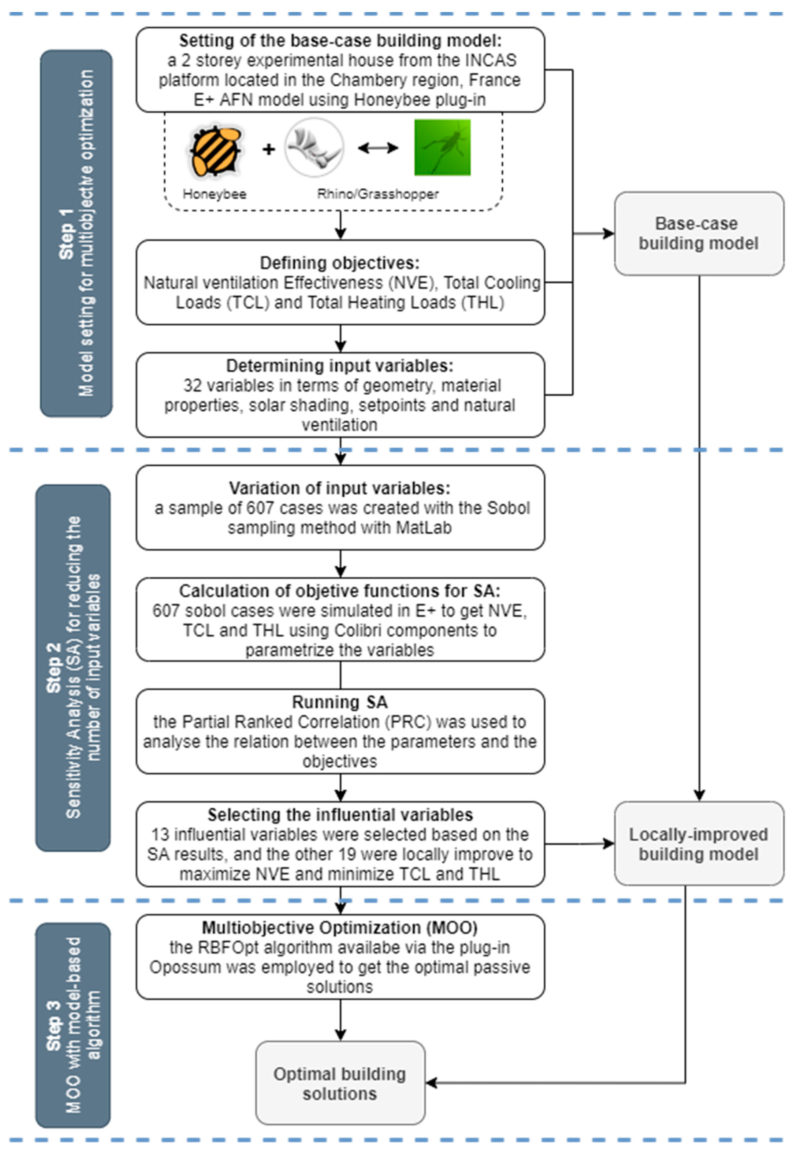
2. Optimization Framework

Following the structure presented in [3], Figure 1 shows this study workflow, divided into three significant steps: model setting with objectives definition, sensitivity analysis, and multiobjective optimization (MOO), which are described in detail in the following sections. Differently from other similar procedures carried out through multiple programs, the approach uses a 3D parametric modeling platform. It allows performing passive design optimization with a single canvas, easing its application into practice.

2.1. Step 1: Model Setting for Multiobjective Optimization

First, an experimental house was parametrically modeled as a base case. With this approach, the modifiable variables are linked to specific architectural elements and forms, enabling direct visualization of these changes, significantly aiding complex geometry design [55]. Thus, different design alternatives can be easily tested in the initial phase, making it possible to find the best solution according to the established goals.

In this study, Rhinoceros was selected as a modeling tool and Grasshopper as a command platform. Honeybee (HB), a plug-in running inside Grasshopper, is used as an engine to perform the energy simulations through EnergyPlus (E+) and Open Studio. A detailed description of the model is provided in Section 3.

2.1.1. Optimization Objectives

• Natural Ventilation Effectiveness (NVE)

The number of hours the outdoor airflows can be used to cool space is estimated through the performance metric Natural Ventilation Effectiveness (NVE) [56], expressed in Equation (1). It calculates the weighted averaged of hourly ratios (${\alpha }_i$) between the available natural ventilation air changes per hour (ACH)—$AC{H}_{avai}$ to the required ones ($AC{H}_{req}$) of zone $i$, where $n$ is the total number of considered building zones, equal to 4.

$$NVE=\raisebox{1ex}{${{\displaystyle \sum }}_{i=1}^n{V}_i{\alpha }_i$}\!\left/ \!\raisebox{-1ex}{${{\displaystyle \sum }}_{i=1}^n{V}_i$}\right. \{\begin{array}{c}\alpha =1, if AC{H}_{avai}\ge AC{H}_{req}\\ \alpha =1, if AC{H}_{req}=0\\ \alpha =0, otherwise\end{array}$$

(1)

$AC{H}_{avai}$ corresponds to the hourly E+ output AFN Zone Infiltration Air Change Rate calculated for the Living room and Bedrooms 1–3, while the $AC{H}_{req}$ is calculated through Equations (2) and (3).

$$AC{H}_{req/min}=\raisebox{1ex}{$3600\times A{F}_{req/min}$}\!\left/ \!\raisebox{-1ex}{$V$}\right.$$

(2)

$$A{F}_{req}=\raisebox{1ex}{$q$}\!\left/ \!\raisebox{-1ex}{$\rho c (T_{comf}-T_{out})$}\right.$$

(3)

where $A{F}_{req}$ is the required airflow to offset cooling load, expressed in m³/s, which is converted to ACH, considering the volume of the room ($V$); $q$ is the heat rate (kj/s) calculated by the energy simulation (air-infiltration, solar radiation, heat gains from people, equipment, and light); $\rho$ is the density of air (kg/m³), set as 1.27; and $c$ is the specific heat capacity of the air (KJ/kg °C), equal to 1050. $T_{comf}$ is used instead of $T_{in}$ because it is assumed that when natural ventilation cannot provide sufficient comfort, occupants rely on mechanical systems. ASHRAE Standard 55 [57] is used at the $T_{comf}$ calculations.

Moreover, the minimum airflow ($A{F}_{min}$) in m³/s is calculated by Equation (4) and converted to ACH by Equation (2), following the design ventilation requirements for the breathing zone of occupiable spaces, according to ASHRAE 62.1 [58].

$$A{F}_{min}=Q_{p}P+Q_{a}A$$

(4)

where $Q_p$ is the outdoor airflow rate required per person, set as 2.5 L/s.person; $P$ is the zone population (the most extensive number of people expected to occupy the zone during typical usage); $Q_a$ is the outdoor airflow rate required per unit area, set as 0.3 L/s·m²; and $A$ is the zone floor area. Minimum and required airflow is compared; therefore, if $AC{H}_{min}$ is greater, it is set as a reference, rather than $AC{H}_{req}$.

In this study, as NVE is evaluated in the living room and bedrooms, the performance metric was measured through the weighted average among the four considered spaces.

• Total Cooling Loads (TCL) and Total Heating Loads (THL)

The building energy demand was separately calculated as the sum of the cooling and heating loads (kWh) of the considered rooms (Living room, Bedrooms 1–3), expressed respectively by Equations (5) and (6) as:

$$TCL={\displaystyle \sum }_{i=1}^n{E}_{ci}$$

(5)

$$THL={\displaystyle \sum }_{i=1}^n{E}_{hi}$$

(6)

where $E_{ci}$ and $E_{hi}$ are E+ outputs from the energy consumption due by the cooling coil and the heat pump for zone $i$ cooling and heating, respectively, and $n$ is the total number of considered zones, equal to 4.

The cooling and heating loads were considered separately since they can be supplied by different energy matrices and present heterogeneous consumption. Therefore, evaluating them together would lead to a limited understanding of their respective demands and solutions.

2.1.2. Input Variables

As this study aims to find optimal passive design solutions for a residential building in a temperate climate in terms of NVE, TCL, and THL, the considered input variables for the reference building involve six variables categories: building orientation, Window-to-Wall Ratio (WWR), opaque and translucid envelope material properties, external window shading, natural ventilation, and HVAC system setpoints and AFN parameters (discharge coefficient and the fraction of glazed area operable). The finally predefined 32 input variables are presented in

Table 2. Input values and their ranges for sensitivity analysis.

Category	Variable Description	Variable Name	Probability Density Function	Base-Case Value	Lower Limit	Upper Limit
Building orientation 1	Building long axis azimuth (o)	x01_orient	Discrete	345	0	315
Window-to-Wall Ratio (WWR)	North WWR (%)	x02_glzRn	Continuous uniform	3.5	3.5	75
	East WWR (%)	x03_glzRe	Continuous uniform	13	3.5	75
	South WWR (%)	x04_glzRs	Continuous uniform	34	3.5	75
	West WWR (%)	x05_glzRw	Continuous uniform	10	3.5	75
Material properties	Window U-value (W/m2K)	x06_windowU	Continuous uniform	1.3	1.05	5.7
	Window Solar Heat Gain Coefficient	x07_shgc	Continuous uniform	0.3	0.21	0.81
	Aerogel thickness (m)	x08_aeroT	Continuous uniform	0.04	0.04	0.12
	Roof thermal conductivity (W/mK)	x09_roofC	Continuous uniform	0.055	0.03	0.15
Window Shade	Opening multiplier factor	x10_shdOp	Continuous uniform	0	0	1
	Fraction of the shade surface open to airflow	x11_shdAir	Continuous uniform	0	0	0.8
	Shading control setpoint—Solar radiation on the window (W/m2)	x12_shdSp	Continuous uniform	0	400	600
SetPoint	Minimum indoor air temperature—AFN ventilation control strategy (°C)	x13_minAirT	Continuous uniform	20	20	22
	Maximum indoor air temperature—AFN ventilation control strategy (°C)	x14_maxAirT	Continuous uniform	27	25	28
	Heating setpoint (°C)	x15_setPoint	Continuous uniform	19	18	19
	Cooling system operation (on-off)	x16_onOff	Discrete	False	True	False
AFN Parameter	Discharge coefficient 2	x17_disCoef	Continuous uniform	0.6	0.33	0.84
Ventilation area x window ratio 3 Fraction of operable glazed area	LWindE Window VWR	x18_LWindE	Continuous uniform	0.75	0.5	1
	LwindS1 Window VWR	x19_LwindS1	Continuous uniform	0.75	0.5	1
	LPorteS2 Window VWR	x20_LPorteS2	Continuous uniform	0.75	0.5	1
	LPorteW Window VWR	x21_LPorteW	Continuous uniform	0.75	0.5	1
	LDoorH Window VWR	x22_LDoorH	Continuous uniform	0.75	0.5	1
	LDoorC Window VWR	x23_LDoorC	Continuous uniform	0.75	0.5	1
	R1WindN Window VWR	x24_R1WindN	Continuous uniform	0.75	0.5	1
	R1WindW Window VWR	x25_R1WindW	Continuous uniform	0.75	0.5	1
	H2W1door Window VWR	x26_H2W1door	Continuous uniform	0.75	0.5	1
	R2WindW Window VWR	x27_R2WindW	Continuous uniform	0.75	0.5	1
	R2WindS Window VWR	x28_R2WindS	Continuous uniform	0.75	0.5	1
	R2Ndoor Window VWR	x29_R2Ndoor	Continuous uniform	0.75	0.5	1
	R3WindE Window VWR	x30_R3WindE	Continuous uniform	0.75	0.5	1
	R3SWind Window VWR	x31_R3SWind	Continuous uniform	0.75	0.5	1
	R3Sdoor Window VWR	x32_R3Sdoor	Continuous uniform	0.75	0.5	1

Note: ¹ The smaller of the angles, measured clockwise, between the true north and the long building axis. ² Measured discharge coefficient values from different window types (Table 3). ³ VWR.

with their respective description, lower and upper limits.

The probability density functions of input variables can affect sensitivity analyses and optimization results. Therefore, although the parameters are intrinsically discrete, they were considered to be continuously uniform, with exception to the building orientation, which is restricted to eight discrete values (from 0–315°, every 45°) and the cooling system operation, defined as true (1) or false (0)—on/off. The range limits of Window U-value and window Solar Heat Gain Coefficient (SHGC) were determined according to the values from the reference building and the available products in the building material market. Regarding the external walls’ thermal performance, the approach adopted was limited to the exterior render thickness, instead of considering a broad thermal conductivity range, as performed with the roof. In this sense, wall composition remains the same, and opaque envelope optimization involves finding the ideal aerogel-based exterior render thickness [59].

Mass flow through openings is directly affected by the wind pressure coefficient ($C_p$), discharge coefficient ($C_d$), and window-opening factor. Each operable opening area was considered individually at this stage to provide a more practical and detailed passive natural ventilation design solution, totaling 14 apertures or subvariables. Similarly, although the literature suggests that $C_d$ values range between 0.60–0.65 for sharp-edged openings [60,61,62], the value can vary depending on the opening porosity, shape, location in the façade, wind angle, and Reynolds number [63]. Therefore, a broader range was considered in the investigation, based on wind-tunnel and on-site assessments.

Table 3. Discharge coefficients/window types for sensitivity analyses.

Window Type		Measured ${\mathit{C}}_{\mathit{d}}$	Source
	Side-hung casement	0.47–0.81	[65]
	Bottom-hung casement
	Tilted 45°	0.45	[66]
	Tilted 90°	0.71
	Holes (open)	0.64
	Holes (closed)	0.06
	Flaps (open)	0.61
	Flaps (closed)	0.24
	Roof	0.25

summarizes the measured discharge coefficients, literature sources, and respective window types. The $C_p$ values are automatically calculated by E+ using the surface average calculation method [64] implemented through the E+ AFN model.

2.2. Step 2: Sensitivity Analyses—Reducing Input Variables Number

Before the optimization, Sensitivity Analyses (SA) were performed to identify the influential passive design variables in terms of the three objective functions previously described in Section 2.1. Implementing SA at the early stage of this study reduced the number of variables for the optimization procedure, improving the algorithm performance and making the process more effective. Tian et al. [67] reviewed sensitivity analysis methods in building energy investigations, which can be local and global. The authors commented which options might be adequate concerning the research purpose, computational cost, number of input variables, and familiarity with the methods. While local SA evaluates the output variability changing one factor at a time, global SA ponders several factors simultaneously, allowing for the interaction between elements, the effect of factor range, and the shape of the factor probability density function to be considered.

To analyze the relationship between the design (or input) parameters on the optimization objective (or output), the “sdo.analyze” function from Simulink^® Design Optimization^TM [33] was implemented in a MatLAB script using the Partial Ranked Correlation (PRC). The global method was chosen because it analyzes how a model parameter and the outputs are correlated, adjusting to remove the other parameters’ effect. First, a sample of 607 cases with raw values (0–1) was generated using the Sobol sampling method. The sample size was defined following the recommendation in [68], which states that the minimum sample size should de 15–19 times the variables number considered in the analysis. Sobol quasirandom sequences are drawn from the probability distributions specified for the parameters, using Equation (7):

$$Va{r}_v=L_{low}+\left(L_{up}-L_{low}\right)\times x$$

(7)

where $Va{r}_v$ is the variable value; $x$ is the raw value, varying from 0 to 1; $L_{low}$ is lower limit; and $L_{up}$ is the upper limit of the variable range. Sampling-based on Sobol’ sequences provides a highly systematic space-filling with low discrepancy, showing a better performance than other sample techniques [69].

The 607 cases were run using Colibri components, a tool that performs parametric simulations distributed with TT Toolbox [70]. A slider controls the case changes, and the resulting impact of each run is recorded into a .csv file. Regarding the simulation time, the 607 runs took around 21 h (≈2 min for simulation) using an Intel i7-7500U Core laptop, up to 3.2 GHz.

2.3. Step 3: Multiobjective Optimization (MOO) with Model-Based Algorithm

Instead of using an evolutionary MOO algorithm, such as HypE [71], SPEA [72], or NSGA-II [73], commonly employed in similar investigations [11,17], the last step uses a Radial Basis Function Multiobjective Optimization (RBFMOpt). This machine-learning-related MOO algorithm won the “Two Objectives Expensive” track of the Black Box Optimization Competition (BBCOMP) 2019 [74]. Moreover, a benchmark study presented in [75,76] showed its good performance compared to other algorithms, finding reasonable solutions with fewer simulations. It has proven efficient and robust, while genetic algorithms perform poorly [77], and therefore was chosen to run this study optimization phase.

In single-objective optimization, the goal is to find a single point, e.g., a design solution, that best answers a sole performance metric or a project requirement. On the other hand, MOO aims to find the best solution points according to multiple conflicting objectives. These points or optimal solutions are non-dominated, meaning that one point’s objectives cannot be improved without harming the others. When connected, the points form a curve, which illustrates the optimization results, known as the Pareto surface or front. According to Ciftcioglu and Bittermann (2009) the Pareto ranking is this solution surface in a multidimensional solution space formed by several criteria, representing the objectives. Although the solutions are diverse on this surface, they are assumed to be valid in an identical way. Thus, the Pareto front graph supports designers’ decision-making since it allows visualization of the trade-off among objectives [78]. In that light, the RBFMOpt’s goal, also known as a model-based method, is to find the nondominated points in the Pareto front. The algorithm builds and iteratively refines surrogate models of the unknown objective function that predict simulation results [79] and approximates the set of points in the solution surface by iterating over a series of weights based on a Halton sequence [80]. Wortmann and Natanian [75] explain that RBFMOpt exploits this property by resuming RBFOpt and feeding it at each iteration with all known points, reweighted according to the up-to-date set of weights. Hence, with every iteration, the initial RBFOpt surrogate model becomes increasingly accurate, leading to more effective optimization cycles. With this approach, model-based optimization is considered an attractive alternative for performance-oriented design [81] because it is seen as particularly effective for optimizing problems with complex associations between variables and objectives and time-expensive simulations [82]. Aimed for BSO Practitioners, the RBFOpt Algorithm Is Available in Grasshopper via the Plug-in Opossum [83].

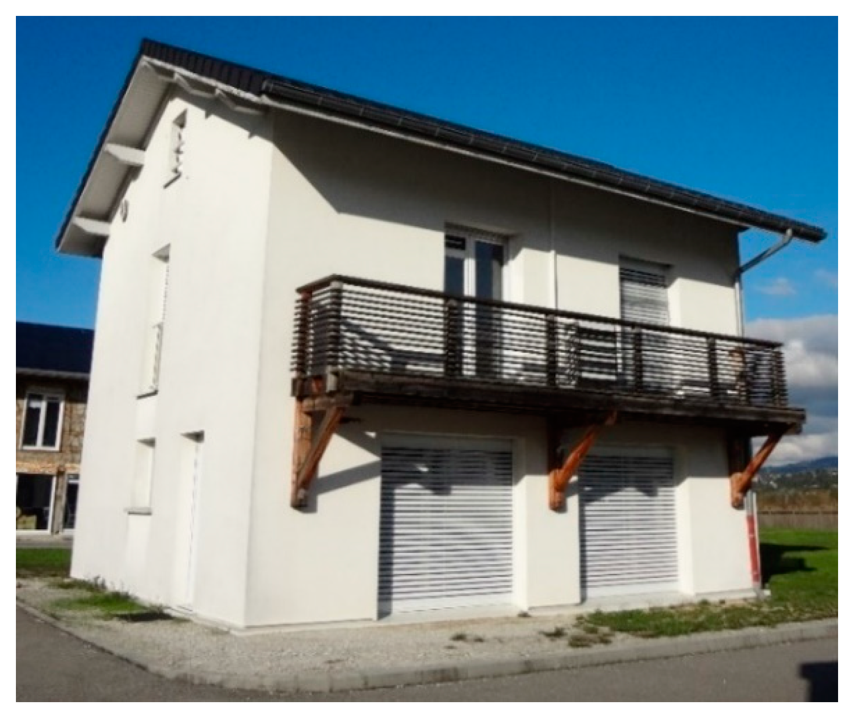
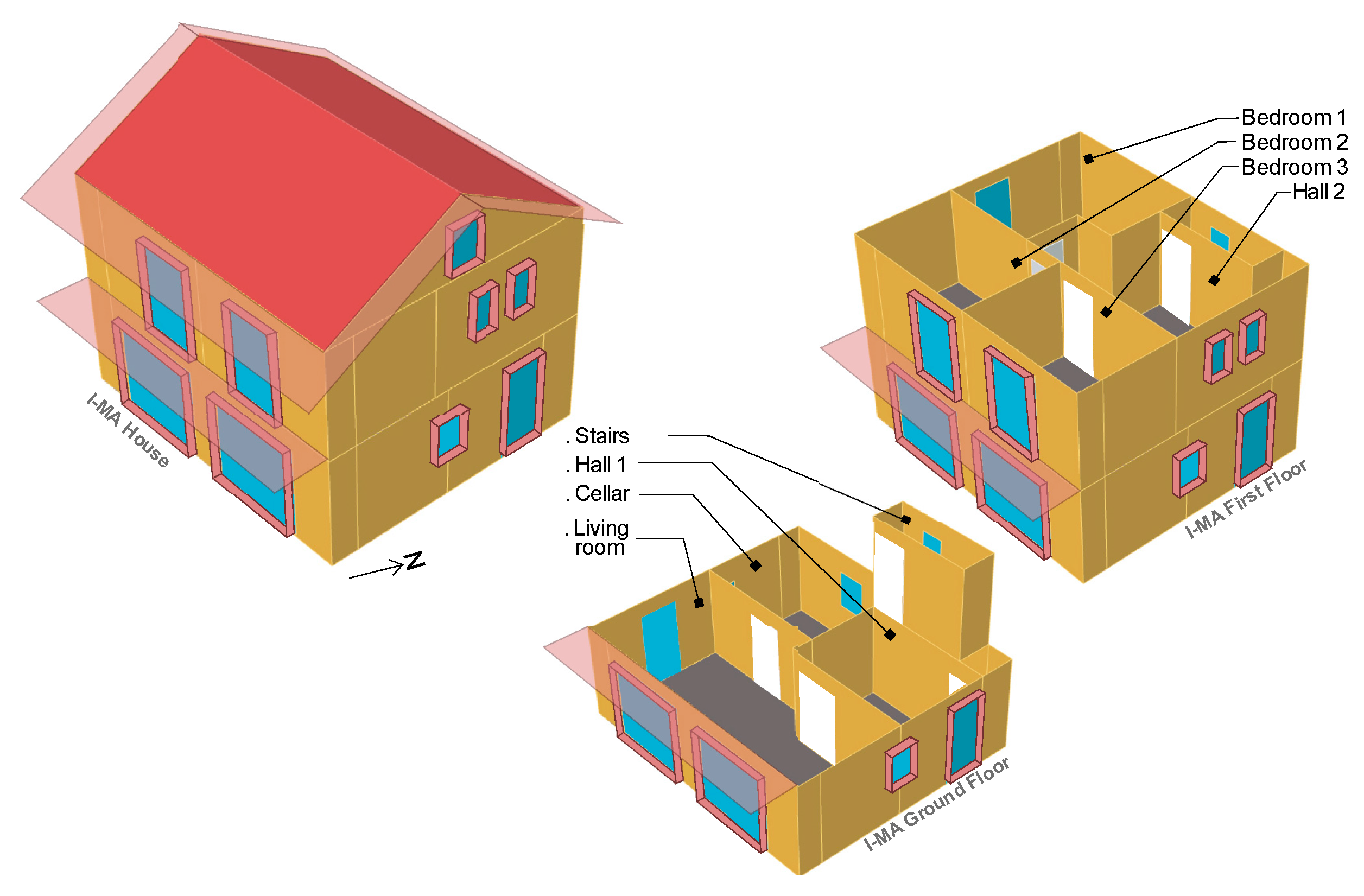
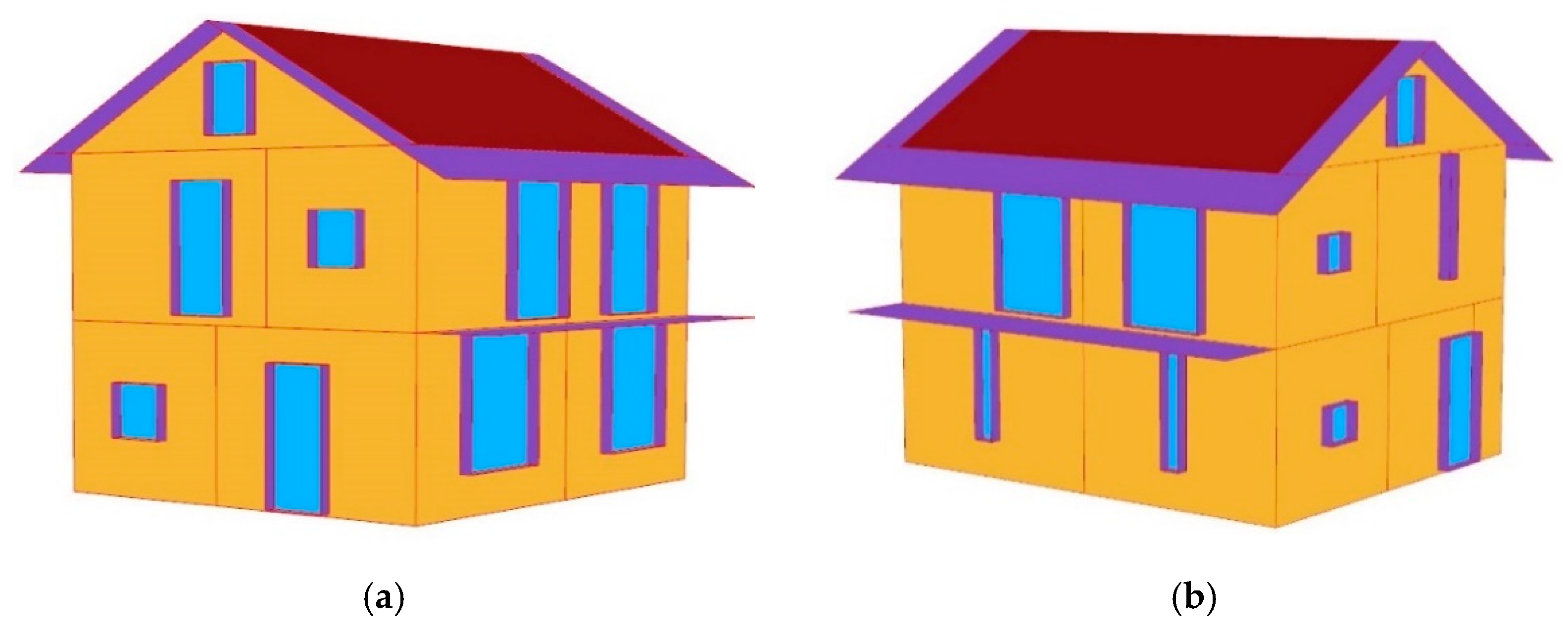
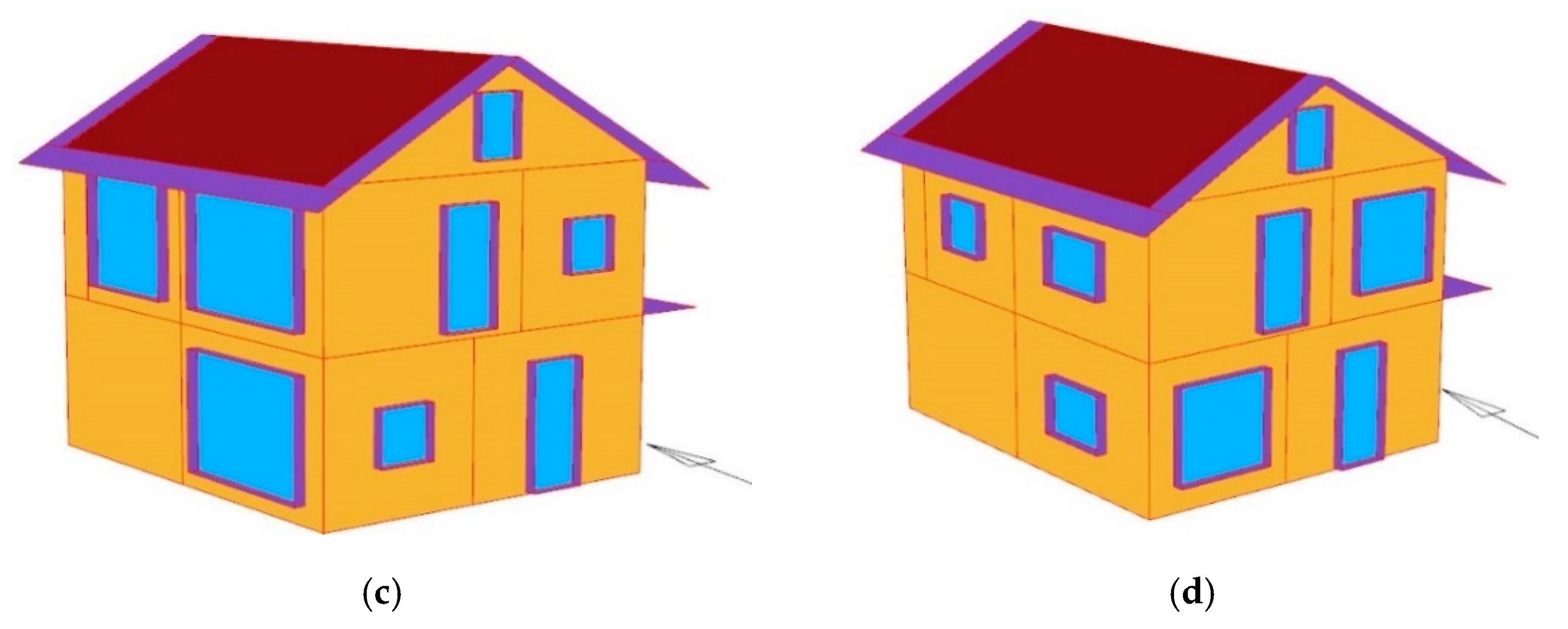
3. Base-Case Building Model

The base-case building (Figure 2) comprises one of the experimental houses from the INCAS platform facility [84,85], developed by the French National Institute for Solar Energy—INES facility located in Bourget-du-Lac, France (45°38′38.5″ N, 5°52′27.4″ E, altitude 270 m). The region is characterized by warm summers (mean and max. temp of 20 and 34 °C), cold and wet winters (mean and min. temp. of 5 and −4 °C), and partly cloudy year-round (Köppen: temperate climate, warm summer—Cfb [86]). The reference building, also known as I-MA house, is a low-energy two-story rectangular construction (7.5 × 8.5 m), with an opaque envelope made of cavity bricks (42 cm thick) covered with an aerogel-based exterior insulating rendering. The building is taken as a base case in this study because one of its purposes is to assist numerical validations, being equipped with numerous sensors and featuring a simple design, which favors simulation process and verification. Moreover, it is a passive building [87], whose design represents a single-family residence typically found in the region. Passive Houses have been expanding in the market, as they present themselves as a solution to the challenges related to energy efficiency [88,89,90]. In this sense, the base building is also representative and characterizes a movement, at least in Europe, to build under strict energy standards.

Based on a one-week monitoring campaign (19–25 August 2014), an E+ numerical model was created, calibrated, and used to perform annual energy and natural ventilation assessments in [91,92], which also provide a detailed description of the measurement equipment, experimental protocol, construction, and the climatic data recorded on-site and used at the simulation. Moreover, the complete settings of the E+ model, including the occupancy schedule and the .idf file, are available in the Data in Brief article [93].

Model creation within the optimization framework begins by importing the .idf file available in [93] using the Honeybee component HB_Import idf. The base-case building geometry is translated into the 3D modeling parametric platform (Rhino + Grasshopper) through HB-Energy components. Figure 3 shows the nine thermal zones modeled with the HB Model: three on the ground (Living room, Cellar, Hall 1), four on the first floor (Bedrooms 1–3, Hall 2), and an attic and a staircase zone. Natural ventilation can be used as a cooling strategy in all zones; therefore, the openings, either windows or external/internal doors, were modeled as AirflowNetwork (AFN) objects. However, just the Living room and the Bedrooms have HVAC system, modeled with the HB Apply Setpoint Values component that uses the E+ Ideal Loads Air System.

The external openings, either windows or doors, were assumed to have parametrically adjustable dimensions. Their size varies in a window-to-wall-ratio function using the HB Apertures by Ratio component, which depends on façade orientation (HB Façade Parameters). Moreover, external shading devices were modeled with the HB Window Construction Shade component, controlled based on the solar radiation incidence on the window, with a parametric setpoint varying from 400–600 W/m².

Openings operation regarding natural ventilation and building’s heating/cooling system was established, configuring a hybrid behavior. Ventilation control depends on occupancy and was based on a temperature setpoint, which was parametrized and varied from 20–22 °C. The living room apertures can be operated only when the room is occupied, whereas the bedrooms’ windows are operable whenever someone is in the house. Regarding the heating system control, its activation happens if the occupied room’s operative temperature is below 18–19 °C (parameterized value) so that the indoor temperature is maintained at 21 °C. Once in operation, the heater is only turned off when the occupancy in the room is null, and whenever the windows are open, mechanical ventilation cannot happen, as well as the contrary.

Moreover, an extra operational condition was considered to turn on the cooling system in the conditioned spaces when natural ventilation is insufficient to maintain the indoor temperature within the established parameterized limited (25–28 °C). This hybrid behavior was modeled through the Energy Management System (EMS) object [94] by adding additional strings to the HB Model to OpenStudio Model component. The controls developed in the EMS are presented in [93].

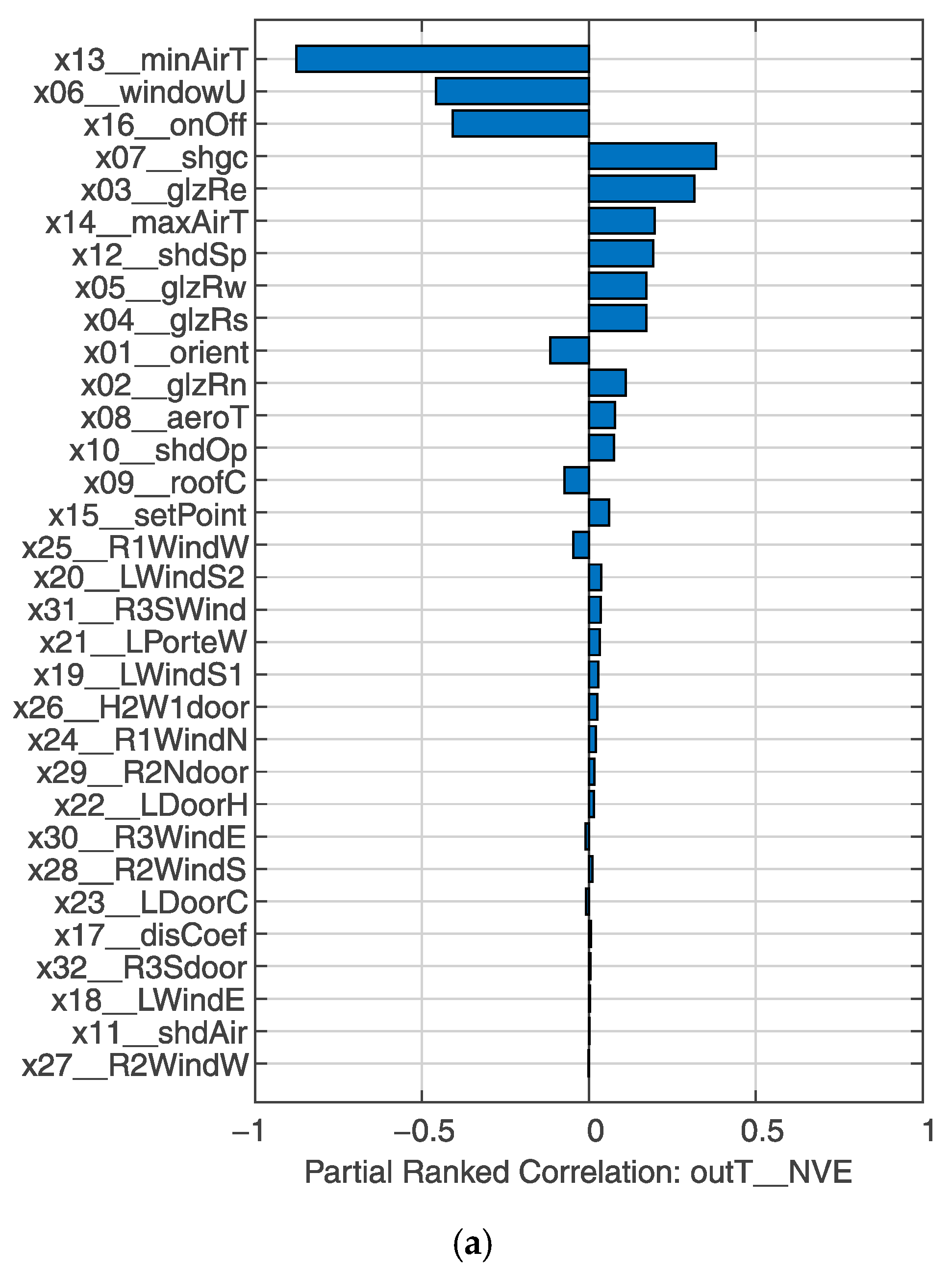
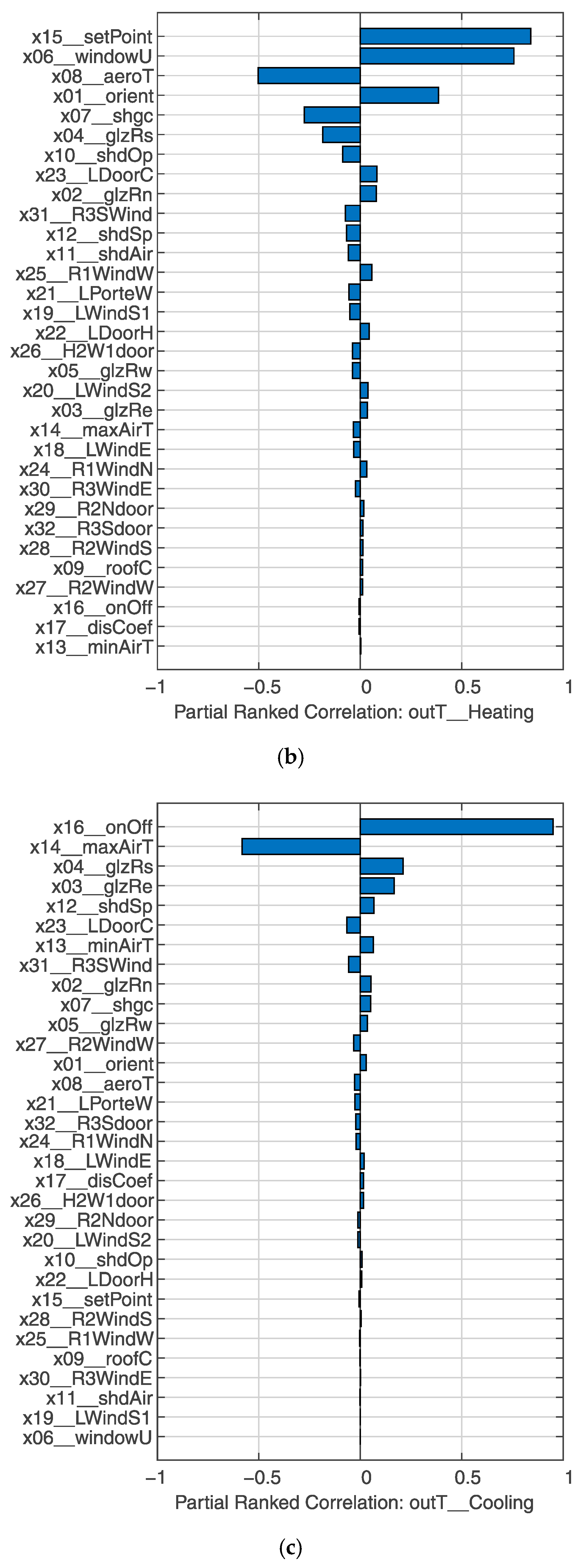
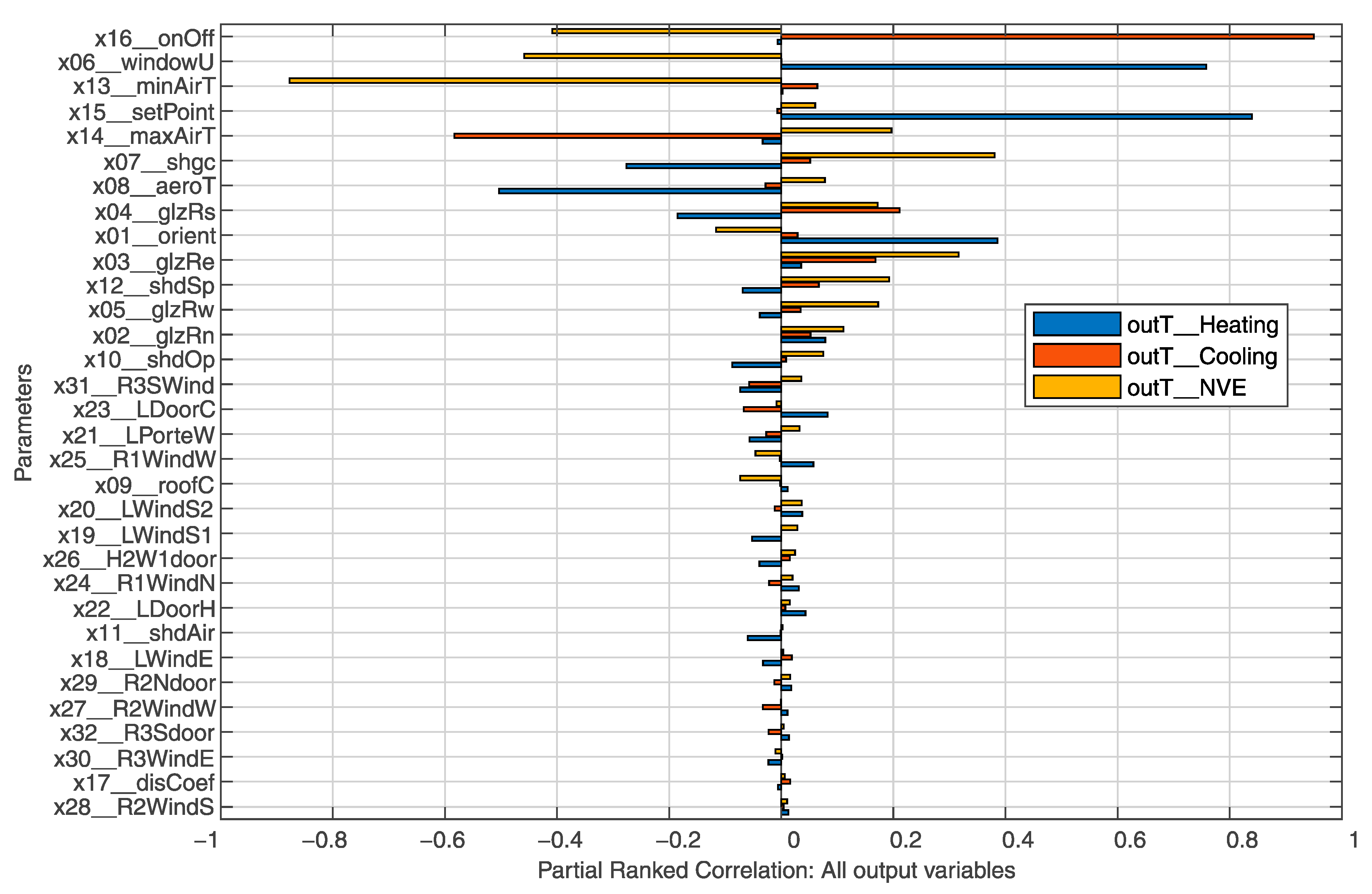
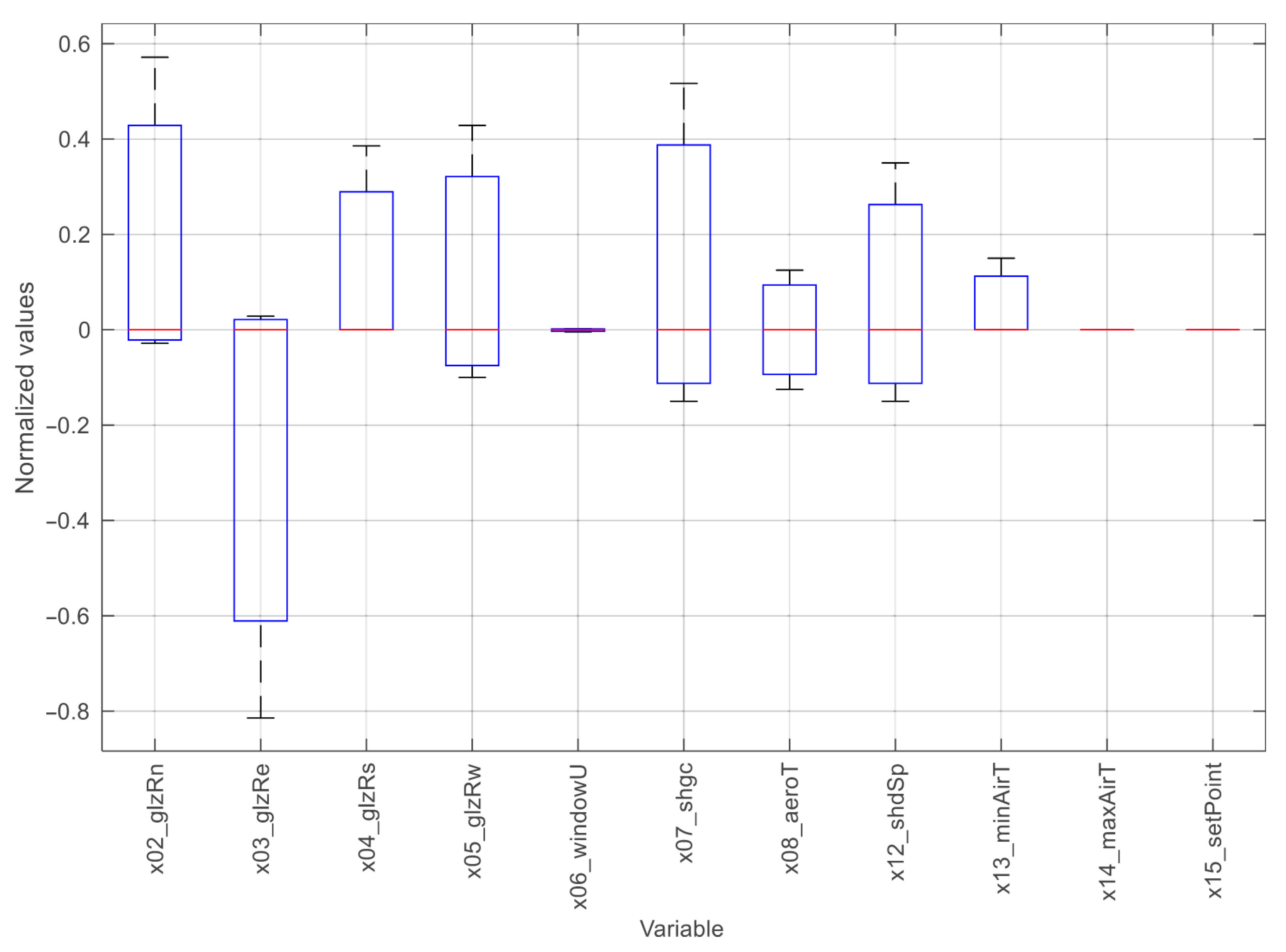
4. Selection of the Influential Variables and Sensitivity Analyses Results

The relation between the design parameters on the outputs was analyzed through the Partial Ranked Correlation so that the most influential variable could be determined. With this approach, the performance of the radial-based algorithm can be improved, and the search for optimal solutions is therefore enhanced.

Figure 4 shows the calculated PRC of the 32 variables for the three objectives (NVE, TCL, and THL), sorting from the largest to the smallest absolute value. The higher the PRC absolute value, the more influential variable. The PRC positive/negative value indicates the proportional/inverse relationship between an input parameter and the outputs.

The figures show that the order and magnitude of the input variables slightly diverge between the three objectives. Based on the PRC analysis, half of the top 10 influential variables for the three objectives overlapped.

Table 4. Results of sensitivity analysis and locally-improvements for the remaining less influential variables.

Variable Description	Variable Name	PCR for NVE (Ranking)	PCR for TCL (Ranking)	PCR for THL (Ranking)	Locally-Improved Solution
Building long axis azimuth (o)	x01_orient	Negative (10)	Positive (13)	Positive (04)
North WWR (%)	x02_glzRn	Positive (11)	Positive (09)	Positive (09)
East WWR (%)	x03_glzRe	Positive (05)	Positive (04)	Positive (20)
South WWR (%)	x04_glzRs	Positive (09)	Positive (03)	Negative (06)
West WWR (%)	x05_glzRw	Positive (08)	Positive (11)	Negative (18)
Window U-value (W/m2K)	x06_windowU	Negative (02)	Positive (32)	Positive (02)
Window Solar Heat Gain Coefficient	x07_shgc	Positive (04)	Positive (10)	Negative (05)
Aerogel thickness (m)	x08_aeroT	Positive (12)	Negative (14)	Negative (03)
Roof thermal conductivity (W/mK)	x09_roofC	Negative (14)	Negative (28)	Positive (28)	base-case
Opening multiplier factor	x10_shdOp	Positive (13)	Positive (23)	Negative (07)	HB E+ default
Fraction of the shade surface open to airflow	x11_shdAir	Positive (31)	Negative (30)	Negative (12)	minimum
Shading control setpoint—Solar radiation on the window (W/m2)	x12_shdSp	Positive (07)	Positive (05)	Negative (11)
Minimum indoor air temperature—AFN ventilation control strategy (°C)	x13_minAirT	Negative (01)	Positive (07)	Positive (32)
Maximum indoor air temperature—AFN ventilation control strategy (°C)	x14_maxAirT	Positive (06)	Negative (02)	Negative (21)
Heating setpoint (°C)	x15_setPoint	Positive (15)	Negative (25)	Positive (01)
Cooling system operation (on-off)	x16_onOff	Negative (3)	Positive (01)	Negative (30)
Discharge coefficient	x17_disCoef	Positive (28)	Positive (19)	Negative (31)	minimum
LWindE Window VWR	x18_LWindE	Positive (30)	Positive (18)	Negative (22)	base-case
LwindS1 Window VWR	x19_LwindS1	Positive (20)	Negative (31)	Negative (15)	base-case
LPorteS2 Window VWR	x20_LPorteS2	Positive (17)	Negative (22)	Positive (19)	base-case
LPorteW Window VWR	x21_LPorteW	Positive (19)	Negative (15)	Negative (14)	base-case
LDoorH Window VWR	x22_LDoorH	Positive (24)	Positive (24)	Positive (16)	base-case
LDoorC Window VWR	x23_LDoorC	Positive (27)	Negative (06)	Positive (08)	base-case
R1WindN Window VWR	x24_R1WindN	Positive (22)	Negative (17)	Positive (23)	base-case
R1WindW Window VWR	x25_R1WindW	Negative (16)	Negative (27)	Positive (13)	base-case
H2W1door Window VWR	x26_H2W1door	Positive (21)	Positive (20)	Negative (17)	base-case
R2WindW Window VWR	x27_R2WindW	Negative (32)	Negative (12)	Positive (29)	base-case
R2WindS Window VWR	x28_R2WindS	Positive (26)	Positive (26)	Positive (27)	base-case
R2Ndoor Window VWR	x29_R2Ndoor	Positive (23)	Negative (21)	Positive (25)	base-case
R3WindE Window VWR	x30_R3WindE	Positive (25)	Positive (29)	Negative (24)	base-case
R3SWind Window VWR	x31_R3SWind	Positive (18)	Negative (08)	Negative (10)	base-case
R3Sdoor Window VWR	x32_R3Sdoor	Negative (29)	Negative (16)	Positive (26)	base-case

Note: The bold items are less influential variables and are supposed to be locally improved.

shows the sensitivity analysis results straightforwardly, illustrating the relationships between each input variable and the three goals (i.e., positive or negative) and each input variable’s sensitivity ranking.

Based on these results and aiming to reduce the input variables number, Figure 5 shows the PRC’s sum for the three objectives, sorting the numbers according to their absolute value and finding a new arrangement index.

Lastly, the influential variables regarding all objectives were screened out to be analyzed in the next optimization step, keeping the balance between the three considered goals. The finally selected parameters are listed in

Table 5. Input variables and their ranges for multiobjective optimization.

Variable Description	Variable Name	Probability Density Function	Base-Case Value	Locally Improved Values	Lower Limit	Upper Limit
Building long axis azimuth (o)	x01_orient	Discrete	345		0	315
North WWR (%)	x02_glzRn	Continuous uniform	3.5		3.5	75
East WWR (%)	x03_glzRe	Continuous uniform	13		3.5	75
South WWR (%)	x04_glzRs	Continuous uniform	34		3.5	75
West WWR (%)	x05_glzRw	Continuous uniform	10		3.5	75
Window U-value (W/m2K)	x06_windowU	Continuous uniform	1.3		1.05	5.7
Window Solar Heat Gain Coefficient	x07_shgc	Continuous uniform	0.3		0.21	0.81
Aerogel thickness (m)	x08_aeroT	Continuous uniform	0.04		0.04	0.12
Roof thermal conductivity (W/mK)	x09_roofC	Continuous uniform	0.055	0.055
Opening multiplier factor	x10_shdOp	Continuous uniform	0	0.5
Fraction of the shade surface open to airflow (permeability)	x11_shdAir	Continuous uniform	0	0
Shading control setpoint—Solar radiation on the window (W/m2)	x12_shdSp	Continuous uniform	0		400	600
Minimum indoor air temperature—AFN ventilation control strategy (°C)	x13_minAirT	Continuous uniform	20		20	22
Maximum indoor air temperature—AFN ventilation control strategy (°C)	x14_maxAirT	Continuous uniform	27		25	28
Heating setpoint (°C)	x15_setPoint	Continuous uniform	19		18	19
Cooling system operation (on-off)	x16_onOff	Discrete	False	True
Discharge coefficient	x17_disCoef	Continuous uniform	0.5	0.6
LWindE Window VWR	x18_LWindE	Continuous uniform	0.75	0.75
LwindS1 Window VWR	x19_LwindS1	Continuous uniform	0.75	0.75
LPorteS2 Window VWR	x20_LPorteS2	Continuous uniform	0.75	0.75
LPorteW Window VWR	x21_LPorteW	Continuous uniform	0.75	0.75
LDoorH Window VWR	x22_LDoorH	Continuous uniform	0.75	0.75
LDoorC Window VWR	x23_LDoorC	Continuous uniform	0.75	0.75
R1WindN Window VWR	x24_R1WindN	Continuous uniform	0.75	0.75
R1WindW Window VWR	x25_R1WindW	Continuous uniform	0.75	0.75
H2W1door Window VWR	x26_H2W1door	Continuous uniform	0.75	0.75
R2WindW Window VWR	x27_R2WindW	Continuous uniform	0.75	0.75
R2WindS Window VWR	x28_R2WindS	Continuous uniform	0.75	0.75
R2Ndoor Window VWR	x29_R2Ndoor	Continuous uniform	0.75	0.75
R3WindE Window VWR	x30_R3WindE	Continuous uniform	0.75	0.75
R3SWind Window VWR	x31_R3SWind	Continuous uniform	0.75	0.75
R3Sdoor Window VWR	x32_R3Sdoor	Continuous uniform	0.75	0.75

, and the locally improved values are established for the less influential parameters. All 12 remained variables presented a PRC absolute result bigger than 0.1. The number of parameters could be drastically reduced because many had a low impact on objective functions, such as all those related to Ventilation area x Window Ratio (VWR). Adopting a unique value for such parameters makes the optimization problem more effective.

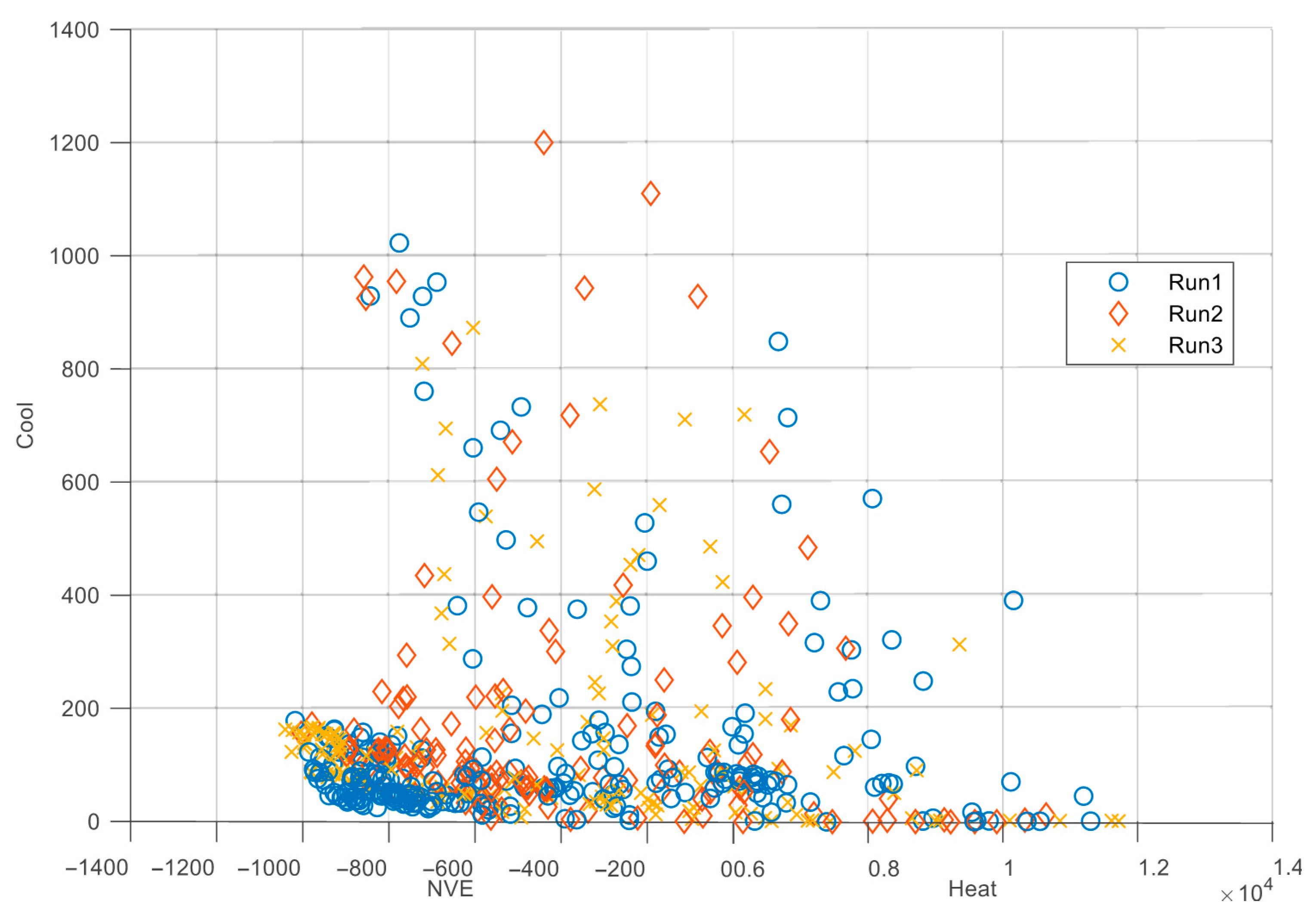
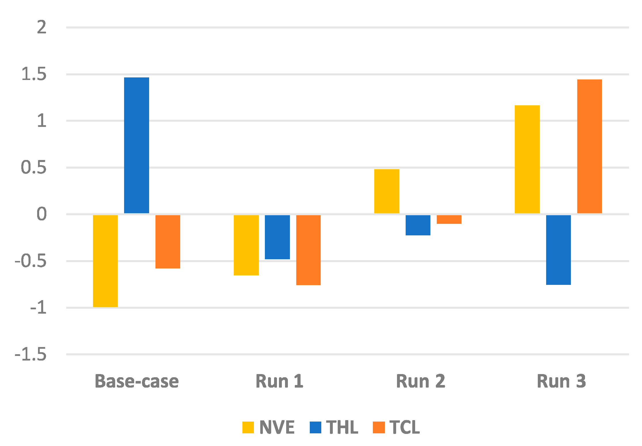
5. MOO through RBFMOpt

In this step, the goal was to find the optimal values of the 12 selected influential passive design parameters for maximizing cooling ventilation (NVE) while minimizing the building energy demand (THL and TCL).

Although more than forty parameters control the RBFOpt, the Opossum’s graphical user interface reduces its complexity into three tabs that afford increasing the control levels and offers presets based on intensive testing with mathematical test functions [76].

Table 6. Adopted settings with the Opossum optimization process.

Configuration	Description	Input Data
Optimization type	One is limited to either minimize or maximize the objective functions. If controversial, the one to be adjusted is multiplied by −1.	Minimize
Algorithm	Algorithm chosen from those available in the plug-in	RBFOpt
Max iterations	Stop the simulation if the iterations exceed this number	500
Number of optimizations runs	Number of times the simulations will be repeated	3
Number of cycles	Determines how long the algorithm spends optimizing each set of weights	6

shows the adopted settings within Opossum in the optimization runs (Run 1, Run 2, and Run 3). Most of them were left as default, following the predetermined plug-in configurations.

Each variable is modeled in the Grasshopper canvas with a number slider, floating the value according to the predetermined lower and upper limits. Opossum saves each interaction run in a single log file, and after performing all function evaluations, it summarizes the results in a table, which makes it easy to revisit all optimization outcomes by double-clicking the entries in it. Among the results is the hypervolume from each simulation, which measures the objective space’s volume dominated by the set of points, e.g., design solutions [75]. Within MOO, the hypervolume must be maximized as all objectives are to be minimized. The goal is to dominate as much of the objective space as possible since, mathematically, if one set is better than the other, it spans a larger hypervolume [95].

The former procedures resulted in Figure 6, which shows a 3D representation of the three optimization objectives results. Each run generated respectively 268, 147, and 168 cases, totaling 588 function evaluations or model regenerations. It took about 20 h to run them all, with the same laptop configurations mentioned in item 0. The Pareto front is depicted in Figure 7, where the best solutions found in each run can be observed at the curve formed at the lower-left corner.

The hypervolume calculated in each of the three runs is the metric used to find the optimized solution. In this regard, Figure 8 groups the three runs according to the hypervolume generated, which shows stability (convergence) of the results between 100 and 150 interactions. The numbers in the graph correspond to the NVE, TCL, and THL results of the three runs’ optimal solutions, which are also summarized in

Table 7. Range of optimization variables in base-case and RBFOpt solutions and their respective objective functions results.

Selected Influential Variables	Variable Name	Base-Case	Ranges	Run 1	Run 2	Run 3
Building long axis azimuth (o)	x01_orient	345	(0.315)	315	90	90
North WWR (%)	x02_glzRn	3.5	(5.75)	17	57	15
East WWR (%)	x03_glzRe	13	(5.75)	5	62	64
South WWR (%)	x04_glzRs	34	(5.75)	7	7	34
West WWR (%)	x05_glzRw	10	(5.75)	5	12	42
Window U-value (W/m2K)	x06_windowU	1.3	(1.05, 5.7)	1.09	1.08	1.06
Window Solar Heat Gain Coefficient	x07_shgc	0.3	(0.21, 0.81)	0.39	0.30	0.70
Aerogel thickness (m) Wall U-value (W/m2K)	x08_aeroT	0.04 0.71	(0.04, 0.12) (0.71, 0.26)	0.12 0.26	0.10 0.31	0.11 0.28
Shading control setpoint—Solar radiation on the window (W/m2)	x12_shdSp	0	(400, 600)	590	490	520
Minimum indoor air temperature—AFN ventilation control strategy (°C)	x13_minAirT	20	(20, 22)	20.3	20	20
Maximum indoor air temperature—AFN ventilation control strategy (°C)	x14_maxAirT	27	(25, 28)	28	28	28
Heating setpoint (°C)	x15_setPoint	19	(18, 19)	18	18	18
NVE		585		665	933	1096
THL		11.238		7.924	8.359	7.455
TCL		10		4	26	78

.

Moreover, Figure 9 allows a comparison of these results variability over the runs, presenting their normalized values, while Figure 10 illustrates normalized values, but of the parameters of RBFOpt solutions according to the ranges.

Additionally, Figure 11 shows the respective optimized geometry generated for the three runs’ selected solutions (Figure 11b–d) and the base case (Figure 11a). The images are automatically generated with the Honeybee component HB Visualyze by Type and show the changes related to building orientation and openings size. Thus, the significant WWR variations that were firstly numerically attested are also visualized.

In sum, when comparing all runs to the base case, an improvement between 14–87% and 26–34% occurs in NVE and THL, respectively. As for TCL, a reduction of 60% concerning the reference is restricted to Run 1, with an increase of 160% for Run 2 and 680% in Run 3. Nevertheless, cooling consumption presents nearly negligible values. Thus, turning on the air conditioning system can be disregarded, meaning that the I-MA building can rely on cooling natural ventilation during the warm seasons.

6. Discussion

A fast convergence can be noted regarding the number of runs presented in Figure 8 (less than 150 interactions). Finding optimal solutions with few simulations is one of the RBFMOpt algorithm advantages pointed in benchmark studies [75,76] when compared to other algorithms. Observing the object function results individually in Figure 8, the total heat loads (THL) present a slight variation in all runs, ranging from 7455 to 8359 kWh. Regarding the objectives related to natural ventilation, NVE, and total cooling loads (TCL), the values show more significant variability, ranging from 665 to 1096 h/year for NVE and from 4 to 78 kWh for TCL. Simultaneously, there is a direct relationship between these two results, where the greater the number of NVE hours, the greater the energy consumption due to cooling (TCL). By contrast, such association is not observed among the heating loads and other objectives.

When analyzing each of the variable outcomes for the optimal alternatives, the building long axis azimuth (x01) presents for runs 2 and 3 θ = 90°, while Run 1 has θ = 315°, representing a minor difference regarding the base case. On the other hand, in all solutions, the long axis changes so that the façades are more exposed. The base case has a north–south orientation, where the south façade is the one with the most significant solar incidence and the one with the most extensive opening area. When observing the three optimized solutions, solar distribution is more balanced among the façades, which also have different WWR. Thus, it is evident that with a heterogeneous distribution of the glazed areas, the proposed implantation in the optimized solutions enhances the solar gains through the different building translucent facades.

On the other hand, compared to the base-case values (Figure 9), the optimized solutions show a clear improvement in NVE and THL of all runs and for TCL in Run 1. The NVE-bars show an increasing behavior for all runs, but the THL-bars show a decreasing one. As for the TCL, on the other hand, the bars only diminish in run 1.

Besides showing the objective results for each run, Table 6 also outlines the scope of the optimization variables from both base case and optimal solutions. Figure 10 presents the solution variables, except for the building orientation, within a box plot graph with normalized values centered on median 0, allowing for a direct results’ correlation.

Some parameters show a low variation, while others present a high range. Wortmann [76] comments in this regard that repeated runs of stochastic algorithms for identical settings and problems can have very different results. In this sense, parameters related to the temperature and shading setpoints, aerogel thickness, and window U-Value present more cohesive results, while geometric variables are more dispersed. Therefore, it can be seen that concerning the physical properties, the values remain within a narrow range. On the other hand, the variables related to the building shape and form welcomed more alternatives, presenting a wider variance. As a result, during the early design stages, the variables associated with the physical properties could be restricted to a known range, focusing the search for optimized solutions on the geometric aspects.

With considerable discrepancies, the four WWRs (x02, x03, x04, and x05) vary significantly in all runs, where Run 1 presents the closest values to the base case, which is reflected in the objective function’s outputs. Similarly, bigger WWRs lead to a higher NVE and TCL, which is the Run 3 case. On the other hand, the same Run also presents the lowest heating consumption (THL). That is because the Window U-values (x06) remained within small values, allowing solar entry with low thermal losses in periods without radiation. In high Window U-values, oversized windows would negatively impact heating loads since the opaque/isolated surfaces would decrease, and the losses due to a low-performance glass could surpass solar gains.

Moreover, concerning the insulating thickness (x08), its value in Run 3 was not the largest one found, at 11 cm, while Run 1 remains with the maximum range, 12 cm, and still had a greater THL. In this sense, the aerogel layer’s optimized values were left between 10 and 12 cm, more than double compared to the base case. When converting the corresponding thickness values (cm) to Wall U-values (W/m²K), the wall thermal transmittance varies from 0.71–0.26 W/m²K, for an aerogel thickness of 4–12 cm, respectively. The Wall U-Value found in Run 2 and 3 correspond to 0.31 W/m²K and 0.28 W/m²K. Therefore, when relating the Walls and Windows U-values for the three solutions, a inversely proportional relationship is perceived in Run 1, where the transparent surface presents the worst performance and the opaque surface the best. However, this is not the case for Run 2 or 3, although both values are close. Nonetheless, a relationship between the different envelope systems (opaque vs. translucid) is observed, which seeks to compensate each other to achieve the desired building performance.

No clear relationship was observed between the SHGC (x07) and Window U-value (x06) variables. The Window U-value shows a slight variance while SHGC presents a broader range. Run 3 has both the best Window U-value and the worst SHGC, which might indicate compensation, but it is not the case with the other two solutions.

Furthermore, Table 6 results show that the setpoint temperatures are at their limit and that the minimum (x13) and maximal (x14) optimized air temperatures for natural ventilation represent their respective lowest and highest possible values. Likewise, the heating setpoint (x15) stays within its lower limit. This low variance and even constancy are also observed in Figure 10, showing that the temperature range for the window’s operation resulted in a good NV performance (20–28 °C). On the other hand, setting a higher upper limit, bis 31 °C for instance, might also be acceptable and could be considered, as exposed in studies in hot and humid climates [96,97,98].

Concerning the shading control setpoint (x12), a stochastic relationship is also found when analyzing the optimization variables and the objectives outputs. Nonetheless, the variables interval among the solutions remains within a smaller dimension (490–590 W/m²) than the initial range (400–600 W/m²). Thus, the search space is limited, easing local parameter improvement.

As a final comment, the optimized configurations of Figure 11 could be replicable in similar buildings under the same climatic conditions or used as a starting point when performing analogous studies. In this way, local improvements can be implemented by restricting the variables number with reference values, thus preoptimizing the solutions.

Lastly, designing on a parametric platform makes it easier to handle the numerous geometric variables of a project, which is one of the challenges when proposing high-performance solutions. Therefore, the approach is an uncomplicated way to deal mainly with the building shape and experiment with various alternatives to find the one that best fits the proposed objectives.

7. Conclusions

This study uses parameterization, simulation, sensitivity analyses, and optimization tools applied to a residential building, set as a reference case. An optimization framework is introduced, employing a parametric 3D modeling platform and a radial-based algorithm. Moreover, the paper presents a brief review of performance-based design combined with building simulation and optimization. It evidenced the use of the same program in project development as a user-friendly alternative to integrate the concept of Multiobjective Optimization (MOO) into the design process.

Sensitivity Analysis (SA) was performed before the optimization step in an addendum to the one-software approach, given the variables under investigation. Thus, the algorithm performance could be improved, enhancing the search for the optimal solutions to build.

Among the main conclusions concerning the SA and optimization outcomes, it is highlighted that:

• The influential variables identified in SA analyses depended on the objective considered, showing different ranks among the three established metrics: Natural Ventilation Effectiveness (NVE), Total Heating Loads (THL), and Total Coaling Loads (TCL). However, an overall perspective identified those with the most impact as the setpoint temperatures that regulated natural ventilation or mechanical systems activation. On the other hand, although considered relevant for openings design, the parameter about the ventilation area provided smaller contributions. Therefore, together with the less influential variables, it was locally improved;
• MOO results showed a direct relationship between the size of the windows, NVE, and TCL, which does not apply to THL. The building envelope’s thermal transmittance showed a more significant impact for the heating loads (THL), and all optimized solutions had low U-values for both opaque and transparent surfaces. Given these differences, the complexity of multiobjective problems is evidenced, and the optimization stage can be considered an ally when developing high-performance buildings;
• The model-based algorithm (RBFMOpt) used at the optimization step showed performance consistent with that presented in the benchmark studies, converging with a low number of interactions. Therefore, its application in time-intense simulation investigations is endorsed;
• Findings concerning the physical and geometric variables range could be applied in similar studies, limiting the parameters related to material properties and increasing those about geometry. The optimization results showed that the geometric aspects provided a greater solution diversity among the variables investigated in this work.
• Regarding the framework adopted in this research, the following aspects can be stressed.
• Modeling through a 3D parametric platform allows for the manipulating of numerous variables, being especially effective when dealing with geometric parameters;
• Performing all processes through a single software reduces uncertainties and provides a more straightforward workflow, which facilitates control and implementation;
• The approach is suitable for early project stages because architects and designers would be more receptive and better instrumented to apply MOO, encouraging passive strategies implementation when using such tools.

Finally, future research could include testing different algorithms to evaluate their performance and differences between the optimized solutions. Such investigations can support studies and applications related to performance-based design, helping to consolidate the approach.

References

1. European Commission. Communication from the Commission to the European Parliament, the Council, the European Economic and Social Committee and the Committee of the Regions: A Policy Framework for Climate and Energy in the Period from 2020 Up to 2030, Brussels. 2014. Available online: https://eur-lex.europa.eu/legal-content/EN/TXT/PDF/?uri=CELEX:52014DC0015&from=EN (accessed on 13 September 2020).
2. Yu, W.; Li, B.; Jia, H.; Zhang, M.; Wang, D. Application of multi-objective genetic algorithm to optimize energy efficiency and thermal comfort in building design. Energy Build. 2015, 88, 135–143. [Google Scholar] [CrossRef]
3. Gou, S.; Nik, V.M.; Scartezzini, J.-L.; Zhao, Q.; Li, Z. Passive design optimization of newly-built residential buildings in Shanghai for improving indoor thermal comfort while reducing building energy demand. Energy Build. 2018, 169, 484–506. [Google Scholar] [CrossRef]
4. Méndez Echenagucia, T.; Capozzoli, A.; Cascone, Y.; Sassone, M. The early design stage of a building envelope: Multi-objective search through heating, cooling and lighting energy performance analysis. Appl. Energy 2015, 154, 577–591. [Google Scholar] [CrossRef]
5. Huang, K.-T.; Hwang, R.-L. Parametric study on energy and thermal performance of school buildings with natural ventilation, hybrid ventilation and air conditioning. Indoor Built Environ. 2016, 25, 1148–1162. [Google Scholar] [CrossRef]
6. Nguyen, A.-T.; Reiter, S.; Rigo, P. A review on simulation-based optimization methods applied to building performance analysis. Appl. Energy 2014, 113, 1043–1058. [Google Scholar] [CrossRef]
7. Westermann, P.; Evins, R. Surrogate modelling for sustainable building design—A review. Energy Build. 2019, 198, 170–186. [Google Scholar] [CrossRef]
8. Chen, X.; Yang, H.; Zhang, W. Simulation-based approach to optimize passively designed buildings: A case study on a typical architectural form in hot and humid climates. Renew. Sustain. Energy Rev. 2018, 82, 1712–1725. [Google Scholar] [CrossRef]
9. Bradner, E.; Iorio, F.; Davis, M. Parameters tell the design story: Ideation and abstraction in design optimization. In Proceedings of the SimAUD 2014, Symposium on Simulation for Architecture and Urban Design, Tampa, FL, USA, 13–16 April 2014. [Google Scholar]
10. Shi, X.; Tian, Z.; Chen, W.; Si, B.; Jin, X. A review on building energy efficient design optimization rom the perspective of architects. Renew. Sustain. Energy Rev. 2016, 65, 872–884. [Google Scholar] [CrossRef]
11. Hamdy, M.; Nguyen, A.-T.; Hensen, J.L.M. A performance comparison of multi-objective optimization algorithms for solving nearly-zero-energy-building design problems. Energy Build. 2016, 121, 57–71. [Google Scholar] [CrossRef] [Green Version]
12. Bre, F.; Silva, A.S.; Ghisi, E.; Fachinotti, V.D. Residential building design optimisation using sensitivity analysis and genetic algorithm. Energy Build. 2016, 133, 853–866. [Google Scholar] [CrossRef]
13. Yang, M.-D.; Lin, M.-D.; Lin, Y.-H.; Tsai, K.-T. Multiobjective optimization design of green building envelope material using a non-dominated sorting genetic algorithm. Appl. Therm. Eng. 2017, 111, 1255–1264. [Google Scholar] [CrossRef]
14. Augenbroe, G. Trends in building simulation. Build. Environ. 2002, 37, 891–902. [Google Scholar] [CrossRef]
15. Law, A.M. How to build valid and credible simulation models. In Proceedings of the Winter Simulation Conference, Austin, TX, USA, 13–16 December 2019; Rossetti, M.D., Hill, R.R., Johansson, B., Dunkin, A., Ingalls, R.G., Eds.; IEEE: Piscataway, NJ, USA, 2009. [Google Scholar]
16. Tian, Z.; Zhang, X.; Jin, X.; Zhou, X.; Si, B.; Shi, X. Towards adoption of building energy simulation and optimization for passive building design: A survey and a review. Energy Build. 2018, 158, 1306–1316. [Google Scholar] [CrossRef]
17. Konak, A.; Coit, D.W.; Smith, A.E. Multi-objective optimization using genetic algorithms: A tutorial. Reliab. Eng. Syst. Saf. 2006, 91, 992–1007. [Google Scholar] [CrossRef]
18. Evins, R. A review of computational optimisation methods applied to sustainable building design. Renew. Sustain. Energy Rev. 2013, 22, 230–245. [Google Scholar] [CrossRef]
19. Machairas, V.; Tsangrassoulis, A.; Axarli, K. Algorithms for optimization of building design: A review. Renew. Sustain. Energy Rev. 2014, 31, 101–112. [Google Scholar] [CrossRef]
20. Tuhus-Dubrow, D.; Krarti, M. Genetic-algorithm based approach to optimize building envelope design for residential buildings. Build. Environ. 2010, 45, 1574–1581. [Google Scholar] [CrossRef]
21. Gossard, D.; Lartigue, B.; Thellier, F. Multi-objective optimization of a building envelope for thermal performance using genetic algorithms and artificial neural network. Energy Build. 2013, 67, 253–260. [Google Scholar] [CrossRef] [Green Version]
22. Ascione, F.; de Masi, R.F.; de Rossi, F.; Ruggiero, S.; Vanoli, G.P. Optimization of building envelope design for nZEBs in Mediterranean climate: Performance analysis of residential case study. Appl. Energy 2016, 183, 938–957. [Google Scholar] [CrossRef]
23. Zhai, D.; Soh, Y.C. Balancing indoor thermal comfort and energy consumption of ACMV systems via sparse swarm algorithms in optimizations. Energy Build. 2017, 149, 1–15. [Google Scholar] [CrossRef]
24. Marini, D. Optimization of HVAC systems for distributed generation as a function of different types of heat sources and climatic conditions. Appl. Energy 2013, 102, 813–826. [Google Scholar] [CrossRef]
25. Stavrakakis, G.M.; Zervas, P.L.; Sarimveis, H.; Markatos, N.C. Optimization of window-openings design for thermal comfort in naturally ventilated buildings. Appl. Math. Model. 2012, 36, 193–211. [Google Scholar] [CrossRef]
26. Grygierek, K.; Ferdyn-Grygierek, J. Multi-Objective Optimization of the Envelope of Building with Natural Ventilation. Energies 2018, 11, 1383. [Google Scholar] [CrossRef] [Green Version]
27. Lapisa, R.; Bozonnet, E.; Salagnac, P.; Abadie, M.O. Optimized design of low-rise commercial buildings under various climates—Energy performance and passive cooling strategies. Build. Environ. 2018, 132, 83–95. [Google Scholar] [CrossRef]
28. Ibrahim, S.H.; Roslan, Q.; Affandi, R.; Razali, A.W.; Samat, Y.S.; Nawi, M.N.M. Study on the Optimum Roof Type with 30° Roof Angle to Enhance Natural Ventilation and Air Circulation of a Passive Design. IJTech 2018, 9, 1692. [Google Scholar] [CrossRef] [Green Version]
29. Piselli, C.; Prabhakar, M.; de Gracia, A.; Saffari, M.; Pisello, A.L.; Cabeza, L.F. Optimal control of natural ventilation as passive cooling strategy for improving the energy performance of building envelope with PCM integration. Renew. Energy 2020, 162, 171–181. [Google Scholar] [CrossRef]
30. Prabhakar, M.; Saffari, M.; de Gracia, A.; Cabeza, L.F. Improving the energy efficiency of passive PCM system using controlled natural ventilation. Energy Build. 2020, 228, 110483. [Google Scholar] [CrossRef]
31. Craig, S. The optimal tuning, within carbon limits, of thermal mass in naturally ventilated buildings. Build. Environ. 2019, 165, 106373. [Google Scholar] [CrossRef]
32. Lawrence Berkeley National Laboratory. GenOpt—Generic Optimization Program; Lawrence Berkeley National Laboratory: Berkeley, CA, USA, 2004.
33. MathWorks. Simulation and Model-Based Design. Available online: https://de.mathworks.com/products/matlab.html (accessed on 23 November 2020).
34. Utkucu, D.; Sözer, H. An evaluation process for natural ventilation using a scenario-based multi-criteria and multi-interaction analysis. Energy Rep. 2020, 6, 644–661. [Google Scholar] [CrossRef]
35. Amoruso, F.; Dietrich, U.; Schuetze, T. Development of a Building Information Modeling-Parametric Workflow Based Renovation Strategy for an Exemplary Apartment Building in Seoul, Korea. Sustainability 2018, 10, 4494. [Google Scholar] [CrossRef] [Green Version]
36. Derazgisou, S.; Bausys, R.; Fayaz, R. Computational optimization of housing complexes forms to enhance energy efficiency. J. Civ. Eng. Manag. 2018, 24, 193–205. [Google Scholar] [CrossRef] [Green Version]
37. Xu, X.; Yin, C.; Wang, W.; Xu, N.; Hong, T.; Li, Q. Revealing Urban Morphology and Outdoor Comfort through Genetic Algorithm-Driven Urban Block Design in Dry and Hot Regions of China. Sustainability 2019, 11, 3683. [Google Scholar] [CrossRef] [Green Version]
38. Lucarelli, C.D.C.; Carlo, J.C. Parametric modeling simulation for an origami shaped canopy. Front. Archit. Res. 2020, 9, 67–81. [Google Scholar] [CrossRef]
39. Díaz, H.; Alarcón, L.F.; Mourgues, C.; García, S. Multidisciplinary Design Optimization through process integration in the AEC industry: Strategies and challenges. Autom. Constr. 2017, 73, 102–119. [Google Scholar] [CrossRef]
40. Touloupaki, E.; Theodosiou, T. Performance Simulation Integrated in Parametric 3D Modeling as a Method for Early Stage Design Optimization—A Review. Energies 2017, 10, 637. [Google Scholar] [CrossRef] [Green Version]
41. Robert McNeel & Associates. Rhinoceros. Available online: https://www.rhino3d.com (accessed on 23 November 2020).
42. Autodesk. Dynamo. Available online: https://dynamobim.org/ (accessed on 23 November 2020).
43. Bentley. Generative Components. Available online: https://www.bentley.com/en/products/product-line/modeling-and-visualization-software/generativecomponents (accessed on 23 November 2020).
44. Scott Davison. Grasshopper-Algorithmic Modeling for Rhino. Available online: https://www.grasshopper3d.com/ (accessed on 23 November 2020).
45. Konis, K.; Gamas, A.; Kensek, K. Passive performance and building form: An optimization framework for early-stage design support. Sol. Energy 2016, 125, 161–179. [Google Scholar] [CrossRef]
46. Trubiano, F.; Roudsari, M.S.; Ozkan, A. Building simulation and evolutionary optimization in the conceptual design of a high-performance office building. In Proceedings of the Building Simulation—BS 2013, 13th Conference of International Building Performance Simulation Association, Chambéry, France, 26–28 August 2013; pp. 1306–1314. [Google Scholar]
47. Zhang, L.; Zhang, L.; Wang, Y. Shape optimization of free-form buildings based on solar radiation gain and space efficiency using a multi-objective genetic algorithm in the severe cold zones of China. Sol. Energy 2016, 132, 38–50. [Google Scholar] [CrossRef]
48. Lucarelli, C.D.C.; Carlo, J.C.; Martínez, A.C.P. Parameterization and solar radiation simulation for optimization of a modular canopy. PARC Pesq. Arquit. Constr. 2019, 10, e019017. [Google Scholar] [CrossRef]
49. Wang, B.; Malkawi, A. Genetic algorithm based building form optimization study for natural ventilation potential. In Proceedings of the Building Simulation—BS 2015, 14th Conference of International Building Performance Simulation Association, Hyderabad, India, 7–9 December 2015; pp. 640–647. [Google Scholar]
50. Yoon, N.; Piette, M.A.; Han, J.M.; Wu, W.; Malkawi, A. Optimization of Window Positions for Wind-Driven Natural Ventilation Performance. Energies 2020, 13, 2464. [Google Scholar] [CrossRef]
51. Chi, D.A.; Moreno, D.; Navarro, J. Design optimisation of perforated solar façades in order to balance daylighting with thermal performance. Build. Environ. 2017, 125, 383–400. [Google Scholar] [CrossRef]
52. Eltaweel, A.; Su, Y. Controlling venetian blinds based on parametric design; via implementing Grasshopper’s plugins: A case study of an office building in Cairo. Energy Build. 2017, 139, 31–43. [Google Scholar] [CrossRef] [Green Version]
53. Touloupaki, E.; Theodosiou, T. Optimization of Building form to Minimize Energy Consumption through Parametric Modelling. Procedia Environ. Sci. 2017, 38, 509–514. [Google Scholar] [CrossRef]
54. Da Silva, M.A.; Carlo, J.C.; e Silva, L.B. Modelagem paramétrica e desempenho da edificação: Otimização baseada em simulação luminosa e energética através de algorismos genéticos. Cadernos PROARQ 30 2018, 126, 150–176. [Google Scholar]
55. Hou, D.; Liu, G.; Zhang, Q.; Wang, L.; Dang, R. Integrated building envelope design process combining parametric modelling and multi-objective optimization. Trans. Tianjin Univ. 2017, 23, 138–146. [Google Scholar] [CrossRef]
56. Yoon, N.; Malkawi, A. Predicting the efectiveness of wind-driven natural ventilation strategy for interactive building design. In Proceedings of the 15th International Building Simulation Conference, San Francisco, CA, USA, 7–9 August 2017; pp. 2163–2170. [Google Scholar]
57. ASHRAE. ASHRAE Standard 55. Thermal Environmental Conditions for Human Occupancy; ASHRAE: Peachtree Corners, GA, USA, 2013. [Google Scholar]
58. ASHRAE. ANSI/ASHRAE Standard 62.1-2019 Ventilation for Acceptable Indoor Air; ASHRAE: Peachtree Corners, GA, USA, 2019. [Google Scholar]
59. Ibrahim, M.; Biwole, P.H.; Achard, P.; Wurtz, E.; Ansart, G. Building envelope with a new aerogel-based insulating rendering: Experimental and numerical study, cost analysis, and thickness optimization. Appl. Energy 2015, 159, 490–501. [Google Scholar] [CrossRef]
60. Chu, C.R.; Chiu, Y.-H.; Chen, Y.-J.; Wang, Y.-W.; Chou, C.-P. Turbulence effects on the discharge coefficient and mean flow rate of wind-driven cross-ventilation. Build. Environ. 2009, 44, 2064–2072. [Google Scholar] [CrossRef]
61. Chu, C.-R.; Wang, Y.-W. The loss factors of building openings for wind-driven ventilation. Build. Environ. 2010, 45, 2273–2279. [Google Scholar] [CrossRef]
62. Flourentzou, F.; Van der Maas, J.; Roulet, C.-A. Natural ventilation for passive cooling measurement of discharge coefficients. Energy Build. 1998, 27, 283–292. [Google Scholar] [CrossRef]
63. Karava, P.; Stathopoulos, T.; Athienitis, A.K. Wind Driven Flow through Openings—A Review of Discharge Coefficients. Int. J. Vent. 2004, 3, 255–266. [Google Scholar] [CrossRef]
64. Swami, M.V.; Chandra, S. Procedures for Calculating Natural Ventilation Airflow Rates in Buildings; Florida Solar Energy Center: Cape Canaveral, FL, USA, 1987. [Google Scholar]
65. Cruz, H.; Viegas, J.C. On-site assessment of the discharge coefficient of open windows. Energy Build. 2016, 126, 463–476. [Google Scholar] [CrossRef]
66. Fernandes, L.; Friedrich, M.; Cóstola, D.; Matsumoto, E.; Labaki, L.; Wellershoff, F. Evaluation of discharge coefficients of large openable windows using full-scale samples in wind tunnel tests. Rev. Ing. de Construcción 2020, 35, 203–2014. [Google Scholar] [CrossRef]
67. Tian, W. A review of sensitivity analysis methods in building energy analysis. Renew. Sustain. Energy Rev. 2013, 20, 411–419. [Google Scholar] [CrossRef]
68. Cipriano, J.; Mor, G.; Chemisana, D.; Pérez, D.; Gamboa, G.; Cipriano, X. Evaluation of a multi-stage guided search approach for the calibration of building energy simulation models. Energy Build. 2015, 87, 370–385. [Google Scholar] [CrossRef]
69. Burhenne, S.; Jacob, D.; Henze, G.P. Sampling based on Sobol’ sequences for Monte Carlo techniques applied to building simulation. In Proceedings of the Building Simulation—BS 2011, 12th Conference of International Building Performance Simulation Association, Sydney, Australia, 14–16 November 2011; pp. 1816–1823. [Google Scholar]
70. CORE Studio at Thornton Tomasetti. TT ToolBox. 2017. Available online: https://www.food4rhino.com/app/tt-toolbox (accessed on 23 November 2020).
71. Bader, J.; Zitzler, E. HypE: An algorithm for fast hypervolume-based many-objective optimization. Evol. Comput. 2011, 19, 45–76. [Google Scholar] [CrossRef]
72. Zitzler, E.; Laumanns, M.; Thiele, L. SPEA2: Improving the Strength Pareto Evolutionary Algorithm; Swiss Federal Institute of Technology: Zurich, Switzerland, 2001. [Google Scholar]
73. Deb, K.; Pratap, A.; Agarwal, S.; Meyarivan, T. A fast and elitist multiobjective genetic algorithm: NSGA-II. IEEE Trans. Evol. Comput. 2002, 6, 182–197. [Google Scholar] [CrossRef] [Green Version]
74. Loshchilov, I.; Glasmachers, T. Black Box Optimization Competition. Available online: https://www.ini.rub.de/PEOPLE/glasmtbl/projects/bbcomp/results/BBComp2019-2OBJ-expensive/summary.html (accessed on 17 March 2021).
75. Wortmann, T.; Natanian, J. Multi-Objective Optimization for Zero- Energy Urban Design in China: A Benchmark. In Proceedings of the SimAUD 2020, Symposium on Simulation in Architecture + Urban Design, online, 25–27 May 2020; pp. 203–210. [Google Scholar]
76. Wortmann, T. Model-based Optimization for Architectural Design: Optimizing Daylight and Glare in Grasshopper. Technol. Archit. Design 2017, 1, 176–185. [Google Scholar] [CrossRef]
77. Wortmann, T. Genetic evolution vs. function approximation: Benchmarking algorithms for architectural design optimization. J. Comput. Des. Eng. 2019, 6, 414–428. [Google Scholar] [CrossRef]
78. Radford, A.D.; Gero, J.S. On optimization in computer aided architectural design. Build. Environ. 1980, 15, 73–80. [Google Scholar] [CrossRef]
79. Costa, A.; Nannicini, G. RBFOpt: An open-source library for black-box optimization with costly function evaluations. Math. Program. Comput. 2018, 10, 597–629. [Google Scholar] [CrossRef]
80. Halton, J.H. Algorithm 247: Radical-inverse quasi-random point sequence. Commun. ACM 1964, 7, 701–702. [Google Scholar] [CrossRef]
81. Wortmann, T.; Costa, A.; Nannicini, G.; Schroepfer, T. Advantages of surrogate models for architectural design optimization. AIEDAM 2015, 29, 471–481. [Google Scholar] [CrossRef]
82. Holmström, K. An adaptive radial basis algorithm (ARBF) for expensive black-box global optimization. J. Glob. Optim. 2008, 41, 447–464. [Google Scholar] [CrossRef]
83. Wortmann, T. Opossum—Optimization Solver with Surrogate Models. Available online: https://www.food4rhino.com/app/opossum-optimization-solver-surrogate-models (accessed on 23 November 2020).
84. Spitz, C.; Mora, L.; Wurtz, E.; Jay, A. Practical application of uncertainty analysis and sensitivity analysis on an experimental house. Energy Build. 2012, 55, 459–470. [Google Scholar] [CrossRef]
85. Janssens, A. International Energy Agency, EBC Annex 58 Reliable Building Energy Performance Characterisation Based on Full Scale Dynamic Measurements: Report of Subtask 1a: Inventory of Full Scale Test Facilities for Evaluation of Building Energy Performance; KU Leuven: Leuven, Belgium, 2016. [Google Scholar]
86. Peel, M.C.; Finlayson, B.L.; McMahon, T.A. Updated world map of the Koppen-Geiger climate classification. Hydrol. Earth Syst. Sci. 2007, 11, 1633–1644. [Google Scholar] [CrossRef] [Green Version]
87. Feist, W.; Schnieders, J.; Dorer, V.; Haas, A. Re-inventing air heating: Convenient and comfortable within the frame of the Passive House concept. Energy Build. 2005, 37, 1186–1203. [Google Scholar] [CrossRef]
88. Leardini, P.; Manfredini, M.; Callau, M. Energy upgrade to Passive House standard for historic public housing in New Zealand. Energy Build. 2015, 95, 211–218. [Google Scholar] [CrossRef]
89. Müller, L.; Berker, T. Passive House at the crossroads: The past and the present of a voluntary standard that managed to bridge the energy efficiency gap. Energy Policy 2013, 60, 586–593. [Google Scholar] [CrossRef] [Green Version]
90. Piccardo, C.; Dodoo, A.; Gustavsson, L. Retrofitting a building to passive house level: A life cycle carbon balance. Energy Build. 2020, 223, 110135. [Google Scholar] [CrossRef]
91. Sakiyama, N.R.M.; Mazzaferro, L.; Carlo, J.C.; Bejat, T.; Garrecht, H. Natural ventilation potential from weather analyses and building simulation. Energy Build. 2021, 231, 110596. [Google Scholar] [CrossRef]
92. Sakiyama, R.M.N.; Frick, J.; Bejat, T.; Garrecht, H. Using CFD to Evaluate Natural Ventilation through a 3D Parametric Modeling Approach. Energies 2021, 14, 2197. [Google Scholar] [CrossRef]
93. Sakiyama, N.R.M.; Mazzaferro, L.; Carlo, J.C.; Bejat, T.; Garrecht, H. Dataset of the EnergyPlus model used in the assessment of natural ventilation potential through building simulation. Data Brief. 2021, 34, 106753. [Google Scholar] [CrossRef] [PubMed]
94. U.S. Department of Energy. Application Guide for EMS; U.S. Department of Energy: Washington, DC, USA, 2019.
95. Zitzler, E.; Thiele, L.; Laumanns, M.; Fonseca, C.M.; da Fonseca, V.G. Performance assessment of multiobjective optimizers: An analysis and review. IEEE Trans. Evol. Computat. 2003, 7, 117–132. [Google Scholar] [CrossRef] [Green Version]
96. Bayoumi, M. Improving Natural Ventilation Conditions on Semi-Outdoor and Indoor Levels in Warm–Humid Climates. Buildings 2018, 8, 75. [Google Scholar] [CrossRef] [Green Version]
97. Huang, L.; Ouyang, Q.; Zhu, Y.; Jiang, L. A study about the demand for air movement in warm environment. Build. Environ. 2013, 61, 27–33. [Google Scholar] [CrossRef]
98. Cândido, C.; de Dear, R.; Lamberts, R. Combined thermal acceptability and air movement assessments in a hot humid climate. Build. Environ. 2011, 46, 379–385. [Google Scholar] [CrossRef]
Figure 1. Multiobjective optimization framework.
Sustainability 13 05739 g001
Figure 2. I-MA house: base-case building.
Sustainability 13 05739 g002
Figure 3. Thermal zones of the building simulation model.
Sustainability 13 05739 g003
Figure 4. Sensitivity rankings of PRC for NVE (a), THL (b), and TCL (c) of the reference building.
Sustainability 13 05739 g004aSustainability 13 05739 g004b
Figure 5. Sensitivity rankings of the PRC sum for NVE, TCL, and THL of the reference building.
Sustainability 13 05739 g005
Figure 6. 3D representation of the multiobjective optimization results for the I-MA house.
Sustainability 13 05739 g006
Figure 7. Pareto solutions on a 2D representation.
Sustainability 13 05739 g007
Figure 8. Hypervolume calculated by the RBFOpt algorithm vs. function evaluations and optimal solutions for each run.
Sustainability 13 05739 g008
Figure 9. Comparison of the variability of the results in the three runs.
Sustainability 13 05739 g009
Figure 10. Comparison between solution variables.
Sustainability 13 05739 g010
Figure 11. E+ geometry models of the (a) base case and (bd) optimized solutions (b) Run 1, (c) Run 2, and (d) Run 3.
Sustainability 13 05739 g011aSustainability 13 05739 g011b