How Social Networks Affect the Spatiotemporal Planning of Smart Tourism: Evidence from Shanghai

Abstract

Scenic tourism route plans are usually generated by combining scenic Points of Interest (PoIs) and the scenic road network. Traditional algorithms map the road networks linking the PoIs into a route collection and build a corresponding graph model. However, a single PoI description mechanism for scenic spots with multiple entrances and exits is significantly different from the actual tour route, which has multiple entrances and exits. Furthermore, the preferences and needs of tourists are not considered in attraction selection in existing algorithms. In this study, we propose a double-weighted graph model that considers the multiple entrances and exits of the PoI and identifies the tourists’ preferences using social network data. According to tourists’ different preferences and demands, different optimized tourist routes closer to the actual optimal paths were generated through an ant colony algorithm based on the proposed double-weighted graph model. To address the efficiency of the proposed model, we applied it in Shanghai and compared it with the traditional model through the 2bulu app, which can record three-dimensional (3D) trajectories of tourists. The comparison results show that the proposed model using social network data is closer to the actual 3D trajectory than the traditional model.

1. Introduction

With the development of the national economy and the improvement of people’s living standards, there is a growing emphasis on physical health and spiritual enrichment [1]. Outdoor leisure and sightseeing have become part of a kind of healthy lifestyle and have been widely accepted by citizens [2,3,4] due to their well-known effects on health and fitness, their recreational value, and the benefits of landscape appreciation [5,6].

The quality of outdoor leisure and sightseeing has also been enhanced with the improvement of living standards. A proper recommendation of sightseeing routes is indispensable to help citizens gain a higher satisfaction because they can schedule their visits according to the recommended information [7]. An optimal sightseeing route plan contributes to shortening travel durations, satisfying their interests, and helping tourists enjoy physical relaxation [4]. In addition, a well-designed sightseeing route can present the legends, history, and myths of tourist attractions that enhance the market of tourism products and contribute to the local economy [8].

In traditional sightseeing route planning, the landscape architects or planners usually provide differently themed sightseeing routes according to the special categories of scenic spots—for example, natural, cultural, aesthetic, and recreational spots, are the main focus [8]. This kind of method focuses on a landscape’s features rather than the tourists’ needs and interests [9]. Moreover, for a diversified demand of visiting time, tourism guides also provide the sightseeing routes classified by the expected consumed time, such as a half-day tour or a one-day tour. In the following, we first review the existing research on sightseeing route planning and then conclude on the main work of this article.

1.1. Related Work

In the existing literature, some research focuses on how to obtain the shortest route for tourists, which simply and mechanically collects several scenic spots along the route and calculates the shortest distance and duration of the whole trip for tourists [5]. Furthermore, the tourists prefer to visit those scenic spots in which they are interested within planned and limited timeframes, which also influences tourism route planning [10]. To meet the different needs of tourists, optimal tour routes and several suboptimal routes are provided, for example, the safest route [11], the less polluted route [12], and the less costly route [13], and so forth, based on the availability of transportation and tourism-related data.

However, most of the research focuses on the regional or urban scale rather than a small scale, such as gardens, urban parks, groups of ancient monuments, etc. For example, Zhou, X. et al. designed a city tour route planning model and tried to help visitors make an optimal tourism route choice in the provincial capital city of Zhengzhou [14]. Gavalas, D. et al. introduced Scenic Athens, a context-aware mobile city guide for Athens, the capital of Greece [15]. Barrena, E. et al. used a Generalized Travelling Salesman Problem (GTSP) model to maximize visitors’ cultural transmission experiences along the American national park pathways [8]. Lu, Y. and Shahabi, C. developed an arc orienteering algorithm to find the most scenic path on a large-scale road network [10]. It is worth noting that among these studies, the scenic spots are usually abstracted as PoIs, and they are combined with the path of the scenic road [16,17]. Planning methods commonly use different algorithms for optimal results, such as a Genetic Algorithm (GA) [18], Ant Colony Optimization (ACO) [19], Particle Swarm Optimization (PSO) [20], and neural network algorithm [21], etc. According to different constraint conditions, such as the shortest time, the lowest cost, the shortest distance, etc., different recommendations are generated from the total tour duration, tour order, or tour distance [22]. These are adequate for scheduling visits at scenic spots with a single-entry point [15,23].

It can be seen that, in these methods, the scenic spots are regarded as a point, which increases the planned route’s errors, especially in such a case study in which a scenic spot with a large area and multiple exits and entrances is downsized into a point. This is because they fail to consider the structure of the area with multiple entrances and exits, and the practical properties of visiting are ignored. The structural characteristics of the scenic spots with multiple entrances and exits provide tourists with a variety of options during visits. A larger number of entrances and exits of a scenic spot indicates more choices for travel routes. Thus, there is a greater discrepancy between the actual tourism routes and the planned routes regarding the scenic spot as a point.

There are three types of entrances and exits in scenic spots: points of interest, routes of interest, and interest areas [24].

Table 1. Influence on path planning from scenic spots’ entrances or exits.

Classification	Feature Description	Path and Planning Distance Impact
Points of interest	The scenic spot has one entrance.	One way to leave without affecting the choice of the next attraction.
Routes of interest	The scenic spot has two entrances.	Two ways to leave; when the road network is the only one in the scenic spot, it will not affect the choice of the next scenic spot; however, because the travel process is an itinerary process, it will affect the planned distance.
Areas of interest	The scenic spot has more than two entrances.	Multiple ways to leave, which will have an impact on the choice of the next scenic spot, as well as the planned distance.

summarizes the impacts of multiple entrance and exit features of scenic spots on path planning.

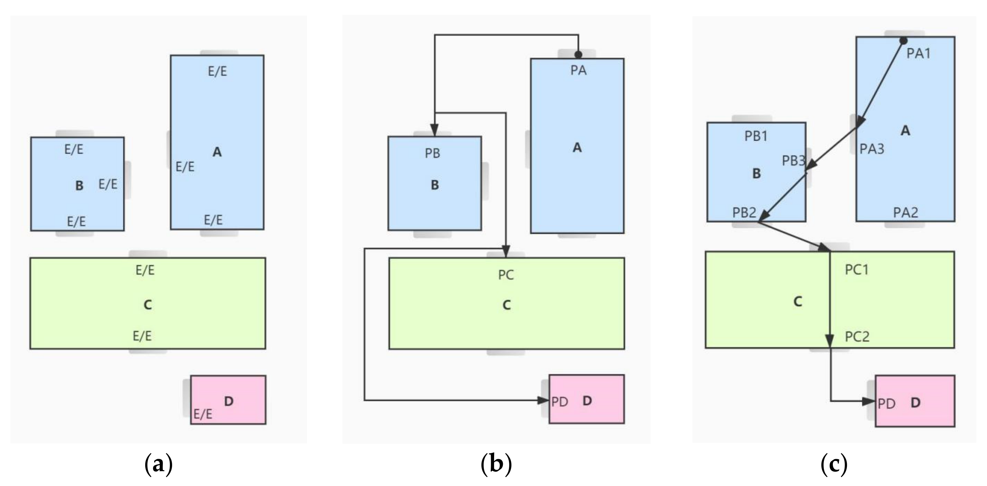
There are three entrances/exits in scenic spots A and B, two entrances/exits in C, and one entrance/exit in D (Figure 1). In traditional tour path planning, scenic spots A, B, C, and toilet D would be mapped as POIs for the scenic road network, PA, PB, PC, and PD, respectively, and the traditional path planning for Route 1 (PA–PB–PC–PD) would be generated (Figure 1b). However, in an actual tour, the entrances and exits of scenic spots A, B, and C have certain connectivity, and Route 2 (PA1–PA3–PB3–PB2PC1–PC2–PD) is a more convenient and efficient tourism route in this situation (Figure 1c). There is a significant difference between Routes 1 and 2. The main reason for this is that the connectivity among the entrances and exits of scenic spots changes the original road network’s topological connection, which, in turn, changes the results of path planning [25].

Moreover, the tourists’ actual demands and preferences for scenic spots to visit is another important factor that should be considered [26]. With the development of Internet technology, social information dissemination has undergone major changes. A large amount of data are generated by using social media data, which expands the breadth and depth of information acquisition [27]. This information is closely related to people’s lives and can more accurately reflect user preferences and satisfaction [28,29].

Therefore, it is more reasonable to recommend tourism routes based on the objective factors of tourists’ travel preferences, travel autonomy, and personalized needs [30,31], combined with the scenic spots’ structural characteristics and the impact of the tourism infrastructure’s location on tourism route planning.

1.2. Main Contributions

In this study, we address how to improve the comfort of outdoor leisure and sightseeing through combining big social data and the spatiotemporal information of the interesting scenic. We analyzed the scenic spots’ structural characteristics and the service facilities’ impact on tourism route planning. Then, we discuss the tourism route planning models and algorithms that take into account multiple entrances and must-visit scenic spots. In this article, we not only consider the structure of the scenic spot, but also the needs and preferences of the tourists. To present the proposed model and algorithms clearly, we consider a very old and well-known garden, Yu Garden, in shanghai, and compare the proposed model and algorithm with the traditional case in both simulations in MATLAB and investigations in the 2bulu app.

The organization of the rest of this paper is as follows: In Section 2, we introduce the models and algorithms and how to create it and how to implement it. In Section 3, we introduce the applications of the model and algorithms in a garden (Yu Garden) considering both the simulated case (simulated data are from Google map and the management of Yu Garden) and investigated case (data are from 2bulu app). Additionally, we compare our proposed methods with traditional methods which regard the scenic spot as a point. In Section 4, we discuss all the simulation results and investigation results. Finally, in Section 5, we conclude this paper and present the limitations and implications of the model and algorithms and give some future research directions.

2. Methods

In this section, we introduce the study area, a local garden (Yu Garden), on which the route planning is verified. Then, we propose a new route plan method combining the Double-Weighted Graph Model (DWGM) and big social data, regarding the scenic spot’s structure and the tourists’ needs and preferences. Additionally, we apply the methods used for Yu Garden for a comparison of simulation data (simulated data from the Google map and the management of Yu Garden) and investigation data (data from the 2bulu app). Finally, we compare our proposed methods with traditional methods regarding the scenic spot as a point.

2.1. Study Area

Yu Garden is an ancient garden located in the Huangpu District of Shanghai, China. It was built in 1559, during the Ming Dynasty, and covers an area of 1.9 ${\mathrm{hm}}^2$. Additionally, it is the only remaining garden of Shanghai’s Old Town. In history, Yu Garden experienced several disasters, and its overall patterns partly changed. However, Yu Garden was listed as Shanghai’s Cultural Heritage in 1959 and a National Cultural Heritage in 1982. Despite experiencing periods of prosperity and decline, damage and restoration, Yu Garden currently retains most of the traditional characteristics of the late Qing Dynasty due to its architectural layout, rockery stacks, corridors, and water system [32].

As a public ancient garden, Yu Garden is one of the key research objects of China’s classical gardens and many classical garden research conferences have been held here. For nearly ten years, its daily number of tourists is larger than 120,000. In holidays, such as Labor Day (from 1 May to 3 May every year) and National Day (from 1 October to 7 October every year), the number is larger than 200,000. Additionally, in China’s traditional holidays, such as Spring Festival and Lantern Festival, the number is larger than 600,000. Leaders from different countries, such as France, Kingdom of Cambodia, Australia, Mongolia, Panama, Hungary, etc., have all visited Yu Garden. Yu Garden has become one of the important scenic spots for recreation and leisure for citizens in Shanghai. Therefore, Yu Garden is an optimal study area to explore the correlation between the tourism route selection and the structure of Chinese classical garden space.

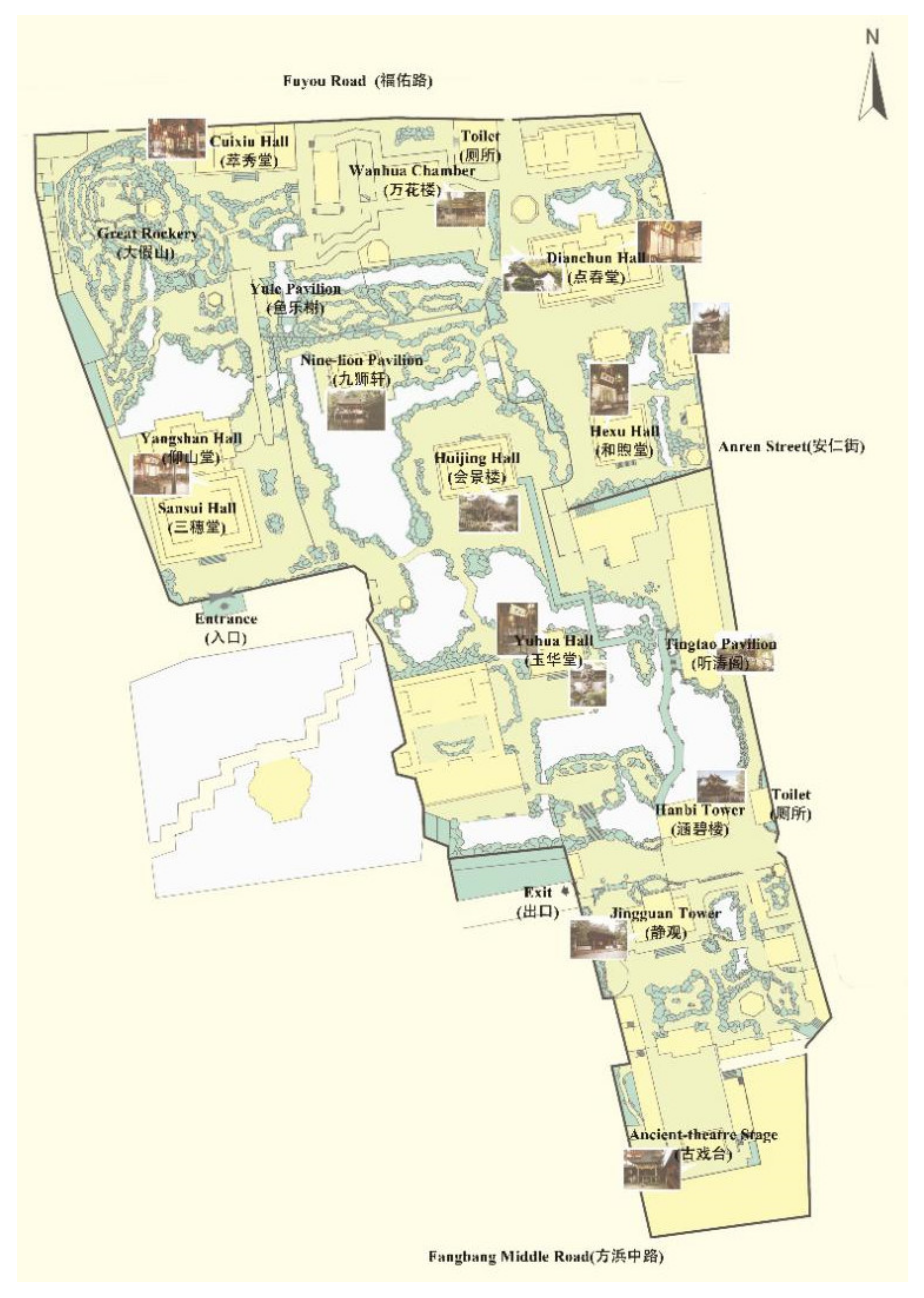
Yu Garden consists of six scenic areas, and each of them has several sub scenics. Therefore, the branch roads inside Yu Garden are intricate (Figure 2). To improve the planning accuracy, we cooperated with the Shanghai Garden Management Center and obtained a detailed map of Yu Garden. Then, we used ArcGIS to digitize Yu Garden’s scenic spots and roads based on the remote sensing image from Google Maps. Thus, the accessible paths and distances between the entrances and exits of each attraction could be calculated (see Section 3 for more details).

2.2. Scenic Spots Selection via Big Social Data

The designing of tourism routes should minimize the cost (money, time, or distance) so as to maximize tourists’ satisfaction [33,34] and allow tourists to reach as many high-popularity scenic spots as possible within a certain period. However, the popularity of each scenic spot indicated by its rating and weight is essential. To identify the popularity of each scenic spot, we downloaded the tourists’ comments from the Dianping website (https://www.dianping.com/ accessed from 1 January to 31 December 2019, using Python). Dianping is the earliest established third-party review platform in China and has formed a highly reputable database to influence public decision-making [35]. Then, we analyzed the word frequency using the Term Frequency (TF) and Inverse Document Frequency (TF-IDF) model [36,37], a formula that aims to define the importance of a keyword or phrase within a document or a web page.

Term frequency, $W_{tf}\left(w,d\right)$, is the frequency of term $w$,

$$W_{tf}\left(w,d\right)=\frac{f_{w,d}}{{{\displaystyle \sum }}_{w^{\prime }\in d}{f^{\prime }}_{w^{\prime },d}}$$

(1)

where $f_{w,d}$ is the raw count of the term $w$ in a document, i.e., the number of times that term $w$ occurs in document $d$.

The inverse document frequency is a measure of how much information the word provides, i.e., if it is common or rare across all documents. It is the inverse fraction of the documents that contain the word (obtained by dividing the total number of documents by the number of documents containing the term, and then taking the logarithm of that quotient):

$$W_{idf}\left(w,D\right)=log\frac{N_d}{\left|N_{w,d}\right|}$$

(2)

where $N_d$ is the total number of documents in the corpus and $N_{w,d}$ is the number of documents where the term $w$ appears. If the term $w$ is not in the corpus, this will lead to a division by zero. It is therefore common to adjust the denominator to $1+\left|N_{w,d}\right|$. Then, the TF-IDF is calculated as,

$$W_{TF-IDF}\left(w\right)=W_{tf}\left(w,d\right)·W_{idf}\left(w,D\right)$$

(3)

According to the TF-IDF model, we defined the popularity gradient as follows: (1) the scenic spots with weights ≥0.8; (2) ≥0.6 and <0.8; (3) ≥ 0.4 and <0.6; and (4) <0.4. The attraction with a weight of less than 0.4 means tourists pay little attention to them; therefore, these attractions were not involved in this study. The scenic popularity of Yu Garden is details in Section 3. The main parameters used in this work are presented in

Table 2. Major parameters used in this work.

Parameters	Definitions
$N$	the total number of scenic spots;
$V_i$	The i-th scenic spot;
$v$	The travel speed of the tourist;
$t_i$	the recommended tour time for $V_i$;
s	The selected starting scenic spot;
${\mathbb{V}}_i$	the set of all entrances and exits for $V_i$;
$N_i$	the number of total entrances and exits for $V_i$, and $|{\mathbb{V}}_i$$|=N_i$;
$E_{i,j}$	the j-th entrance or exit of scenic spot $V_i ;$
|${\mathbb{V}}_i$|	the number of elements in set ${\mathbb{V}}_i$ and $|{\mathbb{V}}_i$$|=N_i$;
$\mathbb{E}$	the set of routes (edges) between entrances and exits;
$N_d$	the total number of documents in the corpus;
$N_{w,d}$	the number of documents where the term $w$ appears;
$W_{tf}\left(w,d\right)$	the frequency of term $w$;
$W_{idf}\left(w,D\right)$	the inverse document frequency of term $w$;
$W_{TF-IDF}\left(w\right)$	the word frequency of term $w$;
$f_e\left(s,V_i\right)$	the weight function for entering the scenic spot (vertex of the graph);
$f_d\left({\mathbb{V}}_i,{\mathbb{V}}_j\right)$	the weight function for departing the scenic spot;
$Dis\left(s,E_{i,j}\right)$	the distance between the starting spot $s$ and $E_{i,j}$ calculated via the Dijkstra algorithm;
$Dis\left(E_{i,k},E_{j,l}\right)$	the distance between the entrance or exit $E_{i,k}$ and $E_{j,l}$ calculated via the Dijkstra algorithm;
$E_{rr}$	the error between the distance which is calculated by the proposed model and the recorded distance through 2bulu app.

.

In addition, the toilet is a special service facility with only one entrance and one way in public gardens, which affects the overall distance planning; however, they are often overlooked in traditional route planning.

2.3. Double-Weighted Graph Model

Based on the traditional scenic graph model (see Section 1 for more details), the double-weighted graph model (DWGM) reflects the influence of the architectural characteristics of the scenic spot on route planning by increasing the dynamic selection of the entrances and exits of the scenic spot. In this work, we introduce the definitions of DWGM for a scenic spot and take the distance weight as an example to provide the weight function of the vertices and edges, as well as the solution of the optimal path.

The scenic spot model in smart tourism is given as

$$\left\{ \begin{array}{llll}{V}_i& =& & \left\{{\mathbb{V}}_i,t_i\right\}\\ {\mathbb{V}}_i& =& \{E_{i,j} | j& =1,2, \cdots ,N_i\}\end{array}\right.$$

(4)

where $V_i$ is the scenic spot, $t_i$ is the recommended tour time for $V_i$, ${\mathbb{V}}_i$ is the set of all entrances and exits for $V_i$, and the j-th entrance or exit of the scenic spot $V_i$ is denoted by $E_{i,j}$. $N_i$ is the number of total entrances and exits for $V_i$, and |${\mathbb{V}}_i$| = $N_i$, where |${\mathbb{V}}_i$| is used to denote the number of elements in set ${\mathbb{V}}_i$. Then, the DWGM for the scenic spot is obtained as

$$\left\{ \begin{array}{c}G=\left\{\mathbb{V}, \mathbb{E}\right\}\\ \mathbb{V}={\displaystyle {\displaystyle \bigcup }_{i=1}^N}{\mathbb{V}}_i \\ \mathbb{E}=\left\{\left(E_{i ,j}, E_{k,l}\right)\right|E_{i ,j}\in {\mathbb{V}}_i, E_{k,l}\in {\mathbb{V}}_k\}\end{array}\right.$$

(5)

where N is the total number of scenic spots. The weight function for the edge is calculated via the Dijkstra algorithm. The Dijkstra algorithm, also called the shortest path algorithm, is usually used to calculate the shortest path algorithm between two given nodes [21]. In the DWGM, there are two weight functions for the edge of a given scenic spot:

• The weight function for entering the scenic spot $V_i$ (vertex of the graph) is denoted by $f_e\left(s,V_i\right)$, and it was given by

  $$f_e\left(s,V_i\right)=\underset{j}{min}\left\{Dis\left(s,E_{i,j}\right)\right\} , j\in \left\{j=1,2, \cdots ,N_i\right\}$$

  (6)
  Here, Dis (s, $E_{i,j}$) is the distance between s and $E_{i,j}$ calculated via the Dijkstra algorithm, and s was selected as the starting spot, which can be the scenic spot and the entrances and exits of the scenic spot.
• The weight function for departing the scenic spot, $f_d\left({\mathbb{V}}_i ,{\mathbb{V}}_j\right)$:

  $$f_d\left({\mathbb{V}}_i ,{\mathbb{V}}_j\right)=\underset{k,l}{min}\left\{Dis\left(E_{i,k},E_{j,l}\right)\right\}, k\in \left\{j=1,2, \cdots ,N_i\right\} , l\in \left\{j=1,2, \cdots ,N_j\right\}$$

  (7)

Suppose that,

• $\mathbb{P}=\left\{V_{i_1}, V_{i_2},\cdots , V_{i_m}\right\}$ is the scenic spot traveled to;
• $\mathbb{Q}=\left\{V_{j_1}, V_{j_2},\cdots , V_{j_n}\right\}$ is the scenic spot passed but not travelled to;
• $ℝ=\left\{V_{l_1}, V_{l_2},\cdots , V_{l_p}\right\}$ is the scenic spot that is neither passed nor travelled to.

Moreover, m + n + p = N. Then, the total travel consumption, including the path length and the travel time, can be formulated as

$$C=F\left(s,e,\mathbb{P},\mathbb{Q}, ℝ \right)$$

(8)

where s is the starting scenic spot (generally the entrance of a park) and e is the end of a tour (generally the exit of a park). Then, according to (1)–(4),

$$F\left(s,e,\mathbb{P},\mathbb{Q}, ℝ \right)={\displaystyle \sum }_{k=1}^m{t}_{i_k}+\frac{1}{v} P,$$

(9)

where $v$ is the speed of the tourist and $P$ is the total travel path. Here, the shorter the path, the shorter the traveling time. The solution for P is the critical travelling salesman problem (also called the travelling salesperson problem, TSP). TSP asks the following question: “Given a list of cities and the distances between each pair of cities, what is the shortest possible route to visit each city and return to the origin city?”. This is an NP-hard problem in combinatorial optimization, which is important in operational research and theoretical computer science:

$$P={\displaystyle \sum }_{k=1}^m{\displaystyle \sum }_{l=1}^n \left(f_e\left(V_{i_k},V_{j_l}\right)+f_d\left(V_{i_k},V_{j_l}\right)\right)$$

(10)

2.4. Construction of DWGM

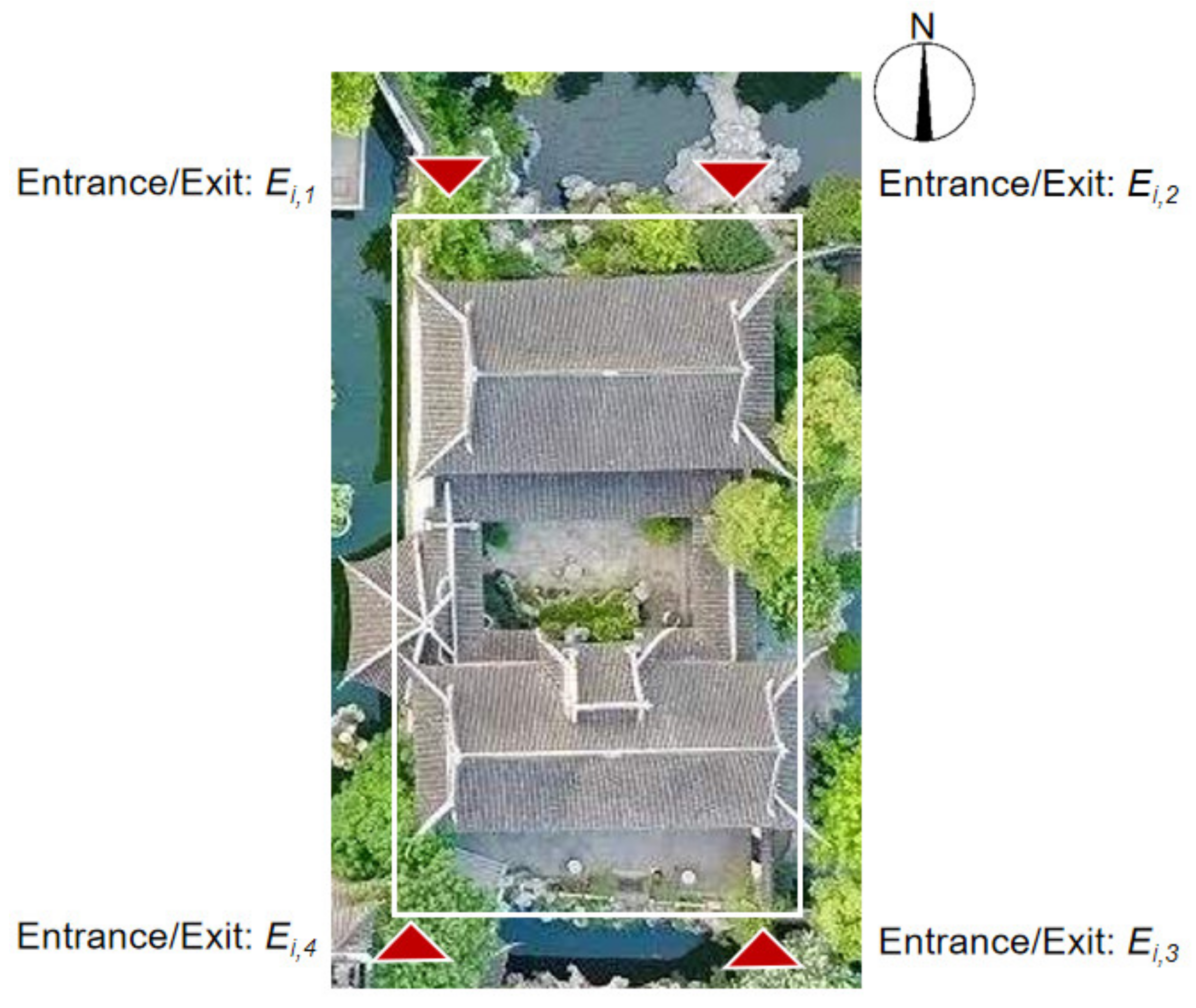
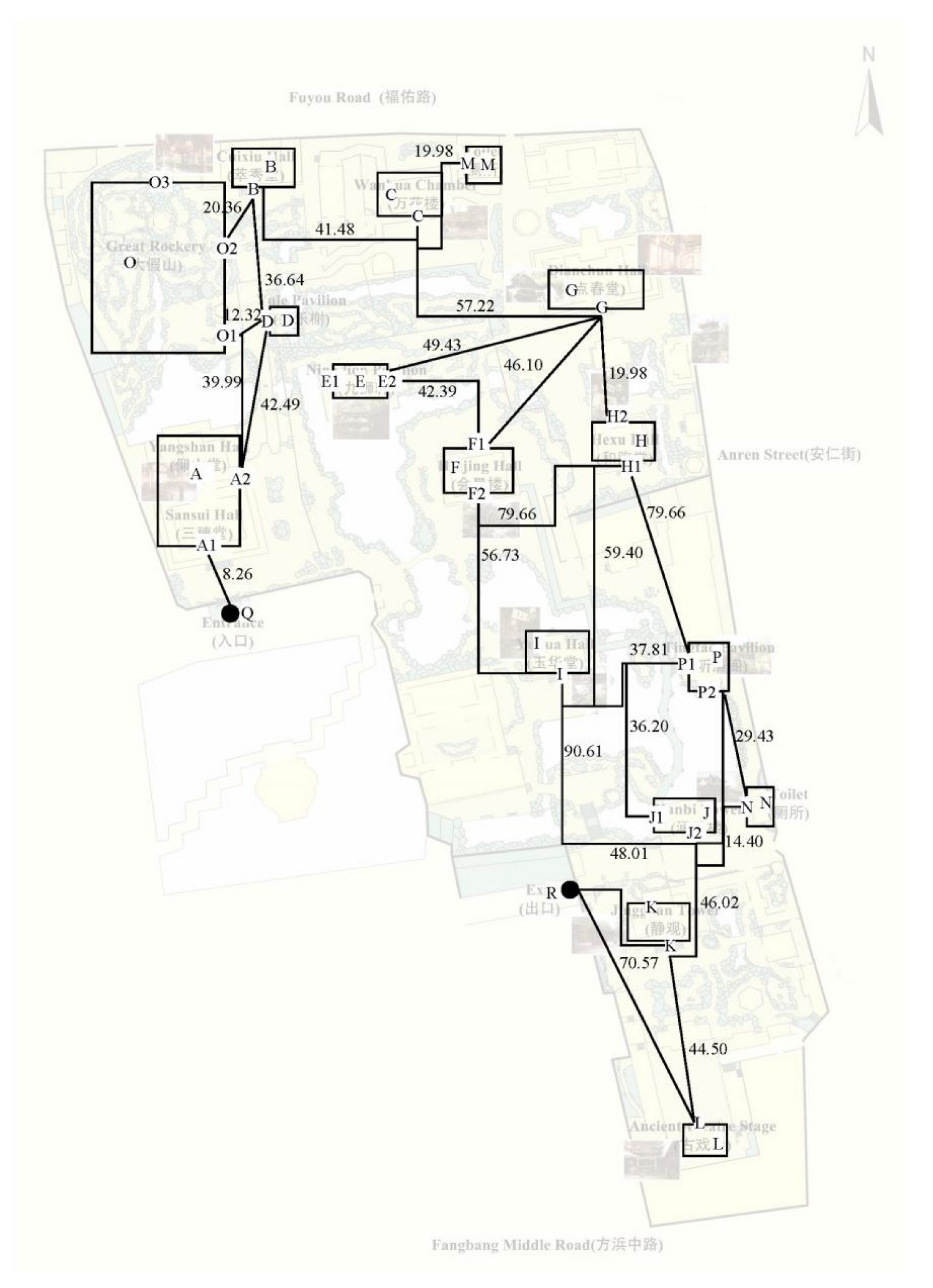
Like other typical classical Chinese gardens, Yu Garden’s spatial layout is characterized by several scenic spots with various entrances and exits and many tourist routes among scenic spots. Based on the DWGM of the scenic spots, we proposed an optimal path planning algorithm. The multiple entrances and exits of the scenic spots are numbered as in Figure 3.

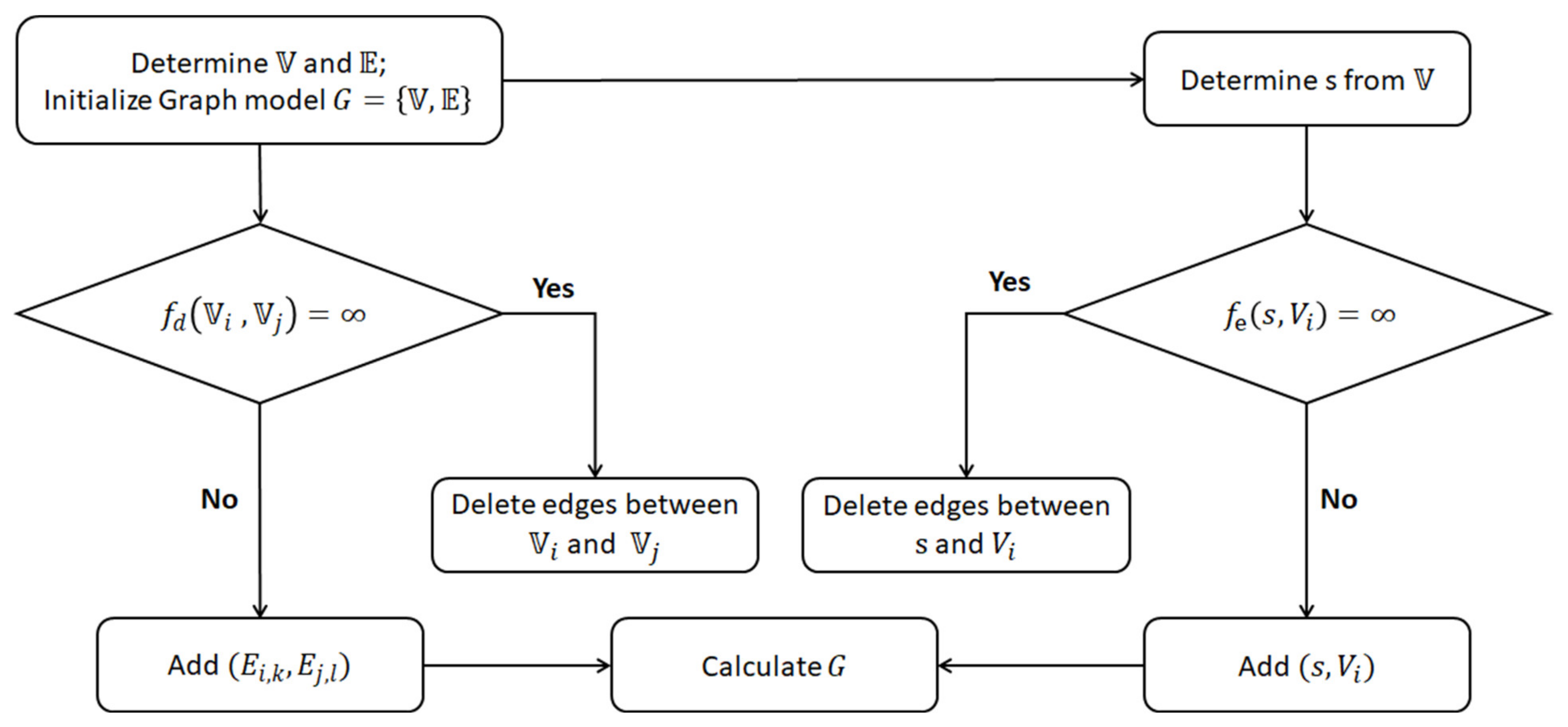
The construction process of the scenic solution graph is as follows (Figure 4):

• Determine the scenic spots and their entrances and exits and construct the vertex set $\mathbb{V}$ according to (4) and (5);
• Construct the edge set $\mathbb{E}$ according to (4) and (5);
• Calculate all weight functions for all edges according to (6) and (7);
• Delete the edges that are not directly related (the edge weight is ∞) and construct the double-weighted graph model (DWGM);
• Select the starting (s) and ending (e) positions of the tour;
• Based on (8)–(10), solve the total consumption of the tour.

2.5. Investigations Using the 2bulu App

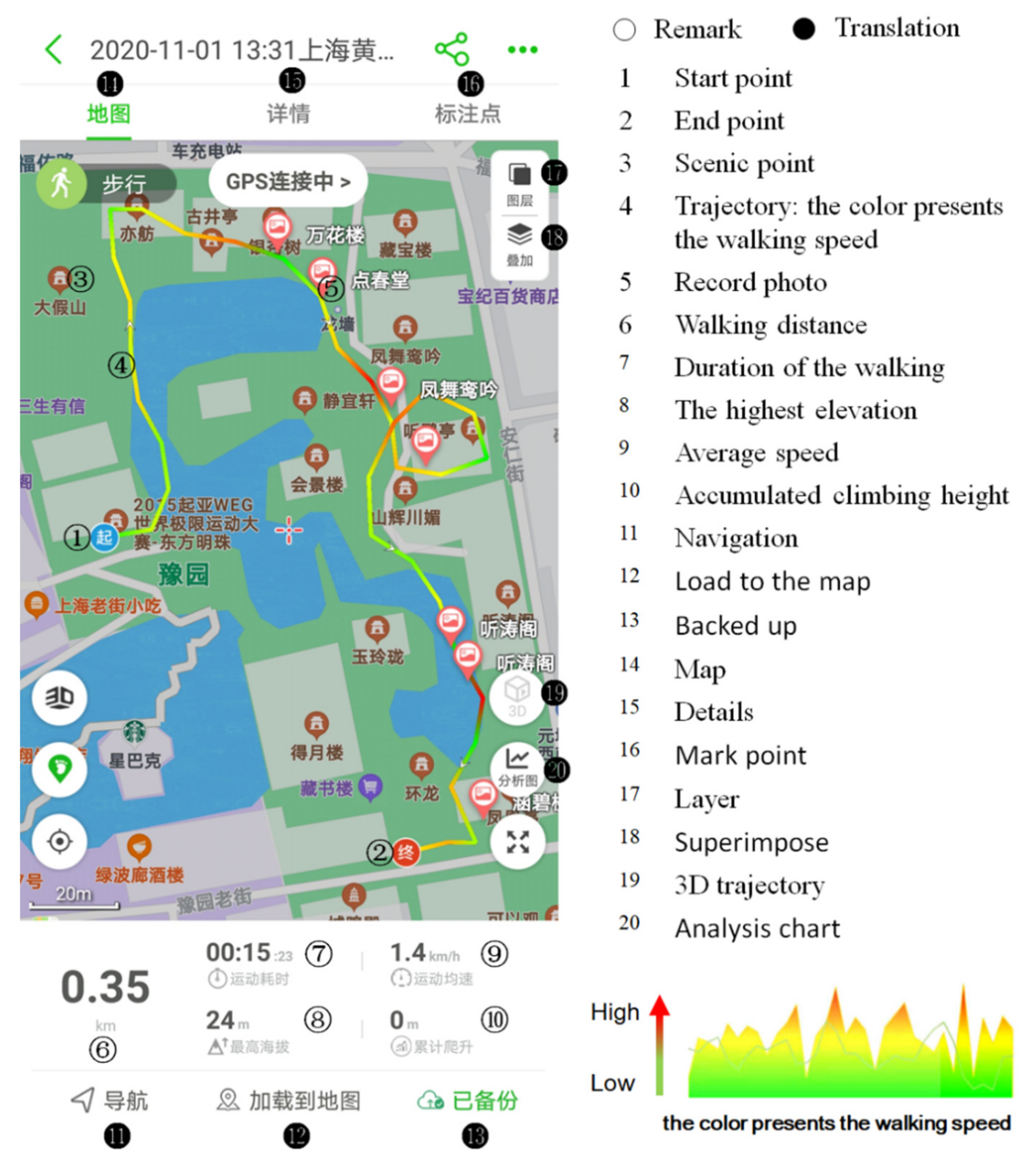
In the investigation, we used the 2bulu app (Figure 5) to record the three-dimensional trajectory of the volunteers. The 2bulu app is a Chinese professional outdoor mobile app for assisting outdoor fitness with accurate GPS positioning function, developed by Shenzhen 2bulu Information Technology Co. LTD., Shenzhen, China, launched on both iOS and Android app stores. It can be download from the official website: http://www.2bulu.com/ (accessed on 25 June 2021). It is also designed to provide the professional outdoor maps and navigation functions, as well as precise outdoor track routes. It is widely used in daily travel, route planning, motion record analysis, distance measurement, and altitude measurements, etc.

Figure 5 presents a screenshot of the 2bulu app. In Figure 5, it can be seen that the 2bulu app is able to record the visit trajectory, the travel duration, the speed, the total distance, the elevation, etc.

In the investigation, ten participants were divided into five groups, and each group was given a route plan. Two participants in each group were required to walk together through Yu Garden along the planned paths. The only difference between the two participants in one group is that one visitor should use a toilet at a time while the other should not. Whilst walking, they had to make sure the 2bulu app was working in the record mode for data collection. The participants also recorded the pairwise walking time at each scenic spot to calculate the average stay at each, combining this with data stored in the 2bulu app. We calculated the error based on the simulated and recorded distances to make a comparison between the traditional and the new algorithms. The error calculation method is given as:

$$E_{rr}=\frac{\left|r\ast 1000-c\right|}{r\ast 1000}\ast 100\%$$

(11)

where $r$ is the recorded distance and $c$ is the simulated distance obtained through the 2bulu app.

3. Results

3.1. The Scenic Spots Popularity Based on TF-IDF Model and Big Social Data

After cleaning the invalid information, such as tourist comments not related to the scenic area, 6199 effective reviews were finally obtained. According to the word frequency analysis, the TF-IDF model defined in (1)–(3), scenic spots’ popularity was determined by their weight: the scenic spot with a $\mathrm{Weight}\ge 0.8$ is the Great Rockery; the scenic spots with weights: $0.6 \le \mathrm{Weight}<0.8$ (

Table 3. The weight and ranking of the scenic spots of Yu Garden.

Weight	Scenic Name
Weight ≥ 0.8	Great Rockery (假山)
0.6 ≥ Weight < 0.8	Dianchun Hall (点春堂), Sansui Hall (三穗堂), Ancient Theatre Stage (古戏台), Jing Pavilion (静观), Hanbi Tower (涵碧楼), Tingtao Pavilion (听涛阁), Wanhua Building (万花楼)
0.4 ≤ Weight < 0.6	Yuhua Hall (玉华堂), Huijing Building (会景楼), Cuixiu Hall (萃秀堂), Hexu Hall (和煦堂), Jiushi Pavilion (九狮轩), Yule Pavilion (鱼乐榭),
Weight < 0.4	Deyue Chamber (得月楼), Depository of Books and Paintings (藏书楼), Relic Hall (藏宝楼), Master Lao Hall (老君殿), Exhibit Hall (展览厅), Keyl Hall (可以观), Huanyun Hall (还云楼), Songcui Pavilion (耸翠亭), Yanqing Tower (延清楼), Kuailou Pavilion (快楼)

) are Dianchun Hall, Sansui Hall, the Ancient Theatre Stage, Jing Pavilion, Hanbi Tower, Tingtao Pavilion, and Wanhua Building; the scenic spots with weights: $0.4 \le \mathrm{Weight}<0.6$ are Yuhua Hall, Huijing Building, Cuixiu Hall, Hexu Hall, Jiushi Pavilion, and Yule Pavilion. These scenic spots are showed to have high cultural and aesthetic value and are distributed evenly and cover almost all of the garden’s area. The ones that with weights smaller than 0.4 (as presented in Table 3) are not well-recommended by big social data. However, the tourists could still visit them according to their own plan.

According to the analysis results of the scenic spots’ weights and rankings, 14 representative scenic spots whose weights are greater than 0.4 and all their entrances and exits, as well as two toilets, have been chosen as the components of planning routes in this study (

Table 4. The marks and description of the chosen scenic spots of Yu Garden.

Mark	Scenic Spots	Scenic Spot Description
A	Sansui Hall	Nine meters in height, Sansui Hall is one of the Garden’s main building as was re-established 25 years ago since the ruling of Emperor Qianlong (1760).
B	Cuixiu Hall	Built in the 25th year into Emperor Qianlong’s rule (1760) and deeply hidden in the north of the Great Rockery.
C	Wanhua Building	It was a temple of the gods and was built in the Ming Dynasty (1368–1644). The existing building was built in the time of Emperor Daoguang (1821–1851).
D	Yule Pavilion	Yule Pavilion is a small Chinese garden with an attractive landscape, its flowers, pavilions, trees, and other elements can be dating back 300 years.
E	Jiushi Pavilion	It is an open architecture, facing a large pool and with a platform.
F	Huijing Building	As the main building, Huijing Building is located at the center of Yu Garden, which is dominated by a water landscape.
G	Dianchun Hall	Dianchun Hall used to be the command department of Shanghai Small-Sword Society, and now is a hall displaying the cultural relics of the organization.
H	Hexu Hall	Hexu Hall faces the lakeside rockeries and is surrounded by windows and has a set of furniture over 200 years old.
I	Yuhua Hall	It is the study room of the owner of Yu Garden, in which the furniture is of the Ming Dynasty with superb artistic structures and elegant taste.
J	Hanbi Tower	The material of the building is top grade nanmu wood of Myanmar, which is a superior wood product and rare in China.
K	Jing Pavilion	It is an important architecture for visitors to have a thorough look at the opposite rockeries quietly.
L	Ancient Theatre Stage	It is called the first stage of the southeast with carved and painted beams.
M	Toilet	At the north of the garden.
N	Toilet	At the south of the garden.
O	Great Rockery	It was designed and built by Zhang Nanyang, a famous rocky piling specialist living in the Ming Dynasty.
P	Tingtao Pavilion	The location of Tingtao Pavilion is near Huangpu River. Located at the north of the building, it is a famous exhibition hall.
Q	Entrance	At the west end of the garden.
R	Exit	At the south end of the garden.

).

3.2. Tourism Routes Regeneration Based on the DWGM

Based on the DWGM, Dijkstra and TSP algorithms for finding the shortest path, five optimal tourism routes in Yu Garden were regenerated according to the scenic spots’ weights and rankings, as well as the distance analysis among them (as presented in Figure 6 and

Table 5. Results of the tourist route planning of the experimental area.

Plan	Tourist Routes	Distance (m)
1	$\mathrm{Q}-{\mathrm{A}}_1$$-{\mathrm{A}}_2$$-\mathrm{D}-O_1$$-O_3$$-\mathrm{B}-\mathrm{C}-\mathrm{G}-{\mathrm{E}}_2$$-F_1$$-{\mathrm{F}}_2$$-H_1$$-\mathrm{I}-P_1$$-{\mathrm{P}}_2$$-{\mathrm{J}}_2$-K-L-R	656.84
2	$\mathrm{Q}-{\mathrm{A}}_1$$-{\mathrm{A}}_2$$-\mathrm{D}-O_1$$-O_3$$-\mathrm{B}-\mathrm{C}-\mathrm{M}-\mathrm{G}-{\mathrm{E}}_2$$-F_1$$-{\mathrm{F}}_2$$-H_1$$-\mathrm{I}-P_1$$-{\mathrm{P}}_2$$-{\mathrm{J}}_2$-K-L-R	686.91
3	$\mathrm{Q}-{\mathrm{A}}_1$$-{\mathrm{A}}_2$$-O_1$$-O_2$$-\mathrm{C}-\mathrm{G}-P_1$$-{\mathrm{P}}_2$$-{\mathrm{J}}_2$-K-L-R	463.04
4	$\mathrm{Q}-{\mathrm{A}}_1$$-{\mathrm{A}}_2$$-O_1$$-O_2$$-\mathrm{C}-\mathrm{M}-\mathrm{G}-P_1$$-{\mathrm{P}}_2$$-{\mathrm{J}}_2$-K-L-R	493.11
5	$\mathrm{Q}-{\mathrm{A}}_1$$-{\mathrm{A}}_2$$-O_1$$-O_2$$-\mathrm{C}-\mathrm{G}-P_1$$-{\mathrm{P}}_2$$-\mathrm{N}-{\mathrm{J}}_2$-K-L-R	464.05

).

In this study, for different target tourists, two tourism routes with or without toilets were proposed. The first one was planned for ordinary tourists who want to see more attractions, including 14 recommended scenic spots (Great Rockery, Dianchun Hall, Sansui Hall, the Ancient Theatre Stage, Jing Pavilion, Hanbi Tower, Tingtao Pavilion, Wanhua Building, Yuhua Hall, Huijing Building, Cuixiu Hall, Hexu Hall, Jiushi Pavilion, and Yule Pavilion). These routes considered both the popularity of the attractions and tourists’ needs, representing the best choice, and providing a rich sensory experience. Another route for tourists who have a limitation with regard to visiting time and energy includes eight of the most famous attractions (Great Rockery, Dianchun Hall, Sansui Hall, Ancient-theatre Stage, Jing Pavilion, Hanbi Tower, Tingtao Pavilion, Wanhua Building), whose weights and rantings are ≥ 0.6. These routes are also suitable for older tourists to appreciate the attractions’ charms in the shortest time.

Route 1: Q-${\mathrm{A}}_1$-${\mathrm{A}}_2$-D-$O_1$-$O_3$-B-C-G-${\mathrm{E}}_2$-$F_1$-${\mathrm{F}}_2$-$H_1$-I-$P_1$-${\mathrm{P}}_2$-${\mathrm{J}}_2$-K-L-R. The total length of the route is 656.84 m, and there is no toilet available over the whole journey.

Route 2: Q-${\mathrm{A}}_1$-${\mathrm{A}}_2$-D-$O_1$-$O_3$-B-C-M-G-${\mathrm{E}}_2$-$F_1$-${\mathrm{F}}_2$-$H_1$-I-$P_1$-${\mathrm{P}}_2$-${\mathrm{J}}_2$-K-L-R. The total length of the route is 686.91 m, including a toilet on the tour route. This plan considers the route distance and the duration of the tour. Toilet M was included because it is located about halfway through the tour.

Route 3: Q-${\mathrm{A}}_1$-${\mathrm{A}}_2$-$O_1$-$O_2$-C-G-$P_1$-${\mathrm{P}}_2$-${\mathrm{J}}_2$-K-L-R. The total length of the route is 463.04 m, excluding toilets throughout the journey.

Route 4: Q-${\mathrm{A}}_1$-${\mathrm{A}}_2$-$O_1$-$O_2$-C-M-G-$P_1$-${\mathrm{P}}_2$-${\mathrm{J}}_2$-K-L-R. The total length of the route is 493.11 m, and the route includes one toilet. Considering the planned route distance and the duration of the tour, toilet M was selected at a location about halfway through the tour.

Route 5: Q-${\mathrm{A}}_1$-${\mathrm{A}}_2$-$O_1$-$O_2$-C-G-$P_1$-${\mathrm{P}}_2$-N-${\mathrm{J}}_2$-K-L-R. The route has a total length of 464.05 m and has one toilet. Due to the small number of tourist attractions, visitors can choose toilet N located at the end of the tour.

3.3. Investigation Results Based on the 2bulu App

The investigation results are presented in

Table 6. Results of experiments of tourists wandering along the planning routes.

Group	Plan	Planning Route	Sim-Dis 1 (m)	Dur. 2 (min)	W.C.	Rec-Dis 3 (km)	Err-Dis 4 (%)
1	1-1	Q-${\mathrm{A}}_1$-${\mathrm{A}}_2$-D-${\mathrm{O}}_1$-${\mathrm{O}}_3$-B-C-G-${\mathrm{E}}_2$-${\mathrm{F}}_1$-${\mathrm{F}}_2$-${\mathrm{H}}_1$-I-${\mathrm{P}}_1$-${\mathrm{P}}_2$-${\mathrm{J}}_2$-K-L-R	657	102.6	No	0.76	13.16
	1-2	Q-${\mathrm{A}}_1$-${\mathrm{A}}_2$-D-${\mathrm{O}}_1$-${\mathrm{O}}_3$-B-C-G-${\mathrm{E}}_2$-${\mathrm{F}}_1$-${\mathrm{F}}_2$-${\mathrm{H}}_1$-I-${\mathrm{P}}_1$-${\mathrm{P}}_2$-N-${\mathrm{J}}_2$-K-L-R	687	95.5	N	0.78	11.54
2	2-1	Q-${\mathrm{A}}_1$-${\mathrm{A}}_2$-${\mathrm{O}}_1$-${\mathrm{O}}_2$-C-G-${\mathrm{P}}_1$-${\mathrm{P}}_2$-${\mathrm{J}}_2$-K-L-R	463	57.3	No	0.46	0.65
	2-2	Q-${\mathrm{A}}_1$-${\mathrm{A}}_2$-${\mathrm{O}}_1$-${\mathrm{O}}_2$-C-M-G-${\mathrm{P}}_1$-${\mathrm{P}}_2$-${\mathrm{J}}_2$-K-L-R	493	58.8	M	0.54	9.26
3	3-1	Q-A-D-O-B-C-G-E-F-H-I-P-J-K-L-R	516	106.3	No	0.68	24.12
	3-2	Q-A-D-O-B-C-M-G-E-F-H-I-P-J-K-L-R	534	107.2	M	0.67	20.30
4	4-1	Q-A-O-C-G-P-J-K-L-R	405	108.0	No	0.61	33.61
	4-2	Q-A-O-C-G-P-N-J-K-L-R	425	102.0	N	0.62	31.45

¹ Sim-Dis: the calculated distance through the proposed model. ² Dur.: the duration spent in the scenic spot. ³ Rec-Dis: the recorded distance through the 2bulu app. ⁴ Err-Dis: the distance error of the calculated distance over the record distance through Formula (8) through the proposed model.

and

Table 7. Average stay at each scenic spot.

Mark	Scenic Spot	Average Stay on Each Scenic Spot (min)
A	Sansui Hall	2.83
B	Cuixiu Hall	2.27
C	Wanhua Building	2.64
D	Yule Pavilion	2.31
E	Jiushi Pavilion	3.00
F	Huijing Building	3.75
G	Dianchun Hall	3.98
H	Hexu Hall	2.59
I	Yuhua Hall	4.88
J	Hanbi Tower	2.15
K	Jing Pavilion	1.84
L	Ancient Theatre Stage	4.78
M	Toilet	3.45
N	Toilet	3.00
O	Great Rockery	4.50
P	Tingtao Pavilion	3.41
Q	Entrance	1.17
R	Exit	0.48

.

Table 6 presents the investigation data using the same planned route that was calculated through simulation. The investigation data including the calculated distance through the proposed model (Sim-Dis), the duration spent in the scenic spot (Dur.), use of the toilet or not (W.C.), the recorded distance through the 2bulu app (Rec-Dis), and the distance error of the calculated distance over the recorded distance through formula (8) (Err-Dis) through the proposed model.

Table 7 presents the average stay at each scenic spot. The average stays are recorded through the 2bulu app. From Table 7, we could find the popularity of each scenic spot according to the stay duration. Compared to Table 3, the popularity of the scenic spot almost coincides with the dib social data from the Dianping website.

4. Discussion

4.1. Discussion about the Simulation Results

Our results showed that the new algorithm concerning the architectural characteristics of scenic spots has a better performance regarding accuracy than traditional ones considering scenic spots, such as PoIs, and brings higher satisfaction to the tourists. Existing sightseeing route planning only adopts the narrow notion of POIs as many spots lack architectural dimensions. Therefore, the planned route proposes to use buildings, small squares and historical landscapes as single-entry points. The impacts of the structural characteristics of the attractions’ entrances and exits on the planned routes are ignored. When it comes to a small-scale landscape area, such ignorance will increase mistakes in route planning for tourists.

Combining scenic spots’ attractiveness and diversified demand of tour time, we recommend four detailed routes for tourists that contain the exit and entrance of each scenic spot, and use $P\left(d,t\right)$ as a reference for different type of routes, where d is the distance of the route and t is the tour time of the route.

• ${\mathrm{P}}_1$(657, 102.6) = Q-${\mathrm{A}}_1$-${\mathrm{A}}_2$-D-${\mathrm{O}}_1$-${\mathrm{O}}_3$-B-C-G-${\mathrm{E}}_2$-${\mathrm{F}}_1$-${\mathrm{F}}_2$-${\mathrm{H}}_1$-I-${\mathrm{P}}_1$-${\mathrm{P}}_2$-${\mathrm{J}}_2$-K-L-R
• ${\mathrm{P}}_2$(687, 95.5) = Q-${\mathrm{A}}_1$-${\mathrm{A}}_2$-D-${\mathrm{O}}_1$-${\mathrm{O}}_3$-B-C-G-${\mathrm{E}}_2$-${\mathrm{F}}_1$-${\mathrm{F}}_2$-${\mathrm{H}}_1$-I-${\mathrm{P}}_1$-${\mathrm{P}}_2$-N-${\mathrm{J}}_2$-K-L-R
• ${\mathrm{P}}_3$(463, 57.3) = Q-${\mathrm{A}}_1$-${\mathrm{A}}_2$-${\mathrm{O}}_1$-${\mathrm{O}}_2$-C-G-${\mathrm{P}}_1$-${\mathrm{P}}_2$-${\mathrm{J}}_2$-K-L-R
• ${\mathrm{P}}_4$(493, 58.8) = Q-${\mathrm{A}}_1$-${\mathrm{A}}_2$-${\mathrm{O}}_1$-${\mathrm{O}}_2$-C-M-G-${\mathrm{P}}_1$-${\mathrm{P}}_2$-${\mathrm{J}}_2$-K-L-R

Concerning many choices of tourist routes, on the one hand, tourists can decide to visit as many attractions as possible in a relatively short time. On the other hand, tourists will be highly flexible in their route selection, especially when considering individual interests and needs among different tourists.

The route plan made by the new algorithm has three advantages. First, it includes the exact distance and time duration, which can help tourists choose a route that fits around their schedule. Second, it recommends scenic spots for tourists based on information from the social network provided by someone who has been there. Third, the route plan with each spot’s entrance and exit of can offer a reasonable, smooth and complete sightseeing route than traditional plans.

4.2. Discussion about the Investigation Results

In Table 6, one can see that the visiting duration of the whole trip varied from 45.9 to 108.0 min and the recorded visiting distance in the 2bulu app ranged from 0.35 to 0.76 km. The visiting distance is relevant to the number of visits to scenic spots. The larger the number of visits to scenic spots, the longer the visiting distance. The visiting durations are not fully dependent on the number of visits to scenic spots. This is because the visiting not only include the walking duration but also include the stay duration in each scenic. Additionally, the stay duration is randomly according to the needs of the tourists.

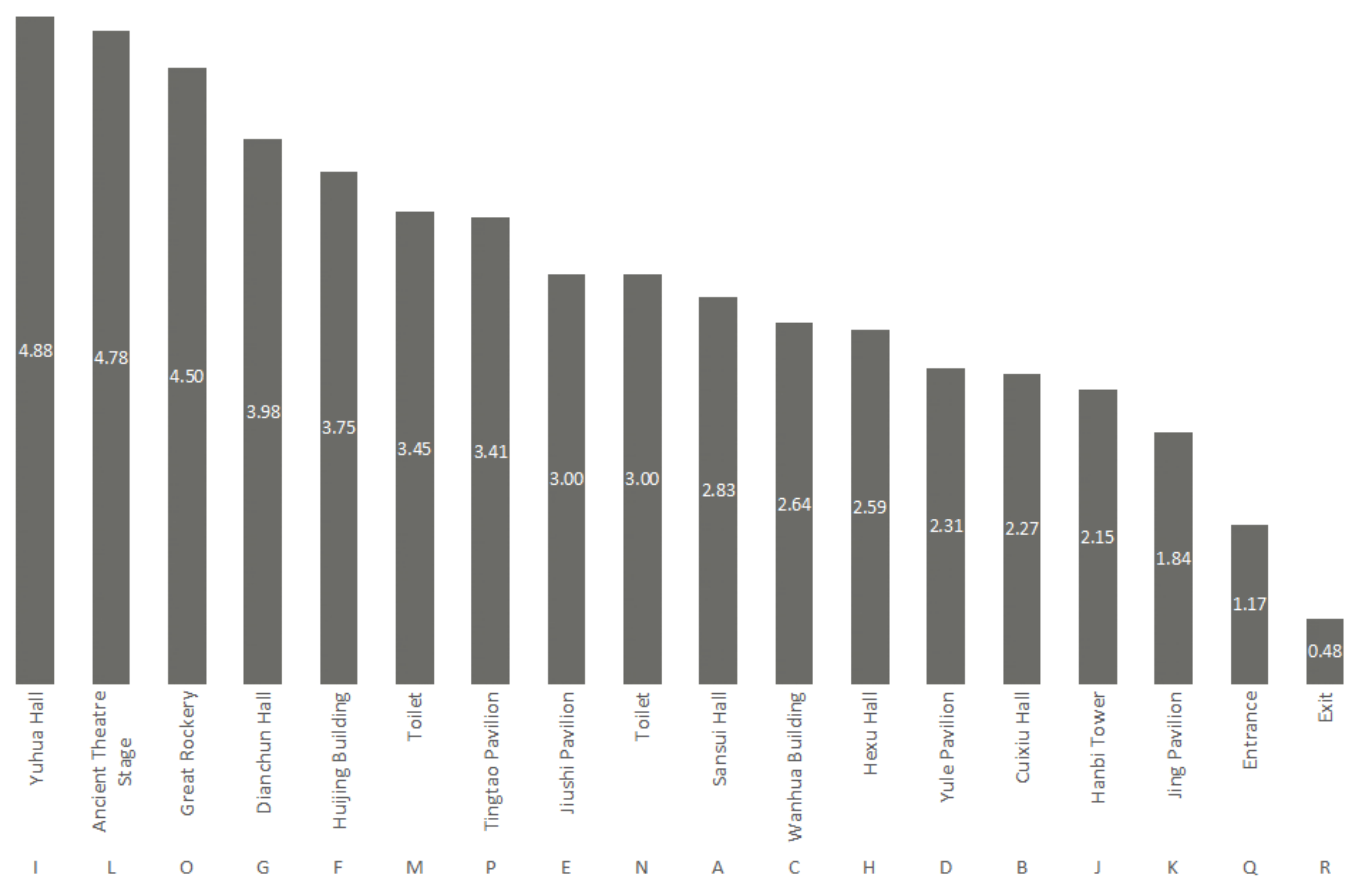
Furthermore, according to the average stay time of participants, the top four duration scenic spots indicated higher weight rankings, except for Yuhua Hall (Table 7 and Figure 7). As Yuhua Hall had a platform close to the lake with lots of resting facilities, it was also located at the end of the tour route, where tourists usually want to relax. Great Rockery, Ancient Theatre Stage, and Dianchun Hall ranked very highly in terms of participants’ stay duration and preference, which reflects the accordance between the social network and tourists’ willingness to stay on spots in reality. Additionally, the main exit and entrance ranked very low due to being less interesting than other scenic spots.

4.3. Comparison between Investigation and Simulation

In Table 5 and Table 6, it can be seen that the visiting distance is a bit longer than the simulated distance in the same route planning. This is because the simulation does not consider the rugged level of the road. There are many stone paved roads and rockeries in Yu Garden which cause more difficulty than in simulations in which all the roads are considered as smooth ones.

It also can be seen in Table 6 that the error of distance in each plan was under 34% and half of all errors were under 15%. From the errors in Group 1 and Group 3, wherein different participants visited the same scenic spots, we noticed that the new algorithm reduced the errors of distance by half. Similar results were shown in Group 2 and Group 4: the errors in Group 2 were under 10%, far fewer than the errors of about 30% in Group 4. Comparing errors in each group, no significant difference was found between the use-toilet plan and no-use-toilet plan except for Group 2, which means using the toilet had little impact on the simulation.

However, dynamic information, such as the real-time passenger flow and dynamic traffic conditions of scenic spots, was not considered in this study. In a further study, we will integrate the characteristics of scenic spots and tourists’ preferences with multi-source data, such as social networks and social computing models, and consider establishing a comprehensive weight calculation model.

4.4. Discussion for Academic

In this research, a new model, which considers not only the spatiotemporal details of the scenery but also the tourists’ preference, is applied. The DWG model is an enhanced graph model and is double-weighted. It enhances the traditional graph model in route planning which does not fully consider the details of the scenic spots and it enriches the research field of tourism route planning.

4.5. Discussion for Management

With the widespread use of social networks, tourists provide much information online which is very important for the management of tourism spots. It not only contains the characteristics of the tourists, but also contains their preferences. Then, the scenic managers are able to obtain what should be focused on through analyzing this information. For example, via this research, scenic management could provide different visit plans for different tourists. This could help enhance the efficiency of their marketing. It would be more meaningful if these managers consider the voice of their visitors.

5. Conclusions

In this study, we used social network data to capture tourists’ preferences combined with the attractions’ popularity to filter scenic spots. This was achieved by using the open-source spatial data and the TSP algorithm solution regarding the spatial structure of multiple entrances and exits of the scenic spots and calculating five tourist routes according to different tour requirements. Through investigated data, we compared the calculated value via the double-weighted graph model (DWGM) with the recorded value, which were obtained from the 2bulu app. The comparison results show that the planned routes through the DWGM are close to the actual value. Additionally, the proposed method has a better performance with regard to error analysis in terms of accuracy.

These research results are able to provide visitors with more precise route guidance and help to construct better scenic spot services. In the future, the proposed DWGM model will be used in tourism webpages and scenic management in combination with the tourism data provided by them. This will provide more accurate planning for people’s leisure travel life and bring better experiences. It is worth noting that one of the cores of this research is the data source. Most of the used data could be obtained through open map software such as Baidu—www.map.baidu.com (accessed on 25 June 2021) and Gaode: www.amap.com (accessed on 25 June 2021). However, it may bring limitations to the research implementations if the research requires highly accurate planning and all the details of the study area.

References

- De la Calle-Vaquero, M.; García-Hernández, M.; de Miguel, S.M. Urban Planning Regulations for Tourism in the Context of Overtourism. Applications in Historic Centres. Sustainability 2021, 13, 70. [Google Scholar] [CrossRef]
- Khamsing, N.; Chindaprasert, K.; Pitakaso, R.; Sirirak, W.; Theeraviriya, C. Modified ALNS Algorithm for a Processing Application of Family Tourist Route Planning: A Case Study of Buriram in Thailand. Computation 2021, 9, 23. [Google Scholar] [CrossRef]
- Du, J.; Zhou, J.; Li, X.; Li, L.; Guo, A. Integrated self-driving travel scheme planning. Int. J. Prod. Econ. 2021, 232, 107963. [Google Scholar] [CrossRef]
- Mei, Y. Study on the application and improvement of ant colony algorithm in terminal tour route planning under Android platform. J. Intell. Fuzzy Syst. 2018, 35, 2761–2768. [Google Scholar] [CrossRef]
- Zhou, X.; Sun, B.; Li, S.; Liu, S. Tour Route Planning Algorithm Based on Precise Interested Tourist Sight Data Mining. IEEE Access 2020, 8, 153134–153168. [Google Scholar] [CrossRef]
- Cuomo, M.T.; Tortora, D.; Foroudi, P.; Giordano, A.; Festa, G.; Metallo, G. Digital transformation and tourist experience co-design: Big social data for planning cultural tourism. Technol. Forecast. Soc. Change 2021, 162, 120345. [Google Scholar] [CrossRef]
- Zhou, X.; Zhan, Y.H.; Feng, G.H.; Zhang, D.; Li, S.M. Individualized Tour Route Plan Algorithm Based on Tourist Sight Spatial Interest Field. ISPRS Int. J. Geo Inf. 2019, 8, 192. [Google Scholar] [CrossRef] [Green Version]
- Barrena, E.; Laporte, G.; Ortega, F.A.; Pozo, M.A. Planning ecotourism routes in nature parks. In Trends in Differential Equations and Applications; Springer: Cham, Switzerland, 2016; pp. 189–202. [Google Scholar]
- Zhou, X.; Su, M.Z.; Liu, Z.; Hu, Y.; Sun, B.; Feng, G.H. Smart Tour Route Planning Algorithm Based on Naïve Bayes Interest Data Mining Machine Learning. ISPRS Int. J. Geo Inf. 2020, 9, 112. [Google Scholar] [CrossRef] [Green Version]
- Lu, Y.; Shahabi, C. An arc orienteering algorithm to find the most scenic path on a large-scale road network. In Proceedings of the 23rd SIGSPATIAL International Conference on Advances in Geographic Information Systems, Seattle, WA, USA, 3–6 November 2015; pp. 1–10. [Google Scholar]
- Aljubayrin, S.; Qi, J.; Jensen, C.S.; Zhang, R.; He, Z.; Wen, Z. The safest path via safe zones. In Proceedings of the 31st International Conference on Data Engineering (ICDE), Seoul, Korea, 13–17 April 2015; pp. 531–542. [Google Scholar]
- Su, J.G.; Winters, M.; Nunes, M.; Brauer, M. Designing a route planner to facilitate and promote cycling in Metro Vancouver, Canada. Transp. Res. Part. A Policy Pract. 2010, 44, 495–505. [Google Scholar] [CrossRef]
- Angskun, T.; Angskun, J. A travel planning optimization under energy and time constraints. In Proceedings of the 2009 International Conference on Information and Multimedia Technology, Jeju, Korea, 16–18 December 2009; pp. 131–134. [Google Scholar]
- Xiao, Z.; Yuan, Y.F.; Li, H.S. City Tour Route Planning Model Based on Improved Floyd Algorithm. In Proceedings of the 2017 International Conference on Mathematics, Modelling and Simulation Technologies and Applications (MMSTA 2017), Xiamen, China, 24–25 December 2017; pp. 13–18. [Google Scholar]
- Gavalas, D.; Kasapakis, V.; Konstantopoulos, C.; Pantziou, G.; Vathis, N. Scenic route planning for tourists. Pers. Ubiquitous Comput. 2017, 21, 137–155. [Google Scholar] [CrossRef]
- Cenamor, I.; de la Rosa, T.; Núñez, S.; Borrajo, D. Planning for tourism routes using social networks. Expert Syst. Appl. 2017, 69, 1–9. [Google Scholar] [CrossRef]
- Teng, C.; Cao, W. Study on filtering sight spots and getting the optional travel route. J. Geo Inf. Sci. 2010, 12, 668–673. [Google Scholar]
- Xu, F.; Du, J. Main Algorithms Study and Implementation of Tourist Spot Navigation System. In Proceedings of the International Conference on Computational Intelligence and Software Engineering, Wuhan, China, 11–13 December 2009. [Google Scholar]
- Kaufman, D.; Smith, R. Fastest paths in time-dependent networks for intelligent vehicle-highway systems application. IVHS J. 1993, 1, 1–11. [Google Scholar] [CrossRef]
- Colorni, A.; Dorigo, M.; Maniezzo, V. Distributed optimization by ant colonies. In Proceedings of the European Conference on Artificial Life, Paris, France, 11–13 December 1991; pp. 134–142. [Google Scholar]
- Li, T.; Zhang, J.; Wang, S.; Lv, Z. Research on route planning based on quantum-behaved particle swam optimization algorithm. In Proceedings of the 2014 IEEE Chinese Guidance, Navigation and Control Conference (CGNCC), Yantai, China, 8–10 August 2014; pp. 335–339. [Google Scholar]
- Hopfield, J.J.; Tank, D.W. “Neural” computation of decisions in optimization problems. Biol. Cybern. 1985, 52, 141. [Google Scholar] [PubMed]
- Fang, S.; Zhang, Y.; Fang, C. Dynamic planning of science spots and tour routes based on travel cost constraints. Comput. Appl. Softw. 2018, 35, 329–333. [Google Scholar]
- Zou, S.; Ruan, J.; Liu, B.; Xianchun, G. The application of the shortest path algorithm in the tourist route planning—With Mt.LuShan as an example. Sci. Surv. Mapp. 2008, 33, 190–192. [Google Scholar]
- Liu, Z.; Fang, Z.; Xu, J. Genetic algorithem of path optimization for intelligent guide system. Comput. Eng. Appl. 2008, 44, 217–218. [Google Scholar]
- Liao, Z.; Zheng, W. Using a heuristic algorithm to design a personalized day tour route in a time-dependent stochastic environment. Tour. Manag. 2018, 68, 284–300. [Google Scholar] [CrossRef]
- Heipke, C. Crowdsourcing geospatial data. ISPRS J. Photogramm. Remote Sens. 2010, 65, 550–557. [Google Scholar] [CrossRef]
- Chen, Y.; Liu, X.; Gao, W.; Wang, R.Y.; Li, Y.; Tu, W. Emerging social media data on measuring urban park use. Urban. For. Urban. Green. 2018, 31, 130–141. [Google Scholar] [CrossRef]
- Ghermandi, A. Integrating social media analysis and revealed preference methods to value the recreation services of ecologically engineered wetlands. Ecosyst. Serv. 2018, 31, 351–357. [Google Scholar] [CrossRef]
- Shi, Y.; Long, Y.; Chen, L.; Wu, X. Research on double-weighted graph model and optimal path planning for intelligent tourism navigation considering entrances and exits. J. Geo Inf. Sci. 2014, 16, 867–873. [Google Scholar]
- Follett, L.; Vander Naald, B. Explaining variability in tourist preferences: A Bayesian model well suited to small samples. Tour. Manag. 2020, 78, 104067. [Google Scholar] [CrossRef]
- Zhang, D.; Li, B.; Wang, Z.; Liu, M. Field measurement and analysis of summer microclimate in Yu Garden, Shanghai. Chin. Landsc. Archit. 2016, 32, 18–22. [Google Scholar]
- Dijkstra, E.W. A Note on Two Problems in Connexion with Graphs. Numer. Math. 1959, 1, 269–271. [Google Scholar] [CrossRef] [Green Version]
- Wu, K. Operational research problems in tour itinerary design optimization. Tour. Sci. 2004, 18, 41–44. [Google Scholar]
- Qin, X.; Zhen, F.; Zhu, S.; Xi, G. Spatial pattern of catering industry in Nanjing urban area based on the degree of public praise from internet: A case study of Dianping.com. Sci. Geogr. Sin. 2014, 34, 810–817. [Google Scholar]
- Lubis, A.R.; Nasution, M.K.M.; Sitompul, O.S.; Zamzami, E.M. The effect of the TF-IDF algorithm in times series in forecasting word on social media. Indones. J. Electr. Eng. Comput. Sci. 2021, 22, 976–984. [Google Scholar] [CrossRef]
- Zhang, L. Research on case reasoning method based on TF-IDF. Int. J. Syst. Assur. Eng. Manag. 2021, 12, 608–615. [Google Scholar] [CrossRef]
Figure 1.
Sketch maps of the planned routes for touring scenic spots A, B, C, and D. (a) Scenic spots and entrances/exits; (b) Route 1: traditional tourism route; (c) Route 2: tourism route considering the entrances and exits of scenic spots. E/E: Entrance/Exit.
Figure 2.
The layout and scenic plots of Yu Garden.
Figure 3.
An illustration of the multiple entrances and exits of scenic spot .
Figure 4.
Building procedure for the scenic graph.
Figure 5.
A screenshot of 2bulu app during investigation.
Figure 6.
Graph model of study area.
Figure 7.
Ranking of average stay time of scenic spots.