Article

Investment and Decapitalization in the Fishing Industry: The Case of the Spanish Crustacean Freezer Trawler Fleet

by
Ana González Galán
*,
Juan José García del Hoyo
and
Félix García Ordaz
Department of Economics, Huelva University, 21002 Huelva, Spain
*
Author to whom correspondence should be addressed.
Sustainability 2021, 13(16), 8760; https://0-doi-org.brum.beds.ac.uk/10.3390/su13168760
Submission received: 30 June 2021 / Revised: 22 July 2021 / Accepted: 31 July 2021 / Published: 5 August 2021

Abstract

:
The objective of this work is to estimate the capital stock invested in the Spanish freezer trawler fleet dedicated to the capture of crustaceans on the African coast, for the period from 1964 to 2019. The importance of having methods for the correct measurement of the capital invested in a fishing fleet is to be able to express in monetary terms the excess catch capacity, which is a signal of overexploitation of a fishery, that is, the fleet operates at a level of effort or capacity higher than the minimum amount required to capture the desired quantity at the lowest possible cost. Following a methodology based on the permanent inventory method, we obtained a model that explains the construction value of a fishing vessel as a function of its technical characteristics. The market value in successive sales was estimated as a function of the construction value, the age of vessel and other variables. In this way, we estimated the value that the market assigns to the possible increases in individual fishing capacity and the decrease in value derived from the technical obsolescence of the vessels. Finally, we calculated the gross and net investment series and net capital stock.

1. Introduction

In this work we have used a series of econometric techniques that allow us to quantify the gross capital formation, the depreciation and the capital stock of a fishing fleet over a period of more than five decades, obtaining an evolutionary profile that contains the expansion phase (linked to free access to the fishing grounds and the availability of financial incentives for investment), stabilization phase (beginning of restrictions on access to fishing grounds due to the imposition of EEZs) and decapitalization (tightening of conditions for access to the fishing grounds and the existence of financial incentives for divestment), constituting a paradigmatic example of the evolution of the Spanish fishing sector dedicated to the deep-sea fishing.
Capital plays a fundamental role in the production process, being an important component of wealth (stock) and a source of income (flow) [1,2,3]. It is therefore important that both dimensions—stock and capital flows—are well measured to facilitate the development and monitoring of economic policy, as well as economic analysis in general [4]. The main problem facing the researcher is how to value stocks and capital flows in the absence of (observable) economic transactions, given that the assets owned by companies, whose value is recorded on a balance sheet at market prices, are not available. These are goods that are not sold at the date of preparation of the balance sheet, although they could be sold in the future [5]. The capital stock must be understood to be composed of all long-term fixed assets that are part of the production process and are used repeatedly over time, taking into account their nature from a dynamic perspective throughout their service life [6].
We assessed the capital stock of the Spanish crustacean freezer fleet and the investment flows that determined the rate of capital accumulation from its foundations to the present day. To do so, it was necessary to determine the depreciation profile of the vessels in the fleet by analysing their alignment with the geometric depreciation models proposed by the OECD, thereby enabling us to determine the evolution of the net capital stock invested between 1965 and 2019.
This segment of the fleet was chosen for different reasons: firstly, because it significantly narrowed the analysis period, given that the first vessels of this fleet began to operate in 1964 under the aegis of the incentives existing at the time for the modernisation of the Spanish fishing fleet; and, secondly, due to its enormous economic significance, given that by the mid-1970s, despite representing only 4% of total catch weights, the fleet’s catches—crustaceans—accounted for almost 22% of the first-sale value of Spanish seafood catches due to the very high unit value obtained in the first sale [7].
This paper is structured as outlined below. Firstly, we analyse the evolution of the Spanish trawler fishing fleet dedicated to the capture of crustaceans on the African coast and its production since the beginning of the 20th century, and more specifically in the case of the segment being studied: the freezer fleet that began operating in 1964. We then go on to review the theoretical literature and the empirical applications available, with an emphasis on studies involving measurement of the capital stock of fishing fleets. Next, we describe the theoretical background, the statistical sources used and the methods applied. We then present the results obtained using the estimated models, and finally we outline the main conclusions reached in the context of the European Union’s Common Fisheries Policy (CFP).
The measurement of the capital stock is relevant to assess one of the main consequences of the unsustainable exploitation of fishery resources. The competitive forces that lead to the overexploitation of fishing resources have as a main consequence an increase in fishing effort above levels that could be considered optimal, either the maximum sustainable yield (MSY) or the maximum economic yield [8,9]. Fishing effort should be understood as a combination of effective fishing time and individual fishing power or invested capital [10]. From an economic perspective, a correct valuation of the capital stock enables the monetary valuation of the excess capacity that is gradually generated as a result of the competitive race of fishing vessels to acquire the resource, both in pure open-access fisheries and regulated open-access fisheries [11,12], being one of the main consequences of the dissipation of income forecast by economic theory [8,13].
Therefore, we understand that this work contributes significantly to the analysis of the consequences of nonsustainable exploitation of fishery resources.

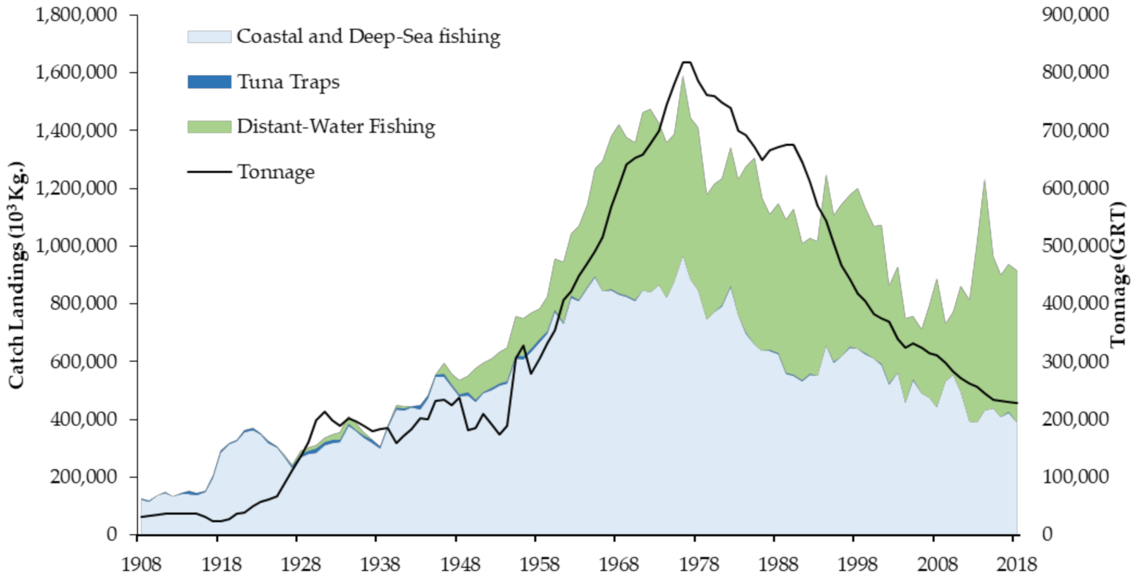
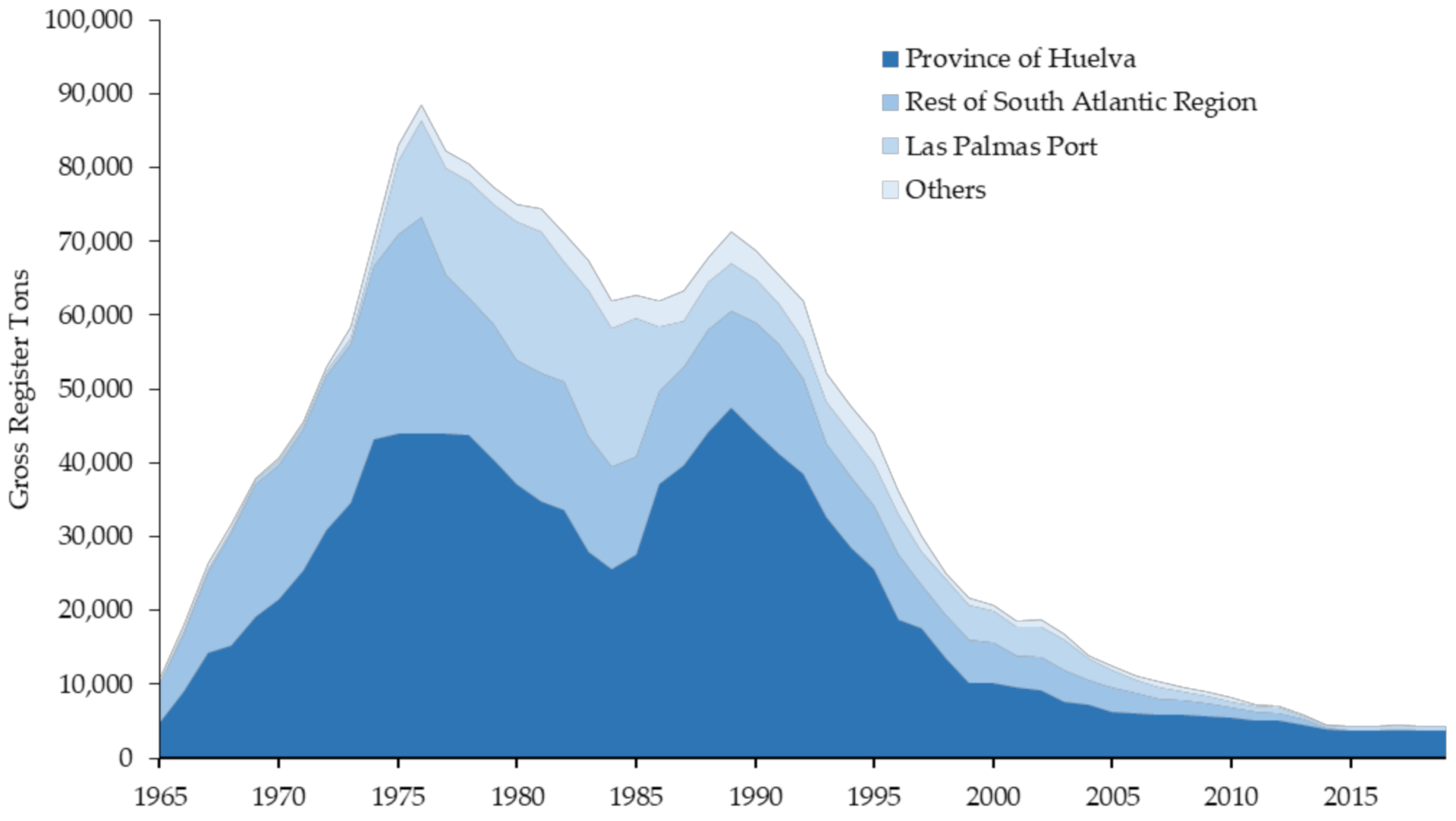
2. The Evolution of the Spanish Fishing Sector: The Crustacean Freezer Fleet

2.1. Background: The Development of Trawl Fishing

Fishing activity has always been relevant on the Spanish coast. However, the liberalisation of access to fishing activity in the 1860s spurred a major process of investment and incorporation of innovative techniques, including the introduction of the first vessels equipped with steam engines both in the Cantabrian Sea and the Gulf of Cadiz. While initially purchased overseas, later on these vessels were built in national shipyards. In 1904, almost 400 steam-powered vessels and more than 22,000 sailing and rowing boats were used for fishing [14]. Nonetheless, the majority of these were small in size; in fact, only 13 of these vessels exceeded 100 GRT. A decade later, almost 800 steam-powered vessels were used for fishing, around 60 of which exceeded 100 GRT [15]. Following the events of the First World War from 1914 to 1918, during which several vessels were sunk by German submarines and many more were sold to combatant countries for use as patrol boats and minesweepers, the fleet expanded very quickly (Figure 1). By 1920, it comprised 1569 motorised vessels—only 47 of which exceeded 100 GRT—and more than 29,000 sailing and rowing boats [16]. In 1930, there were already 5505 of the former—170 of which exceeded 100 GRT, including six large cod-fishing vessels that exceeded 1000 GRT—and more than 36,000 of the latter [17].
In 1940, following the Spanish Civil War, the self-propelled fleet consisted of 5901 vessels with a total GRT of 115,390 tonnes [18]; by 1945 there were 7692 vessels with a total GRT of 175,021 tonnes [19]; and by 1955, the motorised fleet included 10,382 vessels with a total GRT of 271,876 tonnes [20]. Many of these vessels were nothing more than old sailing or rowing boats with small combustion engines installed. The fleet also included many steam-powered vessels that had been built some decades before with clearly outdated technology. At this juncture, and in order to resolve the pressing need to find sources of food to feed the population, the modernisation of the fishing fleet was boosted through Spanish Law 147/1961 on the Protection and Renovation of the Fishing Fleet (Ley 147/1961, de Protección y Renovación de la Flota Pesquera), and also by the Fisheries Credit Society, a fundamental instrument under the first economic development plan established via decree law on 23 July 1964. Thanks to this financial and fiscal momentum, by 1970 the situation was already radically different to how it had been just a decade previously. There were hardly any sailing or rowing vessels, while self-propelled vessels—equipped with combustion engines and to a much lesser extent steam engines—now totalled 15,250 units with a total GRT of 653,191 tonnes. This process reached its peak in 1977 when the fleet consisted of 17,153 units with a total GRT of 817,524 tonnes, double the capacity existing in 1960 (Figure 1). By then it had consolidated a number of modern trawler and seiner vessels that fished in the North Atlantic, along the whole African coast and in the American Southern Cone, and had even begun to operate in the Indian and Pacific Oceans. This was quite the contrast to thirty years earlier, when only the occasional cod-fishing vessel could be found operating in Newfoundland. This process was favoured by the freedom of fishing in the majority of the fishing grounds where the fleet operated. According to Lloyd’s Register of Shipping, by 1976 the Spanish fleet had become the third-largest fishing fleet in the world, with a total GRT of 581,000 tonnes representing 7.05% of the world total.
The difficulties began later when the EEZ was extended to 200 nautical miles in the majority of the fishing zones where the Spanish distant-water fleet operated. In 1978, the Spanish government established measures to incentivise the exportation of vessels to small joint fishing ventures in coastal countries by means of a royal decree. This process was accelerated following Spain’s entry in the European Economic Community (EEC) in 1986, and above all the implementation of the Financial Instrument for Fisheries Guidance (FIFG) measures for the exportation of vessels to joint enterprises in third-party countries, not to mention the introduction of subsidies for permanent cessation of fishing activities. As a result, between 1977 and 1987 the total tonnage of the Spanish fishing fleet fell by 18.5%, a process that intensified in the following decades, with a reduction of 33.6% between 1987 and 1997, 28.7% in the next decade, and almost 27% between 2007 and 2017 (Figure 1). In 2019, the Spanish fishing fleet comprised 8100 motorised vessels with a total GRT of 228,549 tonnes; less than half the number of vessels existing in 1977, with a total tonnage amounting to just 28% of the totals recorded forty years earlier [21].
As can be seen in Figure 1, the evolution of Spanish fishing catches reflects the same dynamics. In 1920, the fleet catches had reached 400,000 Mt [22]. This figure then declined to 230,646 Mt in 1927 as a result of the sardine crisis, although it managed to recover afterwards [18], reaching a total of 408,000 Mt in 1934 [18]. Catches increased slowly following the Spanish Civil War, with around 609,000 Mt in 1946 and over 700,000 Mt in 1955 [20]. The renewal of the fleet in the 1960s led to an expansion in catch sizes. In 1964 the total catches exceeded a million tonnes, and in 1969 the fleet catches had already doubled the catches attained in 1950, with the total amount exceeding 1.4 million Mt between 1968 and 1976 [23]. From that point onwards there was a gradual decline, reaching a low point of 709,933 Mt in 2006—similar figures to those recorded forty years earlier—before beginning a slight recovery, with 912,966 Mt in 2018 [24]. However, it is important to note that a significant proportion of this recovery was due to catches by the tuna freezer fleet in West Africa, the Indian Ocean and the Pacific Ocean, given that catches by coastal and deep-sea fishing fleets had fallen by 21% since 2006.

2.2. Crustacean Fishing and Consumption

Unfortunately, until 1925 Spanish statistics did not distinguish between the types of species caught, making it difficult to determine exactly when crustacean fishing began on an industrial scale. Before the 1920s there was little mention of crustaceans, with catches of this sort being limited to spiny lobsters, European lobsters, prawns, goose barnacles and crabs caught using fishing equipment other than trawling gear and in shallow waters. The crustacean species characteristic of deep-water trawl fishing, such as shrimp and Norway lobster, were first mentioned in what is now considered the first statistical study of a scientific nature which was to form the basis for subsequent studies. The fishing statistics indicated that, due to the increase in the bottom trawling fleet and the average size of the vessels, the consumption of crustaceans (Norway lobster, shrimp, prawns, etc.) had increased, which was previously unknown [25]. Nonetheless, they could not have constituted a significant proportion of the catches, given that when Rodríguez Santamaría [26] described the activity of “trawls and pair trawls” in the south of the peninsula, both in Spanish and Moroccan waters, no mention was made of crustacean catches and the main target species was identified as being hake. In 1921, there were 35 pairs of steam-powered vessels in Malaga, seven in Huelva, two in Cadiz and four in Seville operating from the ports in the Gulf of Cadiz, making a total of 96 vessels, in addition to another 10 steam-powered vessels that operated with trawls or otter trawls. More than half of these preferred to operate in Moroccan waters.
In the fisheries statistics of 1934, the growing consumption of these crustaceans in the main Spanish cities was also indicated. In that same year, 9861.5 Mt of crustaceans were landed in Spain, of which 3651 Mt were shrimp and 1877 Mt were Norway lobster. 40% of the former and 50% of the latter were landed at the port of Huelva, with almost 67% of both landed in the ports of the south Atlantic region as a whole, including Huelva [27].
Huelva initiated its development as a base for steam-powered trawlers in 1903 with the establishment of “Sociedad Pesquera La Atlántica” (The Atlantic Fishing Company), which acquired two trawlers in Germany that would remain operative until 1916. In 1905, two pairs of steam-powered trawlers owned by Gutiérrez Feu, a businessman from Ayamonte (Huelva, Spain), were added to the fleet. All of these vessels exceeded 150 GRT. While in 1920 there were 22 steam-powered vessels in Huelva with a GRT of 652 tonnes, by 1925 there were already 44 vessels with a total GRT of 2428 tonnes. By 1930 the fleet had expanded to 69 motorised vessels with a total GRT of 4492 tonnes, and after the Spanish Civil War in 1939 there were 82 vessels with a total GRT of 6540 tonnes. These data were extracted from the annual fleet lists provided by the shipowners’ association to the chamber of commerce, industry and navigation of Huelva, along with data from the lists prepared by the fishermen’s guild. In Huelva, the yield from this crustacean trawl fleet’s fishing activity was very high due to the “high prices received for some of the crustaceans, shrimp and Norway lobster that the Huelva-based fleet had specialised in” [28]. Unfortunately, the fleet’s growth was slowed by fuel supply difficulties which persisted until 1954, along with the continued increase in fuel prices which also significantly curtailed fishing activity. Between 1936 and 1942 the price of coal increased by 300% and diesel prices increased by even more. The limited supply meant that steam-powered vessels were only able to operate around fifteen days per month and vessels equipped with combustion engines could only go out five or six days each month (report of the fishermen’s guild of Huelva dated 2 December 1942). In the mid-1950s—by which time the majority of the steam-powered vessels had already installed diesel burners—the supply was normalised and the fleet was once again able to operate at its full capacity. The result was predictable: after one or two excellent years in terms of catches, in around 1955 the yields began to fall and there was a rapid decline in the landings of fresh crustaceans, the majority of which came from the fishing grounds in the Gulf of Cadiz, reaching its lowest level in the late 1960s (see Figure 2). While 22 million kg of fresh or chilled crustaceans were caught in 1955, during the following decade the landings fell by 60% throughout Spain, with a slightly bigger drop in the south Atlantic region (61.3%) and even lower for the port of Huelva, which fell by 67.8%. This latter port, which represented half of the national total in 1955, continued to fall progressively, and by 1969 it accounted for only a fifth of the landings of fresh or chilled crustaceans.
The reasons for this steep descent were twofold: the trawler fleet in the Gulf of Cadiz, especially in Huelva, focused its efforts on crustaceans, alternating fishing trips between the waters of the Gulf of Cadiz and the north of Morocco (5 and 15 days away from port, respectively). The replacement of coal with other fuels accelerated this process, allowing the fleet to go on longer trips and increasing its catch load capacity. Due to overfishing in the Gulf of Cadiz, the option of operating in Moroccan fishing grounds became the ideal solution for the trawler fleet. However, after achieving independence in 1956, Morocco began to impose limitations on the activities of the Spanish fleet and seized vessels on a regular basis, with the first bilateral fishing agreements being reached in the mid-1970s.
Faced with this situation, and thanks to the incentives introduced by Spanish Law 147/1961 on the Protection and Renovation of the Fishing Fleet, a process was initiated to restructure the fleet on two different levels: on the one hand, a large number of smaller obsolete vessels were substituted with larger wet-fish trawlers; and on the other hand, modern freezer vessels began to be built for crustacean fishing in waters located increasingly further afield. This process gave rise to the subject of this paper, the crustacean freezer trawler fleet, which had its origins in January of 1964 when the Onuba, a trawler built in 1958 that was adapted in 1963 to install freezing chambers, landed 50 tonnes of frozen fish and several more tonnes of fresh fish caught in Senegalese waters in the port of Huelva.
The Lemus and the Andrade owned by the Galician company Pescanova, the first freezer trawlers to operate both in Spain and worldwide, completed their first trips in 1961. Although these vessels mainly focused on hake and other groundfish, they also landed significant amounts of crustaceans among their bycatches. The success of these early freezer trawlers led to the construction of new vessels, a process that was spurred on by the incentives established in Spanish Law 147/1961. In only ten years, more than 60% of the Spanish fishing fleet’s tonnage had been renovated by incorporating innovations to both fishing gear and detection and communications equipment. In particular, deep-sea and distant-water fishing vessels also became larger, thereby allowing expansion of the fleet’s operating radius.
At the beginning of the 1970s, more than 90% of the Spanish freezer fleet was made up of trawlers, of which 46% had their home port in the South Atlantic region. Huelva had established a considerable freezer fleet specialising in crustacean fishing and operating along the whole African coast between Mauritania and Mozambique. Another part of the fleet based in Cadiz operated in Senegalese and Mauritanian waters, specialising in Benguela hake fishing. The northwest region also had an important trawler fleet based in Galicia, which focused more on cephalopods from the Saharan Bank, along with hake and other groundfish from the waters of Namibia and South Africa.
The first year the official statistics recorded significant landings of crustaceans by the crustacean freezer fleet was 1964, with around 38 Mt. However, only three years later the crustacean landings from this fleet already exceeded 10,000 Mt, going on to reach 14,000 Mt in 1969. The series has been reconstructed using the reports issued by port authorities from two different periods (1965–1967 and 1982–1985) [28]. The growth of the crustacean freezer trawler vessel segment was driven by credit facilities and the existence of a large market accustomed to consumption of this product. This market was willing to pay high prices, allowing the segment to obtain very high returns.
Between 1975 and 1985 many vessels moved their base to the Canary Islands, given that based on the terms of the Madrid Accords it was thought this would allow them free access to Moroccan and Saharan waters without having to pay any fees. Nonetheless, this did not change the fleet’s activity in any way as they continued to fish in an uninterrupted manner in the same fishing grounds, with their catches reaching the peninsula via carrier vessels. After Spain joined the EEC, they moved their vessels back to their home ports on the peninsula so that they could benefit from the incentives of the CFP (Figure 3). In any case, over the course of its life the Spanish crustacean freezer fleet had its main base in the port of Huelva.
The first major crisis of the Spanish crustacean freezer fleet occurred years later when the EEZ was expanded to 200 nautical miles. This resulted in the nationalisation of 95% of the marine resources, with considerable restrictions being placed on access to the fishing grounds where they had traditionally operated, thereby radically transforming fishing activities. The partial solution to this problem was the creation of joint fishing ventures (JFVs) through Spanish Decree 2517/1976, which promoted exportation of fishing vessels as a means of ensuring continued access to the resources of third-party countries. Between 1977 and 1985, 20% of the Spanish industrial fishing fleet, the main component of which was the freezer trawler fleet, was exported to JFVs to benefit from tariff-free import quotas and other incentives. Following Spain’s admission to the EEC in 1986 until the end of the 1980s, the fleet managed to recover to a certain extent. However, the introduction of the concept of joint enterprises under the community acquis and the restrictions on access to fishing grounds of third-party countries led to the transfer of a considerable part of the fleet to countries such as Angola, Senegal, Mozambique, Argentina and Chile, among others, and between 2003 and 2019 the crustacean freezer fleet was halved.
To sum up, at the height of its activity—around 1990—the crustacean freezer fleet constituted a significant segment of the Spanish fishing sector, representing 3% of total catches in terms of weight and 17% in terms of value and accounting for 10% of the Spanish fishing fleet’s tonnage. Nowadays, and following a severe adjustment, this segment consists of a mere 31 vessels totalling 7980 GT (around 4299 GRT) with annual catches that barely exceed 5000 Mt. This represents only 0.5% of the total weight of landings by the Spanish fishing fleet, 2.7% of their value, and only 1.9% of the Spanish fleet’s tonnage in 2019.

3. Methodology

3.1. Background and Theorical Basis

Without a doubt, one of the transcendental elements of the neoclassical theory of capital is the role played by physical capital as an essential input to understand productive processes. There seems to be a general consensus regarding the empirical consideration and adequate measurement of production and the work factor; however, there is less consensus regarding the role of physical capital as a productive input which must inevitably be quantified taking into account its nature as stock in a dynamic environment over the course of its service life. In order to study the investment mechanisms and the characteristics of capitalisation, a useful source of information that permits the study of economic growth is required. Capital accumulation strategies are often applied not for purposes of business efficiency and productivity but rather for speculative reasons. Accordingly, the correct measurement of capital stocks, investment flows (gross fixed capital formation) and depreciation (consumption of fixed capital) in a specific productive sector is essential to ensure accurate assessment and diagnosis of the situation, thereby allowing implementation of effective economic policy measures.
Considered as the physical determinant of the production possibilities in a specific productive sector, the capital stock of a production unit at a specific point in time may be defined as the result of the accumulation of investment flows that have taken place during the current period and in previous periods which still remain in stock. Therefore, capital stock consists of all long-lasting fixed assets that are engaged in the productive process and that are used repeatedly over time.
Since the first studies addressing this topic, the approaches to the concept of capital stock and its estimation have undergone significant changes in terms of their methodology and focus. The starting point for all of these studies is the work by Jorgenson [29], who proposed that the rate of depreciation of capital assets is a constant proportion of the capital stock at any given moment. However, many authors were very critical of the proportionality hypothesis proposed by Jorgenson [30,31,32]. While in the past the problem focused on the endogenous estimation of the optimal service life of different types of assets, this vision of the depreciation rate considers an exogenously predetermined average service life. In order to consider depreciation as a variable in economic/business decision-making, we need to be able to define its correct economic measurement. In fact, a number of empirical studies estimated economic depreciation based on the prices of the different assets on the second-hand market [33,34]. Others obtained the economic value added of the net capital stock by introducing a corporate valuation ratio [35,36,37] while Escribá, Ruiz and Murgui [34] incorporated the depreciation rate in the set of decision variables. Some empirical studies use second-hand markets and geometric depreciation functions to determine the age-price profiles of different assets.
Different contributions have also been made by international organisations such as the OECD which seek to ensure methodological standardisation. The OECD Manual ‘Measuring Capital 1992’ [38] considered two versions of capital measurement based on the work by Ward [39], gross capital stock and net capital stock, with particular emphasis on the breakdown by productive sectors for private capital and the functional breakdown for public capital. Subsequent versions of the above OECD manual [36] included contributions by Jorgenson and Griliches [37], who considered that capital stock is divided into three levels: gross capital stock, productive capital stock and net capital stock. The approval of a new System of National Accounts in 1993 (SNA 1993) and its adaptation to EU countries through the European System of Accounts (ESA 1995) resulted in the need for modifications to the methodology used in this new environment [3], continuing to consider the three types of capital stock already established in previous works while also recommending the use of geometric patterns for depreciation. Therefore, three fundamental variables were established: investment, capital and depreciation, all of which are strongly linked to capital measurement. The most common capital valuation procedure is the perpetual inventory method (PIM), developed by the OECD, which estimates the capital stock series at the replacement price taking into account both investment and depreciation flows. This methodology requires a sufficiently long investment series and estimates of the service life of the capital assets, along with selection of a survival (or geometric depreciation) function for those assets. The basic idea is to interpret an economy’s capital stock as an inventory that increases with capital formation. There are methodological differences with regard to the method of estimating the initial capital stock. Harberger [40] argued that the output grows at the same rate as the capital stock. In 1980, Griliches [41], presented another approach that was refined by De La Fuente and Domenech [42] who argued that growth rate of the capital stock can be approximated by the growth rate of investment. Later, Jacob, Sharma and Grabowsky [43] and Kamps [44] made a forced time series of investment.
There are numerous empirical applications for capital measurement in the economic literature which have estimated capital stock series for different countries over different periods of time [33,44]. Capital stock series have also been estimated at a regional level [34].
In this paper, we have used the information on depreciation that is implicit in the asset prices in successive sales, estimated using econometric techniques. To make these estimates we needed to know the prices of the new and second-hand assets in different periods. We followed the approach adopted by Hulten and Wykoff [45], who used a single depreciation rate per asset for the industry as a whole, without distinguishing between productive sectors or companies, considering the geometric form to determine the age-price profile of the assets as they age. Baily, Baily and Gordon and Baily and Nordhaus used alternatives depreciation rates [46,47,48]. Other authors applied information from asset disposal surveys, assuming a geometric depreciation [49].

3.2. Model to Obtain the Age-Price Profile of Assets

In the economic literature, there are the different approaches that analyse assets depreciation rates. The main empirical work in this field was carried out by Hulten and Wykoff, in 1981 [45]. Later, other authors have presented some studies by this approach [50,51]. In general, these econometric models estimate the age-price profile of an asset as follows (model 1):
ln P i n , v , t = a + β D n i + γ D v i + μ D t i + ε i
where Pin,v,t is the price or valuation of the asset i; α, β, γ and μ are the parameters to be estimated, εi is a random disturbance term and Dni, Dvi and Dti are explanatory variables. The variable Dni indicates the age of the asset i at the time the transaction takes place, while the parameter β represents the impact on the asset’s price as its age increases. When applying the model (1) to the fleet, Dvi represents the year the vessel i was built and the parameter γ represents the impact of the vessel’s technical configuration when it was built on the price it reached in the transaction. Dti represents the year the transaction took place and the parameter μ is considered as an estimate of the price index for new assets, with the quality remaining constant. The parameter β is very closely linked to the phenomenon identified by Akerlof [52] occurring in certain second-hand markets and successive sales. This author analysed market situations in which the purchasers are unable to evaluate the quality of the assets in the transactions, affirming that when purchasers assume the market has been invaded by lower quality goods (named lemons) they offer low prices, but this drop in prices also affects higher quality goods, which will end up being sold at a lower price, therefore meaning that the prices attained in those transactions are not representative of the prices of similar assets that are not sold.

3.3. Obtaining the Age-Price Profile of Vessels of the Crustacean Freezer Fleet

The application of the perpetual inventory method to measure the capital stock of a fishing fleet involves estimating the gross value of the capital stock of a vessel at a certain age based on the purchase value of new and second-hand vessels. The productive capital stock is estimated by applying the age-price profile to the vessel replacement value. When the depreciation follows a geometric pattern, the net capital stock is equal to the productive capital stock. By adding up the value of the net capital stock of all of the vessels in the fleet each year, we obtain the total net value of the fleet. The starting point to obtain the value of the capital stock of the fleet is the estimation of the gross fixed capital formation.
There are precedents in this sense. Applying a model based on Hall’s work [53], Lee [54] estimated the capital of the Japanese fishing fleet using the insured value of the vessels against total loss as a proxy for the acquisition prices. Based on Kirkley and Squires [55], Del Valle and Astorkiza [56] analysed the value of the fishing fleet in the Basque Country, using private data from 228 transactions in the second-hand market. These works were based on the hedonic price theory, which in this context and also for the purpose of this study, considers that the vessels have a set of attributes each of which is characterised by a shadow price, with the combination of these determining a vessel’s sale price. The first studies date back to 1960s [57,58,59,60]. The application of the hedonic price methodology supposes the construction of an econometric model that determines the functional relationship between the price of the good and its respective characteristics. To do this, the relevant variables are previously identified and the necessary database is built for the implementation of the econometric procedure that leads us to identify the hedonic equation.

4. Statistical Information

One of the main results of this study is the determination of the capital stock time series for the Spanish crustacean freezer fleet. Nonetheless, the information obtained on the technical, economic and financial characteristics of the fleet over a period of more than 50 years is equally important, given that there is no single statistical source for the list of vessels that formed part of this fleet.
La Flota Pesquera Española (The Spanish Fishing Fleet) was the publication used for the period from 1965 to 1972, which included a complete census of the fleet at the end of each year. From 1973 onwards, statistical data aggregated by port, category, age and tonnage were included in the Anuarios de Pesca Marítima (Maritime Fishing Yearbooks). Continuing from the lists available for 1972, we were able to reconstruct the series. The last yearbook was published in 1986. However, as from 1989 we had access to the Census of the Operative Fishing Fleet (CFPO) prepared by the Ministry of Agriculture, Fisheries and Food (MAPA), which made it possible to link the series. We also extracted information from the Lista Oficial de Buques (Official List of Ships), an annual publication with comprehensive lists of the Spanish merchant and fishing fleet, including technical data on the vessels and the shipowner companies. Along with these official sources, we also used information available from 1970 onwards in the annual censuses of vessels affiliated with the National Association of Crustacean Freezer Vessel Owners (ANAMAR), the association for this segment of the fleet. The series was completed with census information supplied both by MAPA and the regional government of Andalusia, which included lists of subsidies for new constructions in different invitations to tender. Finally, we obtained relevant information from the vessel registers of different maritime authorities and in particular the commercial registry of Huelva. This provided us with access to technical, economic, financial and legal data regarding many of the vessels and their owners. It also gave us important information on any economic transactions during the lifetime of these vessels, distinguishing between the different types of transaction—sales to third parties, sales to companies of the same group and tenders—with the former being used in the estimates given that the remaining transactions were clearly below market value either for fiscal reasons or reasons of expediency. Other sources used to validate the data were the Community Fishing Fleet Register and the FAO Fishing Vessels Finder, as well as different public and private databases like www.wrecksite.eu (accessed on 17 September 2020), www.histarmar.com (accessed on 13 November 2020) and www.marinetraffic.com (accessed on 7 December 2020) and the organization named Fishsubsidy.
This information was gathered and filtered to create a database of 500 vessels containing 7550 records and more than 377,000 entries. This was then used to carry out an in-depth analysis of the evolution of the fleet being studied, especially the relevant variables for estimation of capital stock series and gross fixed capital formation, along with information regarding the vessel’s ownership, corporate group, home port and the different types of public and private financing the vessel had access to for each of the years analysed. Given that we were dealing with values referring to different periods of time, we expressed statistical information of a monetary nature in real terms using the gross domestic product (GDP) deflator, more specifically one of its four components: the gross fixed capital formation (GFCF) deflator, taking 2011 as the base year.

5. Results

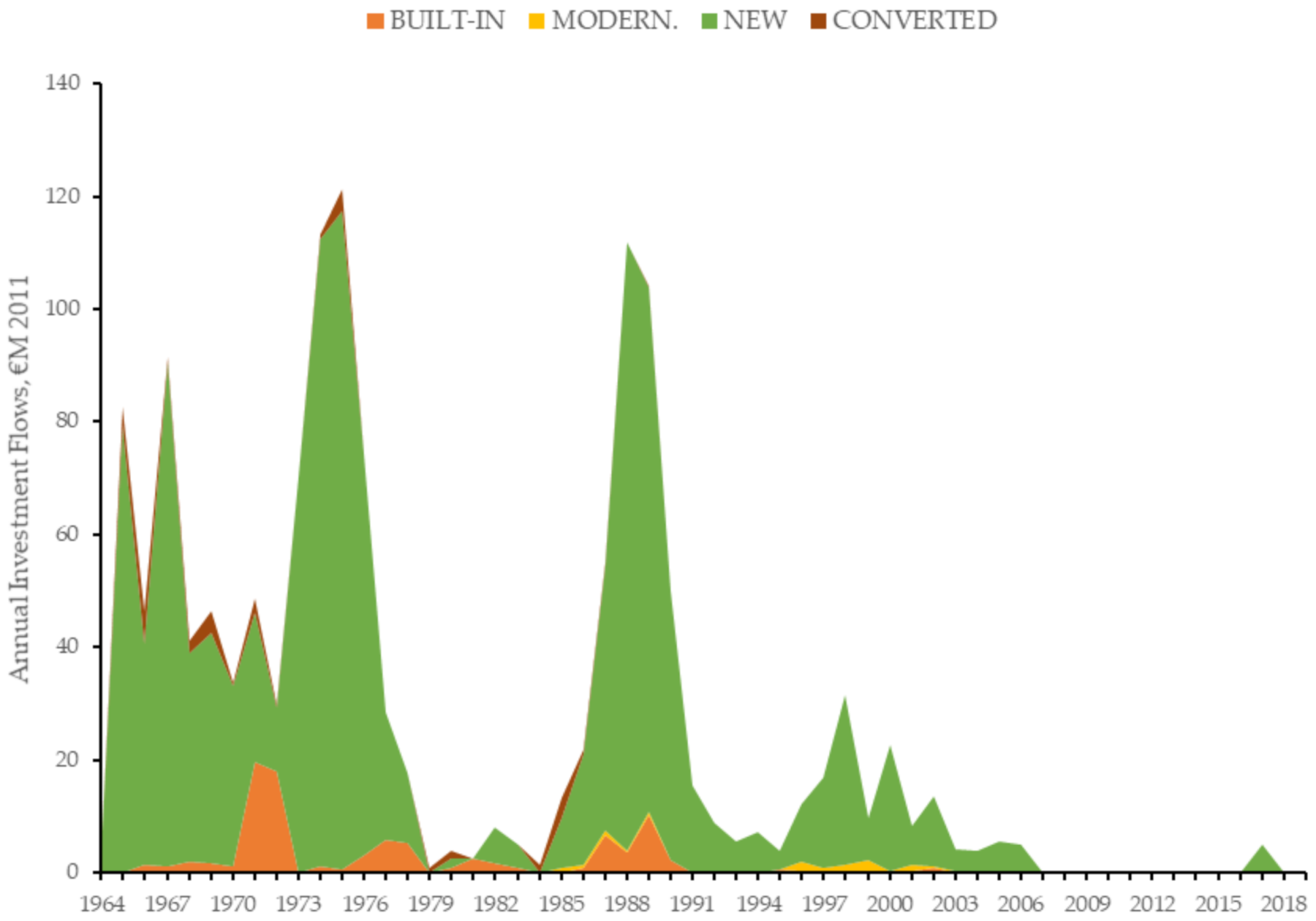
5.1. Estimation of the Gross Fixed Capital Formation

Using the information gathered, a total of seven quantitative variables were selected relating to the vessel’s technical and economic characteristics. We included some dummy variables that represented distinctive features such as whether the vessel had been built as a freezer vessel or whether it was a wet-fish vessel that was subsequently adapted and some other variables representing the shipyard where it was built. The description of each variable (Table 1) is as follows: Y: building value; X1: tonnage; X2: engine power; X3: overall length; X4: beam; X5: length between perpendiculars; X6: hold depth; R: A wet-fish vessel that was subsequently adapted; A1: Astilleros de Huelva, S.A.; A2: Astilleros Armón, S.A.; A3: Astilleros del Atlántico, S.A.; A4: Astilleros Balenciaga, S.A.; A5: Hijos de J. Barreras, S.A.; A6: Construcciones Navales Paulino Freire, S.A.; A7: Astilleros La Parrilla, S.A.; A8: Astilleros Neptuno, S.A.; A9: Astilleros Ojeda y Aniceto, S.A.; A10: Astilleros Ría de Avilés, S.A.; A11: Astilleros Zamacona, S.A.; A12: Construcciones Navales del Sureste, S.A.. The market situation in each of the shipyards, their technical and economic characteristics and the different technologies used had a certain impact on the vessel’s value. One of the dummy variables initially included in the study referred to the hull material. Of the total sample of 267 vessels, only three of them had a wooden hull. The analysis of the outliers indicated such vessels as rare points, so these records were eliminated, thus discarding this variable.
To specify the functional form that best explains the investment or gross fixed capital formation that was carried out each year and under the hedonic price theory approach, the construction value of a vessel in this fleet was estimated starting from a flexible functional form (translog production function) in the variables related to the technical characteristics, not in the dummies, in order to define the different factors that determine the price of a good, in this case, the price of building a vessel [61]. Considering a sample of N = 267 vessels, we could use the following model (2) to obtain an estimation of the construction value of a vessel in this fleet:
ln Y i = α 0 + k = 1 4 α k l n X k i + 1 2 k = 1 4 j = 1 4 λ k j   l n X k i l n X j i + δ R i + s = 1 12 ϑ s A s i + ε i   ( i = 1 , , N )
where Yi is the construction value of vessel i; αk (k = 0, …, 4), λkj (k,j = 0, …, 4), δ and ϑs (s = 1, …, 12) are the parameters to be estimated, εi is the random disturbance term and Χki, Ri and Asi are explanatory variables. Xki are related to the vessel’s technical characteristics. Ri indicates whether the vessel had been built as a freezer vessel or whether it was a wet-fish vessel that was subsequently adapted and Asi is the shipyard where it was built. α0 is the intercept and αk represents the impact on the vessel’s price as this characteristics increase. λkj is the parameter associated with interaction term. δ indicates the effect on the construction value that the vessel were a converted wet-fish vessel and ϑs represents the impact on the vessel’s value due to the market situation in each of the shipyards, their technical and economic characteristics and the different technologies used.
A flexible functional form was adequate because it does not impose many a priori restrictions, which is why they are usually chosen by many authors [62,63,64]. We only imposed a priori the symmetry restriction in order to be able to identify the coefficients γij = γji. From the translog function (2) we applied different hypothesis tests allowing us to discriminate the correct functional form [65]. Homogeneity tests, constant returns to scale, weak overall separability, weak linear separability [66], and weak nonlinear separability (Table 2) were included. After accepting homogeneity and weak global separability, the resulting model was a Cobb–Douglas function. The contrast on constant returns to scale recommended the rejection of the null hypothesis, so that a proportional increase in all the inputs of the model did not translate to the same extent in the endogenous variable.
Once the Cobb–Douglas functional form was accepted as adequate and from an initial sample of 267 vessels, a regression analysis was carried out using the ordinary least squares procedure. The preliminary analysis of the set of variables in the model let us detect the existence of a strong multi-collinearity between the variables related to the technical characteristics of the vessel. The condition index presented a value much higher than 20 [67]. Pearson’s linear correlation coefficient between the technical variables reflected high levels of correlation.
The explanatory capacity of the model is 87.15% and since our objective was predictive, this resulting model could be used. However, the existence of strong indications of multi-collinearity could make it difficult to correctly interpret the contributions of each characteristic of the vessel to the construction value or implicit prices. To eliminate that, we chose to transform the regressors relative to the technical characteristics of the vessel by means of a factorial analysis in principal components, obtaining four orthogonal factors that sufficiently explain the original variables. The rotation method improved the ability to interpret the factors. To obtain the orthogonal factors, different rotation criteria were applied and, based on the results obtained, the Equamax rotation method with Kaiser normalization [68] was selected, as it is the one that offers a more informative and interpretable factorial solution. Component PC1 collected especially the influence of the beam of the vessel, PC2 is mainly identified with the power of the vessel; the third component largely accumulated the incidence of tonnage measured in GRT units and, finally, the last component reflected the influence of the overall length of the vessel.
From the correlation matrix, the set of indicators was obtained and hypothesis tests were carried out to verify the suitability of the application of this technique. Next, the estimation of the function provided the construction value of a vessel in this fleet was performed again, under the Cobb-Douglas functional form and incorporating the four orthogonal factors, as well as the dummy variables initially included.
Both the significance of the variables and the model as a whole as well as the possible existence of residual observations were analysed. There were three dummy variables excluded from the model as they were not significant, and they were those related to shipyards number 2, 8 and 11, which represent three shipyards that had a lower presence in the construction of this type of vessels). The analysis of the outliers reflected the existence of observations with especially high residues that correspond mainly to vessels, mostly built at the end of the 1950s for fresh fishing, some of them with a wooden case, and which were later reconverted to frozen [69,70]. The final sample consisted of a total of 248 observations.
After verifying the existence of heteroscedasticity, the estimated variance-covariance matrix of the estimators was corrected using White’s asymptotic transformation. Considering a sample of N = 267 vessels, we used the following model (3):
ln Y i = α 0 + k = 1 4 α k P C k i + δ R i + s = 1 12 ϑ s A s i + ε i   i   = 1 ,   ,   N  
where Yi is the construction value of vessel i; αk (K = 0, …, 4), δ and ϑs (s = 1, …, 12) are the parameters to be estimated, εi is a random disturbance term and PCki, Ri and Asi are explanatory variables. The variables PCki are the factors obtained after applying the factorial analysis in principal components and they collect the influence of several technical characteristics of the vessels; Ri indicates whether the vessel had been built as a freezer vessel or whether it was a wet-fish vessel that was subsequently adapted and Asi is the shipyard where it was built. The resulting model, the construction value of each vessel i is explained from the four main components obtained, representative of the beam, the GRT, the power and the total length. αk represents the positive impact on the vessel’s price as this characteristics increase; δ indicates the effect on the construction value that the vessel were a converted wet-fish vessel and ϑs represents the impact on the vessel’s value due to the market situation in each of the shipyards. The adjusted R-squared value (87.15%) indicated a high explanatory capacity of the model. The specific form of the resulting model (Table 3) allowed us to verify that successive increases in inputs cause a positive marginal effect on the reference construction value for each vessel, keeping the rest of the explanatory factors constant. The model included dummy variables that helped to improve its predictive capacity by including the impact of qualitative factors on the vessel’s construction value. Finally, the explanatory variable Ri had a negative effect on the construction value.
These were initially cheaper vessels; however, their subsequent adaptation increased the reinvestment flow. Nine additional dummy variables were included representing the shipyard where the vessel was built, which had parameters of differing values. For example, the variable A1 representing Astilleros de Huelva, S.A., where a large number of the fleet’s units were built, had a positive effect on the vessel’s value. In contrast, others such as A3 corresponding to Astillero del Atlántico, S.A. in Santander resulted in significantly lower construction values than the estimated average levels.

5.2. Valuation of the Gross Fixed Capital Formation

Once the model had been estimated, we began to prepare the construction value predictions for the cases in which these data were unknown. The annual investment or gross fixed capital formation for the fleet from its beginnings through to the present day includes the construction value, real or estimated, of the built freezer vessels that are immediately incorporated into the fleet (new), the market value of the vessels that are incorporated into the fleet from another fishery (built-in), the market value of fresh trawlers previously built and later converted into freezers (converted) and finally the value of modernization investment in this fleet (Figure 4). The market value of the vessels has been estimated according to model (4) included in Section 5.3.
As can be seen in Figure 4, from 1964 until the mid-1970s the levels of annual investment in this fleet were generally very high, due to the introduction of legislation that enabled upgrading of the majority of the obsolete vessels. The maximum values were reached in 1975. Those were the years in which the demand for crustaceans increased exponentially in the Spanish market; in 1965 the apparent per capita consumption was slightly over 0.6 kg/head/year, but by 1970 it had increased by 40%, and by 1975 it had gone up by a further 80%, with a per capita consumption of 1.55 kg/head/year. In comparison with the market volume of 19,700 Mt recorded in 1965, by the next decade this had reached a total of 55,284 Mt, during a period in which almost all of the offer came from fishing activity with negligible amounts of imports. This increased offer did not result in a price decrease. In fact, during this decade an over-valuation of 70% was experienced in real terms, which may be explained by the improved levels of disposable income and quality of life in Spanish households. As a result, there were strong incentives for investment. This trend slowed down from 1978 onwards due to the extension of the EEZ to 200 nautical miles and the economic crisis suffered in Spain.
The exportation of vessels to joint fishing ventures favoured access to the resources of third-party countries by many of the vessels in this segment, with many being exported to Argentina, Panama, Senegal and Morocco between 1978 and 1982. Nonetheless, it also generated strong flows of imports, firstly due to the quotas granted to the JFVs and later in a more widespread sense. Between 1975 and 1985 the apparent consumption of crustaceans continued to increase, reaching a total market volume of 65,776 Mt in 1980 and 70,781 Mt in 1985. There was also considerable growth in the percentage represented by imports, rising from 5% in 1975 to 30% in 1985. These imports had a considerable impact on first-sale prices, meaning that in real terms these were devalued by 30% during this decade. The fleet had to deal with a sharp increase in costs, not only of fuel, which tripled in price during this period, but also the licences imposed by coastal countries following the expansion of the EEZ zone. Many vessels did not obtain these licences and a number of shipowners went bankrupt.
Given the situation faced by the sector, in 1986 the regional government of Andalusia promoted the construction of 15 vessels to substitute the part of the fleet that was considered outdated, accounting for the upturn that can be seen in the series. In addition, several freezer vessels built after Spain joined the EEC were added to the fleet, particularly during the period from 1989–1991. However, many of these units later accepted subsidies for the exportation of vessels to joint enterprises, meaning that fleet numbers continued to fall, with only a few minor investments in 2004–2005. During this period, the per capita consumption of crustaceans continued to increase. By 1990, it had reached 3.16 kg/head, reaching a maximum level in 2006 of 4.7 kg/head, with a total traded volume of 207,256 Mt, of which only 7.7% corresponded to catches from the fishing fleet, with the majority being imports from third-party countries. In real terms, the average price at first sale remained around the 1985 levels due to the mass entry of imports. Evidently, there were hardly any incentives for investment; in fact, the situation was quite the opposite. What is surprising is that two new vessels were built as late as 2017.

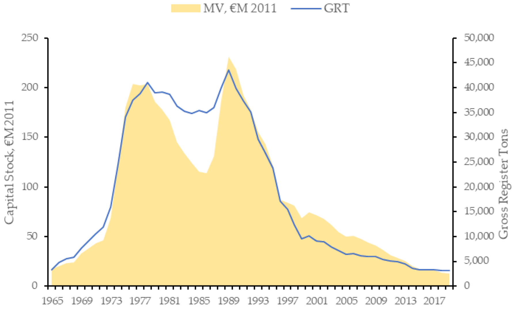
5.3. Estimation of the Capital Stock of the Fleet

To obtain the capital stock, a ratio was required allowing evaluation of the asset depreciation process, and, in particular, estimation of the age-price profile of the vessels, in order to determine the evolution of the vessel’s value in each year of its service life. Following Hulten and Wykoff’s approach [46], the model considered the most significant as a whole was the one where the vessel’s value was estimated by taking into account its construction value, age, year of construction and power. A Box-Cox transformation was used to demonstrate that logarithmic transformation was the most suitable means of transforming the dependant variable. Accordingly, if the value of vessel i in second or subsequent sales in year t is Yitsh, the construction value (real or estimated according model 3) of the vessel i is Yi, the age of the vessel i the year t is T1it, the engine power of the vessel i the year t, is T2it, the year of construction of the vessel i is T3i and εit is the random disturbance term, the model used to estimate the depreciation process for the vessel i over the course of its service life would be as follows (model 4):
LnY it sh = α 0 + α 1 LnY i + α 2 T 1 it + α 3 T 2 it + α 4 T 3 i + ε it ( i = 1 ,   ,   N )  
where αk (k = 0, …, 4) are the parameters to be estimated. The information on successive sales (167 sales) was available for a limited sample of vessels (N = 107 vessels). The estimated model with this sample (Table 4) had an explanatory capacity slightly higher than 85%, as measured by the adjusted R-squared. Once the model had been estimated, Ramsey’s RESET test was applied to determine whether the functional form used could be considered incorrect. In this case, the value of the statistic was 0.0605 and its p-value was 0.806, indicating that the null hypothesis could not be rejected. It was therefore considered that the model’s functional form was not erroneous.
For the variable Yi a positive elasticity (0.760) was estimated, which predicted a positive percentage increase of less than one in the vessel’s market value in the event of a unit percentage increase in its construction value; a fairly obvious result due to the market trend of assigning a market value to a vessel that is positively related to its construction value. The variable T1it, which represented the age of the vessel i the year t, had an estimated coefficient of −0.0554, allowing quantification of the loss of value recognised by the market as its age increased. The model predicted that for each year a vessel’s age increased, the market value would be reduced by 5.54%, assuming there were no other factors influencing the depreciation of the vessel. The vessel’s power T2it which was closely related to its fishing capacity, was another relevant variable used when assigning the market value of each vessel. The value of this variable may have increased or decreased depending whether the vessel had undergone any refurbishment work during the period analysed. As was to be expected, the coefficient for this variable was positive, which was indicative of this fact. The estimated model was used to determine a vessel’s age-price profile over the course of its service life. For the purposes of this research, this was considered as the period during which it formed part of the fleet, with vessels built as freezer vessels being considered separately to other types of vessels that were later adapted for this purpose. In the first of these two cases, the vessel’s value in the first year was its construction value and from the second year onwards its value was estimated using the corresponding model. Meanwhile, in the second case the vessel’s value was estimated for each of the years it formed part of the fleet using the model. The depreciation rate for both types of vessels from the second year onwards was 5.3%, in accordance with the geometric model.
The capital stock of the fleet as a whole was estimated by adding the estimated values of the active vessels in each of the years analysed. As reflected in Figure 5, after the intense capitalisation of the exceptionally large fleet during the first years, from 1978 onwards its market value decreased drastically and it never recovered. However, by quantifying the fleet based on the tonnage or the number of units, it can be seen that the fleet recovered to a certain extent, leading to an erroneous interpretation of the capital invested in the fleet.
Once the net capital stock of the crustacean freezer fleet had been estimated, it was possible to determine the annual net investment in this fleet, understood as being the difference in the capital stock between consecutive years. Figure 6 shows the annual series of net investments made in the fleet, taking into account the value of new units added to the fleet, the depreciation suffered by vessels that remained in the fleet and the units removed from the fleet, whether due to dismantling, sinking or exportation.
The first vessels of the freezer fleet were the starting point for the initial gradual and subsequent rapid growth of investment flows: while in 1966 the segment had 41 vessels, ten years later this figure had increased to 241. As a consequence of this heavy capitalisation, the fleet reached very high levels of capital stock, with the maximums being recorded in 1976 and 1989.
This stage of growth was followed by another period with a notable lack of investments in the fleet. The extension of the EEZ to 200 nautical miles led to a change in the international maritime scenario, with the introduction of severe access restrictions in the fishing grounds where this fleet had operated. As a result, they began the process of exporting units to Joint Fishing Ventures. Between 1977 and 1985, 231 vessels from the Spanish industrial fishing fleet with a total GRT of 120,418 tonnes were transferred to 122 joint fishing ventures. Figure 6 reflects the massive decrease in net investment during this period. Despite Spain’s entry to the EEC, 10 further joint fishing ventures were created in the late 1980s, involving transfer of 14 vessels, resulting in very high divestment levels from 1989.
The newly built vessels that were added to the fleet, which also benefited from significant subsidies, were still unable to compensate for the units that had left the fleet, meaning that in the 1990s net investment levels remained in negative figures. Between 1994 and 2004, a total of 171 fishing vessels were exported through joint enterprises. In 2004, the CFP funding for construction of new vessels and transfer of vessels to third-party countries was discontinued. From that point onwards, the Spanish crustacean freezer fleet continued to gradually decrease, with only minimal additions being made to the fleet. Accordingly, the net investment levels were negligible with the sole exception of 2017, when two new vessels were added to the fleet.

6. Discussion

This paper has tried to carry out a deep reflection on sustainability of fishing resources. When the degree of exploitation of fishery resources increases, the size of the stock is reduced and the catches as well, so that the level of capital stock that could be adequate with a greater quantity of stocks becomes excessive, causing an excess of capital (overcapitalization). For this reason, the agents responsible for fishing policies must implement the necessary measures to avoid it.
An effective fishery management would guarantee the sustainability of the resource and the sustainability of the fishery, both from a biological and economic perspective. To do this, we must have tools that allow a real measurement, in monetary terms, of the excess catch capacity.
This research has carried out a reliable measurement of the capital stock of the Spanish freezer trawler fleet engaged in the capture of crustaceans and the investment flows that determine the rate of capital accumulation for the period from 1964 to 2019. We have followed a methodology based on the permanent inventory method, developed by the OECD, which is the most widely used methodology for measuring capital stock series [34,37,70].
Considering that investment decisions are made one, two or three years in advance of the moment when risks of overexploitation begin to appear, they are difficult to alter. For this reason, most of the fisheries that are overexploited end up being fisheries with a very strong excess capital and therefore an excess of fishing capacity. The excessive growth of a specific type of fishing fleet due to higher yield expectations can lead to a severe problem of overcapitalisation of the fleet in the medium and long term as a result of continued investment.
We have estimated the construction value of vessels to measure investment flows. The construction value has been calculated on the basis of its technical characteristics, whether the vessel comes from a conversion process from fresh to freezer and the shipyard where the vessel has been built. Successive increases in inputs cause a positive marginal effect on the reference construction value for each vessel, keeping the rest of the explanatory factors constant.
The estimation of the construction value of a vessel, as a preliminary step for the quantification of the capital stock of a fleet is novel approach. Definitely, the necessary compilation of detailed vessel-by-vessel data on the construction value, in our case carried out in the commercial registry of Huelva was a particularly extensive and laborious task.
Once the construction value was estimated, we proceeded to obtain the investment flows whose profile reflects the different periods of investment and divestment carried out in this fleet, essentially motivated by changes in EEZ, which was extended to 200 nautical miles in the majority of the fishing zones where the Spanish distant-water fleet operated and in the context of the Spanish fisheries policy and European Union’s Common Fisheries Policy.
Considering the loss of value due to depreciation, an econometric model has been estimated to obtain the market value of a vessel in this fleet over the course of its service life, understanding this as the time that the vessel has remained in the fleet. In the proposed model, the market value of a boat in this fleet is a function of its construction value, its age, the engine power and the year of its construction.
The model predicts a positive elasticity for the variable that represents the construction value in the vessel’s market value and a negative elasticity for the variable that reflects the loss of value recognised by the market as its age increased. As was to be expected, the coefficient for the engine power variable was positive. Finally, the inclusion of the construction year, could also be considered redundant a priori, given that the age of the vessel is also included. However, the decision was made to include both variables because the year of construction also reflected differences in terms of the equipment and technological features and the coefficient estimated for this variable reinforced this interpretation.
One of the main objectives of this study was to perform an empirical estimation of a vessel’s depreciation rate. To this end, the age-price profile was obtained for each of the vessels in the fleet. Using a geometric depreciation model we were able to determine an annual depreciation rate, which confirms the depreciation models proposed by the OECD and other relevant authors [46,70].
The results obtained in this paper will allow us, in the near future, to analyse the subsidy policy developed by the European Union from the perspective of the subsidies received by the main fishing industries and the strategy they carried out (scrapping of vessels and the constitution of joint enterprises).
Finally, we would welcome further details on additional vessels technical characteristics. Originally in this analysis the covariables related to the length between perpendiculars and the hold depth were also included, but since no information was available for all the observations, they were not incorporated. This has not been taken into account to avoid a reduction in the sample size.

7. Conclusions

All the analysis we carried out was aimed at measuring the level of capital invested in this fleet. The importance of this measurement lies in the fact that the sustainability of fishing resources is seriously affected by the overexploitation of these resources as a consequence of the excess capacity that most fishing fleets present.
Obviously, a sustainable exploitation would have to be around the maximum sustainable yield. Therefore, the level of effort, considered as a combination of fishing capacity or capital and fishing time, maximizes yields and allows the sustainability of the resource over time.
Each of the vessels that form part of a fleet have certain technical and technological features depending on the level of development at the time of their construction and the owner’s preferences. Given their heterogeneous nature, it is not possible to analyse the evolution of the capital invested in the fleet by merely adding together the physical features or number of vessels in the fleet. Accordingly, the usual methodology for estimating gross capital formation, gross capital stock, net capital stock and net investment was used.
In our case, we used a version of the perpetual inventory method to measure the capital stock of the fleet, first determining the gross value of a vessel of a certain age based on the purchase value of new and second-hand vessels. This methodology also required us to estimate the depreciation pattern of the vessels in the fleet. This was achieved by applying a vintage price model and performing a series of econometric tests, leading to the conclusion that the optimal depreciation profile for vessels in this segment of the fleet was in line with the geometric models that have been widely accepted in economic literature.
The vessel’s construction value was estimated based on its total length, power, gross tonnage and beam, which were previously transformed into orthogonal factors using factorial analysis in principal components, along with different dummy variables. Based on a translog functional form subject to a series of specific tests, a final Cobb–Douglas functional form was reached with a goodness of fit of over 87%. This allowed us to estimate the construction value of the vessels for which this value was unknown. These values were then added to determine the annual investment in the fleet from its beginnings to the present day.
The empirical estimates of the age-price profile were based on the new and second-hand prices of the vessels. The model finally selected estimated a vessel’s value based on its construction value, age, year of construction and power. As is to be expected, the coefficients of the variables were all positive, except for the age variable which was negative.
One of the main objectives of this study was to perform an empirical estimation of a vessel’s depreciation rate. To this end, the age-price profile was obtained for each of the vessels in the fleet. Using a geometric depreciation model we were able to determine an annual depreciation rate of 5.3%, which confirms the depreciation models proposed by the OECD. This allowed us to estimate the value of the vessels in the fleet and thereby determine its capital stock. In the years of heavy investment, the capital stock increased by more than double the fleet’s growth in terms of number of vessels. This was due to the fact that the newly added units were increasingly larger and boasted improved technological equipment. This positioned the fleet at capitalisation levels that became unsustainable when the international circumstances changed, limiting access to the fishing grounds where they operated.
Regarding fleet adjustment measures, it has been determined that the most common measures were the dismantling of fishing vessels or their exportation, initially by establishing joint fishing ventures and later through the creation of joint enterprises with third party countries. This latter case involved transfer of their fishing capacity to other zones, given that the vessels continued to fish in the same zones but under the flag of a third-party country. This reduced the European fleet’s capacity, while maintaining the pressure on fishery resources. In any case, the aided decommissioning of vessels in this fleet, whether through their incorporation in joint enterprises or due to dismantling, led to a continued divestment process which resulted in the levels of capital stock reaching the lowest point in their history.

Author Contributions

Conceptualization, J.J.G.d.H. and A.G.G.; methodology, J.J.G.d.H. and A.G.G.; software, A.G.G.; validation, J.J.G.d.H., A.G.G. and F.G.O.; formal analysis, J.J.G.d.H. and A.G.G.; investigation, J.J.G.d.H. and A.G.G.; resources, A.G.G.; data curation, J.J.G.d.H., A.G.G. and F.G.O.; writing—original draft preparation, J.J.G.d.H. and A.G.G.; writing—review and editing, A.G.G. and F.G.O.; visualization, J.J.G.d.H.; A.G.G.; supervision, J.J.G.d.H. All authors have read and agreed to the published version of the manuscript.

Funding

This research received no external funding.

Institutional Review Board Statement

Not applicable.

Informed Consent Statement

Not applicable.

Data Availability Statement

Not applicable.

Conflicts of Interest

The authors declare no conflict of interest.

References

  1. Domar, E. Capital Expansion, Rate of Growth, and Employment. Econometrica 1946, 14, 137–147. [Google Scholar] [CrossRef]
  2. Jackson, D. Introduction to Economics: Theory and Data; Palgrave Macmillan: London, UK, 1982. [Google Scholar]
  3. OECD. Measuring Capital–OECD Manual 2009, 2nd ed.; OECD Publising: Paris, France, 2009. [Google Scholar] [CrossRef]
  4. Ward, M. The Measurement of Capital: The Methodology of Capital Stock Estimates in OECD Countries; OECD Publications Center: Paris, France, 1976. [Google Scholar]
  5. Hicks, J. Capital and Time: A Neo-Austrian Theory; Clarendon Press Oxford: Oxford, UK, 1987. [Google Scholar]
  6. Jones, H. An Introduction to Modern Theories of Economic Growth; Thomas Nelson Sons Ltd.: London, UK, 1975. [Google Scholar]
  7. Marítima, D.G.D.P. Anuario de Pesca Marítima, 1976; Subsecretaría de Marina Mercante: Madrid, Spain, 1977. [Google Scholar]
  8. Gordon, H.S. The Economic Theory of a Common-Property Resource: The Fishery. J. Polit. Econ. 1954, 62, 124–142. [Google Scholar] [CrossRef]
  9. Schaefer, M.B. Some Considerations of Population Dynamics and Economics in Relation to the Management of the Commercial Marine Fisheries. J. Fish. Board Canada 1957, 14, 669–681. [Google Scholar] [CrossRef]
  10. García del Hoyo, J.J.; Castilla Espino, D.; Jiménez Toribio, R. Determination of Technical Efficiency of Fisheries by Stochastic Frontier Models: A Case on the Gulf of Cádiz (Spain). ICES J. Mar. Sci. 2004, 61, 416–421. [Google Scholar] [CrossRef]
  11. Wilen, J.E. Towards a Theory of the Regulated Fishery. Mar. Resour. Econ. 1985, 1, 369–388. [Google Scholar] [CrossRef]
  12. Grévobal, D. Managing Fishing Capacity: Selected Papers on Underlying Conceps and Issues; FAO: Rome, Italy, 1999; Volume 386. [Google Scholar]
  13. Clark, C. Mathematical Bioeconomics: The Optimal Management of Renewable Resources; Wiley-Interscience: New York, NY, USA, 1976. [Google Scholar]
  14. Ministerio de Marina. Lista Oficial de Buques de Guerra y Mercantes de La Marina Española; Imprenta del Ministerio de Marina: Madrid, Spain, 1904. [Google Scholar]
  15. Ministerio de Marina. Lista Oficial de Buques de Guerra y Mercantes de La Marina Española; Imprenta del Ministerio de Marina: Madrid, Spain, 1914. [Google Scholar]
  16. Ministerio de Marina. Lista Oficial de Buques de Guerra y Mercantes de La Marina Española; Imprenta del Ministerio de Marina: Madrid, Spain, 1920. [Google Scholar]
  17. Ministerio de Marina. Lista Oficial de Buques de Guerra y Mercantes de La Marina Española; Imprenta del Ministerio de Marina: Madrid, Spain, 1930. [Google Scholar]
  18. Marítima, D.G.D.P. Estadística de Pesca, Año 1940; Ministerio de Comercio: Madrid, Spain, 1941.
  19. Marítima, D.G.D.P. Estadística de Pesca, Año 1945; Ministerio de Comercio: Madrid, Spain, 1946.
  20. Marítima, D.G.D.P. Estadística de Pesca, Año 1955; Ministerio de Comercio: Madrid, Spain, 1956.
  21. Ministerio de Agricultura, Pesca y Alimentación. Registro General de la Flota Pesquera. Available online: https://www.mapa.gob.es/es/pesca/temas/registro-flota/ (accessed on 17 September 2020).
  22. Buen, O.d. La Pesca Marítima En España En 1920: Ideas Generales y Resumen. Boletín de Pescas 1924, 90–91, 37–63. [Google Scholar]
  23. Subsecretaría de la Marina Mercante. Anuario de Pesca Marítima, 1976–1977; Dirección General de Pesca Marítima: Madrid, Spain, 1978. [Google Scholar]
  24. Ministerio de Agricultura, Pesca y Alimentación. Estadísticas Pesqueras: Estadísticas de Capturas y Desembarcos de Pesca Marítima. Available online: https://www.mapa.gob.es/es/estadistica/temas/estadisticas-pesqueras/pesca-maritima/estadistica-capturas-desembarcos/default.aspx (accessed on 17 September 2020).
  25. Rodríguez Santamaría, B. Diccionario de Artes de Pesca de España y Sus Posesiones; Imprenta de los Sucesores de Rivadeneyra: Madrid, Spain, 1923. [Google Scholar]
  26. Pesca, D.G. Estadística de Pesca; Ministerio de Agricultura, Industria y Comercio: Madrid, Spain, 1935.
  27. García del Hoyo, J.J. Evolución de La Producción Pesquera Andaluza (1985–1999); Servicio de Publicaciones y Divulgación, Junta de Andalucía: Sevilla, Spain, 2001. [Google Scholar]
  28. Jorgenson, D. Capital Theory and Investment Behavior. Am. Econ. Rev. 1963, 53, 247–259. [Google Scholar]
  29. Feldstein, M.S.; Foot, D.K. The Other Half of Gross Investment: Replacement and Modernization Expenditures. Rev. Econ. Stat. 1971, 53, 49–58. [Google Scholar] [CrossRef]
  30. Feldstein, M.S.; Rothschild, M. Towards an Economic Theory of Replacement Investment. Econometrica 1974, 42, 393–424. [Google Scholar] [CrossRef]
  31. Bitros, G.C.; Kelejian, H. On the Variability of the Replacement Investment Capital Stock Ratio: Some Evidence from Capital Scrappage. Rev. Econ. Stat. 1974, 56, 270–278. [Google Scholar] [CrossRef]
  32. Hulten, C.; Wykoff, F. The Estimation of Economic Depreciation Using Vintage Asset Prices: An Application of the Box-Cox Power Transformation. J. Econom. 1981, 15, 367–396. [Google Scholar] [CrossRef]
  33. Jorgenson, D. Capital as a Factor of Production. In Technology and Capital Formation; Jorgenson, D.W., Landau, R., Eds.; MIT Press: Cambridge, MT, USA, 1989; pp. 1–35. [Google Scholar]
  34. OECD. Methods Used by OECD Countries to Measure Stocks of Fixed Capital; OECD: Paris, France, 1992. [Google Scholar]
  35. OECD. Measuring Capital; OECD: Paris, France, 2001. [Google Scholar]
  36. Jorgenson, D.; Griliches, Z. The Explanation of Productivity Change. Rev. Econ. Stud. 1967, 34, 249–283. [Google Scholar] [CrossRef]
  37. Escribá-Pérez, F.; Murgui-García, M.; Ruiz-Tamarit, J. Economic and Statistical Measurement of Physical Capital with an Application to the Spanish Economy. IRES Discussion Papers. 2017. Available online: https://ideas.repec.org/p/ctl/louvir/2017020.html (accessed on 17 September 2020).
  38. Harberger, A.C. Perspectives on Capital and Technology in Less-Developed Countries; Croom Helm: London, UK, 1978. [Google Scholar]
  39. Griliches, Z. RD and the Productivity Slowdown; National Bureau of Economic Research: Cambridge, MA, USA, 1980; Volume 70. [Google Scholar] [CrossRef]
  40. De la Fuente, A.; Domenech, R. Human Capital in Growth Regressions: How Much Difference Does Data Quality Make? J. Eur. Econ. Assoc. 2006, 4, 1–36. [Google Scholar] [CrossRef]
  41. Jacob, V.; Sharma, S.C.; Grabowski, R. Capital Stock Estimates for Major Sectors and Disaggregated Manufacturing in Selected OECD Countries. Appl. Econ. 1997, 29, 563–579. [Google Scholar] [CrossRef]
  42. Kamps, C. New Estimates of Government Net Capital Stocks for 22 OECD Countries, 1960–2001. IMF Econ. Rev. 2006, 53, 120–150. [Google Scholar] [CrossRef] [Green Version]
  43. Berlemann, M.; Wesselhöft, J. Estimating Aggregate Capital Stocks Using the Perpetual Inventory Method: New Empirical Evidence for 103 Countries. EconStor 2012, 125, 43. [Google Scholar]
  44. Baily, M. The Productivity Growth Slowdown and Capital Accumulation. Am. Econ. Rev. 1981, 71, 326–331. [Google Scholar]
  45. Baily, M.; Gordon, R. Productivity and the Services of Capital and Labor. Brookings Pap. Econ. Act. 1981, 1981, 1–65. [Google Scholar] [CrossRef] [Green Version]
  46. Baily, M.N.; Nordhaus, W. The Productivity Growth Slowdown by Industry. Brookings Pap. Econ. Act. 1982, 1982, 423–459. [Google Scholar] [CrossRef] [Green Version]
  47. Nomura, K. Measurement of Capital and Productivity in Japan; Keio University Press: Tokyo, Japan, 2004. [Google Scholar]
  48. Doms, M.E.; Dunn, W.E.; Oliner, S.D.; Sichel, D.E. How Fast Do Personal Computers Depreciate? Concepts and New Estimates. Tax Policy Econ. 2004, 18, 37–79. [Google Scholar] [CrossRef] [Green Version]
  49. Geske, M.; Ramey, V.; Shapiro, M.D. Why Do Computers Depreciate? University of Chicago Press: Chicago, IL, USA, 2007. [Google Scholar] [CrossRef]
  50. Akerlof, G. The Market for Lemons: Quality Uncertainly and the MArket Mechanism. Q. J. Econ. 1970, 84, 488–500. [Google Scholar] [CrossRef]
  51. Hall, R.E. The Measurement of Quality Change from Vintage Price Data; Harvard University Press: Cambridge, MA, USA, 1971; pp. 240–271. [Google Scholar]
  52. Lee, B.S. Measurement of Capital Depreciation within the Japanese Fishing Fleet. Rev. Econ. Stat. 1978, 60, 225–237. [Google Scholar] [CrossRef]
  53. Kirkley, J.; Squires, D. A Limited Information Approach for Determining Capital Stock and Investment in a Fishery. Fish. Bull. 1988, 86, 339–349. [Google Scholar]
  54. del Valle Erkiaga, I.; Ikazuriaga, K.A. Assessing Changes in Capital and Investment as a Result of Fishing Capacity Limitation Programs. Environ. Resour. Econ. 2012, 54, 223–260. [Google Scholar] [CrossRef]
  55. Griliches, Z. Hedonic Price Indexes for Automobiles: An Econometric of Quality Change. In The Price Statistics of the Federal Government; NBER: Cambridge, MA, USA, 1961; pp. 173–196. [Google Scholar]
  56. Lancaster, K. Change and Innovation in the Technology of Consumption. Am. Econ. Rev. 1966, 56, 14–23. [Google Scholar]
  57. Ridker, R.G.; Henning, J. The Determinants of Residential Property Values with Special Reference to Air Pollution. Rev. Econ. Stat. 1967, 49, 246–257. [Google Scholar] [CrossRef]
  58. Rosen, S. Hedonic Prices and Implicit Markets: Product Differentiation in Pure Competition. J. Polit. Econ. 1974, 82, 34–55. [Google Scholar] [CrossRef]
  59. Lau, J. Functional Forms in Econometric Model Building. Handb. Econom. 1986, 3, 151–1566. [Google Scholar] [CrossRef]
  60. Christensen, L.; Jorgenson, D.; Lau, L. Transcendental Logarithmic Production Frontiers. Rev. Econ. Stat. 1973, 55, 28–45. [Google Scholar] [CrossRef]
  61. Bjorndal, T.; Conrad, J. The Dynamics of an Open Access Fishery. Can. J. Econ. 1987, 20, 74–85. [Google Scholar] [CrossRef]
  62. Bjørndal, T. Production in a Schooling Fishery: The Case of the North Sea Herring Fishery. Land Econ. 1989, 65, 49–56. [Google Scholar] [CrossRef]
  63. Millan, J. Una Funcion Translog de La Produccion Tradicional de Aceite. Investig. Agrar. Econ. 1987, 2, 147–155. [Google Scholar]
  64. Berndt, E.; Christensen, L. Testing for the Existence of a Consistent Aggregate Index of Labor Inputs. Am. Econ. Rev. 1974, 64, 391–404. [Google Scholar]
  65. Belsley, D.A.; Kuh, E.; Welsch, R. Regression Diagnostics: Identifying Influential Data and Sources of Collinearity; Wiley: New York, NY, USA, 1980. [Google Scholar]
  66. Kaiser, H. An Index of Factorial Simplicity. Psychometrika 1974, 39, 31–36. [Google Scholar] [CrossRef]
  67. Mahalanobis, P.C. On the Generalized Distance in Statistics. Proc. Nat. Inst. Sci. India 1936, 12, 49–55. [Google Scholar]
  68. Cox, D.R.; Hinkley, D.V. Monographs on Statistics and Applied Probability; CRC Press: Boca Raton, FL, USA, 1982. [Google Scholar]
  69. White, H. A Heteroskedasticity-Consistent Covariance Matrix Estimator and a Direct Test for Heteroskedasticity. Econometrica 1980, 48, 817–838. [Google Scholar] [CrossRef]
  70. OECD. Measuring Capital OECD-Manual; OECD: Paris, France, 2009. [Google Scholar]
Figure 1. Fishing catch landed and tonnage (GRT) of vessels equipped with a motor (1908–2018) (The classification of fishing activity used here is based on that contained in the Spanish legislation of the 20th century, from the Royal Decree of January 24, 1908 to the aforementioned Law 147/1961. “Coastal fishing” is understood to be carried out at a maximum distance of 60 nautical miles from the coast. “Deep-sea fishing” is one carried out between that distance and the rectangle between the meridians 10° East and 20° West and between the parallels of 60° North and 20° North. “Distant-water fishing” is out outside that zone and without limitation of the seas or distances from the coast).
Sustainability 13 08760 g001
Figure 2. Fresh or chilled crustacean fishing landings in Spain (1925–1964).
Sustainability 13 08760 g002
Figure 3. Evolution of the Spanish crustacean freezer fleet by home port (GRT) (1965–2019).
Sustainability 13 08760 g003
Figure 4. Annual investment flows in the fleet in €M—2011 (1964–2019).
Sustainability 13 08760 g004
Figure 5. Annual capital stock of the fleet (€M—2011) and fleet size (GRT), 1965–2019.
Sustainability 13 08760 g005
Figure 6. Annual series of net investment (1965–2019) (€M—2011).
Sustainability 13 08760 g006
Table 1. Data sample statistics.
DescriptionUnitsData Sample Statistics to Estimate Building ValueComplete Data Sample Statistics
MeanStd. ErrorMeanStd. Error
Y€M, 20112.88211.46923.14752.1562
X1GRT239.4384128.2654298.1320272.6662
X2CV853.3956302.5250926.0513494.1602
X3m34.11956.181336.224110.0619
X4m7.61370.96717.81411.3214
X5m29.89605.844332.05459.5366
X6m3.88720.68294.07320.9104
R1 = yes, 0 = no0.08240.27500.11200.3154
A11 = yes, 0 = no0.43450.49570.24400.4295
A21 = yes, 0 = no0.02620.15980.03400.1812
A31 = yes, 0 = no0.02620.15980.03000.1706
A41 = yes, 0 = no0.02620.15980.06400.2448
A51 = yes, 0 = no0.05240.22290.06400.2448
A61 = yes, 0 = no0.04490.20720.03400.1812
A71 = yes, 0 = no0.04490.20720.02000.1400
A81 = yes, 0 = no0.02620.15980.01600.1255
A91 = yes, 0 = no0.03000.17050.05000.2179
A101 = yes, 0 = no0.07870.26920.06400.2448
A111 = yes, 0 = no0.07870.26920.04200.2006
A121 = yes, 0 = no0.03370.18050.02200.1467
Number of observations267500
Table 2. Testing for the selection of the functional form.
TestF Statisticdfp-Value
Homogeneity0.98254.2380.4177
Constant returns to scale245.0311.2420.0000
Weak global separability17.6646.2420.1066
Table 3. Regression results Equation (3).
ParametersEstimatesParametersEstimatesParametersEstimates
α 0 14.7485δ−0.2916ϑ60.1699
[0.0267] [0.0687] [0.0589]
α 1 0.2355ϑ1 0.2432ϑ7 −0.2989
[0.0138] [0.0329] [0.0579]
α 2 0.0950ϑ3 −0.1884ϑ9 −0.2794
[0.0179] [0.0735] [0.0914]
α 3 0.0792ϑ4 0.2508ϑ10 −0.3194
[0.0132] [0.0461] [0.0395]
α 4 0.1576ϑ50.2006ϑ12 −0.1559
[0.0172] [0.0484] [0.0728]
In square brackets the standard errors estimated. All parameters are significant al 5%.
Table 4. Regression results Equation (4).
ParametersEstimatesEstándar Errort-Statisticp-Value
α 0 −22.71695.6334−4.03250.0001
α 1 0.76000.08209.26830.0000
α 2 −0.05540.0047−11.78720.0000
α 3 0.00060.00016.00000.0000
α 4 0.01270.00294.37930.0000
In square brackets the standard errors estimated. All parameters are significant al 5%.
Publisher’s Note: MDPI stays neutral with regard to jurisdictional claims in published maps and institutional affiliations.

