Developing an Ensembled Machine Learning Prediction Model for Marine Fish and Aquaculture Production

Abstract

The fishing industry is identified as a strategic sector to raise domestic protein production and supply in Malaysia. Global changes in climatic variables have impacted and continue to impact marine fish and aquaculture production, where machine learning (ML) methods are yet to be extensively used to study aquatic systems in Malaysia. ML-based algorithms could be paired with feature importance, i.e., (features that have the most predictive power) to achieve better prediction accuracy and can provide new insights on fish production. This research aims to develop an ML-based prediction of marine fish and aquaculture production. Based on the feature importance scores, we select the group of climatic variables for three different ML models: linear, gradient boosting, and random forest regression. The past 20 years (2000–2019) of climatic variables and fish production data were used to train and test the ML models. Finally, an ensemble approach named voting regression combines those three ML models. Performance matrices are generated and the results showed that the ensembled ML model obtains R² values of 0.75, 0.81, and 0.55 for marine water, freshwater, and brackish water, respectively, which outperforms the single ML model in predicting all three types of fish production (in tons) in Malaysia.

1. Introduction

Fish is a vital source of animal protein and micronutrients and it plays a significant part in meeting the food security needs of Malaysia, where per capita fish consumption is currently at least 56.5 kg per year [1,2]. However, fish stocks are declining because of increasing demand and consumption [3]. Currently, fish consumed globally is expected to increase from 20.5 kg in 2018 to 21.5 kg by 2030 [4]. Besides, demand for aquaculture is increasing along with the growing global population and it is projected that the total worldwide production will rise by 62% by 2030 [5].

Malaysia is the highest per capita seafood consumer in Southeast Asia, where fish is chosen as the primary animal protein diet in Asia and fulfilled 60–70% of total national protein intake [6]. It is also reported in the Malaysian Adult Nutrition Survey (MANS) that, the percentage of people eating fish at least once a day among the rural and urban populations of Malaysia is 51.3% and 33.6%, respectively [7]. Consequently, fish landings in beach areas of Malaysia have expanded to about 548,800 km² within Malaysia’s Exclusive Economic Zone (EEZ), which was enforced in 1981 [8]. EEZ was implemented in Malaysia to support national development by decreasing unemployment via the export of fish. The declaration of the EEZ also helped to make fish the most important source of food for the Malaysians [9].

In Malaysia, as in other countries, the fisheries sector consists of landings of wild marine and inland fisheries as well as production from aquaculture. The value of marine fish landings is highly dependent on the grade/species and prevailing wholesale market price. On the other hand, aquaculture production comprises freshwater and brackish water/marine fish, which is based on any activity related to fish seed production, nurturing of seed, and farming to raise fish [10]. According to the Department of Statistics Malaysia, every year, billions of dollars of revenue is generated by the fisheries sectors and is expected to grow at the rate of 10.2% annually [11]. Malaysia’s coastal fishing communities contribute approximately 65% of the total catch whereas the country’s deep-sea fleet contributes the rest. On the other hand, aquaculture generates about 30% of the country’s total fish production. Generally, aquaculture is split between brackish water and freshwater production [12]. As the fisheries sector becomes the national source of animal protein supplies, so the National Agro-food Policy (2011–2020) anticipated that the yearly demand for fish will rise to 1.93 million tons by the year 2020. Therefore, the Department of Fisheries Malaysia (DoFM) has developed a capture fisheries strategic management plan (2011–2020) based on three main documents i.e., National Agro-food Policy (NAP, 2011–2020), Department of Fisheries Strategic Management Plan (2011–2020), and Malaysia’s National Plan of Action on Sustainable Fisheries for Food Security towards 2020 [13]. However, the situation has now changed due to the impact of climate change, which makes Malaysia one of the highly vulnerable countries in the world [14].

The success and sustainability of aquaculture are highly influenced by climatic conditions [15]. Due to climate change, the increment of global fish production is under threat as aquaculture is extremely reliant on the climate, which has already impacted aquaculture systems and production [16,17,18]. As a result of climate change, sea-level rise, temperature variation, and water shortages in many parts of the world impacted fish production demand and reduced freshwater obtainability [19]. According to the United Nations Sustainable Development Goals (SDGs), climate change is considered as one of the big contests to attain zero hunger by 2030 [20]. Therefore, it is significant to consider the vulnerability of fish production, which has been greatly impacted by climate change and environmental variables. Additionally, there is a need for new adaptation approaches to mitigate these challenges with plenty of alternatives and environmental, economic, and social factors [21].

The impacts of climatic variables such as sea-level rise, sea surface temperature variation, humidity variance, etc., change the marine fish and aquaculture production trend in Malaysia. Consequently, the fisheries sector and food security are also impacted by these changes. Therefore, investigating the vulnerability level in this sector becomes significant, which is also reported in the food and agriculture organization (FAO) of the United Nations Report in 2017. According to FAO, total fish production has risen to 1.7 million tons, where around 1.5 million tons were captured in Malaysia. Thus, it is vital to predicting the climatic variables’ impacts on marine fish and aquaculture production, which will help the stakeholders and researchers to resolve the sustainable management problems [22].

At present, forecasting of fish landing data is extremely reliant on the study of the earlier and existing patterns [23]. Several methods, i.e., the autoregressive integrated moving average (ARIMA), seasonal ARIMA, vector autoregression (VAR), neural network, nonlinear autoregressive (NARX), wavelet, etc., have become popular among researchers for predicting/forecasting short-term fish landings [24,25]. Anuja et al. showed the forecasting of marine fish production in Tamil Nadu using the ARIMA model [25]. However, these models are usually fitted with single time-series data, therefore often produce unsatisfactory predictions when multi-dimensional data is fetched as inputs. To overcome this problem, researchers came up with the idea of using machine learning (ML) methods [26,27]. ML is a subarea of artificial intelligence (AI), where the main objective of using ML is to practice different algorithms to analyze data, learn from the outcomes, and finally generating prediction accuracy. These algorithms normally learn from the data and come up with a prediction accuracy on flight time deviation, weather forecasting, water quality prediction, hydrometeorological forecasting for agricultural decision support, etc. around the world [28,29,30]. Although several types of research have been done so far on estimating fish landings considering ecological variables [31,32]. However, in Malaysia, as far as we are aware, no one has implemented the ML-based method to predict and analyze fish landings of the coastal area. Generally, it is common to use the linear regression (LR) method to predict time-series datasets. It is obvious that, if the dataset is correlated, then the LR-based ML models produced very good outputs with the more accurate assumption of the predicted values. Nevertheless, if the data are not much correlated then we need to find different ML models for accurate predictions. Moreover, a single ML model does not perform best in different time-series predictions. In this case, a good choice would be to use ensemble-based ML models for enhancing the prediction accuracy [33,34]. This approach allows the production of better predictive performance compared to a single ML model.

In this research, the climatic data of five major states of Malaysia are considered to measure the feature importance parameters for predicting three different types of fish productions, i.e., marine landing, brackish water aquaculture, and freshwater aquaculture. The states included in the study are Kedah (KD), Pahang (PH), Perak (PR), Selangor (SL), and Terengganu (TG) of Malaysia. Three ML approaches: linear regression (LR), random forest (RF), and gradient boosting (GB) are applied for prediction purposes on fish production. Finally, we apply one ensembled technique voting regression (VR) consist of these three ML models to demonstrate the accuracy of our approach in terms of quality matrix.

This research presented a novel approach to predict fish production in Malaysia’s five major states. The structure of the article is organized as follows: Section 2 presents the Materials and Methods which consists of variable selection, study area, data source, ML regression method, and error quality matrix identification. Section 3 details the Results based on the correlation matrix, feature importance identification, trend line analysis, and ML-based prediction. Section 4 analyzes the generated outputs of this research and Section 5 concludes the paper.

2. Materials and Methods

2.1. Variable Selection

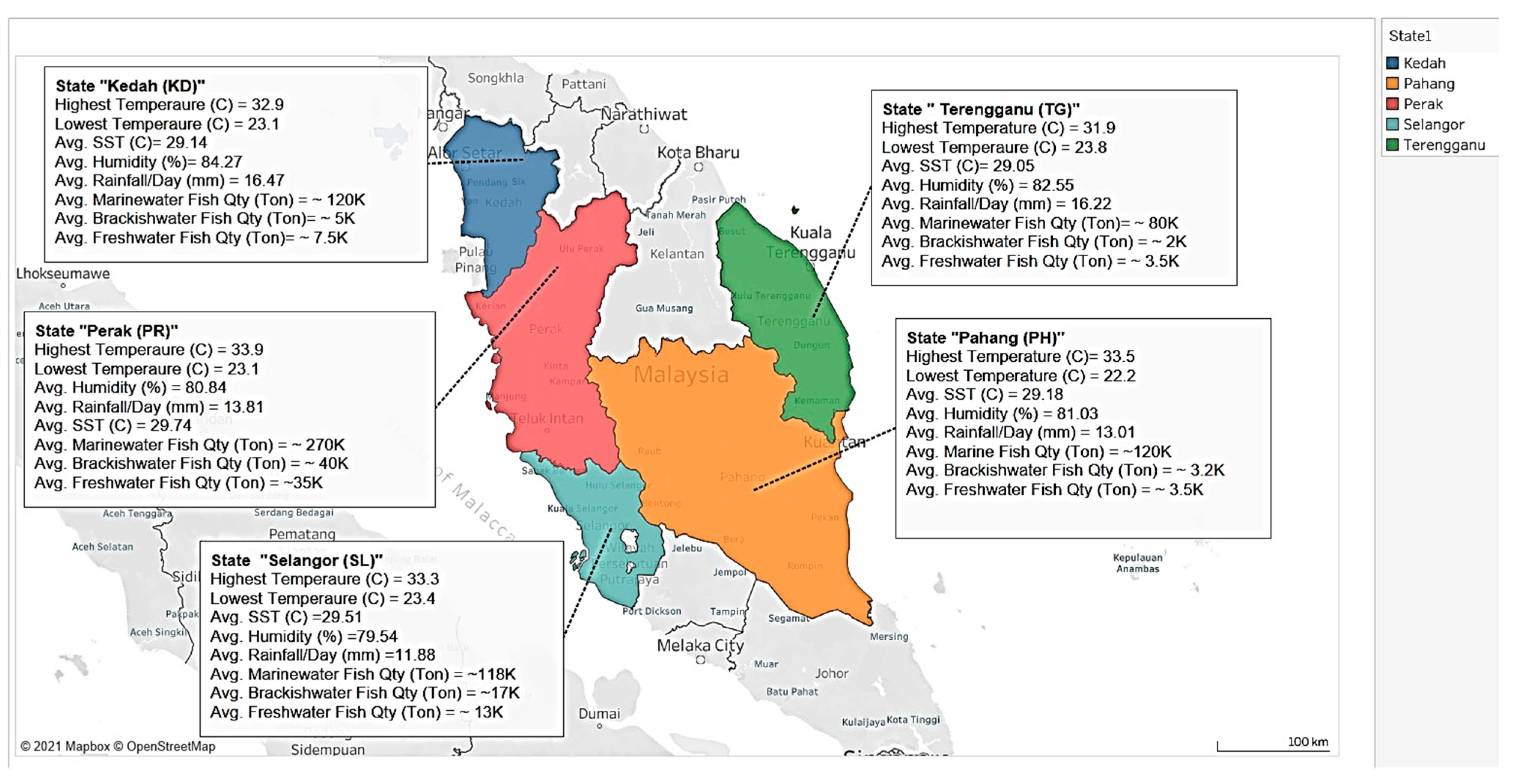
We have selected climatic variables through an extensive literature review. Several climatic variables are recorded as the influencing factors in the fisheries sector, including temperatures, rainfall, salinity, sea level, etc. [35,36,37,38]. The selection of indicators for regional analysis is fraught with constraints, assumptions, and availability of data set. Previous studies demonstrated that rainfall and temperature impact fish landing in the focus country [39]. Similarly, sea surface temperature has been considered an essential indicator for coastal upwelling events influencing fish production reported for the region [40]. Prior studies showed that relative humidity is a significant climatic factor in fisheries studies due to its indirect impact on some environmental stressors [41,42,43]. Therefore, we have collected data of maximum and minimum air temperature, sea surface temperature, rainfall, rainfall duration, and humidity for building models using the different ML approaches. In addition, we considered fish production data for marine landings, brackish water aquaculture, and freshwater aquaculture during data compilation.

2.2. Study Area

Our study site covered the major states of Malaysia named “Selangor”, “Terengganu”, “Kedah”, “Pahang”, and “Perak”. Among these states, Pahang has the largest land area while Selangor has the smallest. All these states border a long coastal area, which helps them to produce more marine fish over the year. We have collected data covering the period from 2000 to 2019 from various organizations in Malaysia that worked with marine water, brackish water, and freshwater fish production. Different states show different fish production quantities and climatic variable statistics, which are shown in Figure 1.

From Figure 1 we can see that the highest temperature was 33.9 °C in Perak, whereas the lowest temperature was 22.2 °C in Terengganu over these 20 years of data. However, the average SST was found as 29 °C for almost all the states. According to Figure 1, it is also observed that Kedah and Terengganu states have a slightly more average rainfall per day (~16 mm) whereas in Pahang and Perak, the value is moderate (~13 mm) and in Selangor, the value is the lowest, i.e., 11.88 mm per day. On the other hand, Kedah recorded the highest humidity at 84.27% whereas Selangor recorded the lowest humidity at 79.54%.

Among all those five major states, the Perak has the highest number of fish landings in marine (~270K tons), fresh (~35K tons), and brackish water (~40K tons). Although the Selangor state has more brackish (~17K tons) and freshwater (~13K tons) fish landings, the marine water fish landings are moderate (~118K tons) compared to other states. The Terengganu state has the lowest fish landings among all states.

2.3. Data Source

We have composed the data set of fish production annual data along with various climatic variable’s statistical data. We have collected the “Rainfall, and humidity” (2000–2019) data from the Department of Statistics Malaysia (DoSM) and ‘‘temperature data’’ (2000–2019); ‘‘sea-surface temperature” (2000–2019) data from the Meteorological Department (MET) of Malaysia. On the other hand, we have obtained the “fish production” (2000–2019) data from the Department of Fisheries Malaysia (DoFM) [44,45,46]. After collecting all the statistical and environmental data, we have combined them into one dataset for five major states of Malaysia. We mapped the individual states into numbers for ML model implementation. At first, we use ordinal encoding to label the states such as Selangor to 1, Terengganu to 2, Pahang to 3, Kedah to 4, and Perak to 0. Then we converted the numbers using a one-hot encoding process to remove biasing of the data. Based on this combined processed dataset from 2000 to 2019 we have analyzed using different ML-based regressions. Additionally, we have used this combined dataset for generating correlation matrices, feature importance scores, and trend line analysis.

2.4. ML-Based Regression

We have applied different ML models such as linear regression (LR), gradient boosting regression (GB), and random forest regression (RF) algorithms based on the feature importance scores. This is because algorithms such as the Tree-based regression technique will help handle data from various measurement scales. These algorithms do not influence outliers and missing values to a fair degree and simplify building rules for predictions about individual cases and complex relationships [34]. As the dataset has different dimensional data so we have chosen RF and GB algorithms. We used the first 17 years of (2000–2016) datasets for model training and the last 3 years of datasets (2017–2019) for testing the accuracy of these models. We have optimized hyperparameters of the ML models based on the cross-validation score. Hyperparameters such as the number of trees in the algorithm, the least number of trials essential to split an internal node, the smallest number of trials required to be at a leaf node, and most importantly, the maximum depth of each tress are adjusted for the RF and GB algorithm. We have assigned the maximum depth of each tree to 7 to ensure the algorithms reduce overfitting of data [38]. We have observed that different ML approaches were suitable for the different datasets. Therefore, we have combined the three ML models in the ensembled VR process and different weight was distributed for a different model as shown in

Table 1. Weight distribution on different ML models in the VR ensemble process.

Fish Production Type	LR	RF	GB
Freshwater	0.05	0.15	0.8
Brackish water	0.8	0.1	0.1
Marine water	0.3	0.35	0.35

. We have applied different combinations and compare the cross-validation scores of the VR model with different combinations of weights. Then we choose the weights which give the highest mean scores in the cross-validation table and the total weight is always equal to 1.

2.5. Error Quality Matrices

We have used Python Scikit learn for the ML implementation and measured different error quality matrices for determining the accuracy of the prediction [31]. Additionally, we have used five error quality matrices to assess the models quantitatively. The quality matrices included the coefficient of determination (R²), root means square error (RMSE), mean absolute error (MAE), and percentage of bias (PBIAS). The different error quality matrices were calculated using the following equations:

$${\mathrm{R}}^2=1-\frac{{{\displaystyle \sum }}_{i=1}^n(F{L}_{measured}-F{L}_{predicted}){ }^2}{{{\displaystyle \sum }}_{i=1}^n{(F{L}_{measured}-{\widehat{FL}}_{measured})}^2}$$

(1)

$$\mathrm{MAPE} =\frac{1}{n}{\displaystyle \sum }_{i=1}^n\left|\frac{F{L}_{measured}-{\widehat{FL}}_{predicted}}{F{L}_{measured}}\times 100\right|$$

(2)

$$\mathrm{MAE} =\frac{1}{n}{\displaystyle \sum }_{i=1}^n|(F{L}_{measured}-F{L}_{predicted})|$$

(3)

$$\mathrm{PBIAS} =\left(\frac{{{\displaystyle \sum }}_{i=1}^n(F{L}_{measured}-F{L}_{predicted})}{{{\displaystyle \sum }}_{i=1}^{n}F{L}_{predicted}}\right)\times 100$$

(4)

where, ${\widehat{FL}}_{measured}$ and ${\widehat{FL}}_{predicted}$ are mean values of predicted and measured fish landing (FL), respectively. In this case, the smaller the values of MAPE means the higher the efficiency of the model. The most common way to measure the performance is the R² value which is between 0 and 1 [40]. We have compared the predicted fish production values with the observed values for measuring the efficiency of the ML model output.

3. Results

3.1. Correlation Matrix

A correlation matrix is needed to describe the relationships between the climatic variables and locations, which is illustrated in

Table 2. Correlation between the climatic variables and locations in Malaysia.

	State	Rainfall	RF Duration	Max Temp	Min Temp	SST	Humidity
State	1
Rainfall	0.387	1
RF Duration	0.428	0.613	1
Max Temp	0.448	−0.171	0.159	1
Min Temp	−0.358	−0.238	−0.236	0.275	1
SST	0.100	−0.109	0.089	0.264	−0.037	1
Humidity	0.235	0.411	0.230	−0.495	−0.473	−0.322	1

.

This research calculated the impact of climatic variables using the Pearson Correlation Index (PCI), where the relationship is defined according to the size of the coefficient (0.9–1, very high; 0.7–0.89, high; 0.5–0.69, moderate; 0.26–0.49, weak; 0–0.25, very weak) [47]. According to the PCI matrix, one parameter’s negative value is found in inverse relation to another parameter. If a parameter has a decreasing value, then another parameter value has an increasing value. For example, in Table 2, a moderate positive correlation is observed between rainfall and rainfall duration (r = 0.61; p < 0.01). This relation implied that an increase in rainfall duration is related to the total amount of rainfall. Additionally, rainfall and rainfall duration data are positively related with states, which means that state-wise rainfall and rainfall duration has a weak impact on fish landings. On the other hand, it has been observed from the correlation data as shown in Table 2 that, state-wise maximum temperature also has a weak positive correlation on the state (r = 0.44; p < 0.01). However, it is observed from Table 2 that climatic variable humidity has a weak positive correlation with rainfall (r = 0.41; p < 0.01). On the other hand, humidity data has weak negative correlation with maximum temperature (r = −0.49; p < 0.01) and minimum temperature (r = −0.47; p < 0.01). This negative correlation implies that if the humidity of any state increases then the maximum or minimum temperature could decrease of that state. Generally, SST rises due to the absorption of more heat by the sea, which changes the ocean circulation patterns [48]. Moreover, the duration of rainfall, temperature variability, and humidity data may affect the fish landings [49]. As there is no significant correlation observed among the climatic variables and location, so for further investigation, feature importance parameters have taken into consideration to analyze the fish landing datasets for five major states of Malaysia. Here, correlation analysis has been done among the three types of water and climatic variables, which is shown in

Table 3. Correlation between the climatic variables and different types of fish landings in Malaysia.

	Rainfall	RF Duration	Max Temp	Min Temp	SST	Humidity
Marine fish	0.155	0.478	0.515	−0.129	0.304	−0.165
Brackish water fish	0.045	0.391	0.401	−0.090	0.303	−0.110
Freshwater fish	0.094	0.361	0.358	−0.076	0.227	−0.201

.

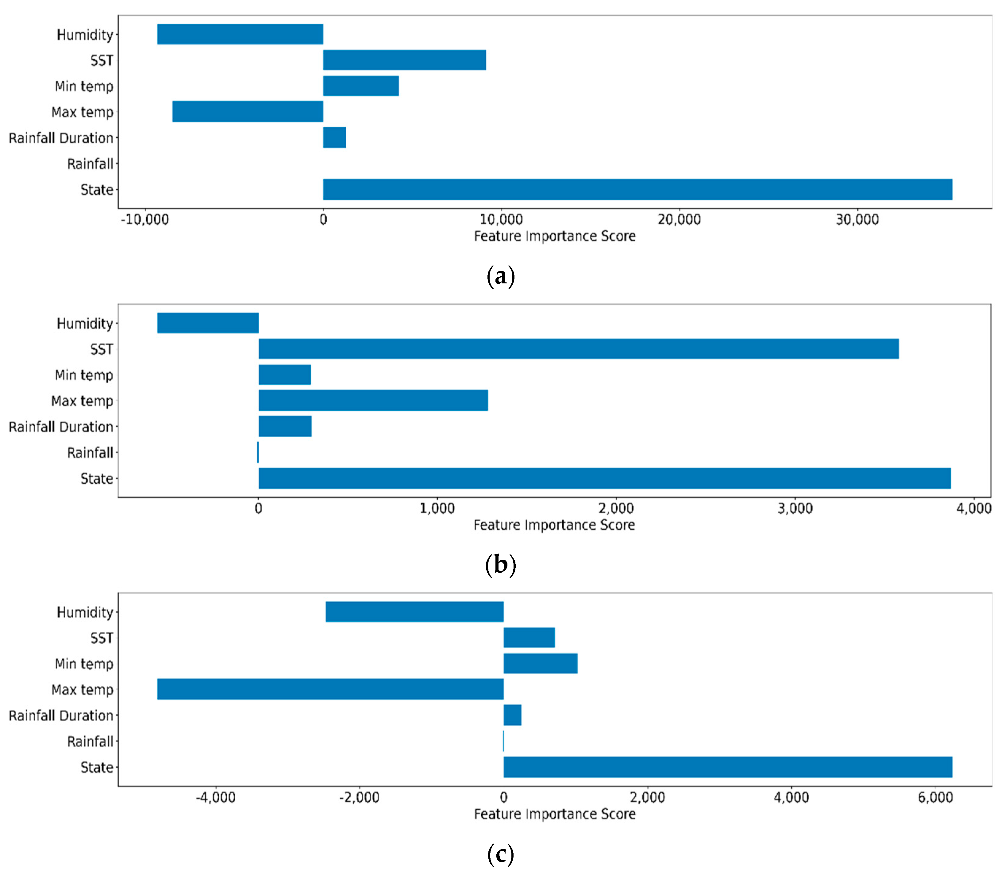
3.2. Feature Importance Analysis

According to the correlation table, finding the important climatic variables is quite limited, which are affecting the catchment of different fishes. Therefore, feature importance analysis for predicting the various ML models has been included. Based on the dataset, ML models, dimension reduction, selection of climatic variables feature is necessary to improve the efficiency and effectiveness of any predictive model. Figure 2 shows the feature importance graph of climatic variables, which has been taken into consideration for marine water, brackish water, and freshwater fish productions. The ML-based feature importance model given an importance score for each variable where the larger score implies that the variable is more important [50]. The figure shows that no matter what type of fish we considered, the location always plays the most important role. Therefore, the ML model also included the states as one of the major dependent variables for predicting fish productions in Malaysia. Moreover, from Figure 2a,b, it is found that, for marine water, rainfall, rainfall duration and minimum temperature are found to be less significant. Therefore, these climatic variables were not used in different ML models. Instead, Figure 2c shows that for freshwater fish landings, rainfall, rainfall duration and SST were found less significant. Nevertheless, from Figure 2, it is obvious that humidity is negatively scored in feature importance analysis for all three categories of fish productions, which is also identical to the correlation table (Table 2). However, SST is identified as an important feature for both marine water and brackish water, which should be taken into consideration during prediction modeling.

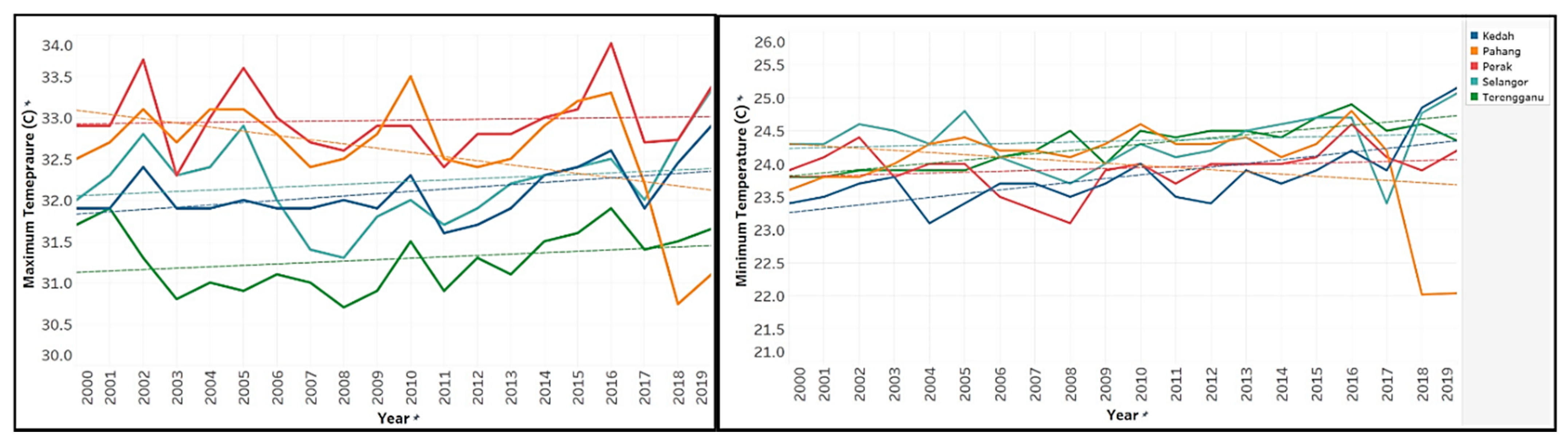
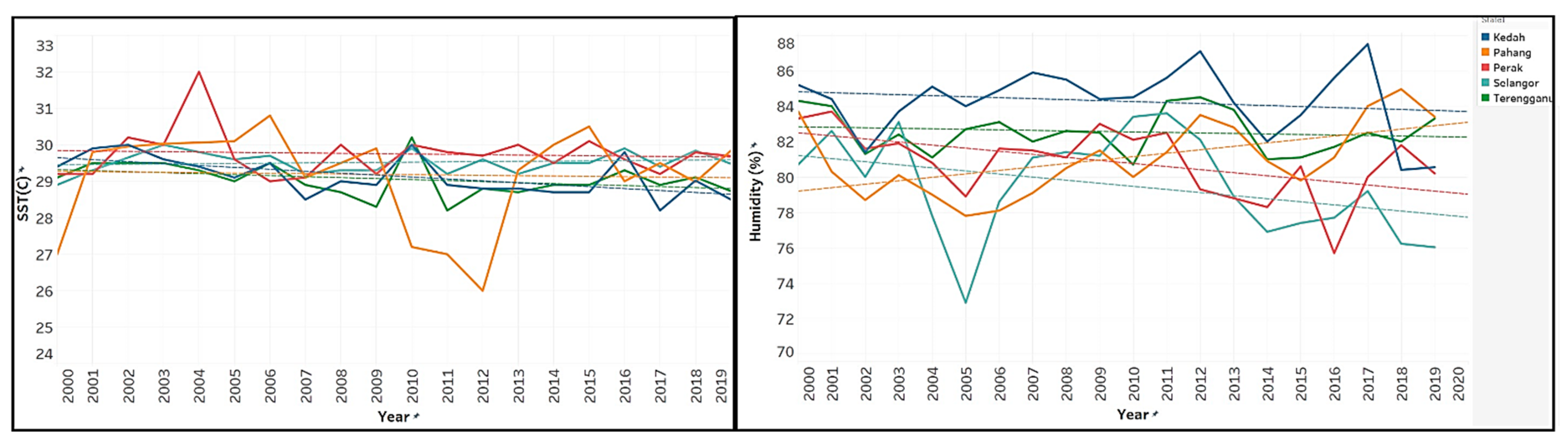
3.3. Trend Line Analysis

Several climatic variables have been considered such as maximum and minimum air temperature, SST, humidity for building different models. Using the LR model, Figure 3 shows the trend line of maximum and minimum air temperatures in Malaysia’s major five states from 2000 to 2019. We can observe an upward trend in the maximum temperature as shown in Figure 3 except the Pahang state, which is showing a downward trend. In addition, we observed a sharp fall in temperature in the year 2017 except the Pahang state which rapidly falls in the year 2018. The temperature started to rise again in 2019. It was also observed that there was a slightly increasing trend line in the minimum temperature over the period (2000 to 2019). We can see a sharp fall in minimum temperature in the case of Pahang state from 2017 to 2018.

Figure 4 shows the trendline of humidity and SST in five major states of Malaysia over the period (2000 to 2019). We found that humidity is showing a descending trend line in four states of Malaysia except for Pahang which is in an upward trend from 2000 to 2019. The SST started to fall from 30 °C in 2009 to 26 °C in 2012. Again in 2012, SST shows the inclining trend. Overall, the SST trend line indicated that the impact of a large period dataset on the variability of SST changes very little (except for the Pahang state), which can be less noticeable. The lowest average humid day was recorded in 2005 in Selangor (72.9%), whereas, in 2017, the highest humidity was recorded in Kedah with 87.5%.

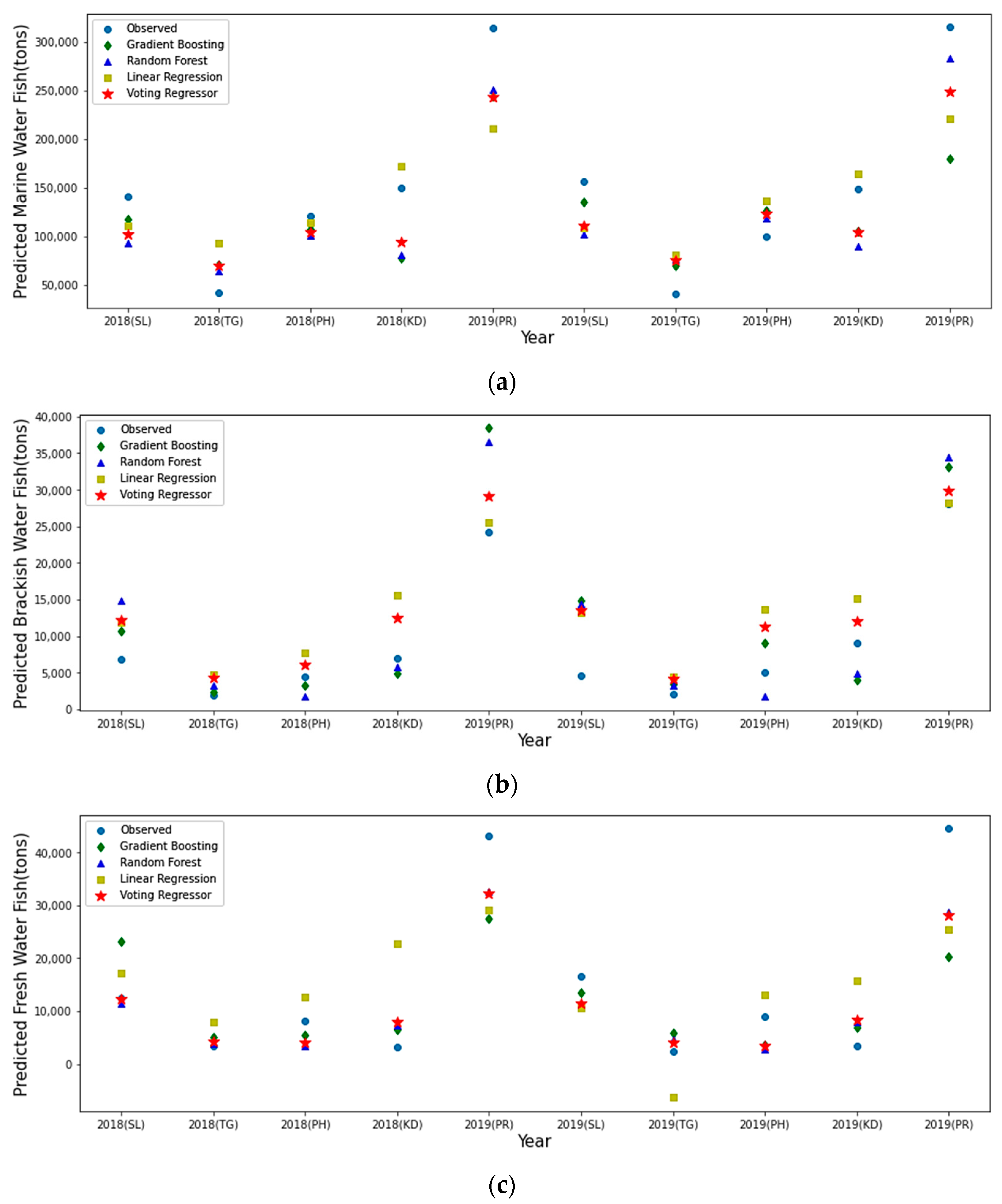
3.4. ML-Based Prediction

Four ML-based prediction models, known as the LR, GB, RF, and VR models are implemented to predict marine, fresh, and brackish water fish landing (in tons). After implementing the four ML algorithms, the comparison graph is shown in Figure 5. The VR ensembled ML model shows a better result compared to the individual ML model. In Figure 5, the X-axis is showing all five states’ output for 2018 and 2019. The Y-axis shows the comparison of the predicted values based on the 4 ML models. According to Figure 5, we found that the VR model output is closest compared to the observed dataset. Additionally, this figure indicates that the linear regression has a high bias, whereas RF and GB have comparatively improved prediction results with low bias. Moreover, in 2019, data for freshwater we have found that the LR has given negative values, proving that the LR model will produce a low prediction accuracy.

4. Discussion

By comparing all the figures above, we can see that a single ML model does not give the best prediction every time. Therefore, we have applied the VR technique to ensemble the three different ML models. This VR model is used to average multiple ML models with customized weight values improving the accuracy.

Table 4. Comparison study of four regression models.

	Linear (LR)	Gradient Boost	Random Forest	Voting
R2	0.64	0.74	0.71	0.75	Marine Water Fish
MAPE	0.416	0.384	0.414	0.385
MAE	45,686.619	43,414.895	45,805.751	42,160.472
PBIAS	0.076107	0.148685	0.172827	0.135361
R2	0.38	0.81	0.79	0.81	Freshwater Fish
MAPE	1.408	0.661	0.579	0.683
MAE	8966.13	5354.083	5428.294	5517.096
PBIAS	0.046812	0.192765	0.213581	0.188589
R2	0.44	−0.57	−0.073	0.55	Brackish Water Fish
MAPE	1.189	1.032	0.71	1.072
MAE	5591.54	7652.332	5768.358	5412.247
PBIAS	−0.585898	−0.467072	−0.335735	−0.548999

describes the comparative study of four regression models used in this research with the error quality matrix for marine water, brackish water, and freshwater fish production prediction in different ML models.

The ML model’s prediction performance is measured in terms of four error objective functions, which are R², MAPE, MAE, and PBIAS as we are dealing with time-series data.

MAPE indicates how much error in prediction is compared to the measured value in the series. Additionally, MAPE is used for comparison of the precision of the same or different methods in two different series and measure the accuracy of the estimated value of the model expressed in terms of the absolute percentage error average [41]. In this case, the smaller the values of MAPE means the higher the efficiency of the model. From Table 4 MAPE values of LR, GB, RF, and VR are 0.41, 0.38, 0.41, 0.38, respectively for marine water fish. These values reflect that GB and VR models showed more efficiency among these models. On the other hand, for freshwater and brackish water fish landings, MAPE values are found quite high compared to marine water fish landings. However, MAPE results can be skewed if there are zero or close to zero values in the dataset, which is a disadvantage of this error function [42].

Generally, the optimal value of error indices MAE is zero and the smaller are the values, the more accurate are the simulations [42]. From Table 4, it is found that the MAE value of the VR model is the smallest at 42,160.472, which proved that, among these ML models ensembled VR model is more accurate for predicting the marine water fish landings. Similarly, in brackish water fish landings, the MAE value of the VR model is the smallest at 5412.247, which also showed the best accuracy among other predictive models. However, for freshwater fish landings, the GB model generated the best accuracy with the MAE smallest value of 5354.083. On the other hand, PBIAS measures the average tendency of the simulated values to be larger or smaller than their observed ones. Positive values indicate model underestimation bias, and negative values indicate model overestimation bias [51]. From Table 4, it is observed that both marine water and freshwater fish landing’s best accuracy is obtained from LR modeling, which is 0.076 and 0.046, respectively. However, for brackish water fish landings, negative values are observed.

Most importantly, researchers measure the ML model performance in terms of the R² values. In the case of marine fish, the R² values of LR, GB, RF are 0.64, 0.74, and 0.71, respectively. However, when the VR technique is applied to ensemble these three ML models, the R² value became 0.75, which is higher inaccuracy. On the other hand, for freshwater fish, the R² values of LR, GB, RF are 0.38, 0.81, and 0.79, respectively. Nevertheless, after applying the ensemble approach, the VR value is found at 0.81, which is equivalent to the highest value obtained by an individual model. The VR model boosts the performance in the brackish water fish landing prediction. The R² values of LR, GB, RF are 0.44, −0.57, and −0.073, respectively. However, when the VR ensemble is applied, the accuracy of the prediction is improved and increased to 0.55. Hence, based on the R² values, the VR-based ensembled ML model is the best ML-based prediction model for fish landings in Malaysia.

Based on the score achieved in feature importance implementation, it is evident that climatic variables have an impact on marine water, brackish water, and freshwater fish production. The ML model performance also greatly depends on the variables that have more predicting power. We have determined this predictive power of individual climatic variables using the feature importance method and found that rainfall (rf) has the least impact among all variables and temperature has more influences on fish production. We have improved the ML model performance by doing such pre-processing of the data.

The fisheries industry is an important sector in sustaining the economy of Malaysia as changes in climatic variables may alter fish production or overfishing. Therefore, the prediction of annual fish productions in Malaysia is significant for sustainable development along with the continuous fish catch. In this regard, this research has implemented the feature importance method to determine the impact score of the climatic variables over different types of fish landings. Based on the score, the annual climatic data are considered and divided into training and testing set to predict the annual fish landings of all five major states. These variables have been considered for building models using the different ML approaches LR, RF, GB, and ensembled VR. In addition, fish production data from 2000 to 2019 for three different types of water such as marine, brackish, and freshwater is considered for developing these ML models. Generally, it is stated that changes in fish landings are consistent with the temperature and higher temperature means higher fish productions [52]. In addition, fish landings may reduce before temperature decreases, which reflects that climatic variable air temperature may influence the total fish landings by altering the habitat availability and quality.

We see in this study that when the R², MAPE, MAE, and PBIAS values were used for selecting the best model, the ML models emerged as the better models in predicting fish production in Malaysia. However, if the R² value is selected as the forecast accuracy measurement for model selection, then the ML models can be used as the alternative models in predicting the demersal marine fish and freshwater fish production in Malaysia. In this research, the dataset contained all five major states in both the validation and testing phases. Thus, ML models used in this research can predict fish production in five major states of Malaysia. The fishery industry’s decision-makers usually plan according to the fishing market’s resource requirement, which is highly dependent on the accurate forecasts of one or two years of fish landings in advance [53]. Therefore, this predictive model can be a valuable component to build future decision support systems (DSS) for Malaysia’s fishing industry.

5. Conclusions

Machine learning algorithms are efficient to solve complex time series data and have been widely used in the environmental field. Applied ML models sometimes faced a problem with many potential inputs but limited datasets are available. Here, we applied a hybrid approach, which included feature importance measures, and an ML model. We have implemented these models to extract valuable and meaningful information from the selected climatic variables and to explore the impacts on marine fish, brackish water aquaculture, and freshwater aquaculture production. We have used the past 20 years of data from five major states of Malaysia for generating the ML models. A performance matrix evaluates the ML model performance in terms of 4 error objective functions. ML-based feature importance method first identified the more predictor values. Based on those values, we have chosen 3 climatic variables and the location as input of the ML models. We have implemented 3 ML models and one ensembled approach (VR). The results show that the ensembled VR value is found 0.75, 0.81, 0.55 for marine water, freshwater, and brackish water, respectively, which is better compared to the single ML model. Hence, we can conclude that instead of one ML model, an ensemble approach outperforms the other ML model in predicting all three types of fish production (in tons). This research provides an ML model-based framework that delivers a reliable and accurate estimation of fish production in the study area. This ensembled ML approach with the feature importance method will be a valuable tool to predict fish data and help Malaysian stakeholders and policymakers to implement such tools to help guide fish production strategies in Malaysia.

References

1. Hicks, C.C.; Cohen, P.J.; Graham, N.A.; Nash, K.L.; Allison, E.H.; D’Lima, C.; MacNeil, M.A. Harnessing global fisheries to tackle micronutrient deficiencies. Nature 2019, 574, 95–98. [Google Scholar] [CrossRef] [Green Version]
2. Srinivasan, U.T.; Cheung, W.W.; Watson, R.; Sumaila, U.R. Food security implications of global marine catch losses due to overfishing. J. Bioecon. 2010, 12, 183–200. [Google Scholar] [CrossRef]
3. Sumaila, U.R.; Cheung, W.W. Boom or Bust: The Future of Fish in the South China Sea; Fisheries Center, University of British Columbia: Vancouver, BC, Canada, 2015. [Google Scholar]
4. Haghshenas, E.; Gholamalifard, M.; Mahmoudi, N.; Kutser, T. Developing a GIS-based decision rule for sustainable marine aquaculture site selection: An application of the ordered weighted average procedure. Sustainability 2021, 13, 2672. [Google Scholar] [CrossRef]
5. Ahmad, A.; Abdullah, S.R.S.; Hasan, H.A.; Othman, A.R.; Ismail, N.I. Aquaculture industry: Supply and demand, best practices, effluent and its current issues and treatment technology. J. Environ. Manag. 2021, 287, 112271. [Google Scholar] [CrossRef]
6. Jeevanaraj, P.; Hashim, Z.; Elias, S.M.; Aris, A.Z. Risk of dietary mercury exposure via marine fish ingestion: Assessment among potential mothers in Malaysia. Expo. Health 2019, 11, 227–236. [Google Scholar] [CrossRef]
7. Norimah, A.K., Jr.; Safiah, M.; Jamal, K.; Haslinda, S.; Zuhaida, H.; Rohida, S.; Fatimah, S.; Norazlin, S.; Poh, B.K.; Kandiah, M.; et al. Food consumption patterns: Findings from the Malaysian Adult Nutrition Survey (MANS). Malays. J. Nutr. 2008, 14, 25–39. [Google Scholar]
8. Abu, T.; Mohammad, I.; Mohamad, S.I.; Sharum, Y. Status of demersal fishery resources of Malaysia. Assess. Manag. Future Direct. Coastal Fish. Asian Ctries. 2003, 67, 83–136. [Google Scholar]
9. Biusing, R. Assessment of Coastal Fisheries in the Malaysian-Sabah portion of the Sulu-Sulawesi Marine Ecoregion (SSME); Buhavan InfoTech: Sabah, Malaysia, 2001. [Google Scholar]
10. Kathijotes, N.; Alam, L.; Kontou, A. Aquaculture, coastal pollution and the environment. In Aquaculture Ecosystems: Adaptability and Sustainability, 1st ed.; Mustafa, S., Shapawi, R., Eds.; John Wiley & Sons, Ltd: Hoboken, NJ, USA, 2015; Chapter 5, pp. 139–163. [Google Scholar]
11. Department of Statistics, Malaysia. Available online: https://www.dosm.gov.my/v1/index.php/index.php?r=column/pdfPrev&id=K3I2eG9kUlVBOEhoOHdITGtrWFNlZz09 (accessed on 7 August 2017).
12. Von Goh, E. The Status of Fish in Malaysian Diets and Potential Barriers to Increasing Consumption of Farmed Species. Ph.D. Thesis, University of Nottingham, Semenyih, Malaysia, 2018. [Google Scholar]
13. Yusoff, A. Status of resource management and aquaculture in Malaysia. In Resource Enhancement and Sustainable Aquaculture Practices in Southeast Asia: Challenges in Responsible Production of Aquatic Species: Proceedings of the International Workshop on Resource Enhancement and Sustainable Aquaculture Practices in Southeast Asia 2014 (RESA); Aquaculture Department, Southeast Asian Fisheries Development Center: Tigbauan, Philippines, 2015; pp. 53–65. [Google Scholar]
14. Solaymani, S. Impacts of climate change on food security and agriculture sector in Malaysia. Environ. Dev. Sustain. 2018, 20, 1575–1596. [Google Scholar] [CrossRef]
15. Ahmed, N.; Thompson, S.; Glaser, M. Global aquaculture productivity, environmental sustainability, and climate change adaptability. Environ. Manag. 2019, 63, 159–172. [Google Scholar] [CrossRef]
16. Brander, K.M. Global fish production and climate change. Proc. Natl. Acad. Sci. USA 2007, 104, 19709–19714. [Google Scholar] [CrossRef] [Green Version]
17. De Silva, S.S.; Soto, D. Climate change and aquaculture: Potential impacts, adaptation and mitigation. In Climate Change Implications for Fisheries and Aquaculture: Overview of Current Scientific Knowledge; FAO Fisheries and Aquaculture Technical Paper; FAO Fisheries and Aquaculture: Rome, Italy, 2009; Volume 530, pp. 151–212. [Google Scholar]
18. Hanjra, M.A.; Qureshi, M.E. Global water crisis and future food security in an era of climate change. Food Policy 2010, 35, 365–377. [Google Scholar] [CrossRef]
19. Turral, H.; Burke, J.; Faurès, J.M. Climate Change, Water and Food Security; No. 36; Food and Agriculture Organization of the United Nations (FAO): Rome, Italy, 2011. [Google Scholar]
20. Food and Agriculture Organization of the United Nations. Our Actions Are Our Future: A #ZeroHunger World by 2030 Is Possible; FAO: Rome, Italy, 2018. [Google Scholar]
21. Govindan, K.; Khodaverdi, R.; Jafarian, A. A fuzzy multi criteria approach for measuring sustainability performance of a supplier based on triple bottom line approach. J. Clean. Prod. 2013, 47, 345–354. [Google Scholar] [CrossRef]
22. Coro, G.; Large, S.; Magliozzi, C.; Pagano, P. Analyzing and forecasting fisheries time series: Purse seine in Indian Ocean as a case study. ICES J. Mar. Sci. 2016, 73, 2552–2571. [Google Scholar]
23. Yadav, V.K.; Jahageerdar, S.; Adinarayana, J. Modelling framework to study the influence of environmental variables for forecasting the quarterly landing of total fish catch and catch of small major pelagic fish of north-west Maharashtra coast of India. Natl. Acad. Sci. Lett. 2020, 43, 515–518. [Google Scholar] [CrossRef]
24. Paul, R.K.; Sinha, K. Forecasting crop yield: ARIMAX and NARX model. RASHI 2016, 1, 77–85. [Google Scholar]
25. Anuja, A.; Yadav, V.K.; Bharti, V.S.; Kumar, N.R. Trends in marine fish production in Tamil Nadu using regression and autoregressive integrated moving average (ARIMA) model. J. Appl. Nat. Sci. 2017, 9, 653–657. [Google Scholar] [CrossRef] [Green Version]
26. Marufuzzaman, M.; Tumbraegel, T.; Rahman, L.F.; Sidek, L.M. A machine learning approach to predict the activity of smart home inhabitant. J. Ambient Intell. Smart Environ. 2021, 13, 271–283. [Google Scholar] [CrossRef]
27. Majid, R.; Mir, S.A. Advances in statistical forecasting methods: An overview. Econ. Aff. 2018, 63, 815–831. [Google Scholar] [CrossRef]
28. Haupt, S.E.; Cowie, J.; Linden, S.; McCandless, T.; Kosovic, B.; Alessandrini, S. Machine learning for applied weather prediction. In Proceedings of the 2018 IEEE 14th International Conference on e-Science, Amsterdam, The Netherlands, 29 October–1 November 2018; pp. 276–277. [Google Scholar]
29. Stefanovič, P.; Štrimaitis, R.; Kurasova, O. Prediction of flight time deviation for lithuanian airports using supervised machine learning model. Comput. Intell. Neurosci. 2020, 2020, 10. [Google Scholar] [CrossRef]
30. Ahmed, A.N.; Othman, F.B.; Afan, H.A.; Ibrahim, R.K.; Fai, C.M.; Hossain, M.S.; Ehteram, M.; Elshafie, A. Machine learning methods for better water quality prediction. J. Hydrol. 2019, 578, 124084. [Google Scholar] [CrossRef]
31. Rastrollo-Guerrero, J.L.; Gómez-Pulido, J.A.; Durán-Domínguez, A. Analysing and predicting students’ performance by means of machine learning: A review. Appl. Sci. 2020, 10, 1042. [Google Scholar] [CrossRef] [Green Version]
32. Knudby, A.; LeDrew, E.; Brenning, A. Predictive mapping of reef fish species richness, diversity and biomass in Zanzibar using IKONOS imagery and machine-learning techniques. Remote Sens. Environ. 2010, 114, 1230–1241. [Google Scholar] [CrossRef]
33. Alam, L.; Mokhtar, M.; Ta, G.C.; Halim, S.A.; Ahmed, M.F. Review on regional impact of climate change on fisheries sector. Nov. J. 2017, 4, 1–5. [Google Scholar]
34. Tehrany, M.S.; Pradhan, B.; Jebur, M.N. Spatial prediction of flood susceptible areas using rule-based decision tree (DT) and a novel ensemble bivariate and multivariate statistical models in GIS. J. Hydrol. 2013, 504, 69–79. [Google Scholar] [CrossRef]
35. Pal, M.; Mather, P.M. An assessment of the effectiveness of decision tree methods for land cover classification. Remote. Sens. Environ. 2003, 86, 554–565. [Google Scholar] [CrossRef]
36. Kausar, R.; Salim, M. Effect of water temperature on the growth performance and feed conversion ratio of Labeo rohita. Pak. Vet. J. 2006, 26, 105–108. [Google Scholar]
37. Thakur, K.K.; Vanderstichel, R.; Barrell, J.; Stryhn, H.; Patanasatienkul, T.; Revie, C.W. Comparison of remotely-sensed sea surface temperature and salinity products with in situ measurements from British Columbia, Canada. Front. Mar. Sci. 2018, 5, 121. [Google Scholar] [CrossRef] [Green Version]
38. Brame, M. Avoiding overfitting of decision trees. In Principles of Data Mining; Springer: Berlin/Heidelberg, Germany, 2007; pp. 119–134. [Google Scholar]
39. Pedregosa, F.; Varoquaux, G.; Gramfort, A.; Michel, V.; Thirion, B.; Grisel, O.; Blondel, M.; Prettenhofer, P.; Weiss, R.; Dubourg, V.; et al. Scikit-learn: Machine learning in Python. J. Mach. Learn. Res. 2011, 12, 2825–2830. [Google Scholar]
40. Bui, D.T.; Khosravi, K.; Tiefenbacher, J.; Nguyen, H.; Kazakis, N. Improving prediction of water quality indices using novel hybrid machine-learning algorithms. Sci. Total Environ. 2020, 721, 137612. [Google Scholar] [CrossRef]
41. Prayudani, S.; Hizriadi, A.; Lase, Y.Y.; Fatmi, Y. Analysis accuracy of forecasting measurement technique on random K-nearest neighbor (RKNN) using MAPE and MSE. J. Phys. Conf. Ser. 2019, 1361, 012089. [Google Scholar] [CrossRef]
42. Hyndman, R.J.; Khandakar, Y. Automatic Time Series for Forecasting: The Forecast Package for R; Department of Econometrics and Business Statistics, Monash University: Melbourne, VIC, Australia, 2007. [Google Scholar]
43. Curceac, S.; Atkinson, P.M.; Milne, A.; Wu, L.; Harris, P. Adjusting for conditional bias in-process model simulations of hydrological extremes: An experiment using the North Wyke Farm Platform. Front. Artif. Intell. 2020, 3, 82. [Google Scholar] [CrossRef] [PubMed]
44. Department of Statistics Malaysia. Available online: https://www.dosm.gov.my/v1/index.php/index.php?r=column3/accordion&menu_id=amZNeW9vTXRydTFwTXAxSmdDL1J4dz09 (accessed on 15 July 2021).
45. Malaysian Meteorological Department. Available online: https://www.met.gov.my/info/perkhidmatan?lang=en (accessed on 21 July 2021).
46. Department of Fisheries Malaysia. Available online: https://www.dof.gov.my/index.php/pages/view/82 (accessed on 21 July 2021).
47. Geng, X.; Zhang, D.; Li, C.; Li, Y.; Huang, J.; Wang, X. Application and Comparison of Multiple Models on Agricultural Sustainability Assessments: A Case Study of the Yangtze River Delta Urban Agglomeration, China. Sustainability 2021, 13, 121. [Google Scholar] [CrossRef]
48. Goreau, T.J.; Hayes, R.L.; McAlllister, D. Regional patterns of sea surface temperature rise: Implications for global ocean circulation change and the future of coral reefs and fisheries. World Resour. Rev. 2005, 17, 350–370. [Google Scholar]
49. Wall, R.; Howard, J.J.; Bindu, J. The seasonal abundance of blowflies infesting drying fish in south-west India. J. Appl. Ecol. 2001, 38, 339–348. [Google Scholar] [CrossRef]
50. Zien, A.; Krämer, N.; Sonnenburg, S.; Rätsch, G. The feature importance ranking measure. In Proceedings of the Joint European Conference on Machine Learning and Knowledge Discovery in Databases, Bled, Slovenia, 6–9 September 2009; Springer: Berlin/Heidelberg, Germany, 2009; pp. 694–709. [Google Scholar]
51. Gupta, H.V.; Sorooshian, S.; Yapo, P.O. Status of automatic calibration for hydrologic models: Comparison with multilevel expert calibration. J. Hydrol. Eng. 1999, 4, 135–143. [Google Scholar] [CrossRef]
52. Cochrane, K.; De Young, C.; Soto, D.; Bahri, T. (Eds.) Climate change implications for fisheries and aquaculture: Overview of current scientific knowledge. In Food and Agriculture Organization of the United Nations Fisheries and Aquaculture Technical Paper; No. 530; FAO: Rome, Italy, 2009. [Google Scholar]
53. Felthoven, R.G.; Paul, C.J.M. Directions for productivity measurement in fisheries. Mar. Policy 2004, 28, 161–169. [Google Scholar] [CrossRef]
Figure 1. Comparison of different climatic variables and the average annual fish landings in five major states of Malaysia.
Sustainability 13 09124 g001
Figure 2. Feature importance analysis for (a) marine water, (b) brackish water and (c) freshwater fish landing dataset.
Sustainability 13 09124 g002
Figure 3. Maximum/minimum temperature data trends of five states over the period 2000 to 2019.
Sustainability 13 09124 g003
Figure 4. SST and humidity data trends of five states over the period 2000 to 2019.
Sustainability 13 09124 g004
Figure 5. Comparison of different ML predictions for (a) marine water (b) brackish water (c) freshwater fish landings using the testing dataset.
Sustainability 13 09124 g005