
Identification of a Set of Variables for the Classification of Páramo Soils Using a Nonparametric Model, Remote Sensing, and Organic Carbon


Abstract
:1. Introduction
2. Materials and Methods
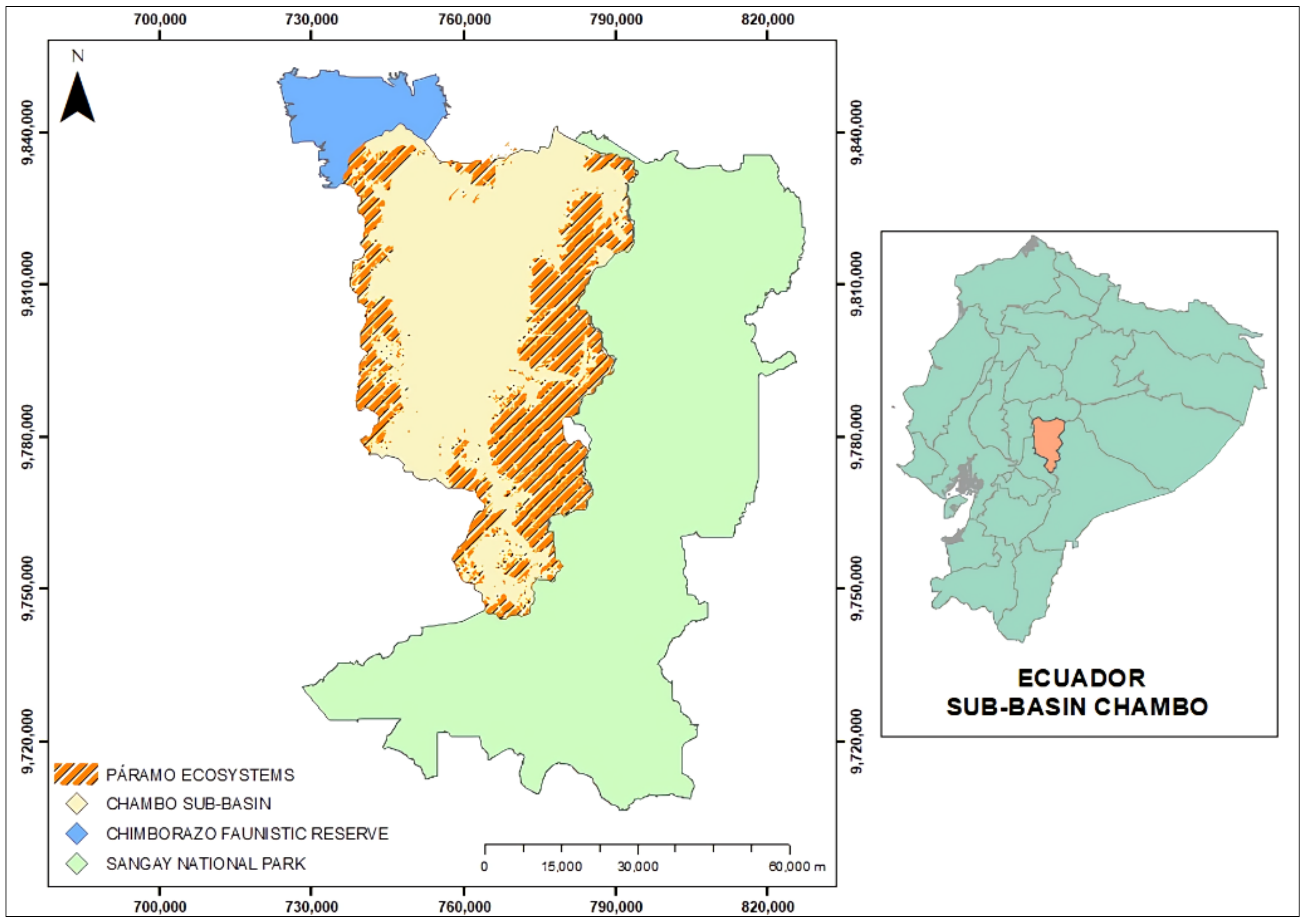
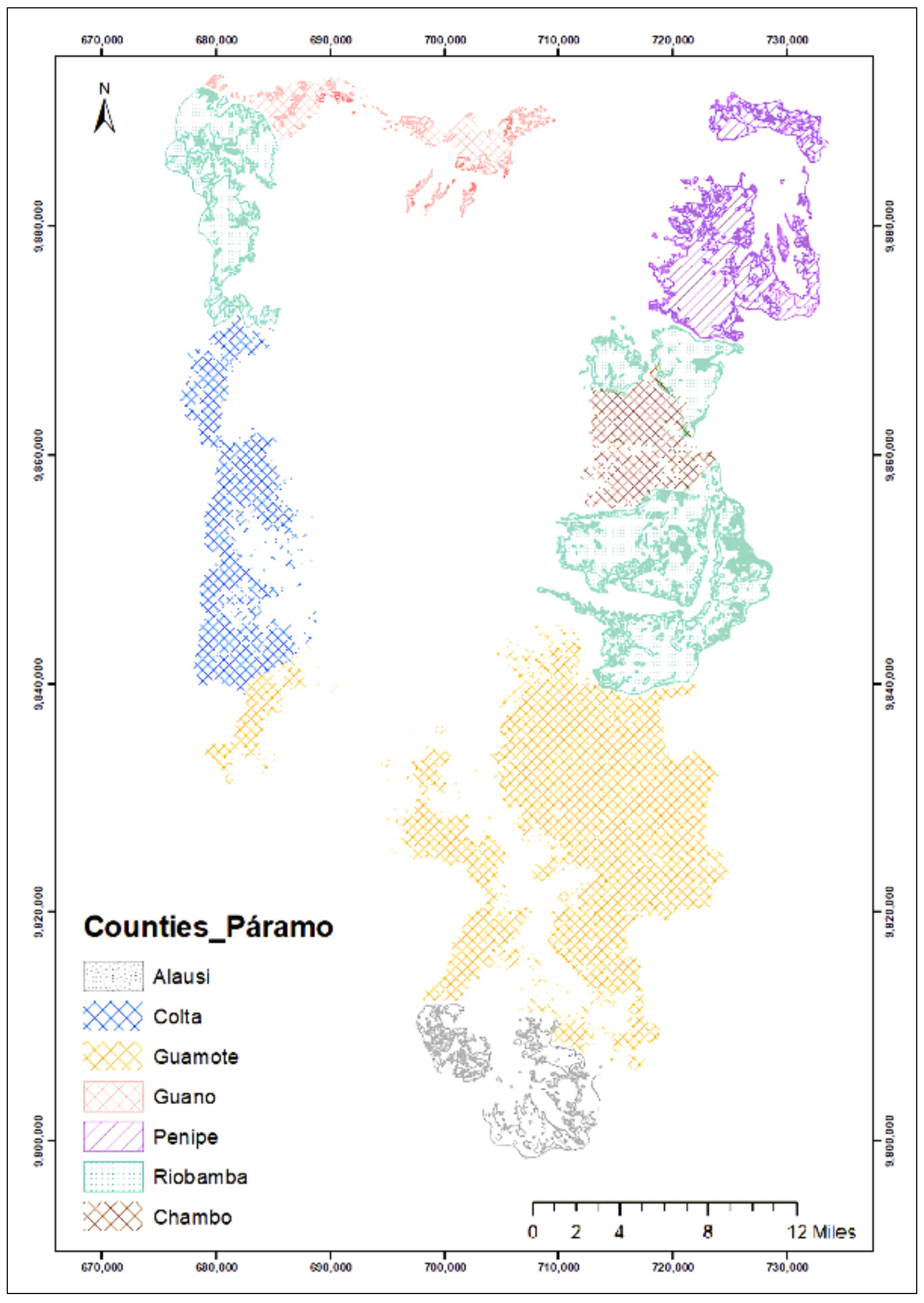
2.1. Study Area
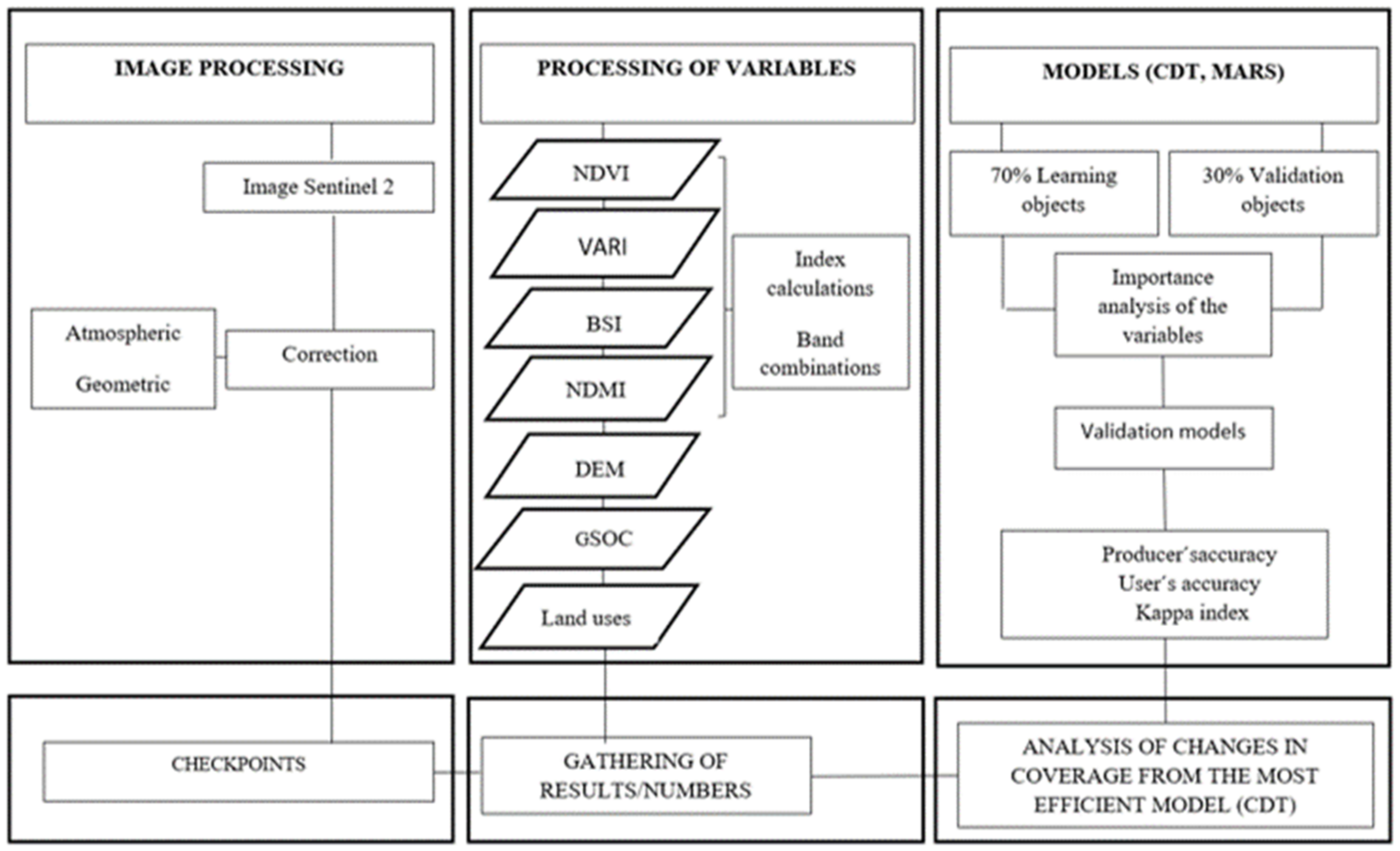
2.2. Work Flow
2.3. Satellite Images
2.4. Image Processing
2.5. Checkpoints
2.6. Variables
2.7. Extraction of Values
2.8. Fitting of Data in the Supervised Learning Model
2.9. Nonparametric Methods of Classification
2.9.1. CART Decision Tree (CDT)
2.9.2. Multivariate Adaptive Regression Splines (MARS)
3. Results and Discussion
3.1. Spearman’s Rank Correlation Matrix—Order Matrix
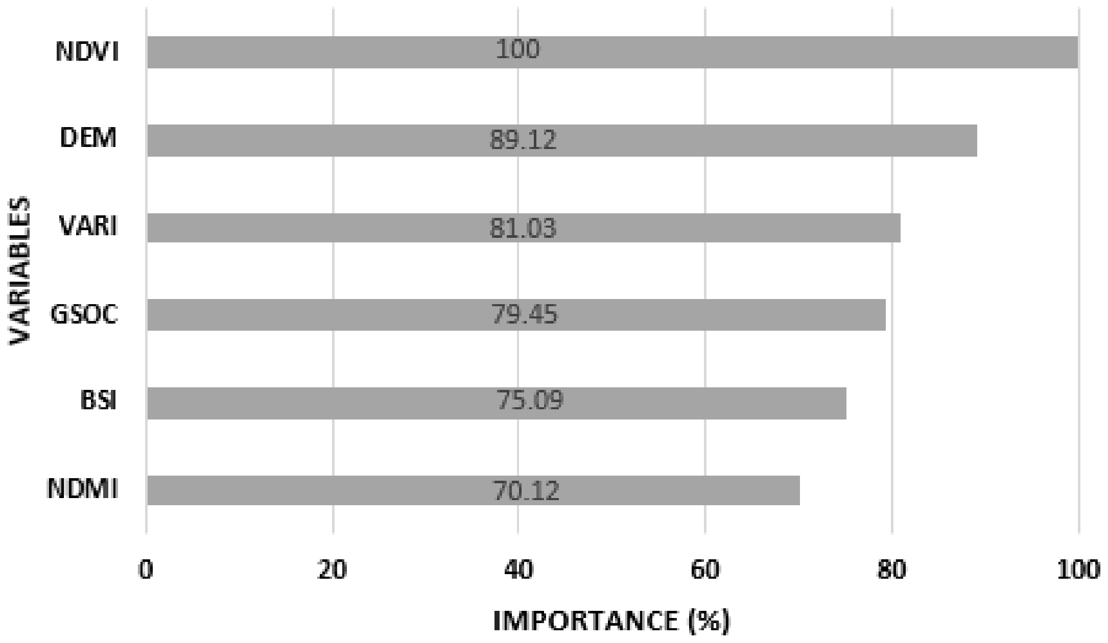
3.2. Analysis of the Variables of Importance
3.3. Precision Assessment of Nonparametric Models
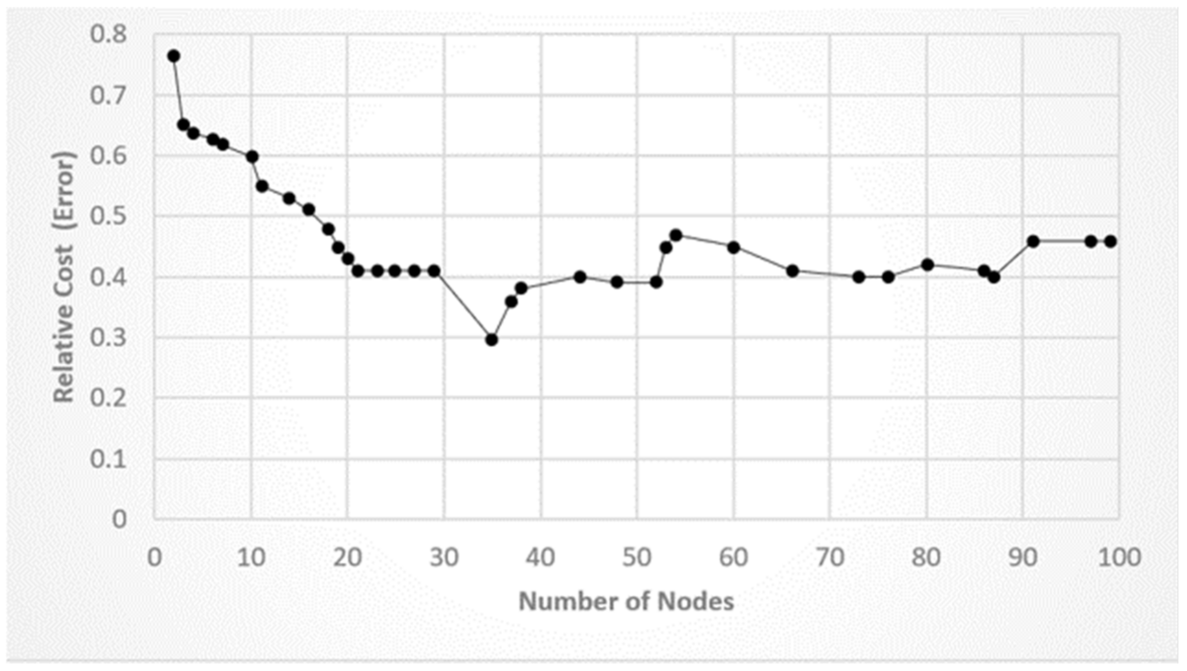
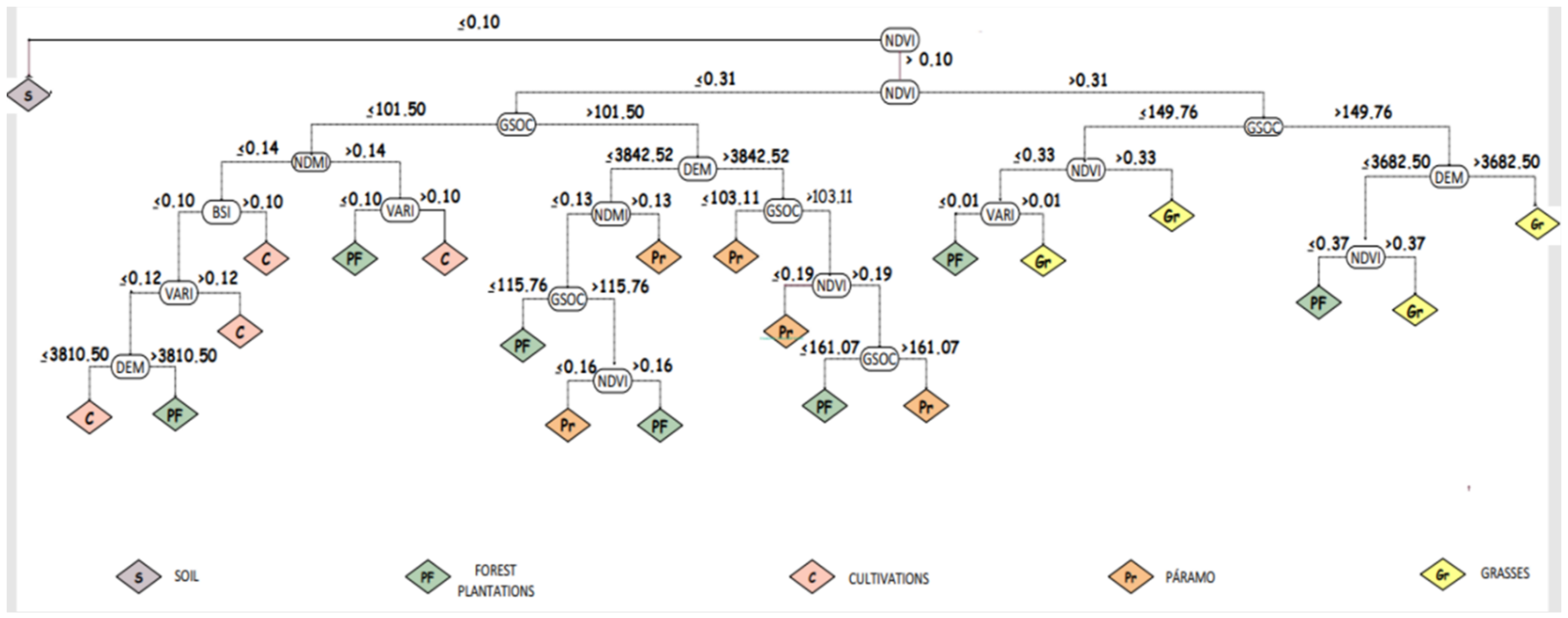
3.4. Optimal Model with Higher Accuracy CDT
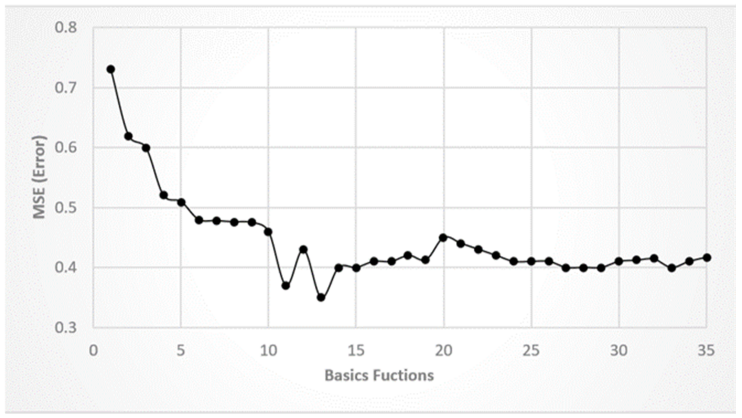
3.5. Optimal Model with Higher Accuracy MARS
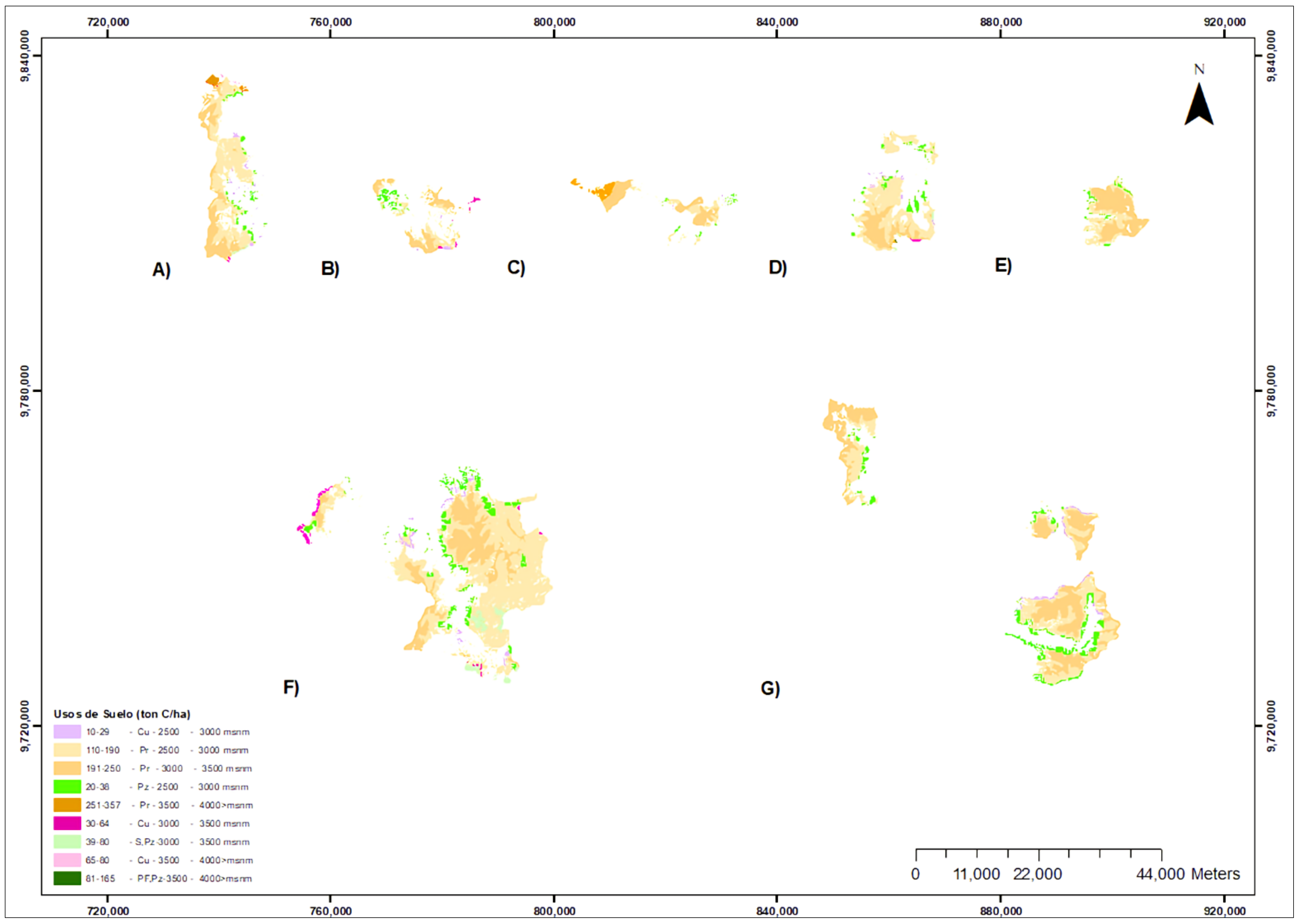
3.6. Distribution of the Categories Researched in the Study Area
3.7. Systematic Land Use Change
4. Conclusions
Author Contributions
Funding
Institutional Review Board Statement
Informed Consent Statement
Data Availability Statement
Acknowledgments
Conflicts of Interest
References
- Castaño, C. Páramos and High Andean Ecosystems of Colombia in Condition of Access Point and Global Climate Tensor; IDEAM: Bogotá, Colombia, 2002. [Google Scholar]
- Crespo, P.; Celleri, R.; Buytaert, W.; Feyen, J.; Iñiguez, V.; Borja, P.; De Bièvre, B. Land use change impacts on the hydrology of wet Andean páramo ecocystems. Status Perspect. Hydrol. Small Basins 2009, 336, 71–76. [Google Scholar] [CrossRef]
- Buytaert, W.; Célleri, R.; De Bievre, B.; Cisneros, F.; Wyseure, G.; Deckers, J.; Hofstede, R. Human impact on the hydrology of the Andean paramos. Earth-Sci. Rev. 2006, 79, 53–72. [Google Scholar] [CrossRef]
- Tonneijck, F.H.; Jansen, B.; Nierop, K.G.J.; Verstraten, J.M.; Sevink, J.; De Lange, L. Towards understanding of carbon stocks and stabilization in volcanic ash soils in natural Andean ecosystems of northern Ecuador. Eur. J. Soil Sci. 2010, 61, 392–405. [Google Scholar] [CrossRef]
- Farley, K.A.; Bremer, L.L.; Harden, C.P.; Hartsig, J. Changes in carbon storage under alternative land uses in biodiverse Andean grasslands: Implications for payment for ecosystem services. Conservation 2012, 6, 21–27. [Google Scholar] [CrossRef]
- Tonneijck, F.H.; Bouten, W.; VanLoon, E.E.; Velthuis, M.; Sevink, J.; Verstraten, J.M. The effect of the change in soil volume on the distribution of organic matter in a volcanic ash soil. Eur. J. Soil Sci. 2016, 67, 226–236. [Google Scholar] [CrossRef]
- Hofstede, R.; Calles, J.; López, V.; Polanco, R.; Torres, F.; Ulloa, J.; Vásquez y Marcos, A.C. Los Páramos Andinos ¿Qué Sabemos? Estado de Conocimiento Sobre el Impacto del Cambio Climático en el Ecosistema Paramo. 2014. Available online: https://portals.iucn.org/library/node/44760 (accessed on 12 February 2021).
- Tian, Q.; He, H.; Cheng, W.; Bai, Z.; Wang, Y.; Zhang, X. Factors controlling soil organic carbon stability along a temperate forest altitudinal gradient. Sci. Rep. 2016, 6, 18783. [Google Scholar] [CrossRef] [Green Version]
- Willis, K.J.; Jeffers, E.S.; Tovar, C. What makes a terrestrial ecosystem resilient? Science 2018, 359, 988–989. [Google Scholar] [CrossRef] [PubMed]
- Chabbi, A.; Rumpel, C. Organic matter dynamics in agro-ecosystems–the knowledge gaps. Eur. J. Soil Sci. 2009, 60, 153–157. [Google Scholar] [CrossRef]
- Luo, Z.; Wang, E.; Sun, O.J. The change of soil carbon and its responses to agricultural practices in Australian agroecosystems: A review and synthesis. Geoderma 2010, 155, 211–223. [Google Scholar] [CrossRef]
- Lal, R.; Pimentel, D.; Van Oost, K.; Six, J.; Govers, G.; Quine, T. Soil erosion: A carbon sink or source? Science 2008, 319, 1040–1042. [Google Scholar] [CrossRef]
- Cholo, T.; Fleskens, L.; Sietz, D.; Peerlings, J. Is land fragmentation facilitating or obstructing adoption of climate adaptation measures in Ethiopia? Sustainability 2018, 10, 2120. [Google Scholar] [CrossRef] [Green Version]
- Ritzema, H.; Kirkpatrick, H.; Stibinger, J.; Heinhuis, H.; Belting, H.; Schrijver, R.; Diemont, H. Water management supporting the delivery of ecosystem services for grassland, heath and moorland. Sustainability 2016, 8, 440. [Google Scholar] [CrossRef] [Green Version]
- Roy, A.; Inamdar, A.B. Multi-temporal Land Use Land Cover (LULC) change analysis of a dry semi-arid river basin in western India following a robust multi-sensor satellite image calibration strategy. Heliyon 2019, 5, e01478. [Google Scholar] [CrossRef] [Green Version]
- Martín, B.; García, M.; Palomo, I.; Montes, C. The conservation against development paradigm in protected areas: Valuation of ecosystem services in the Doñana social–ecological system (southwestern Spain). Ecol. Econ. 2011, 70, 1481–1491. [Google Scholar] [CrossRef]
- Naghavi, H.; Fallah, A.; Shataee, S.; Latifi, H.; Soosani, J.; Ramezani, H.; Conrad, C. Canopy cover estimation across semi-Mediterranean woodlands: Application of high-resolution earth observation data. J. Appl. Remote Sens. 2014, 8, 083524. [Google Scholar] [CrossRef]
- Yu, X.; Hyypp, J.; Vastaranta, M.; Holopainen, M.; Viitala, R. Predicting individual tree attributes from airborne laser point clouds based on the random forests technique. ISPRS J. Photogramm. Remote Sens. 2011, 66, 28–37. [Google Scholar] [CrossRef]
- Steingberg, D.; Colla, P. CART. Classification and Regression Trees; Salford Systems: San Diego, CA, USA, 2016. [Google Scholar]
- Prasad, P.R.C.; Nagabhatla, N.; Reddy, C.S.; Gupta, S.; Rajan, K.S.; Raza, S.H.; Dutt, C.B.S. Assessing forest canopy closure in a geospatial medium to address management concerns for tropical islands-Southeast Asia. Environ. Monit. Assess. 2010, 160, 541–553. [Google Scholar] [CrossRef]
- Suresh, S.; Lal, S. A metaheuristic framework based automated Spatial-Spectral graph for land cover classification from multispectral and hyperspectral satellite images. Infrared Phys. Technol. 2020, 105, 103–172. [Google Scholar] [CrossRef]
- Bi, X.; Chang, B.; Hou, F.; Yang, Z.; Fu, Q.; Li, B. Assessment of spatio-temporal variation and driving mechanism of ecological environment quality in the Arid regions of central asia, Xinjiang. Int. J. Environ. Res. Public Health 2021, 18, 7111. [Google Scholar] [CrossRef]
- Guo, L.; Sun, X.; Fu, P.; Shi, T.; Dang, L.; Chen, Y.; Linderman, M.; Zhang, G.; Zhang, Y.; Jiang, Q.; et al. Mapping soil organic carbon stock by hyperspectral and time-series multispectral remote sensing images in low-relief agricultural areas. Geoderma 2021, 398, 115118. [Google Scholar] [CrossRef]
- Biudes, M.S.; Vourlitis, G.L.; Velasque, M.C.S.; Machado, N.G.; Danelichen, V.H.D.M.; Pavão, V.M.; Arruda, P.H.Z.; Nogueira, J.D.S. Gross primary productivity of Brazilian Savanna (Cerrado) estimated by different remote sensing-based models. Agric. For. Meteorol. 2021, 307, 108456. [Google Scholar] [CrossRef]
- Ienco, D.; Interdonato, R.; Gaetano, R.; Ho Tong Minh, D. Combining Sentinel-1 and Sentinel-2 Satellite Image Time Series for land cover mapping via a multi-source deep learning architecture. ISPRS J. Photogramm. Remote. Sens. 2020, 158, 11–12. [Google Scholar] [CrossRef]
- Tong, X.Y.; Xia, G.S.; Lu, Q.; Shen, H.; Li, S.; You, S.; Zhang, L. Land-cover classification with high-resolution remote sensing images using transferable deep models. Remote Sens. Environ. 2020, 237, 111–122. [Google Scholar] [CrossRef] [Green Version]
- Tajik, S.; Ayoubi, S.; Zeraatpisheh, M. Digital mapping of soil organic carbon using ensemble learning model in Mollisols of Hyrcanian forests, northern Iran. Geoderma Reg. 2020, 20, e00256. [Google Scholar] [CrossRef]
- Marais Sicre, C.; Fieuzal, R.; Baup, F. Contribution of multispectral (optical and radar) satellite images to the classification of agricultural surfaces. Int. J. Appl. Earth Obs. Geoinf. 2020, 84, 101–172. [Google Scholar] [CrossRef]
- Mahmoudzadeh, H.; Matinfar, H.R.; Taghizadeh-Mehrjardi, R.; Kerry, R. Spatial prediction of soil organic carbon using machine learning techniques in western Iran. Geoderma Reg. 2020, 12, 1095. [Google Scholar] [CrossRef]
- Castaldi, F.; Palombo, A.; Santini, F.; Pascucci, S.; Pignatti, S. Evaluation of the potential of the current and forthcoming multispectral and hyperspectral imagers to estimate soil texture and organic carbon. Remote Sens. Environ. 2016, 179, 54–65. [Google Scholar] [CrossRef]
- Guirado, E.; Tabik, S.; Alcaraz-Segura, D.; Cabello, J.; Herrera, F. Deep-Learning Convolutional Neural Networks for scattered shrub detection with Google Earth Imagery. Remote Sens. 2017, 9, 1706. [Google Scholar]
- Cheng, W.; Zhang, X.; Wang, K.; Dai, X. Integrating classification and regression tree (CART) with GIS for assessment of heavy metals pollution. Environ. Monit. Assess. 2009, 158, 419–431. [Google Scholar] [CrossRef]
- Lees, B.G.; Ritman, K. Decision-tree and rule-induction approach to integration of remotely sensed and GIS data in mapping vegetation in disturbed or hilly environments. Environ. Manag. 1991, 15, 823–831. [Google Scholar] [CrossRef]
- Lu, D.; Mausel, P.; Brondizio, E.; Moran, E. Change detection techniques. Int. J. Remote Sens. 2004, 25, 2365–2407. [Google Scholar] [CrossRef]
- Emamgolizadeh, S.; Bateni, S.M.; Shahsavani, D.; Ashrafi, T.; Ghorbani, H. Estimation of soil cation exchange capacity using Genetic Expression Programming (GEP) and Multivariate Adaptive Regression Splines. J. Hydrol. 2015, 529, 1590–1600. [Google Scholar] [CrossRef]
- Kuter, S.; Akyurek, Z.; Weber, G. Remote Sensing of Environment Retrieval of fractional snow covered area from MODIS data by multivariate adaptive regression splines. Remote Sens. Environ. 2018, 205, 236–252. [Google Scholar] [CrossRef]
- MAE. Ministerio del Ambiente del Ecuador, Sistema de Clasificación de los Ecosistemas del Ecuador Continental; Subsecretaría de Patrimonio Natural: Quito, Ecuador, 2012.
- Padró, J.; Muñoz, F.; Ávila, L.; Pesquer, L.; Pons, X. Radiometric Correction of Landsat-8 and Sentinel-2A Scenes Using Drone Imagery in Synergy with Field Spectroradiometry. Remote Sens. 2018, 10, 1687. [Google Scholar] [CrossRef] [Green Version]
- IGM, Geoportal. 2016. Available online: http://www.igm.gob.ec/index.php/en/servicios (accessed on 16 February 2009).
- QGIS Development Team QGIS Geographic Information System. Open Source Geospatial Foundation Project. 2020. Available online: http://qgis.osgeo.org (accessed on 14 September 2020).
- Comité de la Subcuenca Chambo. Aportes a la Planificación Para la Gestión Integral de Los Recursos Hídricos; CESA: Riobamba, Ecuador, 2015. [Google Scholar]
- FAO. Food and Agriculture Organization of the United Nations; Global Soil Organic Carbon: Roma, Italy, 2017. [Google Scholar]
- Ayala, J.; Márquez, C.; García, V.; Recalde-Moreno, C.G.; Rodríguez-Llerena, M.V.; Damián-Carrión, D.A. Land cover classification in an Ecuadorian mountain geosystem using a random forest classifier, spectral vegetation indices, and ancillary geographic data. Geoscience 2017, 7, 34. [Google Scholar] [CrossRef] [Green Version]
- Conoscenti, C.; Ciaccio, M.; Caraballo-arias, N.A.; Gómez-gutiérrez, A.; Rotigliano, E.; Agnesi, V. Geomorphology Assessment of susceptibility to earth- flow landslide using logistic regression and multivariate adaptive regression splines: A case of the Belice River basin (western Sicily, Italy). Geomorphology 2015, 242, 49–64. [Google Scholar] [CrossRef]
- Rouse, J.W.; Haas, R.H.; Schell, J.A.; Deering, D.W. Monitoring Vegetation Systems in the Great Plains with ERTS; Freden, S.C., Mercanti, E.P., Becker, M.A., Eds.; Third Earth Resources Technology Satellite-1 Symposium-Volume I: Technical Presentations. NASA SP-351; NASA: Washington, DC, USA, 1974; pp. 309–335.
- Huete, A.R. A soil-adjusted vegetation index (SAVI). Remote Sens. Environ. 1988, 25, 295–309. [Google Scholar] [CrossRef]
- Gitelson, A.A.; Kaufman, Y.J.; Stark, R.; Rundquist, D. New algorithms for remote estimation of the vegetation fraction. Remote Sens. 2002, 80, 76–87. [Google Scholar]
- Jiang, Z.; Huete, A.R.; Didan, K.; Miura, T. Development of a two-band enhanced vegetation index without a blue band. Remote Sens. Environ. 2008, 112, 3833–3845. [Google Scholar] [CrossRef]
- Chen, W.; Liu, L.; Zhang, C.; Li, S.; Chen, X. A new bare-soil index for rapid mapping developing areas using LANDSAT 8 data. Int. Soc. Photohrammetry Remote Sens. 2004, 40, 139. [Google Scholar] [CrossRef] [Green Version]
- Fisher, R.A. Statistical Methods and Scientific Inference; Oxford University Press: Oxford, UK, 1991. [Google Scholar]
- Awiti, A.; Walsh, M.; Shepherd, K.; Kinyamario, J. Soil Condition classification using infrared spectroscopy: A proposition for assessment of soil condition along a tropical forest-cropland chronosequence. Geoderma 2008, 143, 73–84. [Google Scholar] [CrossRef]
- Michaelsen, J.; Schimel, D.S.; Friedl, M.A.; Davis, F.W.; Dubayah, R.C. Regression Tree Analysis of satellite and terrain data to guide vegetation sampling and surveys. J. Veg. Sci. 1994, 5, 673–686. [Google Scholar] [CrossRef]
- Asrar, G.; Fuchs, M.; Kanemasu, E.T.; Hatfield, J.L.; Yoshida, M. Estimates of leaf area index from spectral reflectance of wheat under different cultural practices and solar angle. Remote Sens. Environ. 1984, 17, 300–306. [Google Scholar] [CrossRef]
- Pontius, R.G.; Shusas, E.; McEachern, M. Detecting important categorical land changes while accounting for persistence. Agric. Ecosyst. Environ. 2004, 101, 251–268. [Google Scholar] [CrossRef]
- Sherman, G. The PyQGIS Programmer′s Guide; Locate Press: London, UK, 2014. [Google Scholar]
- Fernández, G.F.; Obermeier, W.A.; Gerique, A.; López, M.F.; Lehnert, L.W. Land cover change in the Andes of Southern Ecuador—Patterns and drivers. Remote Sens. 2015, 7, 2509–2542. [Google Scholar] [CrossRef] [Green Version]
- Salford Predictive Modeler Machine Learning and Predictive Analytics Software. 2018. Available online: https://www.salford-systems.com (accessed on 12 February 2019).
- Spearman, C.E. “General intelligence”, objectively determined and measured. Am. J. Psychol. 1904, 15, 201–293. [Google Scholar] [CrossRef]
- Kweku, M.; Osei, B. Post-pruning in regression tree induction: An integrated approach. Expert Syst. Appl. 2008, 34, 1481–1490. [Google Scholar] [CrossRef]
- Breiman, L.; Friedman, J.; Olshen, R.; Stone, C. Classification and Regression Trees; Mathematics & Statistics: Boca Raton, FL, USA, 1984. [Google Scholar]
- Heredia, S.E.; Bruno, C.; Balzarini, M. Identification of relationships between yields and environmental variables via classification and regression trees (CART). Interciencia 2010, 35, 876–882. [Google Scholar]
- Chen, W.; Xie, X.; Wang, J.; Pradhan, B.; Hong, H.; Bui, D.T.; Duan, Z.; Ma, J. A comparative study of logistic model tree, random forest, and classification and regression tree models for spatial prediction of landslide susceptibility. CATENA 2017, 151, 147–160. [Google Scholar] [CrossRef] [Green Version]
- Friedman, J.H.; Hastie, T.; Tibshirani, R. Additive logistic regression: A statistical view of boosting. Ann. Stat. 2000, 28, 337–407. [Google Scholar] [CrossRef]
- Francis, L. Neural Networks Demystified. In Proceedings of the Casualty Actuarial Society Forum, Winter, Las Vegas, NV, USA, 12–13 March 2001; pp. 253–320. [Google Scholar]
- Lewis, P.A.; Stevens, J.G. Nonlinear Modeling of Time Series Using Multivariate Adaptive Regression Splines (MARS). J. Am. Stat. Assoc. 1991, 86, 416–450. [Google Scholar] [CrossRef]
- Hansen, P.M.; Schjoerring, J.K. Reflectance measurement of canopy biomass and nitrogen status in wheat crops using normalized difference vegetation indices and partial least squares regression. Remote Sens. Environ. 2003, 86, 542–553. [Google Scholar] [CrossRef]
- Bhunia, G.S.; Shit, P.K.; Pourghasemi, H.R. Soil organic carbon mapping using remote sensing techniques and multivariate regression model. Geocarto Int. 2017, 5, 2–25. [Google Scholar] [CrossRef]
- García, V.; Márquez, C.; Isenhart, T.; Rodríguez, M.; Crespo, S.; Cifuentes, A. Evaluating the conservation state of the paramo ecosystem: An object-based image analysis and CART algorithm approach for central Ecuador. Heliyon 2019, 5, e02701. [Google Scholar] [CrossRef] [PubMed] [Green Version]
- Fisher, R.A. On the Probable Error of a Coefficient of Correlation Deduced from a Small Sample. Metron 1921, 2, 3–32. [Google Scholar]
- Fleishman, A. A method for simulating non-normal distributions. Psychometrika 1978, 43, 521–531. [Google Scholar] [CrossRef]
- Dempsted, A.P.; Laird, N.M.; Rubin, D.B. Maximun likelihood from incomplete data via the EM algorithm. J. Am. Stat. Assoc. 1977, 81, 41–60. [Google Scholar]
- Kuhn, N.; Hoffmann, T.; Schwanghart, W.; Dotterweich, M. Agricultural soil erosion and global carbon cycle: Controversy over? Earth Surf. Process. Landf. 2009, 34, 1033–1038. [Google Scholar] [CrossRef]
- Peters, M.K.; Hemp, A.; Appelhans, T.; Becker, J.N.; Behler, C.; Classen, A.; Detsch, F.; Ensslin, A.; Ferger, S.W.; Frederiksen, S.B.; et al. Climate–land-use interactions shape tropical mountain biodiversity and ecosystem functions. Nature 2019, 568, 88–92. [Google Scholar] [CrossRef]
- Rubin, D.B.; Schenker, N. Interval estimation from multiply-imputed data: A case study using census agriculture industry codes. J. Off. Stat. 1987, 60, 375–387. [Google Scholar]


| Index | Formula | Characteristics |
|---|---|---|
| NDVI: Normalized difference vegetation index | Minimizes topographic effects and produces a linear measurement scale. Negative values represent areas without vegetation. The higher the index is, the higher the chlorophyll index is [45]. | |
| SAVI: Soil-adjusted vegetation index | Minimizes the effect of the soil in areas with low vegetation density [46]. | |
| VARI: Visible atmospherically resistant index | It highlights vegetation in the visible part of the spectrum, while mitigating differences in lighting and atmospheric effects [47]. | |
| EVI: Improved vegetation index | It corrects some atmospheric conditions, e.g., the background noise of the canopy, and it is more sensitive in areas with dense vegetation [48]. | |
| BSI: Bare soil index | The difference in the number of areas of bare soil, land, and vegetation [49]. | |
| NGRDI: Normalized red green difference index | Reflectance of the green and red area of the electromagnetic spectrum, which come from a true color image [49]. | |
| ARVI: Atmospheric resistant vegetation index | Recommended for areas with a high concentration of some type of aerosol, mist, smoke, or other type of particles suspended in the air [50]. | |
| GCI: Green coverage index | It can specify the health status of the vegetation or warn of the start of temporary seasons [47]. | |
| GNDVI: Green normalized difference vegetation index | It is a measure of the “greenness” of the plant or photosynthetic activity. This index is mainly used in the intermediate and final stages of the crop cycle [45]. | |
| NDMI: Normalized difference moisture index | It describes the level of water stress of the vegetation and between the difference and the sum of the radiation refracted in the near-infrared and SWIR [51]. |
| Measurement | Formula-Defines Each Parameter in the Description | Description |
|---|---|---|
| Producer’s accuracy (PA) | Producer’s accuracy is a reference-based accuracy that is computed by reviewing the predictions produced by a class and by establishing the percentage of correct predictions [52]. | |
| User’s accuracy (UA) | User’s accuracy is a map-based accuracy that is computed by reviewing the reference data for a class and establishing the percentage of correct predictions for these samples [53]. | |
| Overall accuracy (OA) | Indicates the proportion of all reference pixels that are correctly classified [53]. | |
| Kappa index | Concordance between the observed values of the image and the values estimated by the classifier [13]. | |
| Indicators of change Gain Losses Net change | Gain (Gij) = P+j − Pjj Losses (Lij) = Pj+ − Pjj Net Change (Dj) = l Lij − Gij l Total change (DTJ) = Gij + Lij Exchange (Sj) = 2 × MIN (Pj+ − Pjj, P+j − Pjj) | They make it possible to determine for each category gains, losses, net change, and exchanges experienced between two points in time [54]. |
| Systematic transitions in terms of gain and loss | A latent transition is interpreted as existing but apparently inactive and an active transition means that it works or has the capacity to act [54]. |
| NDVI | VARI | BSI | NDMI | |
|---|---|---|---|---|
| NDVI | 1.00 | |||
| VARI | 0.62 | 1.00 | ||
| BSI | −0.75 | −0.84 | 1.00 | |
| NDMI | 0.78 | 0.77 | −0.99 | 1.00 |
| Class | L | V | PF(L) | PF(V) | C(L) | C(V) | Pr(L) | Pr(V) | Gr(L) | Gr(V) | S(L) | S(V) | UA(L) | UA(V) | PA(L) | PA(V) |
|---|---|---|---|---|---|---|---|---|---|---|---|---|---|---|---|---|
| PF | 150 | 47 | 117 | 39 | 7 | 3 | 6 | 2 | 19 | 2 | 1 | 1 | 78 | 70.21 | 73.13 | 73.13 |
| C | 700 | 267 | 8 | 13 | 580 | 213 | 75 | 18 | 29 | 15 | 8 | 8 | 82.86 | 79.78 | 83.09 | 83.09 |
| Pr | 1600 | 540 | 16 | 3 | 55 | 33 | 1400 | 436 | 112 | 43 | 17 | 5 | 87.5 | 83.85 | 87.99 | 87.99 |
| Gr | 1290 | 273 | 19 | 4 | 41 | 15 | 101 | 26 | 1110 | 226 | 19 | 2 | 86.05 | 82.78 | 87.06 | 87.06 |
| S | 175 | 47 | 0 | 0 | 15 | 2 | 9 | 2 | 5 | 5 | 146 | 38 | 83.43 | 80.85 | 76.44 | 76.44 |
| Total | 3915 | 1174 |
| Class | L | V | PF(L) | PF(V) | C(L) | C(V) | Pr(L) | Pr(V) | Gr(L) | Gr(V) | S(L) | S(V) | UA(L) | UA(V) | PA(L) | PA(V) |
|---|---|---|---|---|---|---|---|---|---|---|---|---|---|---|---|---|
| PF | 150 | 47 | 105 | 30 | 10 | 8 | 11 | 6 | 18 | 3 | 6 | 0 | 70.00 | 63.83 | 65.63 | 65.63 |
| C | 700 | 267 | 14 | 10 | 510 | 185 | 106 | 61 | 68 | 9 | 2 | 2 | 72.86 | 69.29 | 70.83 | 70.83 |
| Pr | 1600 | 540 | 21 | 1 | 110 | 73 | 1200 | 380 | 241 | 82 | 28 | 4 | 75.00 | 70.37 | 79.52 | 79.52 |
| Gr | 1290 | 273 | 20 | 6 | 80 | 22 | 167 | 35 | 1007 | 201 | 16 | 9 | 78.06 | 73.63 | 75.09 | 75.09 |
| S | 175 | 47 | 0 | 0 | 10 | 5 | 25 | 4 | 7 | 5 | 133 | 33 | 76.00 | 70.21 | 71.89 | 71.89 |
| Total | 3915 | 1174 |
| Algorithms | OA (L)% | OA (V)% | KAPPA (L)% | KAPPA (V)% |
|---|---|---|---|---|
| CDT | 88.00 | 83.84 | 86.51 | 83.49 |
| MARS | 81.83 | 75.46 | 79.86 | 74.92 |
| Type | Conditionals | Observation |
|---|---|---|
| C | NDVI ≤ 0.31, GSOC ≤ 101.50, NDMI > 0.14, VARI > 0.10 NDVI ≤ 0.31, GSOC ≤ 101.50, NDMI ≤ 0.14, BSI > 0.10 NDVI ≤ 0.31, GSOC ≤ 101.50, NDMI ≤ 0.14, BSI ≤ 0.10, VARI > 0.12 NDVI ≤ 0.31, GSOC ≤ 101.50, NDMI ≤ 0.14, BSI ≤ 0.10, VARI ≤ 0.12, DEM ≤ 3810.50 | NDMI is the most important variable in determining crops indicating that crop leaf sensitivity and canopy water stress are directly related to crop development. |
| Pr | NDVI ≤ 0.31, GSOC > 101.50, DEM ≤ 3842.52, NDMI > 0.13 NDVI ≤ 0.31, GSOC > 101.50, DEM > 3842.52, GSOC ≤ 103.11 NDVI ≤ 0.31, GSOC > 101.50, DEM > 3842.52, GSOC > 103.11, NDVI ≤ 0.19 NDVI ≤ 0.31, GSOC > 101.50, DEM ≤ 3842.52, NDMI ≤ 0.13, GSOC > 115.76, NDVI ≤ 0.16 NDVI ≤ 0.31, GSOC > 101.50, DEM > 3842.52, GSOC > 103.11, NDVI > 0.19, GSOC > 161.07 | Altitude is one of the variables that significantly determined the distribution of the ecosystem (Pr). The ecosystem can develop above 3842.52 m.a.s.l. |
| Gr | NDVI > 0.31, GSOC ≤ 149.76, NDVI > 0.33 NDVI > 0.31, GSOC > 149.76, DEM > 3682.50 NDVI > 0.31, GSOC ≤ 149.76, NDVI ≤ 0.33, VARI > 0.01 NDVI > 0.31, GSOC > 149.76, DEM ≤ 3682.50, NDVI > 0.37 | The tree determined Gr coverage in two very interesting branches. In one of the branches, the DEM variable is determinant while in the other branch it is not, which leads us to think that the predictive model could be defining one category of natural pasture and another of cultivated pasture. That is, it moves towards natural areas without any control. |
| PF | NDVI > 0.31, GSOC ≤ 149.76, NDVI ≤ 0.33, VARI ≤ 0.01 NDVI ≤ 0.31, GSOC ≤ 101.50, NDMI > 0.14, VARI ≤ 0.10 NDVI > 0.31, GSOC > 149.76, DEM ≤ 3682.50, NDVI ≤ 0.37 NDVI ≤ 0.31, GSOC > 101.50, DEM ≤ 3842.52, NDMI ≤ 0.13, GSOC ≤ 115.76 NDVI ≤ 0.31, GSOC > 101.50, DEM ≤ 3842.52 NDMI ≤ 0.13, GSOC > 115.76 > 0.16 NDVI ≤ 0.31, GSOC ≤ 101.50, NDMI ≤ 0.14, BSI ≤ 0.10, VARI ≤ 0.12, DEM > 3810.50 NDVI ≤ 0.31, GSOC > 101.50, DEM > 3842.52, GSOC > 103.11 > 0.19, GSOC ≤ 161.07 | Forest plantation coverage (FP) has the lowest prediction percentage. It is important to mention that it has the lowest proportioned coverage in the area, so field monitoring could improve its performance. |
| S | NDVI ≤ 0.10 | The NDVI variable was sufficient to determine the ground cover. |
| Coverage | Gains % | Losses% | Exchange% | Net Change% |
|---|---|---|---|---|
| Pr | 7.65 | 16.65 | 12.76 | 7.93 |
| C | 2.15 | 1.52 | 3.04 | 0.63 |
| Gr | 7.84 | 0.32 | 0.64 | 7.52 |
| PF | 1.53 | 0.98 | 1.96 | 0.55 |
| S | 5.11 | 0.18 | 0.36 | 4.93 |
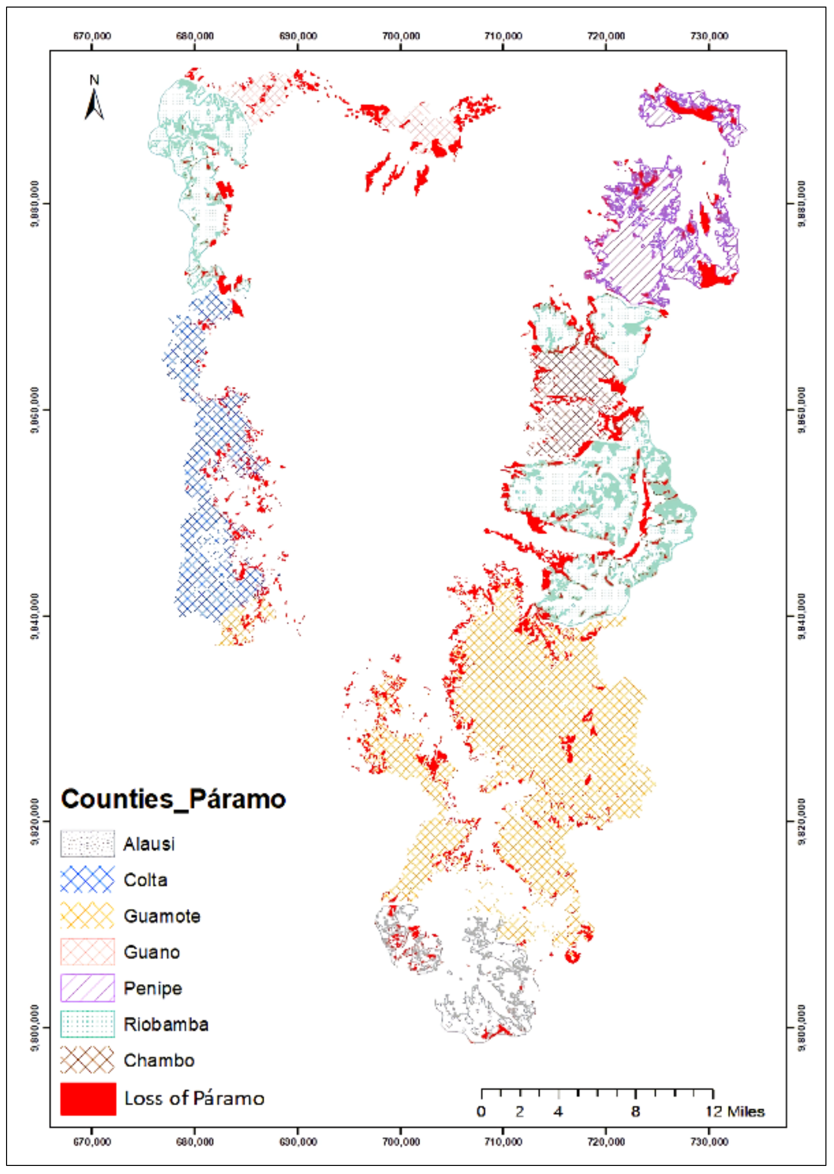
| Loss of PÁRAMO from the Coverage Studied 2012–2020 (Ha) | Loss of PÁRAMO from the Coverage Studied 2012–2020 (%) | ||||||||||||
|---|---|---|---|---|---|---|---|---|---|---|---|---|---|
| County | UTM Coordinates—Zone 17 Southern Hemisphere | Pr-MAE (2012) | C | Gr | PF | S | Total | C | Gr | PF | S | Total | |
| X | Y | ||||||||||||
| ALAUSÍ | 766,363.14 | 9,750,636.59 | 5176.00 | 181.12 | 307.12 | 241.14 | 55.99 | 785.38 | 0.14 | 0.24 | 0.19 | 0.04 | 0.61 |
| CHAMBO | 777,562.97 | 9,805,829.89 | 8220.56 | 172.96 | 418.00 | 107.20 | 645.68 | 1343.84 | 0.13 | 0.33 | 0.08 | 0.50 | 1.05 |
| COLTA | 742,465.20 | 9,799,454.32 | 14,454.90 | 254.01 | 1093.07 | 47.87 | 5.93 | 1400.88 | 0.20 | 0.85 | 0.04 | 0.01 | 1.09 |
| GUAMOTE | 770,637.10 | 9,772,754.27 | 48,481.67 | 593.87 | 2488.48 | 687.05 | 1590.00 | 5359.40 | 0.46 | 1.94 | 0.54 | 1.24 | 4.18 |
| GUANO | 755,657.56 | 9,833,453.54 | 5291.30 | 236.08 | 824.65 | 175.89 | 975.87 | 2212.49 | 0.18 | 0.64 | 0.14 | 0.76 | 1.73 |
| PENIPE | 786,059.27 | 9,823,700.11 | 13,667.04 | 182.86 | 940.97 | 364.46 | 607.79 | 2096.09 | 0.14 | 0.73 | 0.28 | 0.47 | 1.64 |
| RIOBAMBA | 769,782.92 | 9,806,343.65 | 32,879.01 | 1148.02 | 3988.42 | 333.53 | 2678.06 | 8148.02 | 0.90 | 3.11 | 0.26 | 2.09 | 6.36 |
| 128,170.48 | 21,346.10 | 16.65 | |||||||||||
| Coverage | Footprint Size | Strength of the Transition | Interpretation |
|---|---|---|---|
| Pr a C | −0.16 | −0.37 | Cultivation gains, cultivation does not replace páramo. |
| Pr a Gr | 0.11 | 0.02 | Grassland gains, grassland replaces páramo. |
| Pr a PF | −0.81 | −0.95 | Plantation forest gains, plantation forest does not replace páramo. |
| Pr a S | −3.11 | −0.93 | Soil gains, Soil does not replace páramo. |
| C a Pr | −0.03 | −0.33 | Páramo gains, páramo does not replace crop. |
| C a Gr | 0.33 | 0.89 | Grassland gains, grassland replaces crop. |
| C a PF | −0.35 | −7.00 | Plantation forestry gains, forest plantation does not replace cultivation. |
| C a S | 0.11 | 0.58 | Soil gains, soil replaces crop. |
| Gr a Pr | −0.17 | −0.85 | Páramo gains, páramo does not replace grassland. |
| Gr a C | −0.01 | −0.20 | Crop gains, crop does not replace grassland. |
| Gr a PF | −0.01 | −0.09 | Plantation forest gains, forest plantation does not replace grassland. |
| Gr a S | −2.58 | −6.14 | Soil gains, soil does not replaces grassland. |
| PF a C | 0.03 | 4.00 | Crop gains, crop replaces forest plantation. |
| PFa Gr | 0.04 | 0.94 | Grassland gains, grassland replace forest plantation. |
| PF a S | 0.15 | 5.25 | Soil gains, soil replaces forest plantation. |
| S a Pr | −0.23 | −3.29 | Páramo gains, páramo does not replaces soil. |
| S a C | −0.13 | −6.50 | Crop gains, crop does not replaces soil. |
| S a Gr | −0.29 | −0.97 | Grassland gains, grassland does not replace soil. |
| S a PF | −0.46 | −11.50 | Plantation forestry gains, plantation forestry does not replaces soil. |
| Coverage | Footprint Size | Strength of the Transition | Interpretation |
|---|---|---|---|
| Pr a C | −0.70 | −0.72 | Páramo loses, crop does not replace páramo. |
| Pr a Gr | 2.87 | 0.75 | Páramo loses, pastizal replaces páramo. |
| Pr a PF | −0.61 | −0.94 | Páramo loses, forest plantation does not replace páramo. |
| Pr a S | −1.56 | −0.86 | Páramo loses, soil does not replace páramo. |
| C a Pr | −1.05 | −0.95 | Crop loses, páramo does not replace crop. |
| C a Gr | 0.49 | 2.33 | Crop loses, grassland replaces crop. |
| C a PF | −0.36 | −9.00 | Crop loses, plantation forestry does not replace crop. |
| C a S | 0.20 | 2.00 | Crop loses, soil replaces crop. |
| Gr a Pr | −2.67 | −0.99 | Grassland loses, páramo does not replace grassland. |
| Gr a C | −0.09 | −0.69 | Grassland loses, crop does not replace grassland. |
| Gr a PF | −0.01 | −0.11 | Grassland loses, plantation forestry does not replace grassland. |
| Gr a S | −2.75 | −11.00 | Grassland loses, soil does not replace grassland. |
| PF a Pr | −0.42 | −0.98 | Forest plantation loses, páramo does not replace forest plantation. |
| PF a C | 0.03 | 1.50 | Forest plantation loses, crop replaces forest plantation. |
| PFa Gr | −0.07 | −0.88 | Forest plantation loses, grassland does not replace forest plantation. |
| PF a S | 0.46 | 11.50 | Forest plantation loses, grassland replaces forest plantation. |
| S a Pr | −0.45 | −0.60 | Soil loses, páramo does not replace soil. |
| S a C | −0.11 | −2.75 | Soil loses, crop does not replaces soil. |
| S a Gr | −0.14 | −0.93 | Soil loses, grassland does not replace soil. |
| S a PF | −0.48 | −15.00 | Soil loses, plantation forestry does not replace soil. |
Publisher’s Note: MDPI stays neutral with regard to jurisdictional claims in published maps and institutional affiliations. |
© 2021 by the authors. Licensee MDPI, Basel, Switzerland. This article is an open access article distributed under the terms and conditions of the Creative Commons Attribution (CC BY) license (https://creativecommons.org/licenses/by/4.0/).
Share and Cite
Pazmiño, Y.; de Felipe, J.J.; Vallbé, M.; Cargua, F.; Quevedo, L. Identification of a Set of Variables for the Classification of Páramo Soils Using a Nonparametric Model, Remote Sensing, and Organic Carbon. Sustainability 2021, 13, 9462. https://0-doi-org.brum.beds.ac.uk/10.3390/su13169462
Pazmiño Y, de Felipe JJ, Vallbé M, Cargua F, Quevedo L. Identification of a Set of Variables for the Classification of Páramo Soils Using a Nonparametric Model, Remote Sensing, and Organic Carbon. Sustainability. 2021; 13(16):9462. https://0-doi-org.brum.beds.ac.uk/10.3390/su13169462
Chicago/Turabian StylePazmiño, Yadira, José Juan de Felipe, Marc Vallbé, Franklin Cargua, and Luis Quevedo. 2021. "Identification of a Set of Variables for the Classification of Páramo Soils Using a Nonparametric Model, Remote Sensing, and Organic Carbon" Sustainability 13, no. 16: 9462. https://0-doi-org.brum.beds.ac.uk/10.3390/su13169462