Developing a Traffic Model to Estimate Vehicle Emissions: An Application in Seoul, Korea

Abstract

In this study, a traffic demand model was created based on a simulation network, and another model was built to calculate exhaust-gas emissions generated by vehicles based on the emission function. Subsequently, emissions for three scenarios were analyzed based on the traffic restriction policy according to the vehicle grading system implemented in Seoul. According to the results of the analysis, emission reduction under the vehicle restriction policy was the highest among passenger cars in the low-speed range, while the emissions of cargo trucks in the high-speed range were found to be high. The emissions showed a high ratio of carbon monoxide and nitrogen oxides, and high emissions were generated from liquefied petroleum gas and diesel vehicles. Furthermore, the effects of vehicle restriction policy were confirmed to reduce emissions from diesel and other vehicle types. Using the established model, we were able to confirm that the vehicle restriction policy contributed to the improvement of air quality. Furthermore, the diesel vehicle restriction policy also had an impact on reducing the emissions of vehicle types other than those using diesel.

1. Introduction

The annual global death toll from air pollution has continued to increase from 1.3 million in 2011 to 4.2 million in 2020 (World Health Organization) [1]. Recognizing the severity of air pollutants, major cities worldwide are seeking various measures to reduce emissions and implementing relevant policies accordingly [2,3]. The transportation sector accounts for 30% of urban air pollution in cities; this segment is considered the most important focus for maintaining clean air quality and healthy urban environments [4]. In most large cities that rely on fossil-fuel-based traffic modes, several policies have been considered as potential solutions to this issue. Representative transportation policies include the vehicle grade system and emission regulation policies, which are enforced worldwide, and the standards for each country are applied as a domestic standard. The most representative vehicle emission standard is Euro 6. In Europe, Euro 6 was applied as the emission standard for light-duty vehicles from 2014 to 2020 and for heavy-duty vehicles from 2013 to 2020. From March 2020, it was regulated by applying the emissions standard corresponding to Euro 7. In addition, several Chinese cities with severe air quality are working to improve their air quality by implementing the China 6a∙6b [5]. However, it is not always easy to determine how effective these policies might be, because air quality in cities is a result of complex processes contributed by multiple sectors. Assessing how much a specific subdivision has affected the overall air quality is difficult.

Continuous research is conducted to develop a method for calculating the exhaust emissions of vehicles on the road. Many variables must be considered in this context, which requires a vast amount of traffic data and vehicle characteristics data [6]. Traffic volume may vary depending on the actual road condition, traffic policy, and driver’s behavior; in turn, these conditions will impact a vehicle’s travel speed. In addition, because exhaust emissions also vary according to the properties of different vehicles, a significant effort is required to appropriately calculate the emissions of different vehicles being driven on the road [7].

Accordingly, this study aimed to develop a model for calculating the exhaust emissions of vehicles in Seoul and the emissions of air pollutants generated by the traffic on road networks. In addition, based on the Seoul Municipal Government’s scenario of restricting access to specific areas under the vehicle grade system, we intended to determine the reduction in vehicle emissions owing to relevant policies, using a simulation network.

The purpose of this study was to create a traffic demand model based on a simulation network and to develop a model for calculating the exhaust emissions from vehicles by linking the traffic demand model to specific emission functions. Based on the developed model, we aimed to review the traffic restriction policy according to the vehicle grade system in urban areas of Seoul as a basic scenario and to analyze changes in the emissions for three scenarios.

The Sioux Falls network was adopted as the network to be simulated for the analysis in this study. We aimed to confirm the simulation results according to the particular scenario based on the emission calculation traffic model we created. The three adopted scenarios are shown in

Table 1. Research scenarios based on the vehicle grading system.

Division	Contents of Scenario
Scenario 0	When the vehicle restriction is not implemented
Scenario 1	When grade 5 diesel vehicles are restricted (current)
Scenario 2	When grades 4 & 5 diesel vehicles are restricted

.

2. Literature Review

2.1. Studies on the Calculation of Vehicle Emissions

As the severity of greenhouse gases and air pollutants resulting from vehicle use in the city continues to grow, ongoing research has focused on calculating the level of emissions generated in this context. These quantities have been calculated in various ways, some of which are presented below.

Studies on emission substances and their levels, based on vehicle speed and platooning, were conducted in the following. In the study of Lv and Zhang (2012), vehicle platooning caused by the acceleration, deceleration, and stopping of vehicles due to signal coordination was expected to affect emissions [8]. Emissions were found to increase as the number of stops of the vehicle was greater than that of the vehicle’s platoon ratio. Panis et al., (2006) considered the effect of changes in the vehicle’s travel speed on emissions via active speed management. They found that although the average speed of the vehicle decreased by speed management, the emissions did not appear to decrease directly. The effect on emissions was considered to have an effect not only on the average speed but also on a complex part [9]. These studies analyzed the total emissions generated depending on the vehicle’s acceleration/deceleration, as well as the travel speed, and found that emission levels were the highest when a vehicle stopped and lowest when the average speed was 65 km/h [10]. Rodríguez et al., (2016) analyzed the vehicle specific power to calculate mobile pollution sources based on speed and acceleration. The analysis targets were low-speed driving due to traffic jams, which affect emissions. In this context, it is expected that emissions can be improved through hybrid vehicles [11]. In the study of Osorio and Nanduri (2015), emissions were calculated through a high-resolution micro-traffic model. The model used for analysis is superior to the model using only analysis information or simulation information. In the model, nitrogen oxides (NOx), volatile organic compounds (VOC), and PM concentrations were affected by individual vehicle properties or complex local traffic dynamics [12]. Cho et al., (2012) calculated emission pollutant coefficients according to vehicle speed and calculated emissions by vehicle type. Experiments were performed to calculate the emissions as they vary according to the speed of the vehicle. [13]. Zhu and Zhang (2017) calculated the exhaust emissions from vehicles considering acceleration/deceleration caused by adhering to traffic signals [14]. Considering that the emissions were affected by speed and acceleration, Kun and Lei (2007) analyzed and calculated a vehicle’s exhaust emissions using the VISSIM and emission amount models [15]. However, this study was limited because not all vehicle models and fuels could be included, and vehicles’ model year was not considered.

Emission results varied based on the individual characteristics of a vehicle and its speed. Vehicle characteristics such as vehicle type and size, the specific fuel used, and the model year all affected emissions, and the amount of the discharged substance varied according to each characteristic. However, considering the emissions for all vehicles within a broad spatial range and over a long time is limited by currently available technology. Several studies have, nonetheless, aimed to calculate emissions based on the consideration of vehicle characteristics in specific cases, despite not including all of the vehicles involved. Examples include studies conducted by Panis et al., (2006), Huang et al., (2017), Borge et al., (2016), Outapa et al., (2018), and Song and Hao (2021) [9,16,17,18,19]. Panis et al., (2006) distinguished between the fuel and vehicle type and conducted a relevant analysis, based on varying carbon dioxide emissions as a result of vehicle acceleration and speed [9]. Huang et al., (2017) calculated emissions based on different substances according to vehicle characteristics in a tunnel in Shanghai (China) and considered the different substance emissions from vehicles [16]. Outapa et al., (2018) compared European emission models with international vehicle emission models and then examined emission factors of actually driven trucks. For a more-developed model, the emission source and characteristics of the vehicle should be considered [18]. Song and Hao (2021) considered the emissions for each substance by employing a commonly used vehicle emission calculation formula. In addition, they created nine scenarios, based on the vehicle pollutant emission reduction policy implemented in China, to confirm the degree of emissions reduction according to the policy [19].

Existing studies commonly aimed to consider as many characteristics as possible. However, these studies included limitations due to data restrictions and differences from real-world situations. In addition, based on differences in the spatial range under consideration for each model, the amount and type of emissions generated varied. Furthermore, while a larger set of properties could be considered in the model for a small area, the model was limited in terms of doing the same for a wide range of areas. In the case of the emission function that is applied in Korea, the limitations were that it does not reflect actual road conditions, ignores driver characteristics or traffic flow conditions, uses inaccurate data when calculating total emissions, and fails to consider changes in air pollution due to traffic policies [20]. Therefore, in this study, to consider traffic flow-dependent situations, a model was created based on the travel model and a scenario was developed to reflect the Seoul Municipal Government’s traffic policy.

2.2. Studies on the Traffic Model Network

To confirm the results of the traffic demand model created in this study, a road network with active vehicle movement was required. Based on the aims of a specific study when applying a road network for research purposes, several types can be identified. Furthermore, simulations can be conducted, based on the conditions of real roads. Selected studies simulated the characteristics and traffic volume of real roads, e.g., research conducted by Rodríguez et al., (2016), Borge et al., (2016), Outapa et al., (2018), Taljegard et al., (2020), and Roukounakis et al., (2020) [11,17,18,21,22]. In these cases, characteristic data related to roads, such as links, capacity, free-flow speed, speed limits, and the number of available lanes for each road were required. These data were based on actually measured traffic volume and the vehicle speeds of the target road. In the study conducted by Rodríguez et al., (2016), the vehicle models included for testing were collected and each vehicle’s specific power was calculated; then, the emission results of each vehicle were recorded according to their speed and acceleration/deceleration characteristics [11]. In the study conducted by Borge et al., (2016) involving real roads in Madrid, Spain, the researchers calculated the air pollutants generated at intersections according to the scenario and considered the characteristics of the roads and their surrounding signal systems [17]. Taljegard et al., (2020) calculated the level of carbon dioxide generated based on road and vehicle types, from the data measured on roads in Norway and Sweden [21].

The second method of calculating emissions is to use data related to virtual origin and destination, based on real road networks. Networks that were often used for such studies include the Sioux Falls, Terrassa, Hessen, and Anaheim networks. Among these, the Sioux Falls network is based on an urban road network located in South Dakota in the United States, and although it reflects real road network data, it is often used as a virtual analytical space [23,24,25,26,27]. In the study of LeBlanc (1975) and LeBlanc et al., (1975), the Sioux Falls network was used as a test network to minimize urban congestion or to solve equilibrium assignment [23,24]. Suwansirikul et al., (1987) tested an algorithm through a test network rather than an actual network to find a continuous equilibrium network [25]. In these studies, it was found that different cost function values yielded different results. Meng et al., (2001) used several virtual test networks through the convex combination method (Frank–Wolfe algorithm) to solve the continuous network design problem [26]. The data used in this study followed the data presented in Bar-Gera et al., (2013)’s study [27], and it is different from the original publication data presented in the study of Leblanc et al., (1975) [23].

The third method involves analyzing the data related to the virtual origin and destination using a virtual network. In this method, analysis was conducted using a network of simple structures, primarily to review whether the created model can be successfully applied.

2.3. Sioux Falls Network

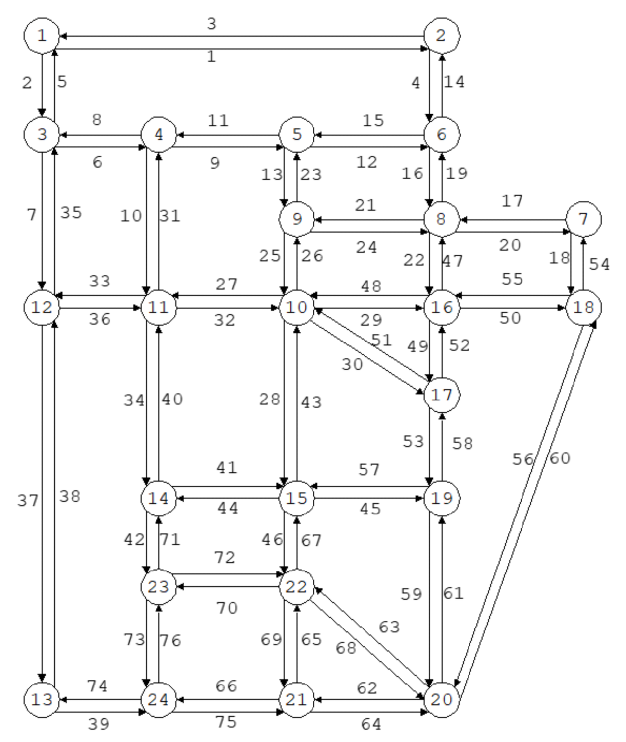
In this study, a simulation model was applied to the Sioux Falls network (24 nodes, 76 links) to calculate emissions levels. Sioux Falls is a network based on a real road network and has been widely used in existing studies as a simulation testbed for experimenting with newly constructed traffic models. The Sioux Falls network has been used in many studies and is a good traffic equilibrium network for testing traffic models. As many studies have shown, there are several versions of Sioux Falls network data, which were verified and organized in Bar-Gera et al. [27]. The first study that appeared was Morok et al., (1973) [28], and subsequent studies also showed different results using different cost functions. The network used in this study used the data presented in Bar-Gera et al. [29]. The Sioux Falls network uses the traditional BPR function, with an alpha parameter of 0.1 and a beta parameter of 2 [30]. It is a good network for verifying data and models through traffic assignment problems.

However, not all real road situations can be applied, and dynamic situations were not considered. In a recent study, a dynamic situation was considered using the actual traffic volume measured using the network fundamental diagram (NFD) [31], but the Sioux Falls network is a virtual network. Therefore, it was assumed that the driver knows all the road conditions and travels only on the shortest route in the network. There is a limitation for the stochastic model, in that it cannot be applied to all dynamic situations on the road that change every moment. However, dynamic situations are not considered in this study because the aim is to examine changes caused by policies. Therefore, traffic restriction according to the vehicle emission grades was applied to the link. Thus, in this study, this network (Figure 1) [29] was also selected to check the results of the model and accordingly proceeded with the analysis.

3. Methodology

3.1. Development of the Analysis Model

In this study, the aim was to calculate vehicle emissions based on a traffic demand model, which was created according to the road network. To do so, link volume and link speed were calculated according to the four-step traffic demand model. The four-step model includes trip generation, trip distribution, modal split, and trip assignment, through which an individual trip is assigned to the road network. This study employed the O-D data, and data of route distribution, modal split, and trip assignment were provided by previous simulation network studies. To select the final path, the route was assigned using the convex optimization algorithm.

Our study used the Frank–Wolfe [32] convex optimization algorithm to construct models that optimized traffic systems. The algorithm is based on the conditional gradient descent method, which determines the minimum value of this function when repeated operations are performed. It was applied to address the conditions of variable-demand traffic assignment in the middle of the course of primarily calculating the travel demand at the origin and destination, as well as the link volume [33].

To apply the algorithm, network data, O–D data, travel path, travel time, and parameters are required. For this model, we established these values using the R software program (v.4.1.0). In the model, the average travel speed throughout the link was set at 50 km/h to calculate the travel speed; however, this was not a limit, and travel speeds may be above 50 km/h or below 50 km/h on some links. Currently, the Seoul Municipal Government is implementing the “Safety Speed 5030” policy, which effects a downward adjustment of the maximum speed limit to 50 km/h on Seoul’s main roads and 30 km/h on other roads to ensure the safety of pedestrians.

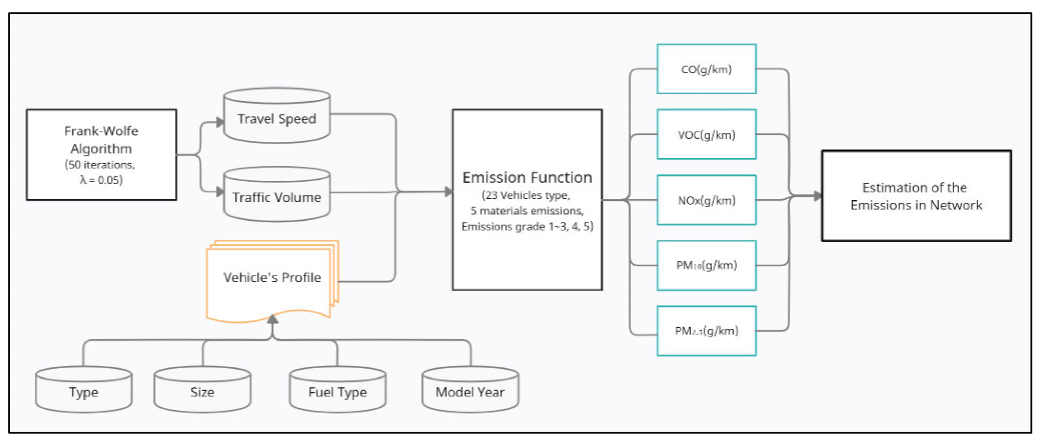
In this study, we applied 0.05 as the Frank–Wolfe (FW) algorithm (λ) value, based on a study conducted by Hwang and Ouyang (2015) [34]. In the FW algorithm, the shortest path algorithm was used. Route selection considers minimum travel time, minimum monetary cost, minimum congestion, minimum energy consumption, maximum motorway, etc. [35]. The shortest route was selected as per the minimum travel time in this study. When conducting the analysis, we applied 50 as the number of iterations performed. The model was completed by combining the emission functional formula, i.e., Equation (1), which is commonly used to calculate vehicle emissions using the travel speed and travel volume as calculated using the Frank–Wolfe algorithm. The data flow chart is shown in Figure 2.

$$Total Emission{s}_{i,j,k,l}={{\displaystyle \sum }}_i{{\displaystyle \sum }}_j{{\displaystyle \sum }}_k{{\displaystyle \sum }}_{l}VK{T}_{i,j,k,l}\times E{F}_{i,j,k,l}$$

(1)

VKT: vehicle kilometers traveled; EF: emission function;

i: vehicle type, j: fuel, k: model year, l: emission product

3.2. Emission Function

The substances and the degree of exhaust gases emitted from a vehicle depend on the vehicle type and size, the specific fuel used, and the model year of the vehicle. Because of the large difference in the amount of emissions produced by each characteristic, significant differences were observed when including/excluding these characteristics. As such, the vehicle exhaust-gas calculation method of the National Air Pollutants Emission Service [36] was applied. The advantage of using this method is that the varying amount of substances emitted based on the vehicle’s travel speed can be considered, and the total emissions can be determined by considering the traffic volume of the relevant link. It also has the advantage of determining more accurate emissions by considering the variable substance amounts emitted according to the vehicle type, model year, and the specific fuel used. Because the vehicle grade is classified by the vehicle’s model year, diesel vehicles registered before 2006 are classified into Grade 4, and diesel vehicles registered before are classified into Grade 5 [36]. The emission functions are shown in

Table A1. Emission function (National Institute of Environmental Research of Korea, 2016).

Size	Vehicle Type	Product	Fuel	Grade	ConnexPoint(km/h)	Function (V < Conxpoint)	Function (V ≥ Conxpoint)
small	car	CO	gasoline	1~3	N.A.	0.0001*V^(2)−0.0071*V + 0.2245	N.A.
	car	CO	diesel	1~3	N.A.	0.5775*V^(−0.7524)V	N.A.
	car	CO	LPG	1~3	N.A.	39.362*V^(−1.0085)V	N.A.
	car	VOC	gasoline	1~3	65.4	0.0633*V^(−1.0484)V	0.00000132*V^(2)−0.000188*V + 0.0077
	car	VOC	diesel	1~3	N.A.	0.0825*V^(−0.6848)V	N.A.
	car	VOC	LPG	1~3	N.A.	2.8981*V^(−1.3927)V	N.A.
	car	NOx	gasoline	1~3	N.A.	−0.0000035*V^(2)V + 0.0112	N.A.
	car	NOx	diesel	1~3	65.4	1.1849*V^(−0.5476)V	−0.000002*V^(2)V−0.011
	car	NOx	LPG	1~3	N.A.	1.8419*V^(−0.7864)V	N.A.
	car	PM10	diesel	1~3	N.A.	0.042*V^(−0.342)V	N.A.
	car	PM2.5	diesel	1~3	65	0.03864*V^(−0.342)V	0.042*V^(−0.342)V
	special	CO	diesel	1~3	N.A.	1.2211*V^(−0.6083)V	N.A.
	special	VOC	diesel	1~3	N.A.	0.1224*V^(−0.5684)V	N.A.
	special	NOx	diesel	1~3	65	2.0832*V^(−0.6485)V	−0.00003*V^(2)V−0.1339
	special	PM10	diesel	1~3	N.A.	0.1759*V^(−0.5357)V	N.A.
	special	PM2.5	diesel	1~3	65	0.161828*V^(−0.5357)V	0.1759*V^(−0.5357)V
	truck	CO	diesel	1~3	N.A.	1.2211*V^(−0.6083)V	N.A.
	truck	VOC	diesel	1~3	N.A.	1.2211*V^(−0.5684)V	N.A.
	truck	NOx	diesel	1~3	65	2.0832*V^(−0.6485)V	−0.00003*V^(2)V−0.1339
	truck	PM10	diesel	1~3	N.A.	0.1759*V^(−0.5357)V	N.A.
	truck	PM2.5	diesel	1~3	65	0.161828*V^(−0.5357)V	0.1759*V^(−0.5357)V
	van	CO	diesel	1~3	65.4	4.222*V^(−1.4035)V	0.01166*V^(0.0922)V
	van	VOC	diesel	1~3	N.A.	0.829*V^(−1.0961)V	N.A.
	van	NOx	diesel	1~3	65.4	2.6053*V^(−0.2645)V	0.0349*V^(0.7596)V
	van	PM10	diesel	1~3	N.A.	0.3111*V^(−0.5125)V	N.A.
	van	PM2.5	diesel	1~3	65.4	0.286212*V^(−0.5125)V	0.3111*V^(−0.5125)V
	car	CO	gasoline	4~5	N.A.	0.0001*V^(2)−0.0071*V + 0.2245	N.A.
	car	CO	diesel	4~5	N.A.	5.9672*V^(−0.9534)V	N.A.
	car	CO	LPG	4~5	N.A.	39.362*V^(−1.0085)V	N.A.
	car	VOC	gasoline	4~5	65	0.0633*V^(−1.0484)V	0.00000132*V^(2)−0.000188*V + 0.0077
	car	VOC	diesel	4~5	N.A.	0.6523*V^(−1.0167)V	N.A.
	car	VOC	LPG	4~5	N.A.	2.8981*V^(−1.3927)V	N.A.
	car	NOx	gasoline	4~5	N.A.	−0.0000035*V^(2)V + 0.0112	N.A.
	car	NOx	diesel	4~5	65	6.5209*V^(−0.6162)V	0.0001*V^(−0.0141)V + 0.908
	car	NOx	LPG	4~5	N.A.	1.8419*V^(−0.7864)V	N.A.
	car	PM10	diesel	4~5	65	0.3861*V^(−0.5093)V	−0.00001*V^(2)V−0.0618
	car	PM2.5	diesel	4~5	65	0.355212*V^(−0.5093)V	−0.00001*V^(2)V−0.0618
	special	CO	diesel	4~5	N.A.	4.5854*V^(−0.3613)V	N.A.
	special	VOC	diesel	4~5	N.A.	0.484*V^(−0.2756)V	N.A.
	special	NOx	diesel	4~5	65	11.788*V^(−0.6075)V	−0.0006*V^(2)V−3.6012
	special	PM10	diesel	4~5	N.A.	0.8117*V^(−0.4071)V	N.A.
	special	PM2.5	diesel	4~5	N.A.	0.746764*V^(−0.4071)V	N.A.
	truck	CO	diesel	4~5	N.A.	4.5854*V^(−0.3613)V	N.A.
	truck	VOC	diesel	4~5	N.A.	0.484*V^(−0.2756)V	N.A.
	truck	NOx	diesel	4~5	65	11.788*V^(−0.6075)V	−0.0006*V^(2)V + 3.6012
	truck	PM10	diesel	4~5	N.A.	0.8117*V^(−0.4071)V	N.A.
	truck	PM2.5	diesel	4~5	N.A.	0.746764*V^(−0.4071)V	N.A.
	van	CO	diesel	4~5	65	3.4539*V^(−0.4266)V	0.0051*V^(0.2212)V
	van	VOC	diesel	4~5	N.A.	0.9835*V^(−0.5096)V	N.A.
	van	NOx	diesel	4~5	65	8.415*V^(−0.5094)V	0.0004*V^(2)−0.0561*V + 2.891
	van	PM10	diesel	4~5	N.A.	1.1412*V^(−0.4324)V	N.A.
	van	PM2.5	diesel	4~5	N.A.	1.049904*V^(−0.4324)V	N.A.
mid	car	CO	gasoline	1~3	N.A.	0.0000229*V^(2)−0.00163*V + 0.0583	N.A.
	car	CO	diesel	1~3	N.A.	0.5414*V^(−0.7524)V	N.A.
	car	CO	LPG	1~3	N.A.	73.022*V^(−1.2078)V	N.A.
	car	VOC	gasoline	1~3	65	0.0633*V^(−1.0484)V	0.00000132*V^(2)−0.000188*V + 0.0077
	car	VOC	diesel	1~3	N.A.	0.0927*V^(−0.6848)V	N.A.
	car	VOC	LPG	1~3	N.A.	4.4166*V^(−1.5356)V	N.A.
	car	NOx	gasoline	1~3	N.A.	−0.0000035*V^(2)V + 0.0112	N.A.
	car	NOx	diesel	1~3	65	1.1281*V^(−0.5476)V	−0.000002*V^(2)V−0.0105
	car	NOx	LPG	1~3	N.A.	2.028*V^(−0.7978)V	N.A.
	car	PM10	diesel	1~3	N.A.	0.0396*V^(−0.342)V	N.A.
	car	PM2.5	diesel	1~3	N.A.	0.036432*V^(−0.342)V	N.A.
	special	CO	diesel	1~3	N.A.	4.5201*V^(−0.7279)V	N.A.
	special	VOC	diesel	1~3	N.A.	1.6826*V^(−0.8045)V	N.A.
	special	NOx	diesel	1~3	64.7	17.2485*V^(−0.404)V	1.1797*V^(0.2308)V
	special	PM10	diesel	1~3	64.7	0.0469*V^(−0.4674)V	0.000168*V^(1)V−0.00516
	special	PM2.5	diesel	1~3	64.7	0.043148*V^(−0.4674)V	0.000168*V^(1)V−0.00516
	truck	CO	diesel	1~3	N.A.	4.5201*V^(−0.7279)V	N.A.
	truck	VOC	diesel	1~3	N.A.	1.6826*V^(−0.8045)V	N.A.
	truck	NOx	diesel	1~3	64.7	17.2485*V^(−0.404)V	1.1797*V^(0.2308)V
	truck	PM10	diesel	1~3	64.7	0.0469*V^(−0.4674)V	0.000168*V^(1)V−0.00516
	truck	PM2.5	diesel	1~3	64.7	0.043148*V^(−0.4674)V	0.000168*V^(1)V−0.00516
	van	CO	diesel	1~3	N.A.	16.378*V^(−0.534)V	N.A.
	van	VOC	diesel	1~3	N.A.	5.8477*V^(−0.5466)V	N.A.
	van	NOx	diesel	1~3	80	25.436*V^(−0.4656)V	0.0008*V^(2)−0.0482*V + 1.8424
	van	PM10	diesel	1~3	N.A.	1.0457*V^(−0.4527)V	N.A.
	van	PM2.5	diesel	1~3	N.A.	0.962044*V^(−0.4527)V	N.A.
	car	CO	gasoline	4~5	N.A.	0.0000229*V^(2)−0.00163*V + 0.0583	N.A.
	car	CO	diesel	4~5	N.A.	0.5414*V^(−0.7524)V	N.A.
	car	CO	LPG	4~5	N.A.	73.022*V^(−1.2078)V	N.A.
	car	VOC	gasoline	4~5	65.4	0.0633*V^(−1.0484)V	0.00000132*V^(2)−0.000188*V + 0.0077
	car	VOC	diesel	4~5	N.A.	0.0927*V^(−0.6848)V	N.A.
	car	VOC	LPG	4~5	N.A.	4.4166*V^(−1.5356)V	N.A.
	car	NOx	gasoline	4~5	N.A.	−0.0000035*V^(2)V + 0.0112	N.A.
	car	NOx	diesel	4~5	65.4	1.1281*V^(−0.5476)V	−0.000002*V^(2)V−0.0105
	car	NOx	LPG	4~5	N.A.	2.028*V^(−0.7978)V	N.A.
	car	PM10	diesel	4~5	65	0.3861*V^(−0.5093)V	−0.00001*V^(2)V−0.0618
	car	PM2.5	diesel	4~5	65	0.355212*V^(−0.5093)V	−0.0000092*V^(2)V−0.0618
	special	CO	diesel	4~5	N.A.	16.769*V^(−0.3772)V	N.A.
	special	VOC	diesel	4~5	N.A.	6.7755*V^(−0.5003)V	N.A.
	special	NOx	diesel	4~5	N.A.	24.915*V^(−0.3942)V	N.A.
	Special	PM10	Diesel	4~5	N.A..	3.6772*V^(−0.5514)V	N.A.
	Special	PM2.5	Diesel	4~5	N.A.	3.383024*V^(−0.5514)V	N.A.
	Truck	CO	Diesel	4~5	N.A.	16.769*V^(−0.3772)V	N.A.
	Truck	VOC	Diesel	4~5	N.A.	6.7755*V^(−0.5003)V	N.A.
	Truck	NOx	Diesel	4~5	N.A.	24.915*V^(−0.3942)V	N.A.
	Truck	PM10	Diesel	4~5	N.A.	3.6772*V^(−0.5514)V	N.A.
	Truck	PM2.5	Diesel	4~5	N.A.	3.383024*V^(−0.5514)V	N.A.
	Van	CO	Diesel	4~5	N.A.	32.55*V^(−0.4994)V	N.A.
	Van	VOC	Diesel	4~5	N.A.	15.753*V^(−0.5912)V	N.A.
	Van	NOx	Diesel	4~5	80	40.692*V^(−0.559)V	−0.0023*V^(2)V−23.59
	Van	PM10	Diesel	4~5	N.A.	5.4886*V^(−0.5911)V	N.A.
	Van	PM2.5	Diesel	4~5	N.A.	5.049512*V^(−0.5911)V	N.A.
Large	Car	CO	Gasoline	1~3	65.4	1.4082*V^(−0.7728)V	0.00008*V^(2)−0.0127*V + 0.5751
	Car	CO	Diesel	1~3	N.A.	0.7507*V^(−0.7524)V	N.A.
	Car	CO	LPG	1~3	N.A.	73.022*V^(−1.2078)V	N.A.
	Car	VOC	Gasoline	1~3	65.4	0.0633*V^(−1.0484)V	0.00000132*V^(2)−0.000188*V + 0.0077
	Car	VOC	Diesel	1~3	N.A.	0.1554*V^(−0.6848)V	N.A.
	Car	VOC	LPG	1~3	N.A.	4.4166*V^(−1.5356)V	N.A.
	Car	NOx	Gasoline	1~3	N.A.	−0.0000035*V^(2)V+0.0112	N.A.
	Car	NOx	Diesel	1~3	65	1.1281*V^(−0.5476)V	−0.000002*V^(2)V−0.0105
	Car	NOx	LPG	1~3	N.A.	2.028*V^(−0.7978)V	N.A.
	Car	PM10	Diesel	1~3	N.A.	0.0361*V^(−0.342)V	N.A.
	Car	PM2.5	Diesel	1~3	N.A.	0.033212*V^(−0.342)V	N.A.
	Special	CO	Diesel	1~3	N.A.	52.136*V^(−0.8618)V	N.A.
	Special	VOC	Diesel	1~3	N.A.	3.7878*V^(−0.5425)V	N.A.
	Special	NOx	Diesel	1~3	N.A.	107.5*V^(−0.5679)V	N.A.
	Special	PM10	Diesel	1~3	N.A.	2.6847*V^(−0.6112)V	N.A.
	Special	PM2.5	Diesel	1~3	N.A.	2.469924*V^(−0.6112)V	N.A.
	Truck	CO	Diesel	1~3	N.A.	52.136*V^(−0.8618)V	N.A.
	Truck	VOC	Diesel	1~3	N.A.	3.7878*V^(−0.5425)V	N.A.
	Truck	NOx	Diesel	1~3	N.A.	107.5*V^(−0.5679)V	N.A.
	Truck	PM10	Diesel	1~3	N.A.	2.6847*V^(−0.6112)V	N.A.
	Truck	PM2.5	Diesel	1~3	N.A.	2.469924*V^(−0.6112)V	N.A.
	Van	CO	Diesel	1~3	N.A.	8.3966*V^(−0.8759)V	N.A.
	Van	VOC	Diesel	1~3	N.A.	1.2191*V^(−0.5266)V	N.A.
	Van	NOx	Diesel	1~3	N.A.	40.9398*V^(−0.5611)V	N.A.
	Van	PM10	Diesel	1~3	80	0.2986*V^(−0.5711)V	0.0001*V^(1.2263)V
	Van	PM2.5	Diesel	1~3	80	0.274712*V^(−0.5711)V	0.0001*V^(1.2263)V
	Car	CO	Gasoline	4~5	65.4	1.4082*V^(−0.7728)V	0.00008*V^(2)−0.0127*V+0.5751
	Car	CO	Diesel	4~5	N.A.	5.9672*V^(−0.9534)V	N.A.
	Car	CO	LPG	4~5	N.A.	73.022*V^(−1.2078)V	N.A.
	Car	VOC	Gasoline	4~5	65.4	0.0633*V^(−1.0484)V	0.00000132*V^(2)−0.000188*V+0.0077
	Car	VOC	Diesel	4~5	N.A.	0.6523*V^(−1.0167)V	N.A.
	Car	VOC	LPG	4~5	N.A.	4.4166*V^(−1.5356)V	N.A.
	Car	NOx	Gasoline	4~5	N.A.	−0.0000035*V^(2)V+0.0112	N.A.
	Car	NOx	Diesel	4~5	65	6.5209*V^(−0.6162)V	0.0001*V^(2)−0.0141*V+0.908
	Car	NOx	LPG	4~5	N.A.	2.028*V^(−0.7978)V	N.A.
	Car	PM10	Diesel	4~5	65	0.3861*V^(−0.5093)V	−0.00001*V^(2)V−0.0618
	Car	PM2.5	Diesel	4~5	65	0.355212*V^(−0.5093)V	−0.0000092*V^(2)V−0.0618
	Special	CO	Diesel	4~5	N.A.	30.402*V^(−0.4685)V	N.A.
	Special	VOC	Diesel	4~5	N.A.	15.75*V^(−0.582)V	N.A.
	Special	NOx	Diesel	4~5	N.A.	117.49*V^(−0.365)V	N.A.
	Special	PM10	Diesel	4~5	N.A.	7.6212*V^(−0.4183)V	N.A.
	Special	PM2.5	Diesel	4~5	N.A.	7.011504*V^(−0.4183)V	N.A.
	Truck	CO	Diesel	4~5	N.A.	30.402*V^(−0.4685)V	N.A.
	Truck	VOC	Diesel	4~5	N.A.	15.75*V^(−0.582)V	N.A.
	Truck	NOx	Diesel	4~5	N.A.	117.49*V^(−0.365)V	N.A.
	Truck	PM10	Diesel	4~5	N.A.	7.6212*V^(−0.4183)V	N.A.
	Truck	PM2.5	Diesel	4~5	N.A.	7.011504*V^(−0.4183)V	N.A.
	Van	CO	Diesel	4~5	N.A.	28.205*V^(−0.5337)V	N.A.
	Van	VOC	Diesel	4~5	N.A.	6.1146*V^(−0.4979)V	N.A.
	Van	NOx	Diesel	4~5	N.A.	41.346*V^(−0.3645)V	N.A.
	Van	PM10	Diesel	4~5	N.A.	5.2158*V^(−0.5048)V	N.A.
	Van	PM2.5	Diesel	4~5	80	4.798536*V^(−0.5048)V	4.798536*V^(−0.5048)V
Light	Car	CO	Gasoline	1~3	45	4.4952*V^(−0.8461)V	−0.0001*V^(2)V−0.5701
	Car	CO	Diesel	1~3	N.A.	0.5775*V^(−0.7524)V	N.A.
	Car	CO	LPG	1~3	45	8.9904*V^(−0.8461)V	−0.0002*V^(2)V−1.1403
	Car	VOC	Gasoline	1~3	N.A.	0.2958*V^(−0.783)V	N.A.
	Car	VOC	Diesel	1~3	N.A.	0.0825*V^(−0.6848)V	N.A.
	Car	VOC	LPG	1~3	N.A.	0.3549*V^(−0.783)V	N.A.
	Car	NOx	Gasoline	1~3	N.A.	0.4819*V^(−0.9198)V	N.A.
	Car	NOx	Diesel	1~3	45	1.1849*V^(−0.5476)V	−0.000002*V^(2)V−0.011
	Car	NOx	LPG	1~3	N.A.	0.7228*V^(−0.9198)V	N.A.
	Car	PM10	Diesel	1~3	N.A.	0.042*V^(−0.342)V	N.A.
	Car	PM2.5	Diesel	1~3	N.A.	0.03864*V^(−0.342)V	0.042*V^(−0.342)V
	Truck	CO	Gasoline	1~3	45	4.4952*V^(−0.8461)V	−0.0001*V^(2)V−0.5701
	Truck	VOC	Gasoline	1~3	N.A.	0.2958*V^(−0.3236)V	N.A.
	Truck	NOx	Gasoline	1~3	N.A.	0.4819*V^(−0.9198)V	N.A.
	Van	CO	Gasoline	1~3	45	4.4952*V^(−1.4035)V	0.01166*V^(0.0922)V
	Van	VOC	Gasoline	1~3	N.A.	0.2958*V^(−0.783)V	N.A.
	Van	NOx	Gasoline	1~3	N.A.	0.4819*V^(−0.9198)V	N.A.
	Car	CO	Gasoline	4~5	45	4.4952*V^(−0.8461)V	−0.0001*V^(2)V−0.5701
	Car	CO	Diesel	4~5	N.A.	0.7392*V^(−0.7524)V	N.A.
	Car	CO	LPG	4~5	45	8.9904*V^(−0.8461)V	−0.0002*V^(2)V−1.1403
	Van	CO	Gasoline	4~5	45	4.4952*V^(−1.4035)V	0.01166*V^(0.0922)V
	Truck	CO	Gasoline	4~5	45	4.4952*V^(−0.8461)V	−0.0001*V^(2)V−0.5701
	Car	VOC	Gasoline	4~5	N.A.	0.2958*V^(−0.783)V	N.A.
	Car	VOC	Diesel	4~5	N.A.	0.0989*V^(−0.6848)V	N.A.
	Car	VOC	LPG	4~5	N.A.	0.3549*V^(−0.783)V	N.A.
	Van	VOC	Gasoline	4~5	N.A.	0.2958*V^(−0.783)V	N.A.
	Truck	VOC	Gasoline	4~5	N.A.	0.2958*V^(−0.3236)V	N.A.
	Car	NOx	Gasoline	4~5	N.A.	0.4819*V^(−0.9198)V	N.A.
	Car	NOx	Diesel	4~5	65	2.3699*V^(−0.5476)V	−0.000004*V^(2)V−0.0219
	Car	NOx	LPG	4~5	N.A.	0.7228*V^(−0.9198)V	N.A.
	Van	NOx	Gasoline	4~5	N.A.	0.4819*V^(−0.9198)V	N.A.
	Truck	NOx	Gasoline	4~5	N.A.	0.4819*V^(−0.9198)V	N.A.
	Car	PM10	Diesel	4~5	N.A.	0.0839*V^(−0.342)V	N.A.
	Car	PM2.5	Diesel	4~5	N.A.	0.077188*V^(−0.342)V	N.A.

(Appendix A).

4. Results

4.1. Emission Function and Vehicle Properties

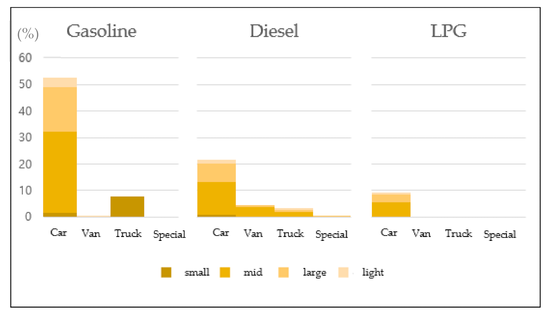
The emission function used by the National Institute of Environmental Research of Korea is categorized by vehicle type, pollutant substance, and vehicle model year. We considered the degree to which each function represented emissions differences before applying it to the model we created. First, the vehicle property data used in this study were derived from vehicle registration status reports in December 2020 provided by the Korean Ministry of Land, Infrastructure, and Transport [37]. Using these data, the proportion of registered vehicles was identified by type, fuel, size, and model year. According to the Korean Ministry of Enivronment, the size was determined by the engine displacement. Light vehicles are smaller than 1000 cc, and small vehicles are between 1000 cc and 1600 cc. Mid-size vehicles are between 1600 cc and 2000 cc, and big (large and extra-large size) vehicles are classified as above 2000 cc. Although large and extra-large vehicles have been distinguished, they are considered as one function in the emission function. When allocated by vehicle type, size, and fuel type, the results were the same as shown in Figure 3, i.e., classified into 23 different types. Therefore, 69 types were considered in emissions Grade 1–3 vehicles and for Grade 4 and Grade 5 vehicles.

The classification of vehicle classes is shown in

Table 2. Korea’s vehicle emissions grading standard.

Grade	Type of Vehicle
	Electric/Hydrogen Vehicle	Gasoline/LPG Vehicle (Including Hybrid)	Diesel Vehicle (Including Hybrid)
1–3	All Types of Vehicles	2006–2016 model year	2009–2014 model year
4	N/A	2002 model year	2006 model year
5		2000 model year	2002 model year

. Grade 1–3 vehicles consist of all types of electric vehicles, 2006–2016 model year of gasoline and liquefied petroleum gas (LPG) vehicles’ standard, and 2009–2014 model year of diesel vehicles’ standard. Grade 4 vehicles consist of 2002 model year of gasoline and LPG vehicle’s standard and 2006 model year of diesel vehicle’s standard. Grade 5 vehicles consist of 2000 model year of gasoline and LPG vehicle’s standard and 2002 model year of diesel vehicle’s standard [38]. In terms of emissions, three substances were applied, i.e., carbon monoxide (CO), VOCs, and NOx because all vehicles emitted these. Particulate matter PM₁₀ and PM_2.5 were considered only for diesel vehicles. (Figure 3).

The results of applying emission functions to the categorized vehicle properties are shown in Figure 4. Of the total proportion of vehicles, the ratio of passenger cars using gasoline was the highest, followed by the ratio of diesel passenger cars. Gasoline-powered cargo vehicles were all found to be small vehicles; other vehicles were found to use diesel oil. Liquid petroleum gas (LPG) vehicles were all identified as passenger cars (see Figure 4).

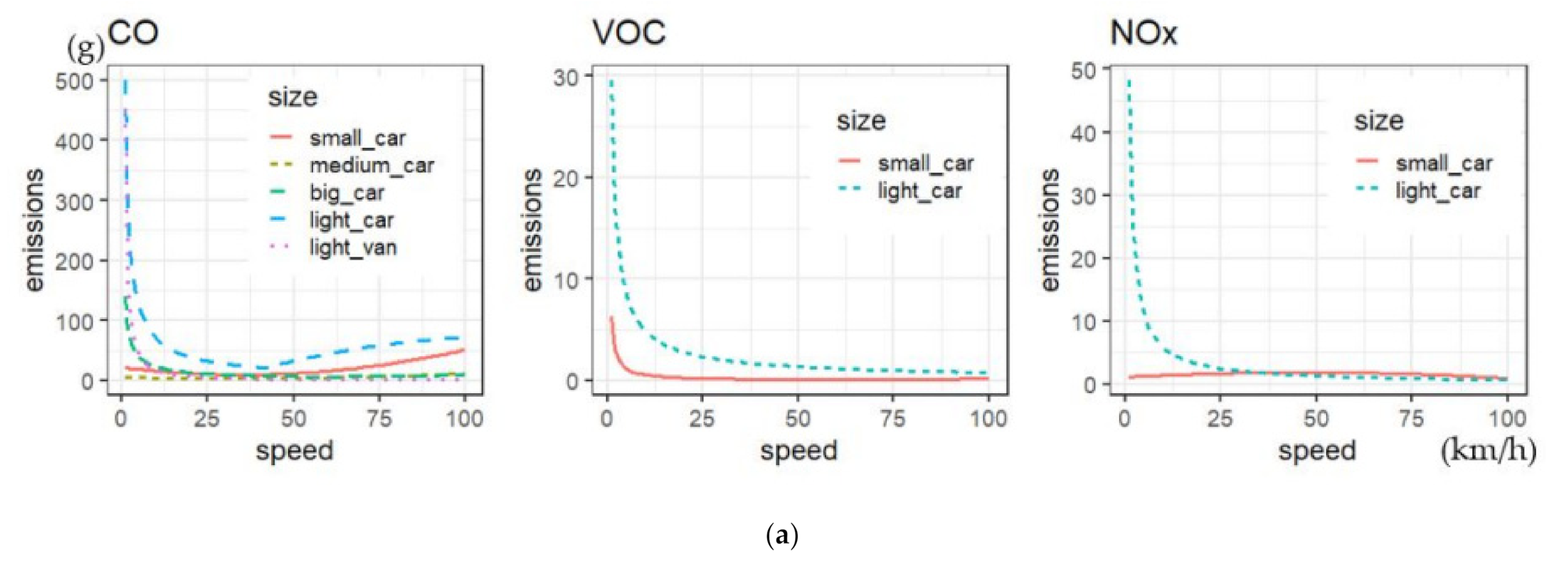
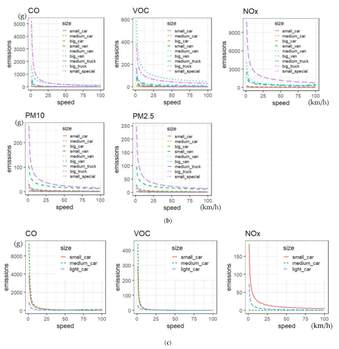
By applying the emission function to each vehicle’s properties, the results for each emission substance are shown in Figure 5a–c, and the result of each emission function was classified according to the fuel used in the vehicle. The number of vehicles applied to the emission function was 1000, and the maximum speed was set at 100 km/h. The overall function shared the characteristic in which the closer the travel speed was to zero, the higher the emissions; this indicated that an increase in travel speed reduced emissions. The total emissions were of the highest value among vehicles using diesel oil, of which the CO and NOx emissions were significant. It is explained that the reason why the application of vehicle restriction policy is limited to diesel vehicles is because the amount of matter emitted is larger compared to other fuel types.

4.2. The Results of Emission Calculation Using the Study Model

Considering the vehicles within each scenario, analysis was conducted by applying a previously established travel model. When the traffic on the network decreased by limiting the number of vehicles, the travel speed and traffic volume for each link were affected. A finalized emission calculation model was developed by linking previously established traffic demand model and the emission function, and scenario analysis was conducted based on the following road network.

In Scenario 1, the proportion of reduced vehicles was 97.2%, which included a 2.8% decrease in older diesel vehicles, resulting in an increase in the average travel speed for each link by 5.46 km/h. In Scenario 2, compared with Scenario 0, 5.5% of Grades 4 and 5 diesel vehicles were restricted, and the average travel speed increased by 8.33 km/h. These results indicated that the traffic volume per link had decreased due to the vehicle grade-based restriction policy, which increased the vehicle travel speed. Furthermore, decreasing traffic volume and increasing travel speeds reduced vehicle emissions; this change in traffic conditions was also considered in the analysis using the route model (

Table 3. Changes in vehicle proportion and the average travel speed for each scenario.

Division	Vehicle Proportion (%)	Average Travel Speed (km/h)
Scenario 0 (with no restriction)	100	29.56
Scenario 1 (grade 5 diesel vehicle restricted)	97.2	34.90
Scenario 2 (grade 4/5 diesel vehicle restricted)	94.5	37.89

).

After calculating the emissions for each scenario, overall emissions were found to decrease as the situation progressed from Scenario 0 to Scenario 2. The following results were derived by subdividing the outcomes of the analysis by vehicle type, emission substance, vehicle grade, and fuel.

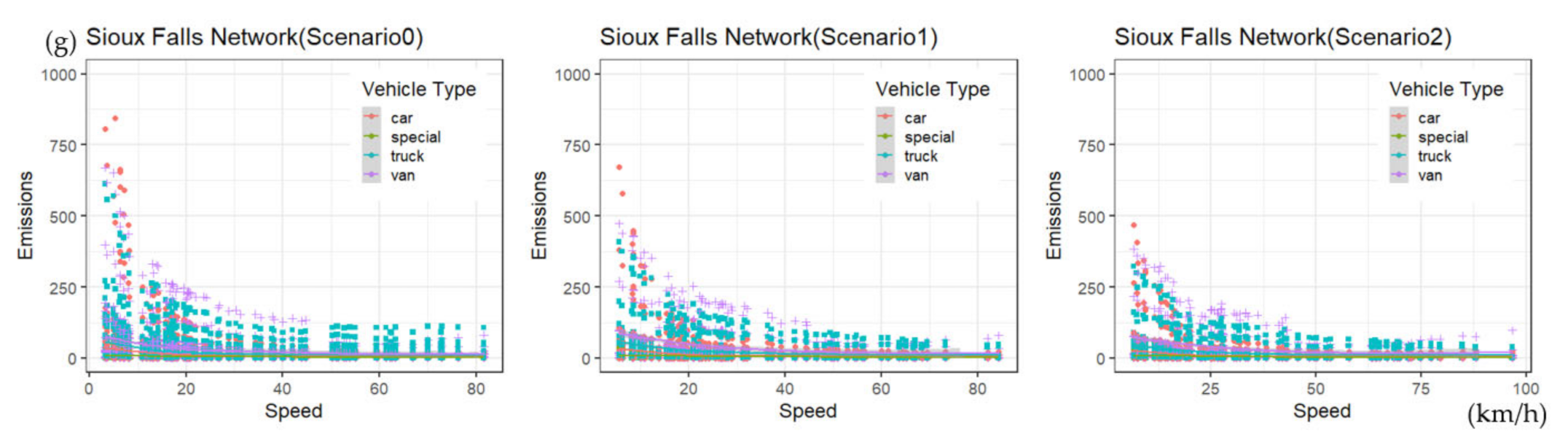
First, the emission results according to vehicle type showed high emissions in the low-speed range (0–20 km/h), and passenger cars accounted for the highest emission levels. Conversely, in the high-speed range (60–80 km/h), high emission levels were presented in the order of cargo vehicles, vans, and special vehicles, and these vehicles were found to be primarily diesel-powered. As we progressed to Scenarios 1 and 2, we found that the emissions observed in the low-speed range decreased significantly; the cargo vehicle emissions in Scenario 0 also decreased significantly (Figure 6).

The emissions by vehicle type, based on the grade for each scenario, are shown in

Table 4. Emissions by vehicle type for each individual scenario.

Classification	Grade	Vehicle Type (g/km)				Total Emissions (g/km)
		Car	Van	Truck	Special
scenario 0	1~5	47,513.6	47,531.2	51,921.3	2618.2	149,584.3
scenario 1	1~4	28,644.8	26,667.1	25,654.7	1683.6	84,357.1
	5	1701.7	5.1	0.0	0.0
	Total	30,346.5	26,672.2	25,654.7	1683.6	-
scenario 2	1~3	23,576.8	23,169.9	21,871.6	1501.2	73,614.7
	4~5	3489.0	6.2	0.0	0.0
	Total	27,065.8	23,176.1	21,871.6	1501.2	-

. In Scenario 0, the total emissions were 149,584.3 g/km; the total emissions of trucks were the highest among each type of vehicle; however, the emissions of passenger cars and vans were found to be similar. The total emissions result for Scenario 1 was 84,357.1 g/k, which was 43.6% lower compared with Scenario 0. Notably, when Grade 5 diesel vehicles were restricted, the emissions of Grade 1–4 vehicles also decreased. The total emissions in Scenario 2 were 73,614.7 g/km, which did not decrease significantly compared to the decrease in Scenario 1 (Table 4).

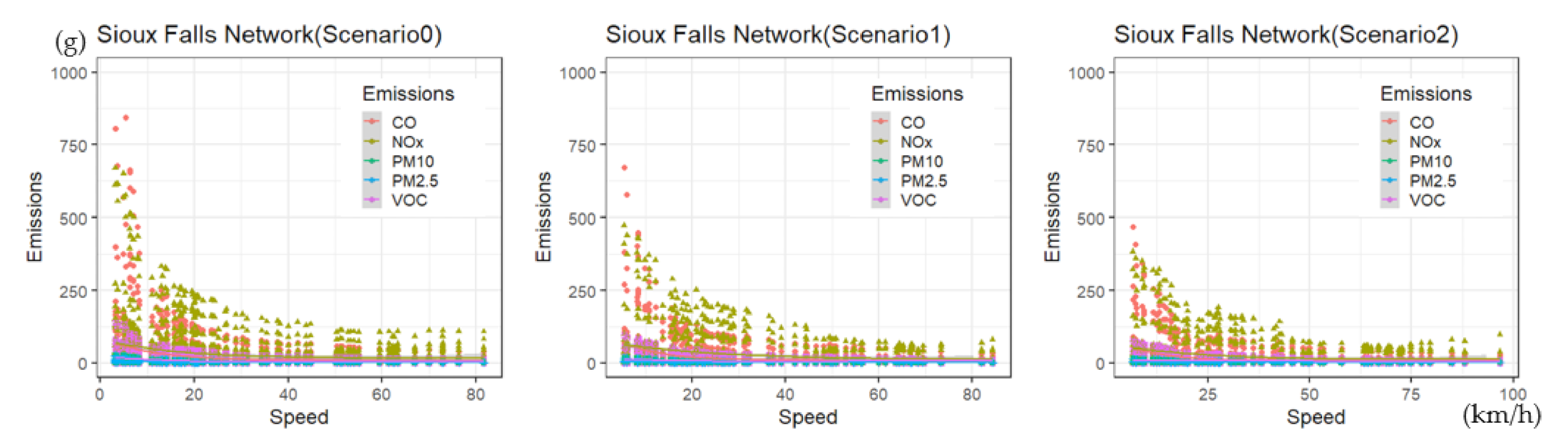
By substance, CO and NOx ranked the highest among the total emissions. As previously observed in the emission function, a significant percentage of these emissions was assumed to be derived from low-speed diesel vehicles. Passenger vehicles powered by LPG also generated a significant level of emissions. Many VOCs were emitted, followed in amount by PM₁₀ and PM_2.5. In the case of fine dust, we assumed that relatively small amounts were emitted compared with the total emissions because only the emissions of diesel vehicles were considered (Figure 7).

Considering the emissions by substance and according to vehicle grade, a noticeable decrease was observed in NOx, which had the highest emissions levels in Scenario 0. However, in Scenario 2, higher emissions of CO, VOCs, and NOx were observed for Grade 4–5 vehicles compared with Scenario 0; this appeared to have been the result of changes in traffic flow, in which the limited number of vehicles varied by grade (

Table 5. Emissions by substance for each scenario.

Classification	Grade	Product (g/km)					Total Emissions (g/km)
		CO	VOC	NOx	PM10	PM2.5
scenario 0	1~5	60,298.3	10,447.3	72,287.9	3403.1	3147.7	149,584.3
scenario 1	1~4	32,582.4	5552.6	41,807.3	1400.1	1307.9	84,357.1
	5	1496.8	47.6	162.4	0.0	0.0
	Total	34,079.2	5600.2	41,969.7	1400.1	1307.9	-
scenario 2	1~3	26,976.3	4700.1	36,116.9	1202.3	1123.8	73,614.7
	4~5	3058.7	93.5	343.0	0.0	0.0
	Total	30,035.0	4793.6	36,459.9	1202.3	1123.8	-

).

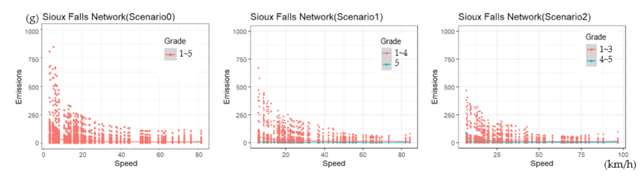
When reviewing by grade according to vehicle model year, the emissions from Grade 5 vehicles, which appeared in Scenario 0, were found to gradually disappear as we progressed into Scenarios 1 and 2. From these results, it was confirmed that the lower-grade vehicle restriction policy had an effect on reduction in emissions levels. Emissions in the low-speed range of Scenario 2 were reduced by 40% compared to the low-speed range of Scenario 0; however, some of the vehicles that moved at a speed of approximately 100 km/h due to an increased travel speed showed slightly increased emissions. However, given the degree of emissions reduced at low speeds, the level of emissions decreased overall (Figure 8).

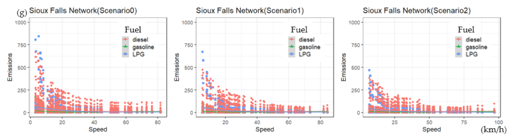
In terms of fuel type, the emissions levels of diesel-fueled vehicles were high overall, and LPG vehicle emissions were noticeably high in the low-speed range. It is estimated that this is because the emission function of LPG vehicles is designed to increase rapidly compared to other functions when the speed is 0. Therefore, if the average travel speed by link increased due to the restriction on older diesel vehicles, we might assume that the emissions of LPG vehicles will decrease. However, since LPG passenger vehicles accounted for a considerable portion of cars in the city, we believe that additional measures should be enforced against LPG vehicles, similar to those for older diesel vehicles (Figure 9).

When considering emission levels by fuel type and according to vehicle grade, diesel-fueled vehicles reflected the highest emissions in Scenario 0. Specifically, the emissions of Grade 5 diesel-fueled vehicles accounted for 22% of the total emissions. In Scenarios 1 and 2, where vehicle restriction was in place, emissions from diesel-fueled vehicles were found to have been reduced by 47% and 54%, respectively, compared with Scenario 0 (

Table 6. Emissions based on fuel type for each scenario.

Classification	Grade	Fuel (g/km)			Total Emissions (g/km)
		Gasoline	Diesel	LPG
scenario0	1~5	9084.0	112,375.3	28,125.0	149,584.3
scenario1	1~3	6620.8	60,447.8	15,581.6	84,357.1
	4~5	495.0	0.0	1211.9
	Total	7115.8	60,447.8	16,793.5	-
scenario2	1~3	5696.0	52,004.3	12,419.1	73,614.7
	4~5	1066.0	0.0	2429.3
	Total	6762.0	52,004.3	14,848.4	-

).

5. Discussions

Using our traffic model, we were able to calculate the emissions from each vehicle accurately by considering the changes in traffic flow. Importantly, we were able to observe the extent to which the grade-based vehicle restriction policy contributes to a reduction in emissions in specific scenarios. Furthermore, we identified the cause by classifying based on vehicle type, emitted substance, vehicle grade, and fuel type.

Although other studies reported a change in travel speed due to traffic policy [8], in this study, the average travel speed was found to increase due to vehicle restrictions. It was confirmed that the result directly leads to emission reduction when only the restriction policy according to the vehicle grade system is considered. Considering the characteristics of urban traffic, it appeared similar to the study results of Rodríguez et al., (2016) in terms of traffic congestion and low travel speed [11]. As shown in the results in this study, hybrid vehicles that use electricity at low speeds are expected to greatly contribute to the reduction in emissions. Considering the emissions by substance, it was confirmed that the changes in NOx and VOC vary greatly depending on the vehicle’s characteristics and circumstances, as observed by Osorio and Nanduri (2015) [12].

Based on these results, policymakers need to consider whether the current vehicle grading system is working properly. In particular, the Korean Ministry of Environment must measure vehicle emission reliably, and every vehicle owner must manage their vehicle well. In the same vein, the central government should support and regulate the conversion of old diesel vehicles to eco-friendly vehicles, particularly considering old trucks and special vehicles. In addition, the government needs to support the development of eco-friendly vehicle technology. The environmental organization must encourage the government and citizens through a campaign about switching to eco-friendly vehicles. Additionally, the City of Seoul, which already has a well-developed and extensive public transportation system that is eco-friendly, needs to encourage people to use public transportation more than private vehicles.

6. Conclusions

In this study, an emission calculation model that accounted for changes in traffic flow in conjunction with the emission function was constructed using a traffic demand model based on a simulation network. Based on this, the changes in emissions were examined for Scenarios 0, 1, and 2, which were based on the vehicle grade being restricted. The changes were examined according to vehicle type, the emitted substances, vehicle grade, and fuel type in Seoul, and the results were summarized to derive the following implications.

First, following the vehicle restriction policy being enforced, the emission reductions among passenger cars in the low-speed range (0–20 km/h) were the most significant, while those in the high-speed range (60–80 km/h) were significant for cargo trucks. The primary vehicles used in Seoul are passenger cars, and the city’s municipal government is currently implementing the “Safety Speed 5030” policy. Although enforcing vehicle speed-limiting policies promotes safety, the impact of these policies on air pollution due to exhaust emissions must be further examined.

Second, the recorded emissions were high in CO and NOx contents and were high in the case of LPG vehicles and diesel vehicles. Currently, the vehicle restriction policy is only implemented for diesel vehicles; other vehicles are graded but not subject to restrictions. Our analysis showed that the emissions of LPG vehicles were considerable compared with older diesel vehicles; therefore, we believe that some measures need to be taken against this.

Third, when more vehicles were restricted in a scenario, the overall reduction in emissions was greater. Accordingly, we found that the vehicle restriction policy appeared to be effective for improving air pollution.

Fourth, it was confirmed that the vehicle restriction policy not only reduced the emissions of diesel vehicles but also those of other vehicles. This means that easing traffic flows gave rise to smoother traffic flow in the city, which improved the travel speed and reduced the level of emissions. As such, we found that the air quality of the entire city could be improved by restricting the use of older diesel vehicles, which were the main source of urban air pollutants.

In conclusion, using the model derived in this study, we were able to identify the effects of the vehicle restriction policy while also considering traffic flow. Our results show that this restriction affected the emissions levels of diesel and other vehicles.

There are, however, some limitations to the current study’s results. First, the model only considered the travel speed by link; this gave rise to a limitation in which emissions due to acceleration/deceleration were not examined. Furthermore, new fuel energy types for hybrid cars, electric vehicles, and hydrogen cars were not considered. Our study was restricted to fuels used in existing internal combustion engine vehicles. In future research, it will be necessary to compare the results of applying this model to Seoul’s traffic network with emissions levels calculated considering the actual traffic volume and vehicles using various energy sources.

References

- WHO, World Health Organization. Air Pollution 2008. 2020. Available online: https://www.who.int/health-topics/air-pollution#tab=tab_1 (accessed on 20 July 2021).
- Kunkler, J.; Braun, M.; Kellner, F. Speed Limit Induced CO2 Reduction on Motorways: Enhancing Discussion Transparency through Data Enrichment of Road Networks. Sustainability 2021, 13, 395. [Google Scholar] [CrossRef]
- Gan, J.; Li, L.; Xiang, Q.; Ran, B. A Prediction Method of GHG Emissions for Urban Road Transportation Planning and Its Applications. Sustainability 2020, 12, 10251. [Google Scholar] [CrossRef]
- Korean Ministry of Environment. Available online: http://me.go.kr/home/web/main.do (accessed on 20 July 2021).
- DieselNet. Summary of Worldwide Engine and Vehicle Emission Standards. Available online: https://dieselnet.com/standards/ (accessed on 13 August 2021).
- Franco, V.; Kousoulidou, M.; Muntean, M.; Ntziachristos, L.; Hausberger, S.; Dilara, P. Road vehicle emission factors development: A review. Atmos. Environ. 2013, 70, 84–97. [Google Scholar] [CrossRef]
- Berkowicz, R.; Winther, M.; Ketzel, M. Traffic pollution modelling and emission data. Environ. Model. Softw. 2006, 21, 454–460. [Google Scholar] [CrossRef]
- Lv, J.; Zhang, Y. Effect of signal coordination on traffic emission. Transp. Res. Part D Transp. Environ. 2012, 17, 149–153. [Google Scholar] [CrossRef]
- Panis, L.I.; Broekx, S.; Liu, R. Modelling instantaneous traffic emission and the influence of traffic speed limits. Sci. Total Environ. 2006, 371, 270–285. [Google Scholar] [CrossRef]
- Hwang, H.; Song, C.K. Changes in air pollutant emissions from road vehicles due to autonomous driving technology: A conceptual modeling approach. Environ. Eng. Res. 2020, 25, 366–373. [Google Scholar] [CrossRef]
- Rodríguez, R.A.; Virguez, E.A.; Rodríguez, P.A.; Behrentz, E. Influence of driving patterns on vehicle emissions: A case study for Latin American cities. Transp. Res. Part D Transp. Environ. 2016, 43, 192–206. [Google Scholar] [CrossRef]
- Osorio, C.; Nanduri, K. Urban transportation emissions mitigation: Coupling high-resolution vehicular emissions and traffic models for traffic signal optimization. Transp. Res. Part B Methodol. 2015, 81, 520–538. [Google Scholar] [CrossRef]
- Cho, K.; Eom, M.; Kim, C.; Hong, Y.; Kim, C.; Han, Y. A Study on Estimation of Emission Factors and Emission Rates for Motor Vehicles. J. Korean Soc. Atmos. Environ. 1993, 9, 69–77. (In Korean) [Google Scholar]
- Zhu, W.X.; Zhang, J.Y. An original traffic additional emission model and numerical simulation on a signalized road. Phys. A Stat. Mech. Its Appl. 2017, 467, 107–119. [Google Scholar] [CrossRef]
- Kun, C.; Lei, Y.U. Microscopic traffic-emission simulation and case study for evaluation of traffic control strategies. J. Transp. Syst. Eng. Inf. Technol. 2007, 7, 93–99. [Google Scholar]
- Huang, C.; Tao, S.; Lou, S.; Hu, Q.; Wang, H.; Wang, Q.; Li, L.; Wang, H.; Liu, J.; Quan, Y.; et al. Evaluation of emission factors for light-duty gasoline vehicles based on chassis dynamometer and tunnel studies in Shanghai, China. Atmos. Environ. 2017, 169, 193–203. [Google Scholar] [CrossRef]
- Borge, R.; Lumbreras, J.; Pérez, J.; de la Paz, D.; Vedrenne, M.; de Andrés, J.M.; Rodríguez, M.E. Emission inventories and modeling requirements for the development of air quality plans. Application to Madrid (Spain). Sci. Total Environ. 2014, 466, 809–819. [Google Scholar] [CrossRef] [Green Version]
- Outapa, P.; Thepanondh, S.; Kondo, A.; Pala-En, N. Development of air pollutant emission factors under real-world truck driving cycle. Int. J. Sustain. Transp. 2018, 12, 432–440. [Google Scholar] [CrossRef]
- Song, X.; Hao, Y. Research on the Vehicle Emission Characteristics and Its Prevention and Control Strategy in the Central Plains Urban Agglomeration, China. Sustainability 2021, 13, 1119. [Google Scholar] [CrossRef]
- Han, D.; Lee, Y.; Chang, H. A Study of Calculation Methodology of Vehicle Emissions based on Driver Speed and Acceleration Behavior. J. Korean Soc. Transp. 2011, 29, 107–120. (In Korean) [Google Scholar]
- Taljegard, M.; Thorson, L.; Odenberger, M.; Johnsson, F. Large-scale implementation of electric road systems: Associated costs and the impact on CO2 emissions. Int. J. Sustain. Transp. 2020, 14, 606–619. [Google Scholar] [CrossRef] [Green Version]
- Roukounakis, N.; Valkouma, E.; Giama, E.; Gerasopoulos, E. The development of a carbon footprint model for the calculation of GHG emissions from highways: The case of Egnatia Odos in Greece. Int. J. Sustain. Transp. 2020, 14, 74–83. [Google Scholar] [CrossRef]
- Leblanc, L.J. An algorithm for the discrete network design problem. Transp. Sci. 1975, 9, 183–199. [Google Scholar] [CrossRef]
- LeBlanc, L.J.; Morlok, E.K.; Pierskalla, W.P. An efficient approach to solving the road network equilibrium traffic assignment problem. Transp. Res. 1975, 9, 309–318. [Google Scholar] [CrossRef]
- Suwansirikul, C.; Friesz, T.L.; Tobin, R.L. Equilibrium decomposed optimization: A heuristic for the continuous equilibrium network design problem. Transp. Sci. 1987, 40, 540–542. [Google Scholar] [CrossRef]
- Meng, Q.; Yang, H.; Bell, M.G.H. An equivalent continuously differentiable model and a locally convergent algorithm for the continuous network design problem. Transp. Res. Part B 2001, 35, 83–105. [Google Scholar] [CrossRef]
- Bar-Gera, H.; Hellman, F.; Patriksson, M. Computational precision of traffic equilibria sensitivities in automatic network design and road pricing. Procedia-Soc. Behav. Sci. 2013, 80, 41–60. [Google Scholar] [CrossRef] [Green Version]
- Morlok, E.K.; Schofer, J.L.; Pierskalla, W.P.; Marsten, R.E.; Agarwal, S.K.; Stoner, J.W.; Edwards, J.L.; LeBlanc, L.J.; Spacek, D.T. Development and Application of a Highway Network Design Model: Transportation Center Research Report. In Environmental Planning Branch, Federal Highway Administration; U.S. Department of Transportation Northwestern University: Evanston, IL, USA, 1973; Volume 2, Available online: https://www.scholars.northwestern.edu/en/publications/development-and-application-of-a-highway-network-design-model-tra (accessed on 24 August 2021).
- Bar-Gera, H. Transportation network Test Problems. 2001. Available online: https://www.bgu.ac.il/~bargera/tntp/ (accessed on 25 July 2021).
- Ukkusuri, S.V.; Yushimito, W.F. A methodology to assess the criticality of highway transportation networks. J. Transp. Secur. 2009, 2, 29–46. [Google Scholar] [CrossRef]
- Alonso, B.; Pòrtilla, Á.I.; Musolino, G.; Rindone, C.; Vitetta, A. Network Fundamental Diagram (NFD) and traffic signal control: First empirical evidences from the city of Santander. Transp. Res. Procedia 2017, 27, 27–34. [Google Scholar] [CrossRef]
- Frank, M.; Wolfe, P. An algorithm for quadratic programming. Nav. Res. Logist 1956, 3, 95–110. [Google Scholar] [CrossRef]
- Xie, C.; Waller, S.T. Stochastic traffic assignment, Lagrangian dual, and unconstrained convex optimization. Transp. Res. Part B Methodol. 2012, 46, 1023–1042. [Google Scholar] [CrossRef]
- Hwang, T.; Ouyang, Y. Urban freight truck routing under stochastic congestion and emission considerations. Sustainability 2015, 7, 6610–6625. [Google Scholar] [CrossRef] [Green Version]
- Croce, A.I.; Musolino, G.; Rindone, C.; Vitetta, A. Route and Path Choices of Freight Vehicles: A Case Study with Floating Car Data. Sustainability 2020, 12, 8557. [Google Scholar] [CrossRef]
- National Institute of Environmental Research of Korea. Available online: https://nier.go.kr/NIER/kor/index.do (accessed on 29 July 2021).
- Korean Ministry of Land, Infrastructure and Transport. Total Registered Moter Vehicles 2020. Available online: http://stat.molit.go.kr/portal/cate/statMetaView.do?hRsId=58&hFormId=&hDivEng=&month_yn= (accessed on 24 August 2021).
- Korean Ministry of Environment. Korean Ministry of Environment’s Vehicle Emission Grading Standard. Available online: https://emissiongrade.mecar.or.kr/www/ceg/cegCalcRule.do (accessed on 12 August 2021).
Figure 1.
Sioux Falls network [29].
Figure 2.
Data flow chart.
Figure 3.
Vehicle properties divided by size, type, and fuel.
Figure 4.
The proportion of vehicles by fuel type.
Figure 5.
(a) Emissions of vehicles using gasoline as a fuel source. (b) Emissions of vehicles using diesel as a fuel source. (c) Emissions of vehicles using LPG as a fuel source.
Figure 6.
Emissions by vehicle type.
Figure 7.
Emission levels by substance.
Figure 8.
Emissions by grade according to the model year of the vehicles.
Figure 9.
Emissions based on fuel type.