Sustainable Design of a Multi-Echelon Closed Loop Supply Chain under Uncertainty for Durable Products

Abstract

The increased awareness of environmental sustainability has led to increasing attention to closed loop supply chains (CLSC). The main objective of the CLSC is to capture values from end-of-life (EOL) products in a way that ensures a business to be economically and environmentally sustainable. The challenge is the complexity that occurrs due to closing the loop. At the same time, considering stochastic variables will increase the realism of the obtained results as well as the complexity of the model. This study aims to design a CLSC for durable products using a multistage stochastic model in mixed-integer linear programming (MILP) while considering uncertainty in demand, return rate, and return quality. Demand was described by a normal distribution whereas return rate and return quality were represented by a set of discrete possible outcomes with a specific probability. The objective function was to maximize the profit in a multi-period and multi-echelon CLSC. The multistage stochastic model was tested on a real case study at an air-conditioning company. The computational results identified which facilities should be opened in the reversed loop to optimize profit. The results showed that the CLSC resulted in a reduction in purchasing costs by 52%, an annual savings of 831,150 USD, and extra annual revenue of 5459 USD from selling raw material at a material market. However, the transportation cost increased by an additional annual cost of 6457 USD, and the various recovery processes costs were annually about 152,897 USD. By running the model for nine years, the breakeven point will be after three years of establishing the CLSC and after the annual profit increases by 1.92%. In conclusion, the results of this research provide valuable analysis that may support decision-makers in supply chain planning regarding the feasibility of converting the forward chain to closed loop supply chain for durable products.

1. Introduction

Beneficial to the environment but complex, closed-loop supply chain (CLSC) has been an important topic of study for many scientists. For example, Fu et al. [1] analyzed a CLSC network with the interaction of forward and reverse logistics. Toktaş-Palut [2] analyzed an integrated three-stage forward and reverse supply chain, which provides new and remanufactured green products to a green-conscious market. Yoo and Cheong [3] in their article investigated the joint decision on inventory and refurbishing strategies in a CLSC, consisting of a manufacturer responsible for the production and first-market sales and a third-party refurbisher responsible for the refurbishment and second market.

The forward supply chain (FSC) processes encompass material supply, production, distribution, and consumption, where the manufacturer purchases the needed raw material and components from suppliers and transforms these inputs into final products to then be distributed to the end customers. The FSC is only filling the customer needs and is not responsible for disposal of end-of-life (EOL) products, and usually disposal is done by the customer. Presently, rapid change in manufacturing technologies lead to environmental issues, such as, air and water pollution, climate change, and resource exhaustion. These circumstances increase the awareness of environmental protection and social responsibility. As a result, many companies have considered environmental protection strategies, such as product recovery and recycling [4]. Additionally, much governmental legislation has forced producers to take care of their EOL products. Hence, the producer has a responsibility for the set-up of a take-back and recovery system for products discarded by the last user. Consequently, FSC becomes inadequate to deal with these circumstances. Moreover, most of the FSC cost is associated with procurement, disposal, inventory carrying, and transportation, which can be saved by design an economically and ecologically feasible supply chain design.

One of those economical and ecological designs is a CLSC, shown in Figure 1. CLSC can be a good way to increase the profit and reduce the total supply cost by providing a cheaper source for production inputs from the returned products [5]. In the other words, companies can be motivated to design a CLSC that will improve their public image, improve their green citizenship, and obtaining profit from various future recovery options of their returned products. All these benefits can bestow on a company an advantage over competitors and may eventually increase their profit share [6].

This study considers a multi-echelon CLSC, which is a complex network with a high level of interaction between all of its nodes. It encompasses many stages; each stage consists of many players. These stages are grouped into echelons, and each stage can refer to a physical facility, stocked items, or in-processing activity [7]. Further, most studies designing a CLSC for durable products were conducted under certain conditions. Obviously, this assumption is not practical in real-world cases. These factors are uncertain and interfere with each other at different stages in the supply chain and thereby affect the performance of the CLSC [8]. Depending on the nature of products, their recovery can be done in forward and reverse directions in a supply chain. In this area, El-Sayed et al. [9] developed a stochastic MILP model for forward–reverse logistics network design under risk intending to maximize expected profit [10]. Hatefi and Jolai [11] considered both uncertain parameters and facility disruptions in their forward–reverse logistics network design. Therefore, designing a CLSC while considering the uncertainty becomes a real challenge, and it is crucial to comprehensively consider the coupling among various uncertain factors in different phases.

Durable products are characterized by their modular structure and long-life cycle (e.g., computers, washing machines, refrigerators, TVs, and air conditioners). These products are more suitable for recovery because of their modular structure that makes the disassembly process easy; their parts are exchangeable, and most of their materials are recyclable. Thus, this manufacturing field is expected to be profitable and more sustainable for the environment by minimizing electrical and electronic waste (WEE) and saving environment resources. Due to their long life cycle, the return flows have various quality levels. These returned products can be disassembled into several components concerning the reverse bill of materials (BOM), e.g., modules, parts, and raw material. After disassembly of returned products into several components, each component will lie in different quality levels. Based on the quality level a certain recovery option will be applied, i.e., reused, material recycling, remanufacturing, and disposal [12]. Jeihoonian et al. [12,13] considered a model for durable products in which the returns were either remanufactured, recycled, or disposed [14].

The importance of re-using and recycling the durable products at the EOL cycle is because they are converted into WEE, and this type of waste is characterized by its hazardous and harmful contents. Jordan has a relatively high penetration of electric and electronic equipment (EEE) usage, such as electronic IT products, mobile phones, TVs, refrigerators, air conditioners, and washing machines. According to Hamdan and Saidan [15], on average, a new net of 76.2 k-tons of EEE were annually inserted into the market for the 2,350,490 households in Jordan in 2018, as shown in Figure 2.

A total of 61,748 items were turned into e-waste and discarded by 15,883 households in 2018 [15]. Hence, it implies that the average EEE waste generation is 3.89 items/household. Furthermore, this study estimated that 5985 air conditioners were discarded in 2018, which weighed 159.8 tons. This quantity was disposed of through various methods, namely, 2764 were dumped, 1269 were granted to others, 105 were sent to recycling, and 1302 were sold. Furthermore, it is estimated that the average e-waste produced per capita grew from 2.38 kg/capita in 2012 to 2.48 kg/capita in 2015 [16]. Based on this information, there is a need to manage these WEE sustainably and profitably. CLSC is one of the suitable ways to recover durable products in an economical and safe manner. This research aims to design a CLSC for durable products using a multistage stochastic model in MILP under uncertainty in demand, return rate, and return quality. The remainder of this study including the introduction is organized as follows. Section 2 reviews relevant studies on CLSC design under uncertainty. Section 3 presents model development and its related assumptions, and mathematical formulation. Section 4 conducts the application of the proposed model on a real case study and summarizes the numerical results. Finally, the conclusion and suggested future studies are stated in Section 5.

2. Literature Review

Relevant studies on CLSC design under uncertainty and for durable products are presented as follows.

2.1. CLSC Design

The research on CLSC and other studies about recycling, recovery, reuse, remanufacturing, and related practices have been increased by the concern for environmental sustainability. For example, Jie et al. [17] developed a model to study two-echelon green CLSC consists of manufacturer and retailer. The manufacturer was responsible for producing the green products, and direct recycling, processing, and remanufacturing of waste products from consumers into new green products. The retailer was responsible for selling the green products. A Stackelberg game model was used to analyze two situations: centralized decision-making and decentralized decision-making with the manufacturer’s fairness concern. The results showed that the overall benefit of the supply chain and the consumption of green products decreased when the manufacturer showed fairness concern behavior. The profit-sharing contract adopted between the two parties (manufacturer and retailer) improved the communications between them, optimized the decisions, and increased the profit. Dnyaneshwar et al. [18] developed a mathematical model with multi-periods and a single objective function to help the administrative bodies in India to decide about constructing several capacitated silos for storing wheat. The objective function of the proposed model was to minimize the overall food grain supply chain cost. Due to the complexity of the model, two population-based random search algorithms (GLNPSO and PSO) were used. The computational results obtained through the GLNPSO were better than the traditional PSO. The sensitivity analysis was carried out by considering three paramount parameters to 22 observe the influence of them on the model solution. Amin et al. [19] developed a MILP model to design a CLSC for the walnut industry. The forward loop included producing the walnut from the farm then distributing it to several markets, whereas in the reverse flow the returned products were collected to be recycled to be sold at the secondary market or shipped to the farm again. Several metaheuristic methods were applied to solve the proposed model and the obtained results were compared to one another to choose the best solution as well as the best method. The model helps decision-makers to determine the best number of opened facilities in a way that minimizes the cost in the CLSC.

2.2. Stochastic Supply Chain Models

The literature is rich in studies that focus on the stochastic conditions while studying the supply chain designs. For example, Asif et al. [20] developed a mathematical model to study the coordination between the vendor and the buyer under stochastic conditions. The demand lead time was unknown with variable unit production cost, which was dependent on the production rate. The objective function of the model was to minimize the total cost of supply chain management. The model was solved in two different cases: centralized decision-making (single decision-making system) and decentralized decision-making (decision making without any coordination). The model was solved by a game-theoretic approach. A sensitivity analysis was conducted to examine the effect of value changes of some key parameters on the total cost in both decentralized and centralized cases. Asif et al. [21] developed a mathematical model for a two-echelon supply chain, consisting of single-vendor and single- buyer under fuzzy stochastic demand. The objective was to determine the optimal decision for both buyer and vendor in a way that minimized the joint supply chain cost. The model established the relation between the process quality and the production rate. Multi-constraints related to inspection, quality, discrete investment, set-up cost, crashing cost, storage space, and budget constraint were considered in this model. The Kuhn-Tucker optimization method was used to solve this non- linear problem to get the global optimal solution. A sensitivity analysis was conducted to show the effect of value changes of some key parameters on the joint total expected cost.

2.3. Uncertainty in CLSC Design

Many researchers studied the design of a CLSC under uncertainty. For example, Zeballos et al. [22] studied the effects of uncertainty in return quantity and return quality on a CLSC design by developing a MILP model with profit maximization as the objective function. The model was solved by a two-stage scenario-based approach using GAMS 23.6.3 (GAMS Development Corp., GAMS Software GmbH, Frechen, Germany) and solved with CPLEX 12.2 (Gurobi Optimization LLC, Beaverton, OR, USA). A glass manufacturer case study was considered for illustration. Soleimani et al. [23] proposed a MILP with stochastic demand and prices of products to design a CLSC. A multi-criteria scenario-based solution approach was used to solve the model, in which a set of scenarios were placed and solved separately. The obtained solution for each scenario was a candidate for the optimal solution. The candidate solutions were then evaluated by three criteria: mean, standard deviation, and coefficient of variation to choose the optimal solution. Entezaminia et al. [24] developed a robust optimization approach to solve a multi-site, multi-period, multi-product aggregate production planning problem in a green supply chain (GSC) to minimize the total losses in regards to production cost, workforce cost, transportation cost, raw materials cost, collection of returns cost, and recycling cost. Moreover, the study aimed to enhance the stability of the GSC design by considering a fluctuation in demand and some cost parameters. To illustrate the effects of these fluctuations on the total cost, a set of scenarios was considered. A set of data was employed to implement the model by using CPLEX algorithm accessed via IBM ILOG CPLEX 12.4 (IBM, Armonk, NY, USA). Gholizadeh et al. [25] built a mathematical model to optimize the total profit in a CLSC under demand uncertainty and solved it using a modified genetic algorithm (GA). The modification was developing a local search at the beginning of the algorithm to find the optimal solution faster. The model was carried out at a melting company and solved by both modified genetic algorithm and LINGO 15.0 package (Lindo Systems, Chicago, IL, USA). Homayouni and Pishvaee [4] proposed a bi-objective MILP model for designing a CLSC in a way that maximized profit and protected the environment. The model considered the uncertainty in demand and transportation cost. Multi- choice goal approach was used to solve the model because their approach allowed decision-makers to set an aspiration level for each objective function and minimized the unneeded deviations from the aspiration levels. Ghasemzadeh et al. [26] proposed a MILP model to study the CLSC design for the tire industry. Two objective functions were considered: maximizing profit and minimizing eco-indicator 99. Moreover, the uncertainty of demand and return rate were considered. The model was solved by augmented e-constraint method version 2 (AUGMECON2, GAMS Development Corp., GAMS Software GmbH, Frechen, Germany).

2.4. Designing a CLSC for Durable Products

Few researchers have studied the design of CLSC for durable products while dealing with their modular structured designs and including the disassembly stage to classify the components of the product concerning the reverse BOM. For example, Krikke et al. [27] examined a case study for the refrigerators industry and built a MILP model to design an optimal CLSC. The objective function was to minimize the deviation of cost, energy use, and residual waste from their pre-set target value. The study considered a single period, single product, and deterministic conditions, i.e., demand and return rate were determined and fixed. However, the model was run for different scenarios using different parameter settings such as centralized versus decentralized logistics and alternative product designs. Moreover, a sensitivity analysis was conducted to examine the effect of varying return quantities and environmental legislation on the system. Jeihoonian et al. [12] proposed a MILP model to design a CLSC for durable products (washing machines). The model considered only the quality of returns to be uncertain, which was defined as the ability of modules and parts to be recycled. A set of discrete scenarios about the quality of returns was developed with Bernoulli probability distribution. Hence, to minimize the number of scenarios, the fast forward selection algorithm was used, and the accelerated L-shaped method was implemented in C++ to solve the model. Polat and Gungor [28] developed a MILP model to manage activities on the waste of electrical and electronic equipment. The model considered different damage levels in returned EOL products. Hence, returned products were purchased at different prices depending on the damage level. After inspection and depending on damage level, a decision was made regarding refurbishment or decomposition of EOL products into usable/ harmful components and parts. Moreover, a set of scenarios were established to explain the effects of minimum collection rates, the number of stores, and the number of producers on the obtained solution.

Although the literature is rich in studies that cover designing a CLSC under uncertain conditions, most studies of designing a CLSC for durable products were examined under certain conditions. Obviously, this assumption is not practical in real-world cases. These factors are uncertain and interfere with each other at different stages in the supply chain and thereby affect the performance of the CLSC [8]. Therefore, designing a CLSC while considering the uncertainty becomes a real challenge, and it is crucial to comprehensively consider the coupling among various uncertain factors in different phases. Nevertheless, to fill the gap in the literature, this research develops a MILP model to design a CLSC for a durable product case, while considering the uncertainty in demand, return rate, and quality of returns. Moreover, the proposed model considers multi-periods to address the uncertainty and includes a discount on a new product’s price in case of product return to encourage customers to return their EOL products. To determine the contribution of this study, a summary of the literature review is shown in

Table 1. Comparison between the literature and the current study.

#	Paper	Uncertainty				Multi Period	Multi Echelon	Multi Recovery Options	BOM	Discount Policy in Case of Return	Real Case Study	Uncertainty Approach	Solution Method
		Demand	Return Rate	Cost	Return Quality
1	Addressing the uncertain quality and quantity of returns in closed-loop supply chains		✓		✓	✓	✓				✓	Two-stage scenario-based modeling TSSBA	GAMS/Cplex
2	Robust Optimization and modified genetic algorithm for a closed loop green supply chain under uncertainty: Case study in Melting Industry	✓				✓	✓				✓	Robust optimization	Modified Genetic Algorithm and LINGO software
3	Robust aggregate production planning in a green supply chainunder uncertainty considering reverse logistics: a case study	✓		✓		✓	✓				✓	Robust optimization	CPLEX
4	Closed-loop supply chain network design under uncertain quality status: Case of durable products				✓		✓	✓	✓			Two-stage stochastic	CPLEX and L-shaped
5	Closed-loop supply chain network design under uncertain quality status: Case of durable products				✓		✓	✓	✓			Two-stage stochastic	CPLEX and L-shaped
6	A stochastic multi-objective closed-loop global supply chain concerning waste management: a case study of the tire industry	✓			✓	✓	✓	✓		✓	✓	Two-stage stochastic	Augmented e-constraint and GAMS
7	A robust bi-objective programming approach to environmental closed-loop supply chain network design under uncertainty	✓		✓			✓	✓				Robust optimization	Multi-choice GOAL programming (GAMS/CPLEX)
8	A new multi-criteria scenario-based solution approach for stochastic forward/reverse supply chain network design	✓		✓		✓	✓				✓	Stochastic Model	Multi-criteria scenario-based solution approach (CPLEX)
9	Dataset of the Refrigerator Case: Design of Closed Loop Supply Chains							✓	✓		✓	Multiple criteria optimization	CPLEX
10	This Study	✓	✓		✓	✓	✓	✓	✓	✓	✓	Multi-stage stochastic	LINGO

.

3. Model Formulation

The model formulation is presented in the following subsections.

3.1. CLSC Network for Durable Products

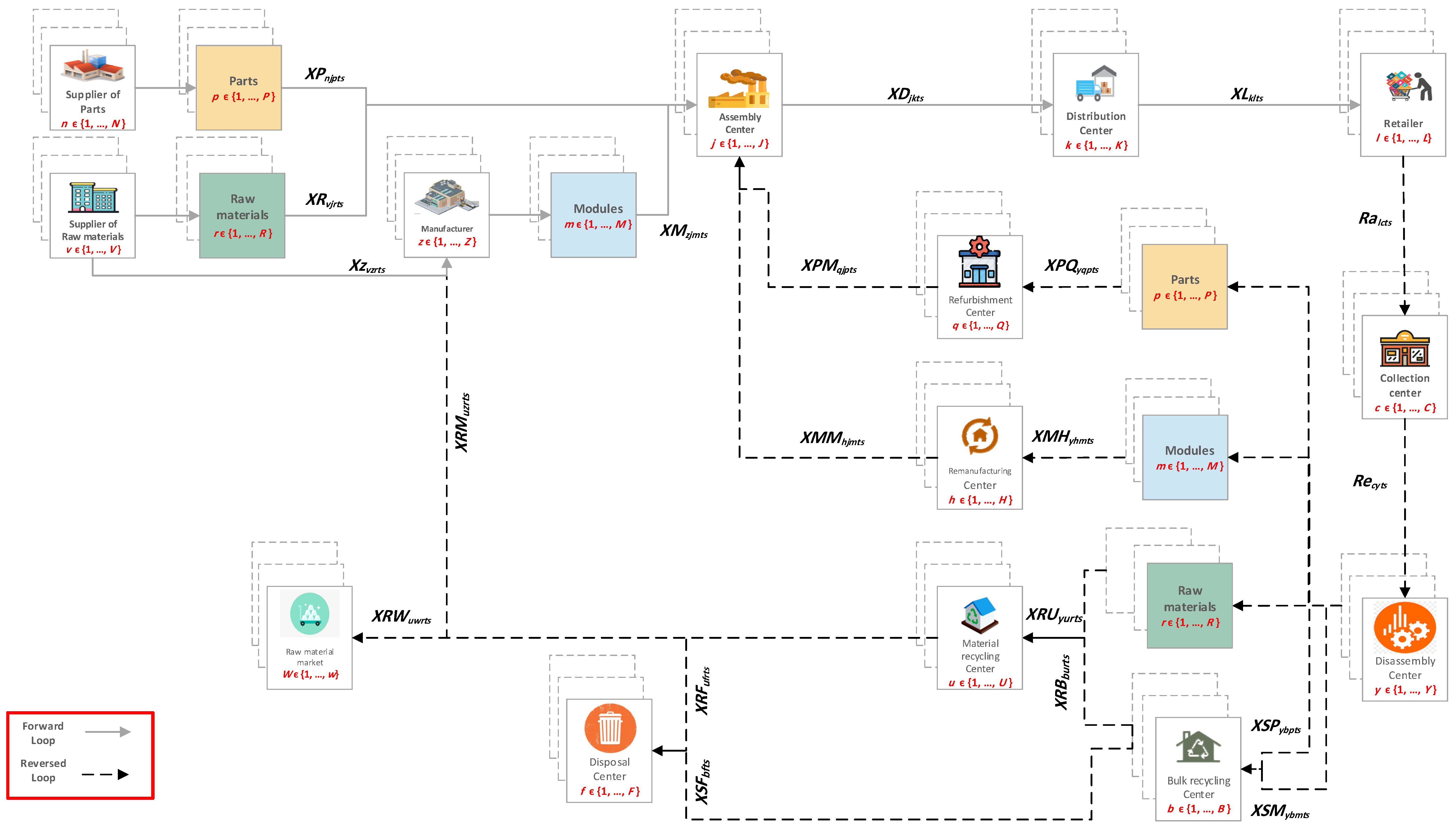
The CLSC network for a durable product shown in Figure 3 can be classified into the following two categories:

• Forward loop: The assembly center, j, procures the needed raw materials, r, and parts, p, from external suppliers; v and n, respectively. It gets the needed modules, m, from its manufacturer, z. Then assembly processes take place to produce the final product. After that, the products are distributed by a distribution center, k, to the final customer’s area, l, to be sold.
• Reverse loop: EOL products are collected from customer’s areas, l, through a collection center, c, and send to a disassembly center, y, where the product is broken down into its primary components: parts, modules, and raw material. Quality inspection is then done for each component to determine the suitable recovery option to be implemented, as follows:

  −

  Refurbishment: High-quality parts are shipped to a refurbishment center, q. This stage encourages materials to re-use activities (without further processing) such as cleaning, repairing, refurbishing, whole items, or spare parts.

  −

  Remanufacturing: High-quality modules are sent to the remanufacturing center, h. This stage aims to rebuild and recover the EOL product by disassembly, repair, and replace some of its components to return the product to a like-new condition.

  −

  Bulk recycling: Parts and modules with a low-quality level that cannot be refurbished and remanufactured but can be recycled for reuse as raw material are transferred to the bulk recycling center, b, wherein the precious raw materials are separated from scrap.

  −

  Recycling: The recyclable outputs of the bulk recycling center and the recyclable materials from the disassembly center are sent to the material recycling center, u. In this stage, recyclable materials are recovered for their value, and these materials are eventually sent to the manufacturer, z, or sold at an external raw material market, w.

  −

  Disposal: The non-recyclable outputs of both the bulk recycling center and material recycling center are shipped to disposal center, f.

3.2. Assumptions

The following assumptions are made:

−

New and recovered components will have the same quality grade (non-distinguishable).

−

All fixed and variable costs are known and fixed.

−

The selling price of the product and recycled material are fixed.

−

All retailers have the same demand level.

−

The raw material market has unlimited demand.

−

All facilities have limited and fixed capacities.

−

Once a facility is opened, it will be opened until the end of the planning horizon.

−

The life cycle of a durable product equals 5 years.

3.3. Mixed-Integer Linear Programming (MILP) Model Development

The necessary notations for indices, parameters, and decision variables and the mathematical formulation for designing a multi- echelon multi-period CLSC for durable products under uncertain demand, return rate, and return quality including the objective function and the related constraints are presented in the following subsections.

3.3.1. Notation

The necessary notations for indices, parameters, and decision variables of the proposed model are listed in

Table A1. Notation of indices.

Notation	Description
n ∈ {1, …, N}	Index of supplier of parts
z ∈ {1, …, Z}	Index of manufacturers
v ∈ {1, …, V}	Index of supplier of raw material
j ∈ {1, …, J}	Index of assembly centers
k ∈ {1, …, K}	Index of distribution centers
l ∈ {1, …, L}	Index of retailers
c ∈ {1, …, C}	Index of collection centers
y ∈ {1, …, Y}	Index of disassembly centers
f ∈ {1, …, F}	Index of disposal centers
t ∈ {1, …, T}	Index of time
q ∈ {1, …, Q}	Index of refurbishment centers
h ∈ {1, …, H}	Index of remanufacturing centers
b ∈ {1, …, B}	Index of bulk recycling centers
u ∈ {1, …, U}	Index of material recycling centers
p ∈ {1, …, P}	Index of parts needed to produce one unit of product
m ∈ {1, …, M}	Index of module needed to produce one unit of product
r ∈ {1, …, R}	Index of raw material needed to produce one unit of product
w ∈ {1, …, W}	Index of raw material markets
s ∈ {1, …, S}	Index of scenario
PSs	Probability of scenario s
βp	Number of part p that exists in one product
μm	Number of module m that exists in one product
ρr	Weight of raw material r (kg) that exists in one product
NPpr	Weight of raw material r (kg) that exists in one part p
NMmr	Weight of raw material r (kg) that exists in one module m
WPp	Weight of part p (kg)
WMm	Weight of module m (kg)
DEts	Demand for the product at time t under scenario s
αts (ALFA)	Percentage of returned parts and modules that can be refurbished and remanufactured at time t under scenario s
ðtS (FAI)	Return rate of EOL product at time t under scenario s

,

Table A2. Notation of parameters.

Notation	Description
Ralcts	Number of returned products shipped from retailer l to collection center c at time t under scenario s
Recyts	Number of returned products shipped from collection center c to disassembly center y at time t under scenario s
ηr	Recycling ratio of raw material r
CPNnp	Capacity of supplier n of part p
CPZzm	Capacity of manufacturer z of module m
CPVvr	Capacity of supplier v of raw material r
CPJj	Capacity of assembly center j
CPKk	Capacity of distribution center k
CPCc	Capacity of collection center c
CPYy	Capacity of disassembly center y
CPQq	Capacity of refurbishment center q
CPHh	Capacity of remanufacturing center h
CPUu	Capacity of material recycling center u
CPBb	Capacity of bulk recycling center b
CPFf	Capacity of disposal center f
TNnj	Shipping cost per unit of part from supplier n to assembly center j
TZzj	Shipping cost per unit of module from manufacturer z to assembly center j
TVvj	Shipping cost per kg of raw material from supplier v to assembly center j
TVZvz	Shipping cost per kg of raw material from supplier v to manufacturer z
TJjk	Shipping cost per unit of new product from assembly center j to distribution k
TLkl	Shipping cost per unit of new product from distribution k to retailer l
TRlc	Shipping cost per unit of used product from retailer l to collection center c
TYcy	Shipping cost per unit of used product from collection center c to disassembly center y
TQyq	Shipping cost per unit of part from disassembly center y to refurbishment center q
THyh	Shipping cost per unit of a module from disassembly center y to remanufacturing center h
TByb	Shipping cost per kg of residues from disassembly center y to bulk recycling center b
TUyu	Shipping cost per kg of raw material from disassembly center y to material recycling center u
TWuw	Shipping cost per kg of recycled material from material recycling center u to raw material market w
TMuz	Shipping cost per kg of recycled material from material recycling center u to manufacturer z
TDuf	Shipping cost per kg of raw material from material recycle center u to disposal center f
TEbf	Shipping cost per kg of waste from bulk recycle center b to disposal center f
TFbu	Shipping cost per kg of material from bulk recycle center b to material recycle center u
TGqj	Shipping cost per unit of refurbished part from refurbishment center q to manufacturing j
TKhj	Shipping cost of a unit of a remanufactured module from remanufacturing center h to assembly center j
ERr	Procurement cost per kg of raw material r
EMm	Manufacturing cost of a unit of module m
EPp	Procurement cost of a unit of part p
EN	Selling price of new product in case of no returns
ES	Selling price of new product in case of returns
EWr	Selling price per kg of raw material r in raw material market w
FCc	Fixed cost of opening collection center c
FYy	Fixed cost of opening disassembly center y
FFf	Fixed cost of opening disposal center f
FQq	Fixed cost of opening refurbishment center q
FHh	Fixed cost of opening remanufacturing center h
FBb	Fixed cost of opening bulk recycling center b
FUu	Fixed cost of opening material recycling center u
CJj	Assembly cost per unit of product at assembly center j
CKk	Distribution cost per unit of product at distribution center k
CCc	Processing cost per unit of product at collection center c
CYy	Disassembly cost per unit of product at disassembly center y
CQq	Refurbishment cost per unit of part at refurbishment center q
CHh	Remanufacturing cost per unit of a module at remanufacturing center h
CUu	Recycling cost per kg of raw material at material recycling center u
CBb	Processing cost per kg of residues at bulk recycling center b
CFf	Disposal cost per kg of waste at disposal center f

and

Table A3. Notation of decision variables.

Notation	Description
YCct	Binary variable equals 1 if collection center c is opened at time t, and 0 otherwise
YYyt	Binary variable equals 1 if disassembly center y is opened at time t, and 0 otherwise
YQqt	Binary variable equals 1 if refurbishment center q is opened at time t, and 0 otherwise
YHht	Binary variable equals 1 if remanufacturing center h is opened at time t, and 0 otherwise
YUut	Binary variable equals 1 if material recycling center u is opened at time t, and 0 otherwise
YBbt	Binary variable equals 1 if bulk recycling center b is opened at time t, and 0 otherwise
YFft	Binary variable equals 1 if disposal center f is open at time t, and 0 otherwise
XRvjrts	Quantity of purchased raw material r from supplier v for assembly center j at time t under scenario s
XZvzrt	Quantity of purchased raw material r from supplier v for manufacturer z at time t under scenario s
XMzjmts	Quantity of module m shipped from manufacturer z to assembly center j at time t under scenario s
XPnjpts	Quantity of purchased part p from supplier n for assembly center j at time t under scenario s
XDjkts	Quantity of new product shipped from assembly center j to distribution center k at time t under scenario s
XLklts	Quantity of new product shipped from distribution center k to retailer l at time t under scenario s
XPQyqpts	Number of refurbishable part p shipped from disassembly center y to refurbishment center q at time t under scenario s
XPMqjpts	Number of refurbished parts p shipped from refurbishment center q to assembly center j at time t under scenario s
XMHyhmts	Number of re-manufactural modules m shipped from disassembly center y to remanufacturing center h at time t under scenario s
XMMhjmts	Number of remanufactured modules m shipped from remanufacturing center h to assembly center j at time t under scenario s
XSPybpts	Number of non-recyclable parts p shipped from disassembly center y to bulk recycling center b at time t under scenario s
XSMybmts	Number of non-re-manufacturable modules m shipped from disassembly center y to bulk recycling center b at time t under scenario s
XRBburts	Quantity of recyclable material r shipped from bulk recycling center b to material recycling center u at time t under scenario s
XRUyurts	Quantity of raw material r shipped from disassembly center y to material recycling center u at time t under scenario s
XSFbfts	Quantity of non-recyclable material shipped from bulk recycling center b to disposal center f at time t under scenario s
XRFufrts	Quantity of non-recyclable material r shipped from material recycling center u to disposal center f at time t under scenario s
XRWuwrts	Quantity of recycled material r shipped from material recycling center u to raw material market w at time t under scenario s
XRMuzrts	Quantity of recycled material r shipped from material recycling center u to manufacturer z during t at time scenario s

in Appendix A.

3.3.2. Designing a CLSC

This study aims to design a multi- echelon and multi- period, t, CLSC for durable products under uncertain conditions. Each durable product consists of multi parts, p, modules, m, and various raw materials, r. The modular structure of a durable product is presented in Figure 4: β_p, μ_m, and ρ_r denote the number of parts, number of modules, and quantity of raw material that are required to produce one unit of a durable product. Moreover, each part, p, and each module, m, consist of a quantity of raw material, r, equal to NP_pr, NM_mr, respectively. In this study, a set of discrete scenarios, s, with probability PS_s, are used to illustrate the uncertainty in demand, DE_lts, return rate, ð_ts, and return quality, α_ts, for modules and parts. The objective function of the proposed MILP model is to optimize the profit of the CLSC, and it is formulated as stated in Equation (1).

Max. Profit = Total revenue − Cost of establishing facilities − Forward loop costs − Reversed loop costs

(1)

Let XL_kl(t−5)s represent the quantity of product that is shipped from distribution center, k, to the retailer, l, under scenario, s, with a discounted price, ES, in case of that the sold products at period t−5 are returned at time, t (since the life cycle of the durable product is 5 years), under scenario, s, at return rate, ð_ts. Then the first term of Equation (2) represents revenue that is obtained by selling a new product in the case of returns. The second term represents the revenue of selling a new product in the case of no returns; thus, XL_klts represents the quantity of product that is shipped from a distribution center, k, to a retailer, l at time, t, under scenario, s, and it is sold at normal price, EN. Further, the third term represents the revenue that is obtained by selling a quantity of recycled material, r, equals to XRW_uwrts, from a recycling material center, u, at raw material market, w, at time, t, under scenario, s, at price, EW_r. The total revenue is then calculated as stated in Equation (2).

$$\begin{array}{ll}Total revenue& ={\displaystyle {\displaystyle \sum }_{k=1}^K}{\displaystyle {\displaystyle \sum }_{l=1}^L}{\displaystyle {\displaystyle \sum }_{t=1}^T}{\displaystyle {\displaystyle \sum }_{s=1}^S}{PS}_S{ð}_{tS}{XL}_{kl\left(t-5\right)s}ES\\ & +{\displaystyle {\displaystyle \sum }_{k=1}^K}{\displaystyle {\displaystyle \sum }_{l=1}^L}{\displaystyle {\displaystyle \sum }_{t=1}^T}{\displaystyle {\displaystyle \sum }_{s=1}^S}{PS}_S\left({XL}_{klts}-{ ð}_{tS}{XL}_{kl\left(t-5\right)s}\right)EN \\ & +{\displaystyle {\displaystyle \sum }_{u=1}^U}{\displaystyle {\displaystyle \sum }_{w=1}^W}{\displaystyle {\displaystyle \sum }_{r=1}^R}{\displaystyle {\displaystyle \sum }_{t=1}^T}{\displaystyle {\displaystyle \sum }_{s=1}^S}{PS}_S{XRW}_{uwrts}{EW}_r \end{array}$$

(2)

Let us assume FC_c, FY_y, FQ_q, FH_h, FU_u, FB_b, and FF_f represent the fixed cost of establishing a collection center, c, disassembly center, y, refurbishment center, q, remanufacturing center, h, material recycling center, u, bulk recycling center, b, and disposal center, f, respectively. The values YC_ct, YY_yt, YQ_qt, YH_ht, YU_ut, YB_bt, and YF_ft are binary variables that determine whether facility c, y, q, h, u, b, f is opened at time t. These binary variables have a value of 1 if it decided to open the facility at time t, and 0 otherwise. The total fixed cost of establishing the facilities in the reversed loop is then calculated as stated in Equation (3).

$$\begin{array}{ll}\mathrm{Cost}\mathrm{of}\mathrm{establishing}\mathrm{facilitie}& \\ & ={\displaystyle {\displaystyle \sum }_{c=1}^C}{\displaystyle {\displaystyle \sum }_{t=1}^T}(Y{C}_{ct}- Y{C}_{c\left(t-1\right)})F{C}_c+{\displaystyle {\displaystyle \sum }_{y=1}^Y}{\displaystyle {\displaystyle \sum }_{t=1}^T}(Y{Y}_{yt}-Y{Y}_{y\left(t-1\right)})F{Y}_y\\ & +{\displaystyle {\displaystyle \sum }_{q=1}^Q}{\displaystyle {\displaystyle \sum }_{t=1}^T}(Y{Q}_{qt}-Y{Q}_{q\left(t-1\right)})F{Q}_q+{\displaystyle {\displaystyle \sum }_{h=1}^H}{\displaystyle {\displaystyle \sum }_{t=1}^T}(Y{H}_{ht}-Y{H}_{h\left(t-1\right)})F{H}_h\\ & +{\displaystyle {\displaystyle \sum }_{u=1}^U}{\displaystyle {\displaystyle \sum }_{t=1}^T}(Y{U}_{ut}-Y{U}_{u\left(t-1\right)})F{U}_u+{\displaystyle {\displaystyle \sum }_{b=1}^B}{\displaystyle {\displaystyle \sum }_{t=1}^T}(Y{B}_{bt}-Y{B}_{b\left(t-1\right)})F{B}_b\\ & +{\displaystyle {\displaystyle \sum }_{f=1}^F}{\displaystyle {\displaystyle \sum }_{t=1}^T}(Y{F}_{ft}-Y{F}_{f\left(t-1\right)})F{F}_{f }\end{array}$$

(3)

To calculate the total cost of the forward loop, let us assume XR_vjrts is the quantity of raw material, r, procured from a supplier, v, to assembly center, j, at time, t, under scenario, s, with purchasing cost ER_r, and shipping cost equal to TV_vj. This is stated in the first term of Equation (4). The second term represents shipping XZ_vzrts of the needed raw material, r, from supplier, v, to manufacturer, z, at time, t, under scenario, s, with purchasing cost ER_r, and shipping cost TVZ_vz. These materials are used to manufacture the required modules, m. The third term shows shipping XM_zjmts of the needed module, m, from manufacturer, z, to assembly center, j, at time, t, under scenario, s, with manufacturing cost, EM_m, and shipping cost, TZ_zj. The fourth term represents shipping XP_njpts of the needed part, p, from supplier, n, to assembly center, j, at time, t, under scenario, s, with purchasing cost, EP_p, and shipping cost, TN_nj. Let XD_jkts denote the quantity of products that are shipped from assembly center, j, to distribution center, k, at time, t, under scenario, s, and each product cost, CJj, as production cost and TJ_jk as shipping cost, and this is stated in the fifth term. The last term represents the quantity of product, XL_klts, that is shipped from distribution center, k, to retailer, l, at time, t, under scenario, s, and each product costs CK_k, and TL_kl, as processing and shipping cost, respectively. Accordingly, the total forward loop cost is calculated as stated in Equation (4).

$$\begin{array}{ll}\text{Forward loop costs}& \\ & ={\displaystyle {\displaystyle \sum }_{v=1}^V}{\displaystyle {\displaystyle \sum }_{j=1}^J}{\displaystyle {\displaystyle \sum }_{r=1}^R}{\displaystyle {\displaystyle \sum }_{t=1}^T}{\displaystyle {\displaystyle \sum }_{s=1}^S} P{S}_S\left(T{V}_{vj}+E{R}_r\right)X{R}_{vjrts}\\ & + {\displaystyle {\displaystyle \sum }_{v=1}^V}{\displaystyle {\displaystyle \sum }_{z=1}^Z}{\displaystyle {\displaystyle \sum }_{r=1}^R}{\displaystyle {\displaystyle \sum }_{t=1}^T}{\displaystyle {\displaystyle \sum }_{s=1}^S} P{S}_S\left(TV{Z}_{vz}+E{R}_r\right)X{Z}_{vzrts}\\ & +{\displaystyle {\displaystyle \sum }_{z=1}^Z}{\displaystyle {\displaystyle \sum }_{j=1}^J}{\displaystyle {\displaystyle \sum }_{m=1}^M}{\displaystyle {\displaystyle \sum }_{t=1}^T}{\displaystyle {\displaystyle \sum }_{s=1}^S} P{S}_S\left(T{Z}_{zj}+E{M}_m\right)X{M}_{zjmts}\\ & + {\displaystyle {\displaystyle \sum }_{n=1}^N}{\displaystyle {\displaystyle \sum }_{j=1}^J}{\displaystyle {\displaystyle \sum }_{p=1}^P}{\displaystyle {\displaystyle \sum }_{t=1}^T}{\displaystyle {\displaystyle \sum }_{s=1}^S} P{S}_S\left(T{N}_{nj}+E{P}_p\right)X{P}_{njpts} \\ & + {\displaystyle {\displaystyle \sum }_{j=1}^J}{\displaystyle {\displaystyle \sum }_{k=1}^K}{\displaystyle {\displaystyle \sum }_{t=1}^T}{\displaystyle {\displaystyle \sum }_{s=1}^S}P{S}_S\left(C{J}_j+T{J}_{jk}\right)X{D}_{jkts} \\ & + {\displaystyle {\displaystyle \sum }_{k=1}^K}{\displaystyle {\displaystyle \sum }_{l=1}^L}{\displaystyle {\displaystyle \sum }_{t=1}^T}{\displaystyle {\displaystyle \sum }_{s=1}^S}P{S}_S\left(C{K}_k+T{L}_{kl}\right)X{L}_{klts}\end{array}$$

(4)

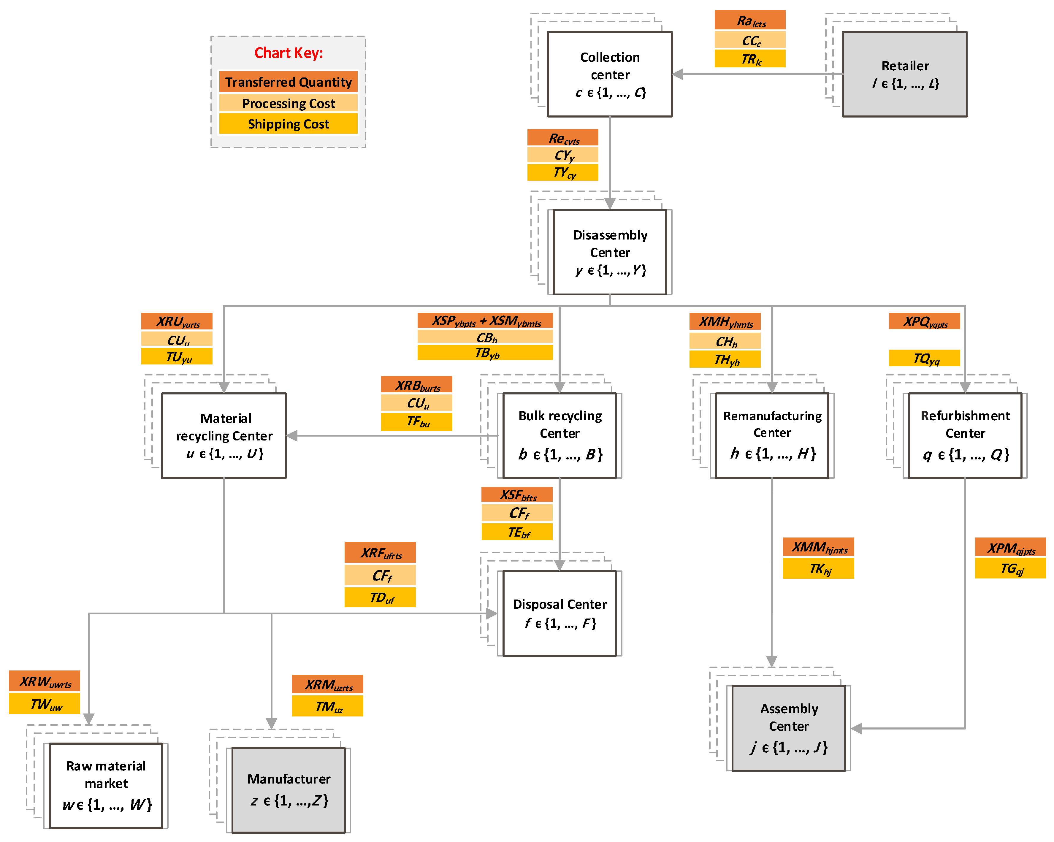
Figure 5 illustrates the quantity of components transferred between facilities in the reversed loop and the corresponding processing and shipping costs. The overall reversed loop cost is expressed mathematically as stated in Equation (5).

$$\begin{array}{ll}\mathrm{Reversed}\mathrm{loop}\mathrm{cost}& \\ & ={\displaystyle {\displaystyle \sum }_{l=1}^L}{\displaystyle {\displaystyle \sum }_{c=1}^C}{\displaystyle {\displaystyle \sum }_{t=1}^T}{\displaystyle {\displaystyle \sum }_{s=1}^S}P{S}_S\left(T{R}_{lc}+C{C}_c\right)R{a}_{lcts}\\ & +{\displaystyle {\displaystyle \sum }_{c=1}^C}{\displaystyle {\displaystyle \sum }_{y=1}^Y}{\displaystyle {\displaystyle \sum }_{t=1}^T}{\displaystyle {\displaystyle \sum }_{s=1}^S}P{S}_S\left(T{Y}_{cy}+C{Y}_y\right)R{e}_{cyts}\\ & +{\displaystyle {\displaystyle \sum }_{y=1}^Y}{\displaystyle {\displaystyle \sum }_{q=1}^Q}{\displaystyle {\displaystyle \sum }_{p=1}^P}{\displaystyle {\displaystyle \sum }_{t=1}^T}{\displaystyle {\displaystyle \sum }_{s=1}^S}P{S}_S\left(T{Q}_{yq}+C{Q}_q\right)XP{Q}_{yqpts}\\ & +{\displaystyle {\displaystyle \sum }_{q=1}^Q}{\displaystyle {\displaystyle \sum }_{j=1}^J}{\displaystyle {\displaystyle \sum }_{p=1}^P}{\displaystyle {\displaystyle \sum }_{t=1}^T}{\displaystyle {\displaystyle \sum }_{s=1}^S}P{S}_S\left(T{G}_{qj}\right)XP{M}_{qjpts}\\ & +{\displaystyle {\displaystyle \sum }_{y=1}^Y}{\displaystyle {\displaystyle \sum }_{h=1}^H}{\displaystyle {\displaystyle \sum }_{m=1}^M}{\displaystyle {\displaystyle \sum }_{t=1}^T}{\displaystyle {\displaystyle \sum }_{s=1}^S}P{S}_S\left(T{H}_{yh}+C{H}_h\right)XM{H}_{yhmts}\\ & +{\displaystyle {\displaystyle \sum }_{h=1}^H}{\displaystyle {\displaystyle \sum }_{j=1}^J}{\displaystyle {\displaystyle \sum }_{m=1}^M}{\displaystyle {\displaystyle \sum }_{t=1}^T}{\displaystyle {\displaystyle \sum }_{s=1}^S}P{S}_S\left(T{K}_{hj}\right)XM{M}_{hjmts}\\ & +{\displaystyle {\displaystyle \sum }_{y=1}^Y}{\displaystyle {\displaystyle \sum }_{b=1}^B}{\displaystyle {\displaystyle \sum }_{p=1}^P}{\displaystyle {\displaystyle \sum }_{t=1}^T}{\displaystyle {\displaystyle \sum }_{s=1}^S}P{S}_S\left(T{B}_{yb}+C{B}_b\right)XS{P}_{ybpts}\\ & +{\displaystyle {\displaystyle \sum }_{y=1}^Y}{\displaystyle {\displaystyle \sum }_{b=1}^B}{\displaystyle {\displaystyle \sum }_{m=1}^M}{\displaystyle {\displaystyle \sum }_{t=1}^T}{\displaystyle {\displaystyle \sum }_{s=1}^S}P{S}_S\left(T{B}_{yb}+C{B}_b\right)XS{M}_{ybmts}\\ & +{\displaystyle {\displaystyle \sum }_{b=1}^B}{\displaystyle {\displaystyle \sum }_{u=1}^U}{\displaystyle {\displaystyle \sum }_{r=1}^R}{\displaystyle {\displaystyle \sum }_{t=1}^T}{\displaystyle {\displaystyle \sum }_{s=1}^S}P{S}_S\left(T{F}_{bu}+C{U}_u\right)XR{B}_{burts}\\ & +{\displaystyle {\displaystyle \sum }_{b=1}^B}{\displaystyle {\displaystyle \sum }_{f=1}^F}{\displaystyle {\displaystyle \sum }_{t=1}^T}{\displaystyle {\displaystyle \sum }_{s=1}^S}P{S}_S\left(T{F}_{bf}+C{F}_f\right)XS{F}_{bfts}\\ & +{\displaystyle {\displaystyle \sum }_{y=1}^Y}{\displaystyle {\displaystyle \sum }_{u=1}^U}{\displaystyle {\displaystyle \sum }_{r=1}^R}{\displaystyle {\displaystyle \sum }_{t=1}^T}{\displaystyle {\displaystyle \sum }_{s=1}^S}P{S}_S\left(T{U}_{yu}+C{U}_u\right)XR{U}_{yurts}\\ & +{\displaystyle {\displaystyle \sum }_{u=1}^U}{\displaystyle {\displaystyle \sum }_{w=1}^W}{\displaystyle {\displaystyle \sum }_{r=1}^R}{\displaystyle {\displaystyle \sum }_{t=1}^T}{\displaystyle {\displaystyle \sum }_{s=1}^S}P{S}_S\left(T{W}_{uw}\right)XR{W}_{uwrts}\\ & +{\displaystyle {\displaystyle \sum }_{u=1}^U}{\displaystyle {\displaystyle \sum }_{z=1}^Z}{\displaystyle {\displaystyle \sum }_{r=1}^R}{\displaystyle {\displaystyle \sum }_{t=1}^T}{\displaystyle {\displaystyle \sum }_{s=1}^S}P{S}_S\left(T{M}_{uz}\right)XR{M}_{uzrts}\\ & +{\displaystyle {\displaystyle \sum }_{u=1}^U}{\displaystyle {\displaystyle \sum }_{f=1}^F}{\displaystyle {\displaystyle \sum }_{r=1}^R}{\displaystyle {\displaystyle \sum }_{t=1}^T}{\displaystyle {\displaystyle \sum }_{s=1}^S}P{S}_S\left(T{D}_{uf}+C{F}_f\right)XR{F}_{ufrts}\end{array}$$

(5)

This problem is subjected to various constraints regarding the capacities, fulfillment of demand, quantities needed to produce one unit of products, and other constraints. These constraints are presented as follows:

Let CPV_vr denote the maximum capacity of supplier, v, of raw-material, r. Equation (6) guarantees that capacity of supplier, v, will not be exceeded at any time and under all scenarios.

$${\displaystyle \sum }_{j=1}^{J}XR{}_{vjrts}+{\displaystyle \sum }_{z=1}^{Z}XZ{}_{vzrts}\le CPV{}_{vr} \forall v,r, t, s$$

(6)

Let CPZ_zm denote the maximum capacity of manufacturer, z, of module, m. Equation (7) guarantees that capacity of manufacturer, z, will not be exceeded at any time and under all scenarios.

$${\displaystyle \sum }_{j=1}^{J}XM{}_{zjmts}\le CPZ{}_{zm} \forall z,m, t, s$$

(7)

Let CPN_np denote the maximum capacity of supplier, n, of part, p. Equation (8) guarantees that capacity of supplier, n, will not be exceeded at any time and under all scenarios.

$${\displaystyle \sum }_{j=1}^{J}XP{}_{njpts}\le CPN{}_{np} \forall n,p, t, s$$

(8)

Let CPJ_j denote the maximum capacity of assembly center, j. Equation (9) guarantees that capacity of assembly center, j, will not be exceeded at any time and under all scenarios.

$${\displaystyle \sum }_{k=1}^{K}XD{}_{jkts}\le CPJ{}_j \forall j, t, s$$

(9)

Let us assume CPK_k denotes the maximum capacity of distribution center, k. Equation (10) guarantees that capacity of distribution center, k, will not be exceeded at any time and under all scenarios.

$${\displaystyle \sum }_{j=1}^{J}XD{}_{jkts}\le CPK{}_k \forall k, t, s$$

(10)

Let CPC_c denote the maximum capacity of collection center, c. Equation (11) guarantees that capacity of a collection center, c, will not be exceeded at any time and under all scenarios.

$${\displaystyle \sum }_{l=1}^{L}Ra{}_{lcts}\le CPC{}_C\times YC{}_{ct} \forall c,t, s$$

(11)

Let CPY_y denote the maximum capacity of disassembly center, y. Equation (12) guarantees that the capacity of a disassembly center, y, will not be exceeded at any time and under all scenarios.

$${\displaystyle \sum }_{c=1}^{C}Re{}_{cyts}\le CPY{}_y\times YY{}_{yt} \forall y,t, s$$

(12)

Let CPQ_q denote the maximum capacity of a refurbishment center, q. Equation (13) guarantees that the capacity of a refurbishment center, q, will not be exceeded at any time and under all scenarios.

$${\displaystyle \sum }_{y=1}^Y {\displaystyle \sum }_{p=1}^{P}XPQ{}_{yqpts}\le CPQ{}_q\times YQ{}_{qt} \forall q,t, s$$

(13)

Let CPH_h denote the maximum capacity of a remanufacturing center, h. Equation (14) guarantees that the capacity of a remanufacturing center, h, will not be exceeded at any time and under all scenarios.

$${\displaystyle \sum }_{y=1}^Y {\displaystyle \sum }_{m=1}^{M}XMH{}_{yhmts}\le CPH{}_h\times YH{}_{ht} \forall h,t, s$$

(14)

Let CPB_b denote the maximum capacity of a bulk recycling center, b. Equation (15) guarantees that the capacity of a bulk recycling center, b, will not be exceeded at any time and under all scenarios.

$${\displaystyle \sum }_{y=1}^Y {\displaystyle \sum }_{p=1}^P XSP{}_{ybpts}+{\displaystyle \sum }_{y=1}^Y {\displaystyle \sum }_{m=1}^{M}XSM{}_{ybmts}\le CPB{}_b\times YB{}_{bt} \forall b,t, s$$

(15)

Let CPU_u denote the maximum capacity of a material recycling center, u. Equation (16) guarantees that the capacity of a material recycling center, u, will not be exceeded at any time and under all scenarios.

$${\displaystyle \sum }_{y=1}^Y {\displaystyle \sum }_{r=1}^{R}XRU{}_{yurts}+{\displaystyle \sum }_{b=1}^B {\displaystyle \sum }_{r=1}^{R}XRB{}_{burts}\le CPU{}_u\times YU{}_{ut}\forall u,t, s$$

(16)

Let CPF_f denote the maximum capacity of a disposal center, f. Equation (17) guarantees that the capacity of a disposal center, f, will not be exceeded at any time and under all scenarios.

$${\displaystyle \sum }_{u=1}^U {\displaystyle \sum }_{r=1}^{R}XRF{}_{ufrts}+{\displaystyle \sum }_{b=1}^{B}XSF{}_{bfts}\le CPF{}_f\times YF{}_{f}t\forall f,t, s$$

(17)

Let DE_ts denote demand of retailer l, at time t, under scenarios s. Equation (18) guarantees that demand will be fully filled.

$${\displaystyle \sum }_{k=1}^{K}XL{}_{klts}=DE{}_{ts} \forall l,t, s$$

(18)

Let ð_ts denote the return rate of EOL product (which was sold at t − 5), at time t under scenario s. Equation (19) shows that the return quantity is a proportion of demand.

$${\displaystyle \sum }_{l=1}^L{\displaystyle \sum }_{c=1}^{C}Ra{}_{lcts}={\displaystyle \sum }_{k=1}^K {\displaystyle \sum }_{l=1}^{L}XL{}_{kl(t-5)s}\times ð{}_{\mathrm{ts}} \forall t, s$$

(19)

The input flow must equal the output flow for all facilities, as presented in Figure 3. This constraint is expressed mathematically as stated in Equations (20)–(25).

$${\displaystyle \sum }_{j=1}^{J}XD{}_{jkts}={\displaystyle \sum }_{l=1}^{L}XL{}_{klts}\forall k,t,s$$

(20)

$${\displaystyle \sum }_{l=1}^L{\displaystyle \sum }_{c=1}^{C}Ra{}_{lcts}={\displaystyle \sum }_{c=1}^C {\displaystyle \sum }_{y=1}^{Y}Re{}_{cyts} \forall t, s$$

(21)

$${\displaystyle \sum }_{y=1}^{Y}XPQ{}_{yqpts}={\displaystyle \sum }_{j=1}^{J}XPM{}_{qjpts}\forall q,p,t,s$$

(22)

$${\displaystyle \sum }_{y=1}^{Y}XMH{}_{yhmts}={\displaystyle \sum }_{j=1}^{J}XMM{}_{hjmts}\forall h,m,t,s$$

(23)

$${\displaystyle \sum }_{y=1}^{Y}XRU{}_{yurts}+{\displaystyle \sum }_{b=1}^{B}XRB{}_{burts}={\displaystyle \sum }_{w=1}^{W}XRW{}_{uwrts}+{\displaystyle \sum }_{z=1}^{Z}XRM{}_{uzrts}+{\displaystyle \sum }_{f=1}^{F}XRF{}_{ufrts}\forall u,r,t,s$$

(24)

$${\displaystyle \sum }_{y=1}^Y {\displaystyle \sum }_{p=1}^{P}WP{}_p\times XSP{}_{ybpts}+{\displaystyle \sum }_{y=1}^Y {\displaystyle \sum }_{m=1}^{M}WM{}_m\times XSM{}_{ybmts}={\displaystyle \sum }_{f=1}^{F}XSF{}_{bfts}+{\displaystyle \sum }_{u=1}^U {\displaystyle \sum }_{r=1}^{R}XRB{}_{burts}\forall b,t,s$$

(25)

Depending on the modular structure of a durable product, the assembly center, j, requires a quantity of part, p, equal to β_p. It gets this quantity from part supplier, n, and from a refurbishment center, q, to produce one unit of product. This quantity can be calculated as stated in Equation (26).

$${\displaystyle \sum }_{n=1}^{N}X{P}_{njpts }+{\displaystyle \sum }_{q=1}^{Q}XP{M}_{qjpts }={\displaystyle \sum }_{k=1}^K\left({\beta }_P\right)\times X{D}_{jkts }\forall j,p,t,s$$

(26)

Assembly center, j, requires a quantity of module, m, equal to μ_m. It gets this quantity from manufacturer, z, and from a remanufacturing center, h, to produce one product. This quantity can be calculated as stated in Equation (27).

$${\displaystyle \sum }_{z=1}^{Z}X{M}_{zjmts }+{\displaystyle \sum }_{h=1}^{H}XM{M}_{hjmts }={\displaystyle \sum }_{k=1}^K\left({\mu }_m\right)\times X{D}_{jkts }\forall j,m,t,s$$

(27)

Assembly center, j, requires a quantity of raw material, r, equals to ρ_r. It gets this quantity from raw material supplier, v, to produce one product. This quantity can be calculated as stated in Equation (28).

$${\displaystyle \sum }_{v=1}^{V}X{R}_{vjrts }={\displaystyle \sum }_{k=1}^K\left({\rho }_r\right)\times X{D}_{jkts }\forall j,r,t,s$$

(28)

To produce one unit of module, m, in manufacturer, z, at time, t, under scenario, s, a quantity of raw material, r, equals to NM_mr is needed. These quantities are shipped to manufacturer, z, from supplier, v, and material recycling center, u, and can be mathematically presented in Equation (29).

$${\displaystyle \sum }_{v=1}^{V}XZ{}_{vzrts}+{\displaystyle \sum }_{u=1}^{U}XRM{}_{uzrts}={\displaystyle \sum }_{j=1}^J {\displaystyle \sum }_{m=1}^{M}NM{}_{mr}\times XM{}_{zjmts} \forall z,r,t,s$$

(29)

The returned parts lie in different quality levels and depending on the quality level, the recovery option is chosen. Let α_ts denote the percentage of each returned part able to be refurbished at time, t, under scenario, s. The number of parts is shipped from disassembly center, y, to refurbished center, q, at time, t, can be mathematically represented as in Equation (30).

$${\displaystyle \sum }_{y=1}^Y {\displaystyle \sum }_{q=1}^{Q}XP{Q}_{yqpts }={\displaystyle \sum }_{c=1}^C {\displaystyle \sum }_{y=1}^Y\left({\beta }_p\right)\times \left({\alpha }_{ts }\right)\times R{e}_{cyts }\forall p,t,s$$

(30)

Tthe non-refurbishable parts are shipped from disassembly center, y, to bulk recycling center, b, at time, t, under scenario, s, as presented in Equation (31).

$${\displaystyle \sum }_{y=1}^Y {\displaystyle \sum }_{b=1}^{B}XS{P}_{ybpts }={\displaystyle \sum }_{c=1}^C {\displaystyle \sum }_{y=1}^Y\left({\beta }_p\right)\times \left(1-{\alpha }_{ts }\right)\times R{e}_{cyts }\forall p,t,s$$

(31)

Let α_ts denote the percentage of each returned module able to be remanufactured under scenario, s, then the number of modules shipped from disassembly center, y, to remanufacturing center, h, at time, t, can be mathematically represented as in Equation (32).

$${\displaystyle \sum }_{y=1}^Y{\displaystyle \sum }_{h=1}^{H}XM{H}_{yhmts }={\displaystyle \sum }_{c=1}^C{\displaystyle \sum }_{y=1}^Y\left({\mu }_m\right)\times \left({\alpha }_{ts }\right)\times R{e}_{cyts } \forall m,t,s$$

(32)

The non-remanufacturable modules are shipped from disassembly center, y, to bulk recycling center, b, at time, t, under scenario, s, as presented in Equation (33).

$${\displaystyle \sum }_{y=1}^Y{\displaystyle \sum }_{b=1}^{B}XS{M}_{ybmts }={\displaystyle \sum }_{c=1}^C{\displaystyle \sum }_{y=1}^Y\left( {\mu }_m\right)\times \left(1-{\alpha }_{ts }{}_{ }\right)\times R{e}_{cyts } \forall m,t,s$$

(33)

The quantity of raw material, r, shipped from disassembly center, y, to material recycling center, u, at time, t, under scenario, s, is mathematically presented in Equation (34).

$${\displaystyle \sum }_{y=1}^Y{\displaystyle \sum }_{u=1}^{U}XR{U}_{yurts }={\displaystyle \sum }_{c=1}^C{\displaystyle \sum }_{y=1}^Y\left({\rho }_r\right)\times R{e}_{cyts } \forall r,t,s$$

(34)

Let η_r denote the recycling ratio of raw material r. The non-recyclable material shipped from material recycling center, u, to disposal center, f, at time, t, under scenario, s, is mathematically presented as stated in Equation (35).

$${\displaystyle \sum }_{u=1}^U{\displaystyle \sum }_{f=1}^{F}XRF{}_{ufrts}={\displaystyle \sum }_{y=1}^Y{\displaystyle \sum }_{u=1}^U\left(1-{\eta }_r\right)\times XRU{}_{yurts} \forall r,t,s$$

(35)

Based on the quantity of raw material r, existing in one unit of part, p, and module, m, the quantity of raw material r shipped from bulk recycling center, b, to material recycling center u, at time, t, under scenario, s, is mathematically expressed in Equation (36).

$$\begin{array}{ll}{\displaystyle {\displaystyle \sum }_{b=1}^B}{\displaystyle {\displaystyle \sum }_{u=1}^U}XRB{}_{burts}& ={\displaystyle {\displaystyle \sum }_{y=1}^Y}{\displaystyle {\displaystyle \sum }_{b=1}^B}{\displaystyle {\displaystyle \sum }_{p=1}^P} \left({\eta }_r\right)\times \left(NP{}_{pr}\right)\times XS{P}_{ybpts }\\ & +{\displaystyle {\displaystyle \sum }_{y=1}^Y}{\displaystyle {\displaystyle \sum }_{b=1}^B}{\displaystyle {\displaystyle \sum }_{m=1}^M}\left({\eta }_r\right)\times \left(NM{}_{mr}\right)\times XS{M}_{ybmts }\forall r,t,s\end{array}$$

(36)

It is assumed that once a collection center, c, is opened, it will be open until the end of the planning horizon; this is guaranteed by Equation (37).

$$YC{}_{ct} \le YC{}_{ct+1} \forall c, t=T-1 .$$

(37)

It is assumed that once a disassembly center, y, is opened, it will be open until the end of the planning horizon; this is guaranteed by Equation (38).

$$YY{}_{yt} \le YY{}_{yt+1} \forall y, t=T-1$$

(38)

It is assumed that once a refurbishing center, q, is opened, it will be open until the end of the planning horizon; this is guaranteed by Equation (39).

$$YQ{}_{qt} \le YQ{}_{qt+1} \forall q, t=T-1$$

(39)

It is assumed that once a remanufacturing center, h, is opened, it will be open until the end of the planning horizon; this is guaranteed by Equation (40).

$$YH{}_{ht} \le YH{}_{ht+1} \forall h, t=T-1$$

(40)

It is assumed that once a material recycling center, u, is opened, it will be open until the end of the planning horizon; this is guaranteed by Equation (41).

$$YU{}_{ut} \le YU{}_{ut+1} \forall u, t=T-1$$

(41)

It is assumed that once a bulk recycling center, b, is opened, it will be open until the end of the planning horizon; this is guaranteed by Equation (42).

$$YB{}_{bt} \le YB{}_{bt+1} \forall b, t=T-1$$

(42)

It is assumed that once a disposal center, f, is opened, it will be open until the end of the planning horizon; this is guaranteed by Equation (43).

$$YF{}_{ft} \le YF{}_{ft+1} \forall f, t=T-1$$

(43)

As the decision variables of opening the facilities in the reversed loop is a binary variable having only two possible values of 0 or 1, then this binary constraint is presented in Equation (44).

YC_ct, YY_yt, YQ_qt, YH_ht, YU_ut, YB_bt, and YF_ft ∈ {0, 1}

(44)

Non-negativity is guaranteed by constraint in Equation (45):

XM_zjmts, XP_njpts, XD_jkts, XL_klts, Ra_lcts, Re_cyts, XPQ_yqpts, XPM_qjpts, XMH_yhmts,
XMM_hjmts, XSM_ybmts, XSP_ybpts, XR_vjrts, XZ_vzrts, XRB_burts, XRU_yurts, XSF_bfts, XRF_ufts,
XRW_uwrts, and XRM_uzrts ≥ 0

(45)

4. Model Application and Results

4.1. Model Application

To test the efficiency of the proposed MILP formulation for a real-life application, a case study of an air conditioner (AC) manufacturing company in Jordan is considered. This company produces several types of products, and it is working on producing a new type of mini-split unit (AC) that will be available at markets during the end of this year. This type of mini-split unit is used in this study. This supply chain consists of 1 supplier of parts (N = 1), 2 suppliers of raw material (V = 2), 3 manufacturers (Z = 3), 3 assembly centers (J = 3), 1 distribution center (K = 1), and 4 retailers (L = 4). The related parameters for this supply chain are presented in

Table 2. Forward loop parameters.

Assembly Center	j1	j2	j3
Capacity (unit/year)	CPJ1 = 14,000	CPJ2 = 12,500	CPJ3 = 13,800
Assembly and overhead cost (USD/product)	CJ1 = 6.43	CJ2 = 6.43	CJ3 = 6.43
Manufacturer	z1	z2	z3
Capacity (unit/year)	CPZ11 = 14,000	CPZ21 = 12,500	CPZ31 = 13,800
	CPZ12 = 14,000	CPZ22 = 12,500	CPZ32 = 13,800
	CPZ13 = 14,000	CPZ23 = 12,500	CPZ33 = 13,800
Processing cost (USD/unit)	EM1 = 5.35	EM1 = 5.35	EM1 = 5.35
	EM2 = 5.35	EM2 = 5.35	EM2 = 5.35
	EM1 = 2.7	EM1 = 2.7	EM1 = 2.7
Distribution center	k1
Capacity (unit/year)	CPK = 16,500
Processing cost (USD/product)	CK1 = 0.18
Suppliers	n1	v1	v2
Capacity (unit/year)	CPN11 = 80,000	CPV11 = 300,000	CPV21 = 350,000
	CPN12 = 80,000	CPZ12 = 200,000	CPZ22 = 300,000
	CPN13 = 80,000	CPZ13 = 200,000	CPZ23 = 200,000
	CPN14 = 80,000	CPN14 = 200,000	CPN24 = 200,000
		CPZ15 = 200,000	CPZ25 = 200,000

.

This manufacturing company produces condensers, evaporators, and sheet metal, whereas the other components are purchased from an external supplier. The components are then assembled in the assembly centers to produce the final AC unit. Accordingly, to address this case study well, it will be assumed that modules represent the components that are being manufactured at the manufacturers. Accordingly, based on the reverse BOM, this type of AC unit consists of 4 parts (P = 4), 3 modules (M = 3), and 5 types of raw material (R = 5). The weight of each component, the quantity of each component per AC unit, the BOM for each component, and the purchasing costs are presented in

Table 3. Modular structure of AC unit.

Component Name	Component Index	Weight (kg)	Quantity/AC Unit	BOM	Material Quantity	Price (USD)
Blower	p1	WP1 = 4.3	β1= 2	Plastic	NP14 = 1.3	36.15
				Copper	NP11 = 1.2
				Steel	NP12 = 1.8
Filters	p2	WP2 = 0.2	β2 = 2	Plastic	NP24 = 0.2	3.55
Compressor	p3	WP3 = 18.2	β3 = 1	Copper	NP31 = 6.6	75.2
				Steel	NP32 = 11.6
Frame for internal unit	p4	WP4 = 2.3	β4 = 1	Plastic	NP44 = 2.3	14.20
Evaporator	m1	WM1 = 18.2	μ1 = 1	Copper	NM1 = 3.8	____
				Aluminum	NM13 = 3.8
Condenser	m2	WM2 = 8.2	μ2 = 1	Copper	NM21 = 4.1	____
				Aluminum	NM23 = 4.1
Frame for external unit	m3	WM3 = 3.5	μ3 = 1	Steel	NM32 = 3.5	____
Copper pipes	r1	_____	ρ1 = 2	Copper	____	8.7
Other	r5	_____	ρ5 = 1	Non-recyclable material	____	2.8

.

The purchasing cost and selling price per 1 kg of raw material, r, and the recycling ratio of raw material, r, are presented in

Table 4. The selling price of raw material.

Raw Material	Index	Purchasing Cost USD/kg	Sale Price at W Market USD/kg	Recycling Ratio
Copper	r1	8.7	6	η1 = 1
Steel	r2	1.2	1	η2 = 0.65
Aluminum	r3	2.5	2	η3 = 0.95
Plastic	r4	2	1.5	η4 = 0.80
Non-recyclable materials	r5	2.8	Not-applicable	η5 = 0

.

The reversed loop does not exist yet in this AC manufacturing company; hence the estimation costs and other reversed loop parameters are taken from the literature. Most of the data are extracted and/or inspired from the case study of Indian based manufacturing unit of a Saudi Arabian industrial air conditioner manufacturing organization that was presented in [29]. The parameters related to reversed facilities are presented in

Table 5. Reversed loop parameters.

Collection Centers	c1	c2	c3
Fixed cost of establishing the facility (USD)	100,000	120,000	110,000
Capacity (unit/year)	CPC1 = 6000	CPC2 = 8000	CPC3 = 7000
Processing cost (USD/product)	CC1 = 0.15	CC2 = 0.15	CC3 = 0.15
Disassembly Centers	y1	y2
Fixed cost of establishing the facility (USD)	120,000	110,000
Capacity (unit/year)	CPY1 = 8000	CPY2 = 7000
Processing cost (USD/product)	CY1 = 6.3	CY2 = 6.3
Remanufacturing Centers	h1	h2
Fixed cost of establishing the facility (USD)	300,000	250,000
Capacity (unit/year)	CPH1 = 50,000	CPH2 = 60,000
Processing cost (USD/unit)	CH1 = 3.6	CH2 = 3.6
Material Recycling Centers	u1	u2
Fixed cost of establishing the facility (USD)	190,000	170,000
Capacity (kg/year)	CPU1 = 55,000	CPU2 = 40,000
Processing cost (USD/kg)	CU1 = 1.4	CU2 = 1.4
Bulk recycling Centers	b1	b2
Fixed cost of establishing the facility (USD/Kg)	170,000	150,000
Capacity (kg/year)	CPB1 = 45,000	CPB2 = 40,000
Processing cost (USD/unit)	CB1 = 1.3	CB2 = 1.3
Refurbishment Centers	q1	q2
Fixed cost of establishing the facility (USD)	250,000	200,000
Capacity (unit/year)	CPQ1 = 40,000	CPQ2 = 35,000
Processing cost (USD/part)	CQ1 = 2.1	CQ2 = 2.1
Disposal Centers	f1	f2
Fixed cost of establishing the facility (USD)	80,000	85,000
Capacity (kg/year)	CPF1 = 20,000	CPF2 = 25,000
Processing cost (USD/kg)	CF1 = 0.4	CF2 = 0.4

.

The selling price of this type of AC unit at the user market is 349 USD, which includes transportation and installation costs. To encourage customers to return their EOL products, a discount policy of (20%) on the selling price is proposed in the case of returned EOL products; thus, the selling price of a new AC is 280 USD in the case of returns. The potential location of the reversed loop facilities is presented in Figure A1 in Appendix B. The maximum capacity of the trucks that are used to transfer different components between the facilities is 6 tons, and fuel consumption is 23.7 L/100 km. The price of the fuel is 0.783 USD/L, and the average weight of an AC unit is 65 kg, the average weight for modules is 10 kg, and the average weight for parts is 6 kg. Accordingly, the average transportation cost between two facilities per unit is presented in

Table A4. Transportation costs in the CLSC (USD/unit).

	j1	j2	j3			y1	y2
k1	0.1	0.1	0.18		u1	0.05	0.15
	k1				u2	0.15	0.04
l1	0.01					u1	u2
l2	0.03				z1	0.03	0.15
l3	0.21				z2	0.03	0.15
l4	0.66				z3	0.15	0.04
	l1	l2	l3	l4		u1	u2
c1	0.01	0.03	0.22	0.66	f1	0.03	0.15
c2	0.23	0.22	0.02	0.86	f2	0.15	0.04
c3	0.66	0.66	0.86	0.01		b1	b2
	c1	c2	c3		f1	0.07	0.15
y1	0.1	0.24	0.67		f2	0.15	0.05
y2	0.18	0.09	0.78			b1	b2
	y1	y2			u1	0.05	0.15
q1	0.01	0.15			u2	0.15	0.03
q2	0.15	0.02				q1	q2
	y1	y2			j1	0.04	0.15
h1	0.04	0.15			j2	0.04	0.15
h2	0.15	0.05			j3	0.15	0.05
	y1	y2				h1	h2
b1	0.04	0.15			j1	0.05	0.15
b2	0.15	0.03			j2	0.05	0.15
					j3	0.15	0.06

in Appendix A.

Further, the demand, return rate of EOL products, and quality of these returns are assumed to be stochastic (uncertain) variables. These uncertain declarations are presented in

Table 6. Uncertainty in the proposed model.

Random Variable	Distribution	Mean	Sigma
Demand (unit/year)	Normal distribution	1300	65
Random Variable	Mode	Value	Probability
Return rate	Optimistic	0.75	0.45
	Pessimistic	0.45	0.55
Return quality	Good	0.80	0.45
	Poor	0.65	0.55

. LINGO 18.0 optimization package was used to code and solve the proposed MILP model. The model developed according to the above data for 7 periods was computed with LINGO 18.0 on a personal computer with Intel Core i5-9300H 2.4 GHz (8 CPUs) processor and 32 GB memory under the Windows 10 operating system. Because normal distribution gives infinite possible outcomes for the random variable assigned to it, the Monte Carlo sampling technique is used to generate the scenarios regarding the uncertain variables. The sample size is set to 2; thus, 2 samples are generated at each stage (period). This study consists of 7 stages, hence the total number of scenarios for all stages 1 to 7 equals to 2⁷ =128 scenarios. A multi-stage stochastic approach was used to solve this problem. In stage zero, a decision of establishing the facilities in the reversed loop is taken, whereas in the following stages the quantities of purchasing of raw material (XZ and XR), purchasing of parts (XP), manufacturing (XM), assembling (XD), distributing (XL), refurbishing (XPQ), refurbished parts are shipped to assembly center (XPM), remanufacturing (XMH), remanufactured modules are shipped to assembly center (XMM), recycling (XRU and XRB), bulk recycling (XSP and XSM), recycled material are shipped to the manufacturer (XRM), disposing (XSF and XRF), and selling raw material at the material market (XRW) are determined.

4.2. Computational Results

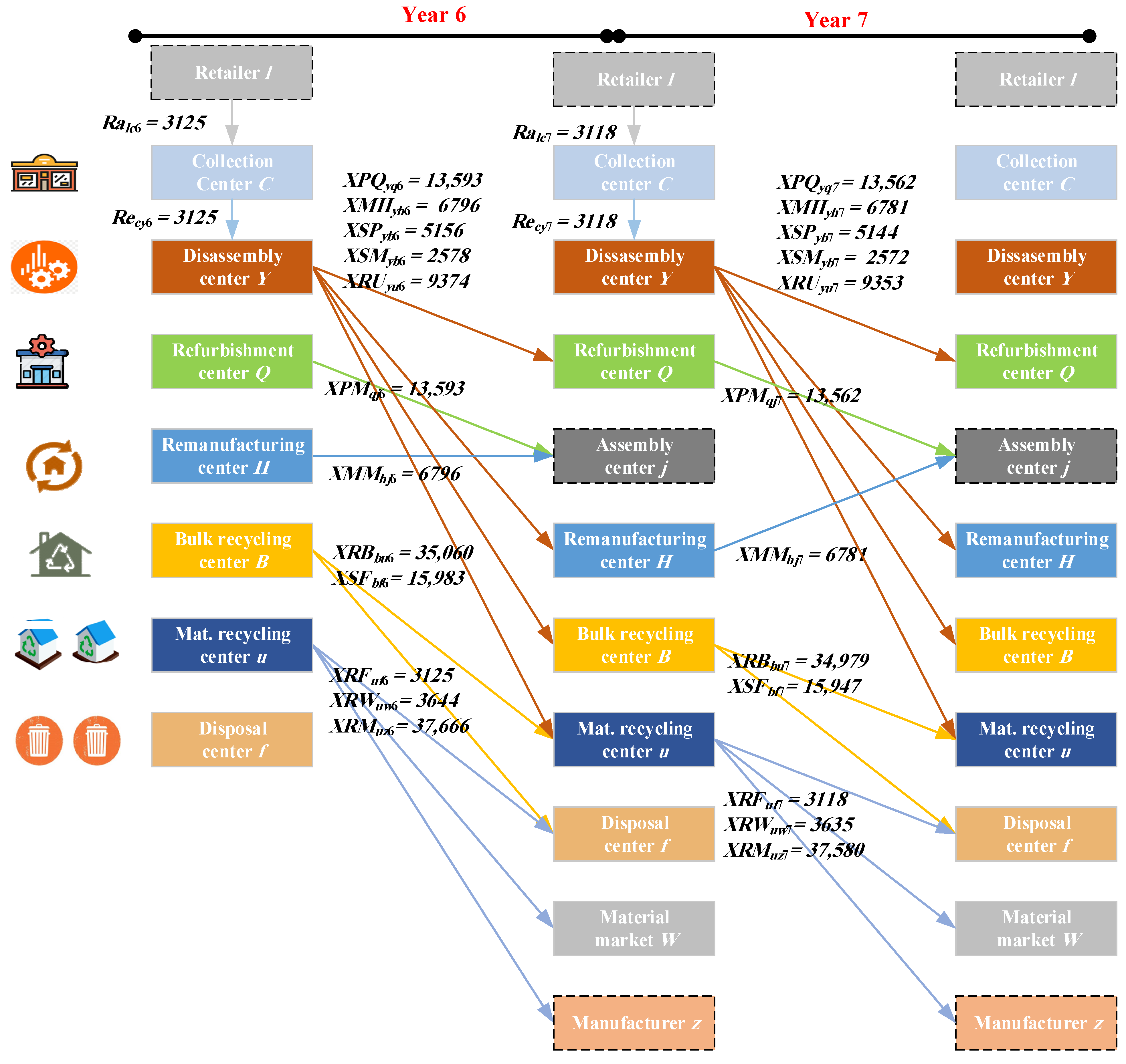
The elapsed time for solving this problem was 140.37 s, and the total number of iterations that were used to obtain the global optimal solution was 469,021. The global optimal profit is 1,239,664 USD. The decision variables of stage zero are presented in

Table 7. Optimal values of decision variables at stage zero.

Decision Variable	Value	Decision Variable	Value	Decision Variable	Value
YC (1, t6)	1	YB (2, t6)	1	YH (1, t7)	1
YY (2, t6)	1	YF (1, t6)	1	YU (1, t7)	1
YQ (2, t6)	1	YF (2, t6)	1	YU (2, t7)	1
YH (1, t6)	1	YC (1, t7)	1	YB (2, t7)	1
YU (1, t6)	1	YY (2, t7)	1	YF (1, t7)	1
YU (2, t6)	1	YQ (2, t7)	1	YF (2, t7)	1

. Accordingly, the first collection center (c₁), the second disassembly center (y₂), the second refurbishment center (q₂), the first remanufacturing center (h₁), the first and the second material recycling centers (u₁, u₂), the second bulk recycling center (b₂), and both the first and second disposal centers (f₁, f₂) were decided to be opened at period 6 and they still are open until the end of planning horizon (t₇). Hence, the CLSC design will exist at periods 6 and 7. Some of scenarios that present the possible outcomes of the random variables of the proposed problem and their cross-bonding profit are presented in

Table 8. Set of scenarios.

Scenario #	Profit USD	Scenario #	Profit USD	Scenario #	Profit USD
1	1,243,831	2	1,396,961	3	1,084,144
4	1,237,274	5	1,258,475	6	1,411,605
. . .	. . .	. . .	. . .	. . .	. . .
91	1,095,301	92	1,248,431	93	1,270,115
. . .	. . .	. . .	. . .	. . .	. . .
123	1,067,832	124	1,220,259	125	1,242,646
126	1,395,073	127	1,082,476	128	1,234,904

.

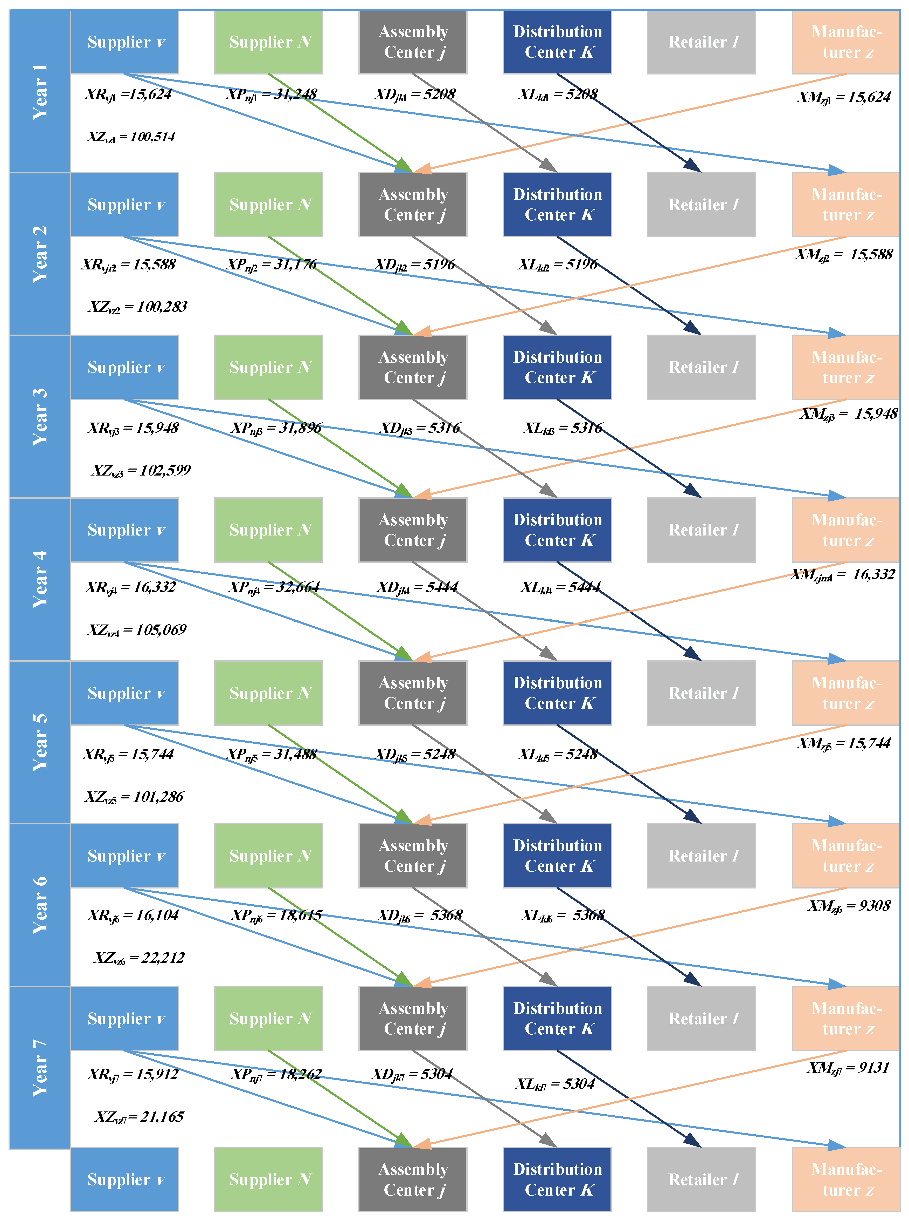
To present the optimal quantities of purchasing, production, distributing, selling, recycling, remanufacturing, refurbishing, and disposing, the mean values of the random variables in all 128 scenarios are taken from the random variable distribution report as presented in Figure 6, then these values with the optimal values of the decision variables of stage zero are used to test the performance of the CLSC as a deterministic model. After running the model for 7 periods, the obtained optimal quantities for both forward and reversed loop are plotted in Figure 7 and Figure 8, respectively.

Converting the FSC into CLSC has various types of expenses, savings, and revenues. To present the quantities of savings and expenses of the CLSC, the values from the random distribution report are used to test the performance of both FSC and CLSC. In FSC, demand means are taken from the report and the return rate is set to 0. The obtained results in regard to the expenses and revenues for both cases at periods 6 and 7 are listed in

Table 9. Comparison between FSC and CLSC.

Metrix	Period 6		Period 7		Average Δ	Average Δ in USD
	FSC	CLSC	FSC	CLSC
Annual purchasing cost	1,583,989	751,880	156,5104	734,912	−0.52	831,150
Annual transportation cost	2000	8449	1976	8441	+3.25	6457
Annual reversed processing cost	___	153,073	___	152,720	___
Annual revenue from selling raw material	___	5465	___	5453	___

. Accordingly, CLSC for the proposed case study reduced the purchasing cost by 52%; thus, the annual saving in purchasing cost is about 831,150 USD. However, CLSC increases the transportation cost by 3.25 times compared to the FSC case. In other words, the annual transportation cost related to the reversed loop is 6457 USD. CLSC in the proposed case study costs 152,897 USD as an annual processing cost in the reversed loop facilities. Moreover, the annual revenue of selling raw materials at the external material market is about 5459 USD.

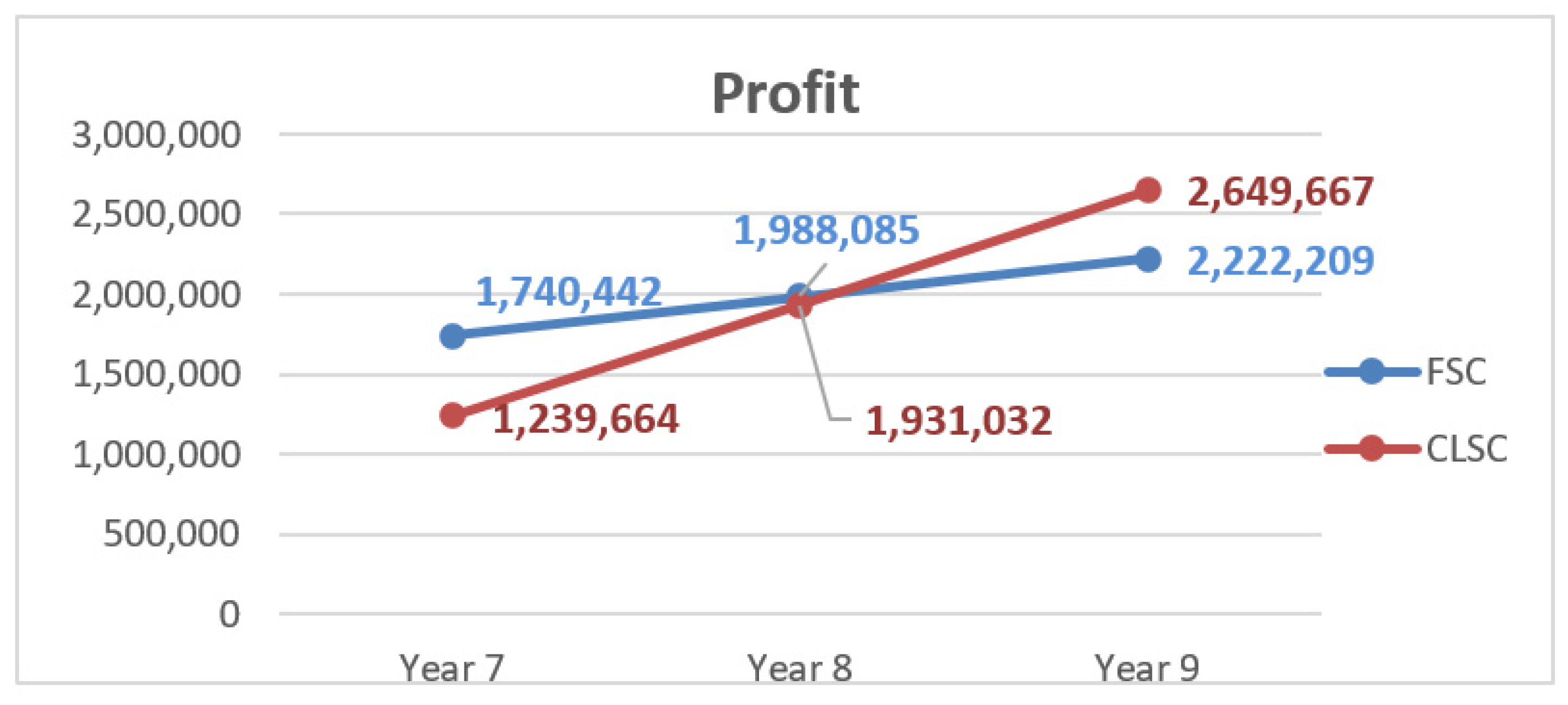
In order to examine the performance of the CLSC in the long run while the uncertainty in demand, return rate, and return quality are presented, the stochastic model was run for 9 periods for both FSC and CLSC cases. In the FSC case, the return rate is set to 0.

Table 10. Obtained profit in FSC and CLSC.

Class	Year 7	Year 8	Year 9
FSC	1,740,442	1,988,085	2,222,209
CLSC	1,239,664	1,931,032	2,649,667

presents the obtained profit in each case.

Recall that the CLSC existed at period 6 and according to Table 10, the profit in the FSC case is greater than in the CLSC case for the first three years of the existence of the CLSC (periods 6–8). However, in year 9 CLSC has a higher profit than the FSC. In other words, the break-even point occurs after 3 years of establishing the CLSC as presented in Figure 9, and this is expected since opening a facility is a strategic decision that needs many years to reverse back the investment expense. Consequently, in year 4 of establishing the CLSC, it is expected that the profit of the current case study will increase by 1.92%.

4.3. Sensitivity Analysis

To analyze the effect of decreasing the values of both demand and return rate on the CLSC performance, a sensitivity analysis was conducted as follows.

4.3.1. Changing Demand Level

The demand level was increased and decreased by 10% and 20%, and the obtained result (on an annual basis) for each case is presented under scenario 92 for periods 6 and 7 in

Table 11. Sensitivity analysis on demand for period 6.

Scenario 92	Period 6
	−20%	−10%	Initial	+10%	+20%	∆
Optimal profit (USD)	795,563	977,922	1,239,664	1,501,097	1,762,911
Scenario profit (USD)	802,586	985,918	1,248,431	1,510,667	1,773,014
Fixed cost (USD)	1,305,000	1,385,000	1,385,000	1,385,000	1,385,000
Forward transportation cost (USD)	1666	1873	2080	2289	2497
Reversed transportation cost (USD)	3350	3768	4186	4604	5022
Purchasing cost (USD)	702,187	789,494	876,800	965,286	1,052,593
Quantity sold at discounted price (unit)	1904	2142	2380	2,617	2855
Revenue from selling raw material at material market (USD)	2422	2725	3027	3329	3631
Quantity of returned EOL (unit)	1904	2142	2380	2617	2855
Total forward cost (USD)	729,579	820,296	911,013	1,002,937	1,093,654
Reversed processing cost (USD)	85,740	96,437	107,134	117,832	128,529

and

Table 12. Sensitivity analysis on demand for period 7.

Scenario 92	Period 7
	−20%	−10%	Initial	+10%	+20%	∆
Optimal profit (USD)	795,563	977,922	1,239,664	1,501,097	1,762,911
Scenario profit (USD)	802,586	985,918	1,248,431	1,510,667	1,773,014
Fixed cost (USD)	1,305,000	1,385,000	1,385,000	1,385,000	1,385,000
Forward transportation cost (USD)	1788	2012	2235	2458	2682
Reversed transportation cost (USD)	7579	8684	10,233	11,937	13,653
Purchasing cost (USD)	528,545	594,398	660,252	726,520	792,373
Quantity sold at discounted price (unit)	3186	3585	3984	4380	4779
Revenue from selling raw material at material market (USD)	55,638	62,683	69,729	76,512	83,558
Quantity of returned EOL (unit)	3186	3585	3984	4380	4779
Total forward cost (USD)	557,338	626,788	696,237	766,100	835,550
Reversed processing cost (USD)	168,702	189,829	210,957	231,925	253,053

.

According to the results in Table 11 and Table 12, as demand increases, the profit, forward and reversed transportation cost, quantity that is sold at a discounted price, obtained revenue of selling raw material at a material market, the quantity of returned EOL products, total forward cost, and reversed processing cost increase. Accordingly, increasing demand affects both cost and revenues in the forward loop as well as the quantity of returned EOL products to the reversed loop since the quantity of returned EOL products is a fraction of demand equals the return rate. Moreover, decreasing demand by 20% affected the design of the CLSC by minimizing the number of facilities that were opened in the reversed loop, and this can be seen by tracking the fixed cost of establishing the facilities in each case. The fixed cost, in this case, is 1,305,000 USD while in other cases it is 1,385,000 USD. The decision variables of stage zero in this case and in the initial case are listed in

Table 13. Optimal values demand decreased by 20%.

Decision Variable	Initial Case	−20% Demand	Decision Variable	Initial Case	−20% Demand
YC (1, t6)	1	1	YC (1, t6)	1	1
YY (2, t6)	1	1	YY (2, t7)	1	1
YQ (2, t6)	1	1	YQ (2, t7)	1	1
YH (1, t6)	1	1	YH (1, t7)	1	1
YU (1, t6)	1	1	YU (1, t7)	1	1
YU (2, t6)	1	1	YU (2, t7)	1	1
YB (2, t6)	1	1	YB (2, t7)	1	1
YF (1, t6)	1	0	YF (1, t7)	1	0
YF (2, t6)	1	1	YF (2, t7)	1	1

.

According to Table 13, decreasing demand by 20% led to not opening the first disposal center (f₁) as in the initial case.

4.3.2. Changing Return Rate Level

The return rate is increased and decreased by 10% and 20%, and the obtained result for each case (on an annual basis) is presented under scenario 92 for periods 6 and 7 in

Table 14. Sensitivity analysis on return rate for period 6.

Scenario 92	Period 6
	−20%	−10%	Initial	+10%	+20%	∆
Optimal profit (USD)	1,159,868	1,163,587	1,239,664	1,315,535	1,391,402
Scenario profit (USD)	1,169,263	1,170,950	1,248,431	1,325,745	1,403,060
Fixed cost (USD)	1,305,000	1,385,000	1,385,000	1,385,000	1,385,000
Forward transportation cost (USD)	2050	2065	2080	2096	2111
Reversed transportation cost (USD)	3349	3768	4186	4605	5024
Purchasing cost (USD)	1,006,907	941,853	876,800	811,746	746,693
Quantity sold at discounted price (unit)	1904	2142	2380	2618	2856
Revenue from selling raw material at material market (USD)	2421	2724	3027	3330	3632
Quantity of returned EOL (unit)	1904	2142	2380	2618	2856
Total forward cost (USD)	1,041,120	976,067	911,013	845,960	780,906
Reversed processing cost (USD)	85,707	96,421	107,134	117,848	128,561

and

Table 15. Sensitivity analysis on return rate for period 7.

Scenario 92	Period 7
	−20%	−10%	Initial	+10%	+20%	∆
Optimal profit (USD)	1,159,868	1,163,587	1,239,664	1,315,535	1,391,402
Scenario profit (USD)	1,169,263	1,170,950	1,248,431	1,325,745	1,403,060
Fixed cost (USD)	1,305,000	1,385,000	1,385,000	1,385,000	1,385,000
Forward transportation cost (USD)	2193	2214	2235	2256	2276
Reversed transportation cost (USD)	8022	8934	10,233	11,698	13,163
Purchasing cost (USD)	782,386	715,166	660,252	605,339	550,426
Quantity sold at discounted price (unit)	3187	3586	3984	4382	4780
Revenue from selling raw material at material market (USD)	8851	35,046	69,729	104,411	139,094
Quantity of returned EOL (unit)	3187	3586	3984	4382	4781
Total forward cost (USD)	818,371	751,151	696,237	641,324	586,411
Reversed processing cost (USD)	168,765	189,861	210,957	232,053	253,148

, respectively. According to the results, as the return rate increases, the forward and reversed transportation cost, quantities that are sold at a discounted price, revenue that is obtained from selling raw material at a material market, and reversed processing cost increase. As expected, increasing the return rate decreases the purchasing quantities because more quantities of returned EOL products mean more components will be recovered through reversed loop facilities then they will be inserted into the forward loop to produce final products, hence the purchasing quantities reduces. This reduction in purchasing quantities decreases the total forward loop cost. Moreover, decreasing the return rate by 20% affected the design of the CLSC and reduced the number of facilities that were opened in the reversed loop, and this can be seen by tracking the fixed cost of establishing the facilities in each case. The fixed cost, in this case, is 1,305,000 USD whereas in other cases it is 1,385,000 USD.

The optimal values of decision variables at stage zero in this case and the initial case are listed in

Table 16. Optimal values when the return rate decreased by 20%.

Decision Variable	Initial Case	−20% Return Rate	Decision Variable	Initial Case	−20% Return Rate
YC (1, t6)	1	1	YC (1, t7)	1	1
YY (2, t6)	1	1	YY (2, t7)	1	1
YQ (2, t6)	1	1	YQ (2, t7)	1	1
YH (1, t6)	1	1	YH (1, t7)	1	1
YU (1, t6)	1	1	YU (1, t7)	1	1
YU (2, t6)	1	1	YU (2, t7)	1	1
YB (2, t6)	1	1	YB (2, t7)	1	1
YF (1, t6)	1	0	YF (1, t7)	1	0
YF (2, t6)	1	1	YF (2, t7)	1	1

. According to the result, decreasing the return rate by 20% led to not opening the first disposal center (f1) as in the initial case. Moreover, profit increases as the return rate increases because CLSC has a great effect on reducing purchasing costs, which continuously increases the profit.

5. Conclusions and Future Research

CLSC is one of the strategic and ecological strategies that play a significant role in reducing cost, saving the environment, and maintaining natural resources. That is why it has been witnessed in many business sectors. However, closing the supply chain loop for durable products has been a challenge due to multi-material and components with a different quality level that need to be dealt with after breaking down the product. In this study, a MILP model was developed to design a multi-echelon and multi-period CLSC for durable products under uncertainty in demand, return rate, and return quality. Demand was probabilistically described by a normal distribution whereas return rate and return quality were described by a set of discrete possible outcomes with a specific probability. A real case study of an air conditioning company in Jordan was considered to test the applicability of the proposed model. The proposed MILP was coded into LINGO optimization package 18 as a stochastic program. The obtained results of this model help the decision-maker to decide when and which facilities to open in the reversed loop to get the optimal profit. The results showed that the CLSC has significant effects in decreasing the purchasing cost. For the proposed case study, the reduction of purchasing cost in the CLSC case is about 52% from that of the FSC, which results in annual savings of 831,150USD and extra annual revenue of 5459 USD by selling raw material at a material market. By running the model for 9 years, the break-even point presented after 3 years of establishing the CLSC, and, after 4 years of establishing the CLSC, the annual profit was increased by 1.92%. Determining when the CLSC will be profitable and how much the profit margin will be is an effective way to convince the decision-maker to use the CLSC. However, there are other benefits of the CLSC in maintaining the customers by considering the discount policy on new products in the case where customers return their EOL product. CLSC plays a good role in saving the environment by decreasing the number of EOL products that are converted into waste by applying various recovery options on them after they returned to the reversed loop. Continuously, based on the findings, this research recommends the air-conditioning company convert its FSC into a CLSC. There are various benefits for the company from this transformation, including improving its green citizenship, improving its public image, increasing its advantage over competitors, and increasing its profit share.

The stochastic nature of some variables in the model increases its flexibility to align with the company strategy and its own risk-based way of thinking; thus, the company can build its plans in regards to purchasing, production, recovery, etc., depending on the best, moderate, or worst scenario. Accordingly, the decision-maker can use this model to forecast the annual demand, return rate, and return quality then take appropriate decisions while ensure optimal profit. Future research considers CO₂ emission to examine the effects of CLSC on the environment.

References

- Fu, R.; Qiang, Q.P.; Ke, K.; Huang, Z. Closed-loop supply chain network with interaction of forward and reverse logistics. Sustain. Prod. Consum. 2021, 27, 737–752. [Google Scholar] [CrossRef]
- Toktaş-Palut, P. An integrated contract for coordinating a three-stage green forward and reverse supply chain under fairness concerns. J. Clean. Prod. 2021, 279, 123735. [Google Scholar] [CrossRef]
- Yoo, S.H.; Cheong, T. Inventory model for sustainable operations of a closed-loop supply chain: Role of a third-party refurbisher. J. Clean. Prod. 2021, 315, 127810. [Google Scholar] [CrossRef]
- Homayouni, Z.; Pishvaee, M. Robust bi-objective programming approach to environmental closed-loop supply chain network design under uncertainty. Int. J. Math. Oper. Res. 2020, 16, 257–278. [Google Scholar] [CrossRef]
- Mehrbakhsh, S.; Ghezavati, V. Mathematical modeling for green supply chain considering product recovery capacity and uncertainty for demand. Environ. Sci. Pollut. Res. 2020, 27, 44378–44395. [Google Scholar] [CrossRef] [PubMed]
- Fleischmann, M.; Krikke, H.; Dekker, R.; Flapper, S. A characterisation of logistics networks for product recovery. Omega Int. J. Manag. Sci. 2000, 28, 653–666. [Google Scholar] [CrossRef]
- Sbai, N.; Berrado, A. A literature review on multi-echelon inventory management: The case of pharmaceutical supply chain. In Proceedings of the MATEC Web of Conferences, Rabat, Morocco, 8–9 May 2018; Volume 200, pp. 1–5. [Google Scholar] [CrossRef]
- Master, H.P.; Shen, N.; Liao, H.; Xue, H.; Wang, Q. Uncertainty factors, methods, and solutions of closed-loop supply—A review for current situation and future prospects. J. Clean. Prod. 2020, 254, 0959–6526. [Google Scholar] [CrossRef]
- El-Sayed, M.; Afia, N.; El-Kharbotly, A. A stochastic model for forward–reverse logistics network design under risk. Comput. Ind. Eng. 2010, 58, 423–431. [Google Scholar] [CrossRef]
- Yadollahinia, M.; Teimoury, E.; Paydar, M.M. Tire forward and reverse supply chain design considering customer relationship management. Resour. Conserv. Recycl. 2018, 138, 215–228. [Google Scholar] [CrossRef]
- Hatefi, S.M.; Jolai, F. Robust and reliable forward–reverse logistics network design under demand uncertainty and facility disruptions. Appl. Math. Model. 2014, 38, 2630–2647. [Google Scholar] [CrossRef]
- Jeihoonian, M.; Zanjani, M.K.; Gendreau, M. Closed-loop supply chain network design under uncertain quality status: Case of durable products. Int. J. Prod. Econ. 2017, 183, 470–486. [Google Scholar] [CrossRef]
- Jeihoonian, M.; Zanjani, M.K.; Gendreau, M. Accelerating Benders decomposition for closed-loop supply chain network design: Case of used durable products with different quality levels. Eur. J. Oper. Res. 2016, 251, 830–845. [Google Scholar] [CrossRef]
- Atabaki, M.S.; Mohammadi, M.; Naderi, B. New robust optimization models for closed-loop supply chain of durable products: Towards a circular economy. Comput. Ind. Eng. 2020, 146, 106520. [Google Scholar] [CrossRef]
- Hamdan, S.; Saidan, M.N. Estimation of E-waste Generation, Residential Behavior, and Disposal Practices from Major Governorates in Jordan. Environ. Manag. 2020, 66, 884–898. [Google Scholar] [CrossRef]
- Tarawneh, A.; Saidan, M. Estimation of Potential E-waste Generation in Jordan. Ekoloji 2015, 24, 60–64. [Google Scholar] [CrossRef]
- Jie, J.; Bin, L.; Nian, Z.; Su, J. Decision-making and coordination of green closed-loop supply chain with fairness concern. J. Clean. Prod. 2021, 298, 126779. [Google Scholar] [CrossRef]
- Dnyaneshwar, M.; Sri, K.; Manoj, T. Green food supply chain design considering risk and post-harvest losses: A case study. Ann. Oper. Res. 2020, 295, 257–284. [Google Scholar] [CrossRef]
- Amiri, S.; Amirhossein, S.; Ali, Z.; Mostafa, H.-K.; Navid, A. Designing a sustainable closed-loop supply chain network for walnut industry. Renew. Sustain. Energy Rev. 2021, 141, 110821. [Google Scholar] [CrossRef]
- Asif, M.; Biswajit, S. Coordination Supply Chain Management Under Flexible Manufacturing, Stochastic Leadtime. Mathematics 2020, 8, 911. [Google Scholar] [CrossRef]
- Asif, M.; Byung, K. A multi-constrained supply chain model with optimal production rate in relation to quality of products under stochastic fuzzy demand. Comput. Ind. Eng. 2020, 149, 106814. [Google Scholar] [CrossRef]
- Zeballos, L.J.; Gomes, M.I.; Barbosa-Povoa, A.P.; Novais, A.Q. Addressing the uncertain quality and quantity of returns in closed-loop supply chains. Comput. Chem. Eng. 2012, 47, 237–247. [Google Scholar] [CrossRef]
- Soleimani, H.; Esfahani, M.S.; Shirazi, M.A. A new multi-criteria scenario-based solution approach for stochastic forward/reverse supply chain network design. Ann. Oper. Res. 2016, 242, 399–421. [Google Scholar] [CrossRef]
- Entezaminia, A.; Heidari, M.; Rahmani, D. Robust aggregate production planning in a green supply chain under uncertainty considering reverse logistics: A case study. Int. J. Adv. Manuf. Technol. 2017, 90, 1507–1528. [Google Scholar] [CrossRef]
- Gholizadeh, H.; Fazlollahtabar, H. Robust optimization and modified genetic algorithm for a closed loop green supply chain under uncertainty: Case study in melting industry. Comput. Ind. Eng. 2020, 147, 0360–8352. [Google Scholar] [CrossRef]
- Ghasemzadeh, Z.; Sadegieh, A.; Shishebori, D. A stochastic multi-objective closed-loop global supply chain concerning waste management: A case study of the tire industry. Environ. Dev. Sustain. 2020, 23, 5794–5821. [Google Scholar] [CrossRef]
- Krikke, H.R.; Bloemhof-Ruwaard, J.M.; Van Wassenhove, L.N. Dataset of the Refrigerator Case: Design of Closed Loop Supply Chains. 2001. Available online: https://www.researchgate.net/publication/4864037 (accessed on 15 August 2001).
- Polat, L.O.; Gungor, A. WEEE- closed loop supply chain network management considering the damage levels of returned products. Environ. Sci. Pollut. Res. 2020, 28, 7786–7804. [Google Scholar] [CrossRef]
- Ali, S.S.; Paksoy, T.; Torğul, B.; Kaur, R. Reverse logistics optimization of an industrial air conditioner manufacturing. Wirel. Netw. 2020, 26, 5759–5782. [Google Scholar] [CrossRef]
Figure 1.
The closed loop supply chain (CLSC).
Figure 2.
Annual in- use electric and electronic equipment (EEE) in the Jordanian market.
Figure 3.
CLSC for a durable product.
Figure 4.
Modular structure of a durable product.
Figure 5.
Reversed loop cost.
Figure 6.
Distribution report of the random variables.
Figure 7.
Optimal flow of the forward supply chain (FSC).
Figure 8.
Optimal flow of the reversed loop.
Figure 9.
Profit of the FSC vs. CLSC.