
How Efficient Is the Cohesion Policy in Supporting Small and Mid-Sized Enterprises in the Transition to a Low-Carbon Economy?

 ,
,  ,
,
Abstract
:1. Introduction
- (1)
- “Which factors require special attention for reaching an efficient implementation of the funds devoted to fostering an LCE in the EU?”
- (2)
- “Which OPs were more often viewed as benchmarks during the programming period under evaluation?”
- (3)
- “Were the OPs robustly efficient in the face of potential changes of the performance framework indicators used”?
- (4)
- “Which type of regions managed to attain higher LCE performance”?
2. Literature Review
3. Methodology
3.1. The SBM Output-Oriented Model
3.2. The SBM Model with Cluster Benchmarking
4. Data and Assumptions
4.1. Financial Absorption Capacity
4.2. The Pace of the Programs’ Implementation
4.3. Energy and Climate Change
5. Discussion of Results
5.1. Potential Improvements
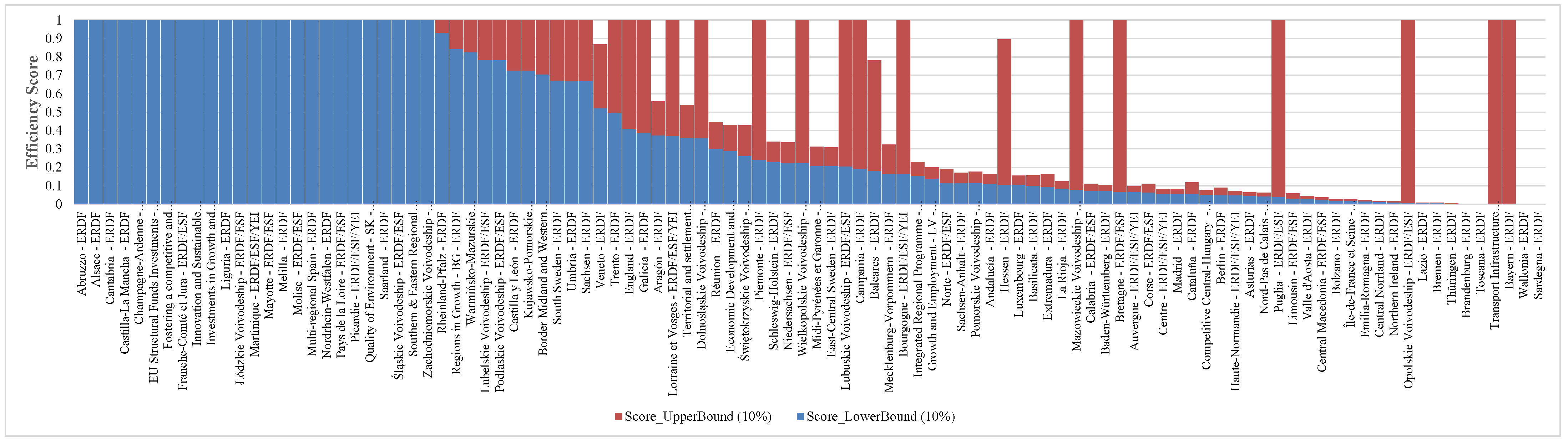
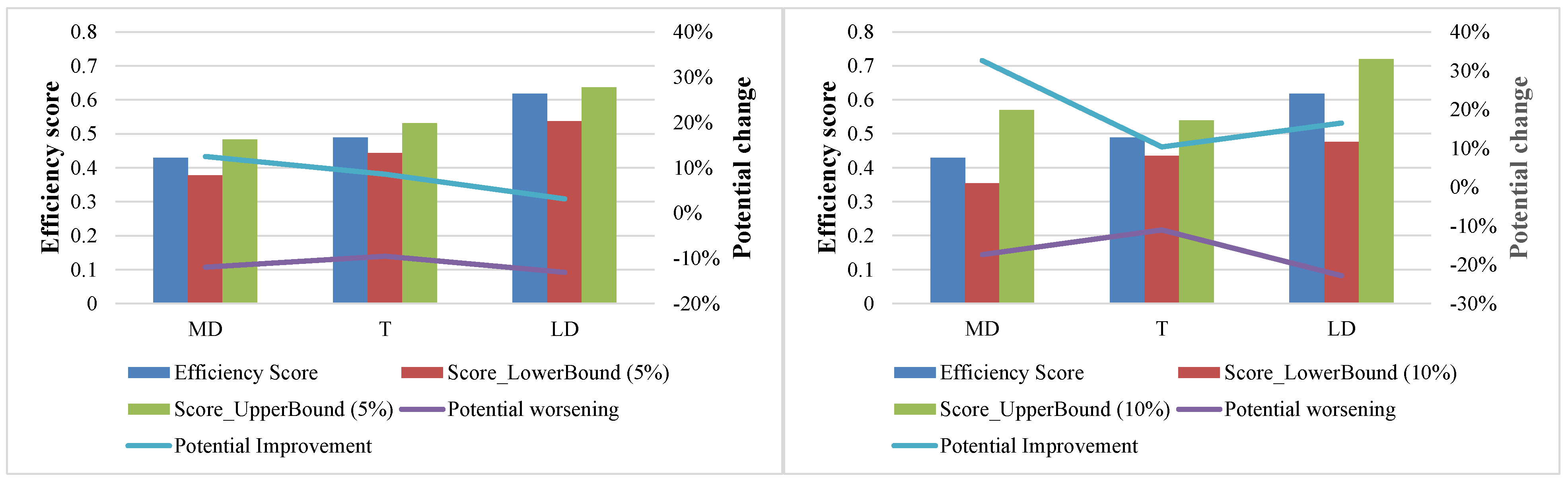
5.2. Robustness Analysis
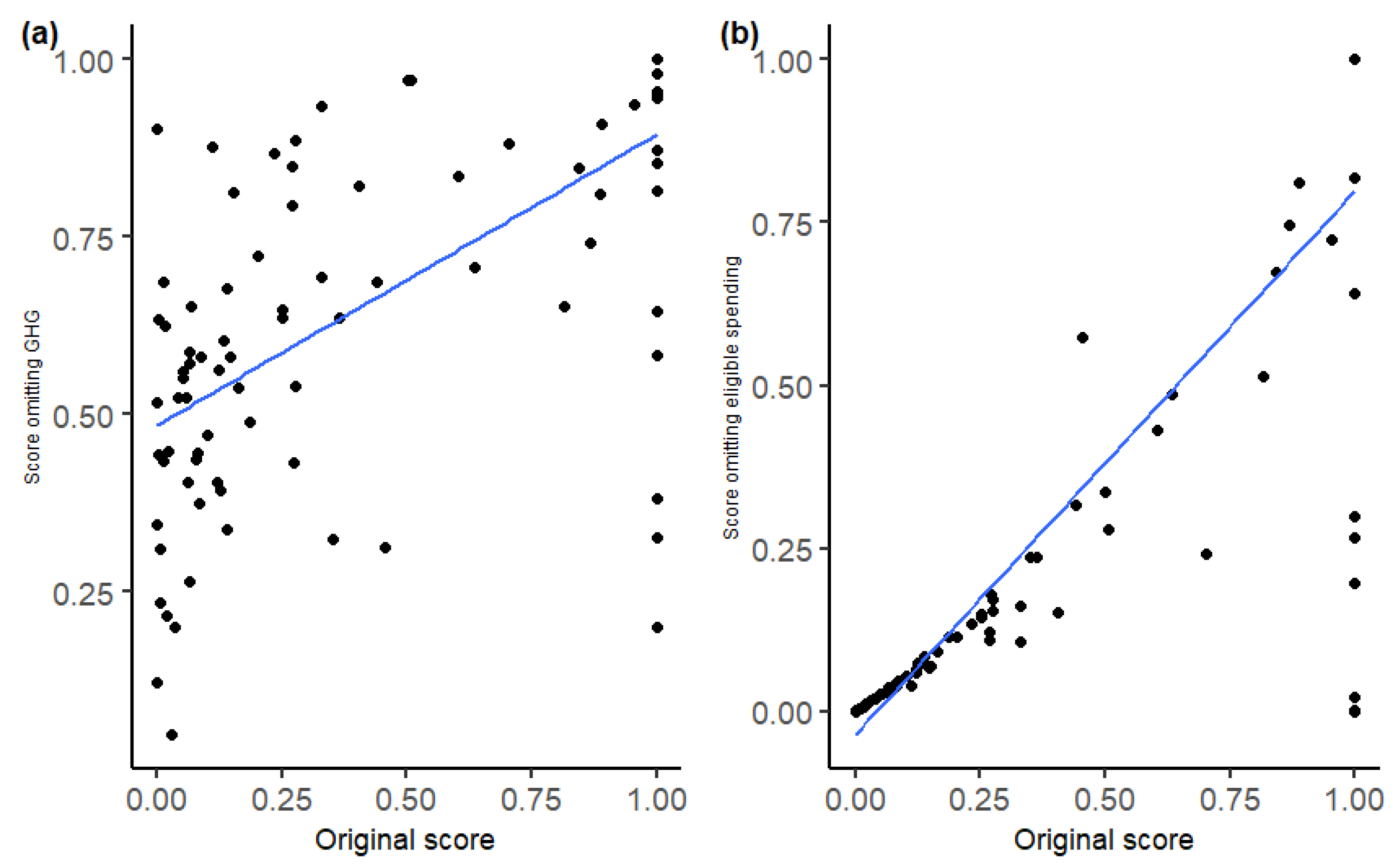
5.3. Sensitivity Analysis
5.4. Policy Implications
6. Conclusions
- (1)
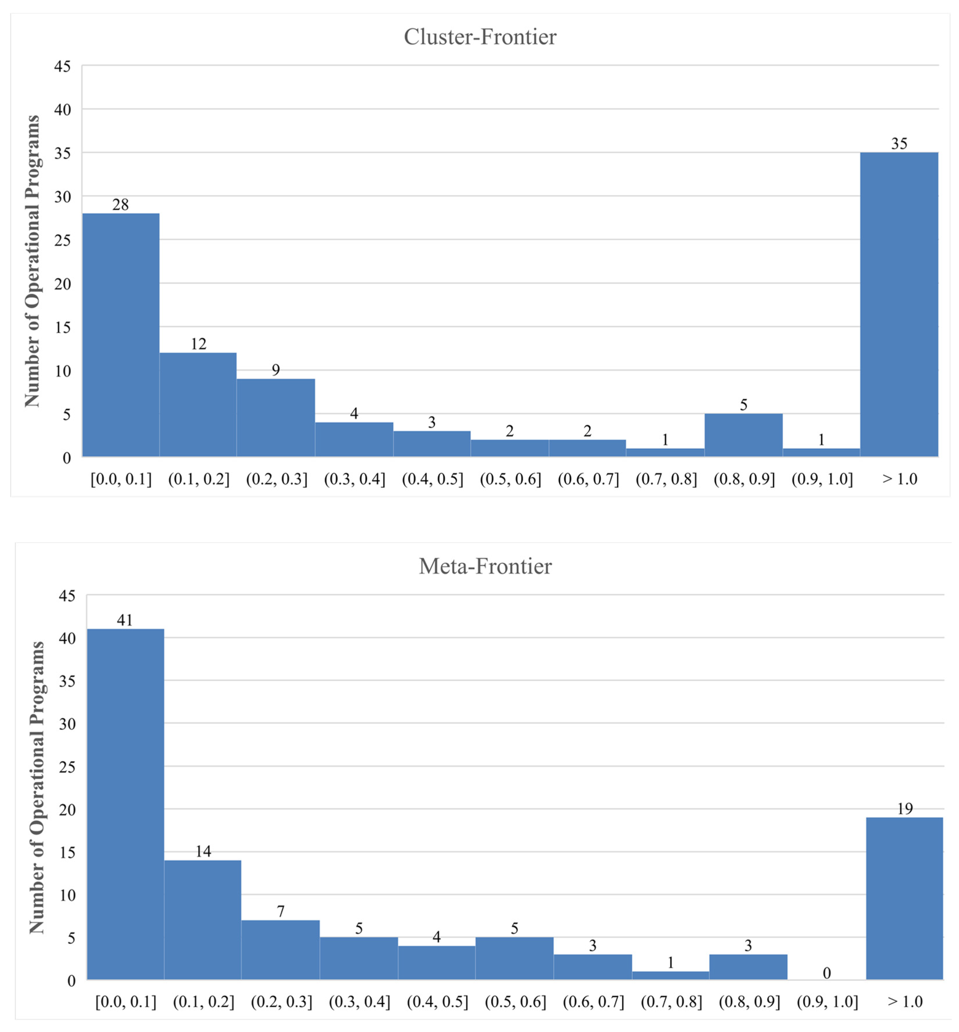
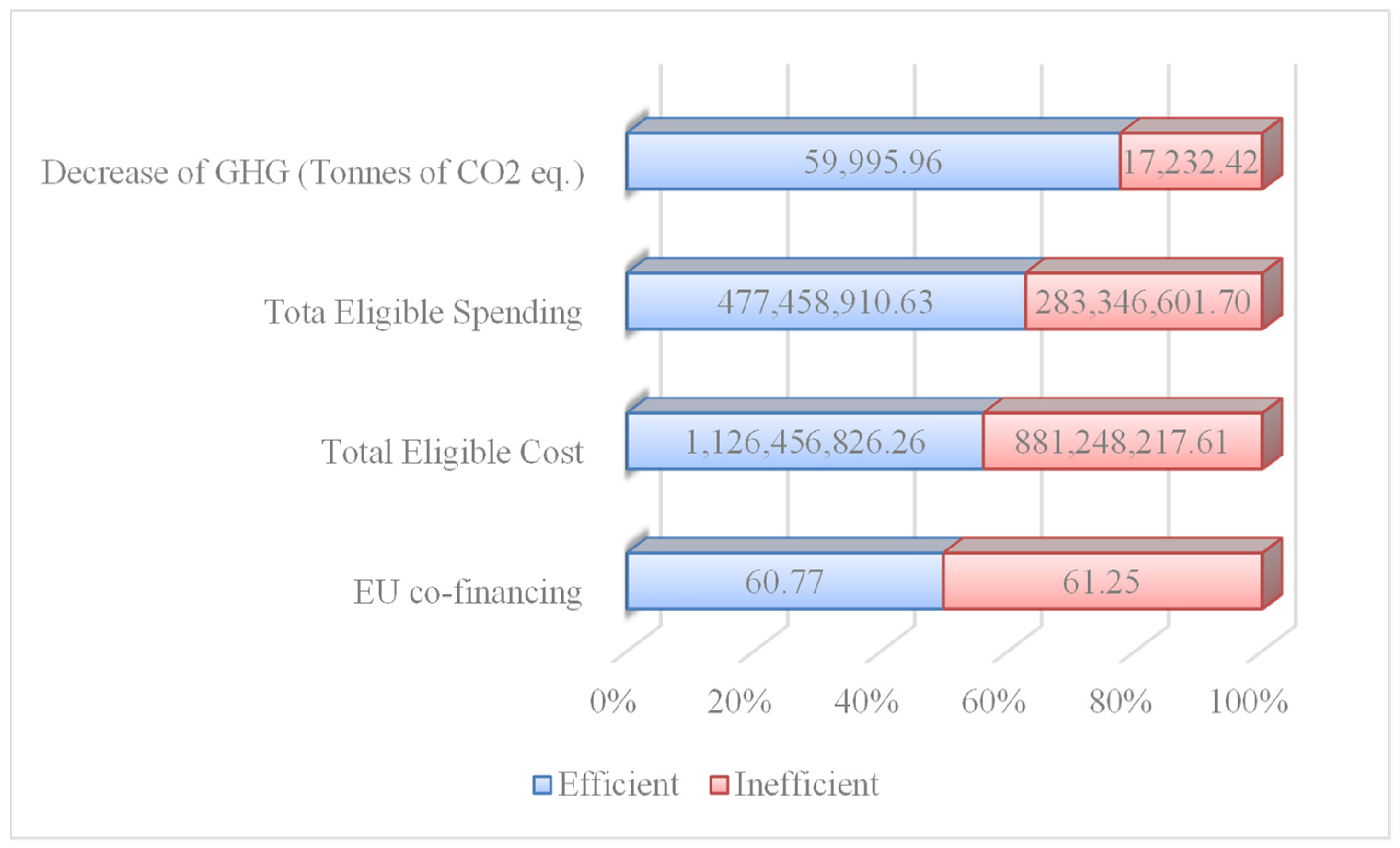
- MA should pay special attention to GHG emission reduction, since 59 OPs need to further improve their performance substantially. In such cases, consideration should be given to the prospect of replacing or supplementing these MAs with a capable alternative organization/group of experts, or perhaps providing particular training and exchanging best practices to improve the selection of projects for funding.
- (2)
- The other main important factor that precludes OPs’ efficiency is their implementation rate. Specifically, there are 11 OPs that have to more than double their performance and 7 who must enhance it by more than 75%. Either way, it is vital to understand the reasons behind these numbers. There are evaluation reports that suggest that some enterprises have withdrawn their subsidies, most likely due to issues related to bank credit. In this context, MA should be able to assist enterprises in obtaining other funding sources, while also easing the criteria for bringing in other institutional investors. Furthermore, in order to expedite the implementation of the OPs, best practices from other countries should be explored, and bureaucratic barriers to getting financing should be minimized. Management structures should seek ways to improve project implementation by supporting the simplification of procedures for submitting payment requests, also providing enhanced assistance and guidance.
- (1)
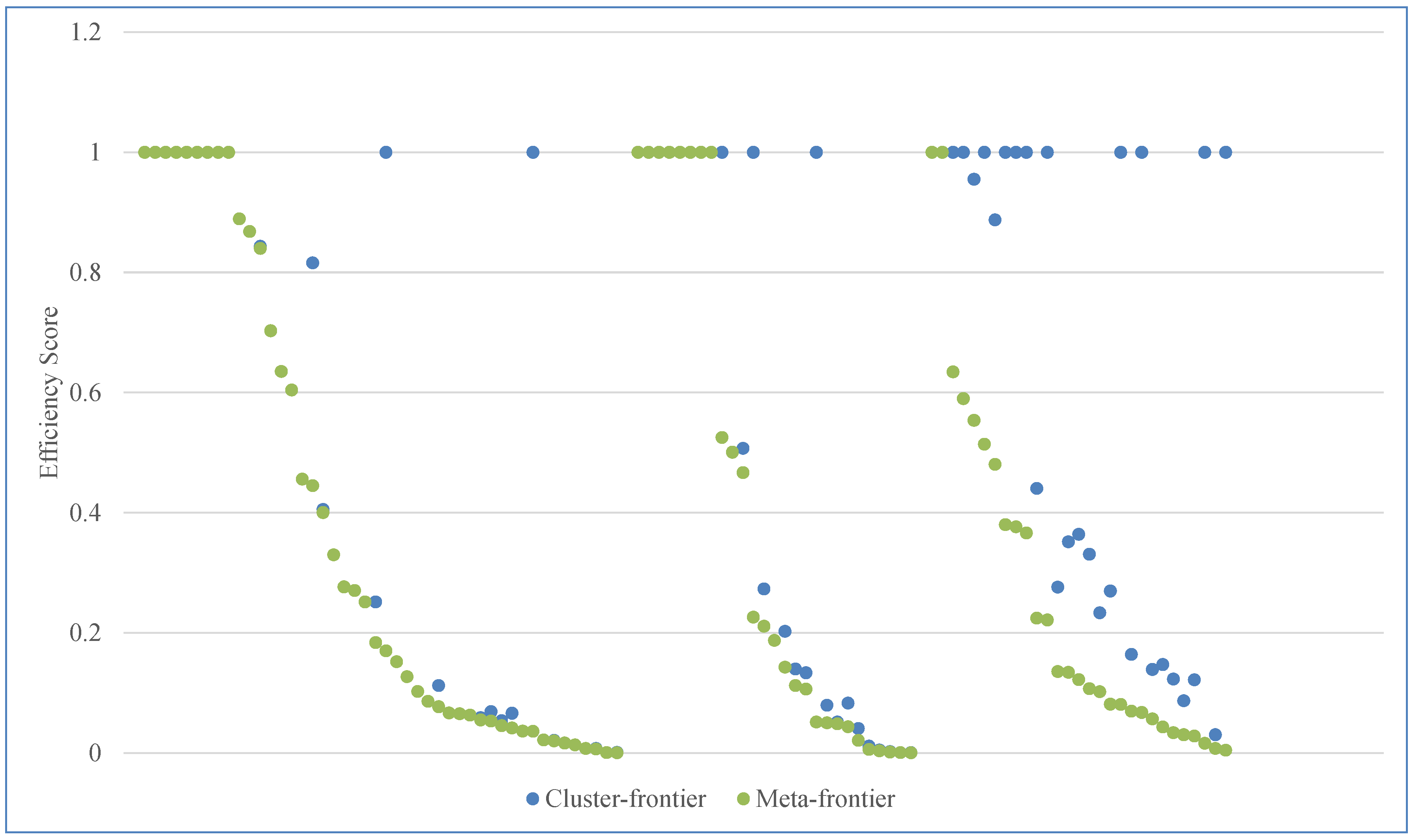
- The OPs more often viewed as benchmarks (either in the meta- or cluster frontiers) were, by decreasing order of importance, the “Southern and Eastern Regional Programme—IE—ERDF”, “Liguria—ERDF”, “Multi-regional Spain—ERDF”, “Pays de la Loire—ERDF/ESF”, “Investments in Growth and Employment—AT—ERDF and “Cantabria—ERDF”.
- (2)
- There is only one OP from a less developed region (see the case of Lithuania) that also serves as a benchmark (i.e., as a reference of best practices) for the other OPs in the meta-frontier (but just one time).
- (1)
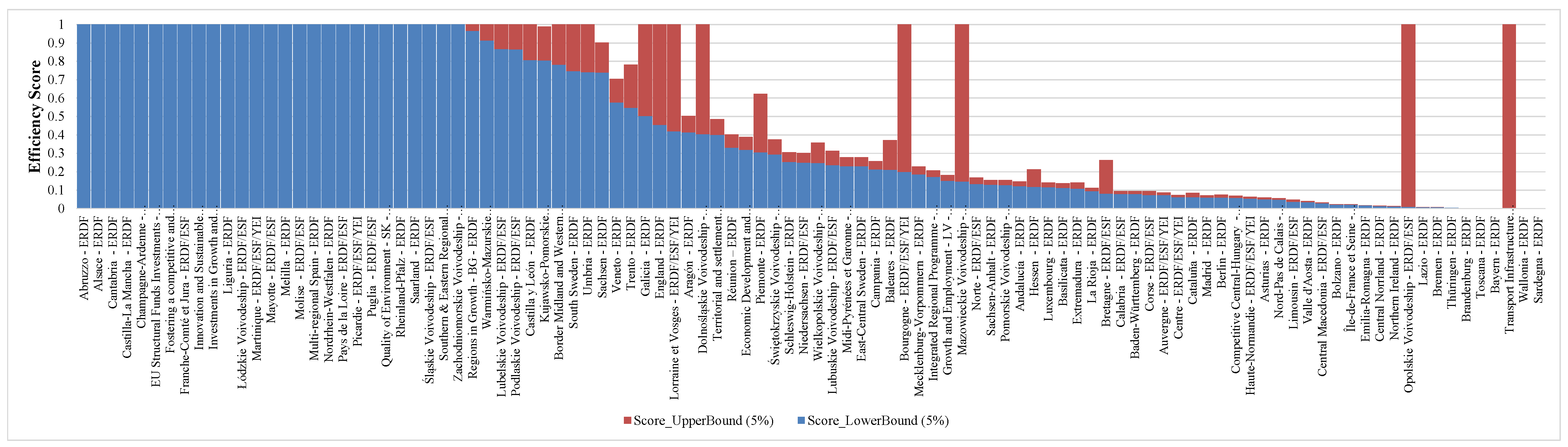
- 50% of LCE OPs were robustly inefficient for the tolerances considered in the analysis, highlighting the difficulty of further improving the efficiency of these OPs.
- (1)
- Our findings appear to support the apparent paradox of the EU Cohesion Policy, since the OPs which are more often viewed as benchmarks according to the meta-frontier belong to more developed regions. In fact, if we had not grouped our OPs according to the region type, we would only have 2 efficient OPs from the less developed regions (instead of the 13 obtained with the cluster frontier analysis).
- (2)
- The TGR reached by LCE OPs in less developed regions suggests that these produce, on average, only about 39.2%, of the potential output, given the technology available for this type of OPs in EU countries. Therefore, it appears that there is a positive association between the efficiency of the implementation of the OPs and the more advantageous socioeconomic circumstances of the regions where the OPs are implemented.
Author Contributions
Funding
Acknowledgments
Conflicts of Interest
Appendix A. Literature Review

| Title in English | Date of Publication | Authors | Methods (a) | ||||||||||
|---|---|---|---|---|---|---|---|---|---|---|---|---|---|
| DR | LR | MD/DA | I | FG/FW | S | CS | B | E | SM | O | |||
| Impact evaluation of the Alpine Space Interreg Operational Programme (OP), 2014–2020 | 1 February 2020 | t33 ([email protected]) | x | x | x | x | x | ||||||
| Evaluation of interventions to reduce CO2 emissions under the Investments in Growth and Employment OP, 2014–2020 | 1 June 2020 | Franziska Trebut and Gergard Bayer ([email protected]) | x | x | x | x | x | ||||||
| Preliminary evaluation of the implementation of territorial development under the Wallonia ERDF OP with a view to 2021–2027 | 1 March 2020 | Michaël Van Cutsem ([email protected]), Thomas Gayzal, Marie Gavroy, Clément Poulain | x | x | x | x | x | x | |||||
| Analysis of the market situation for Partnership Agreement (PA) 3—“Supporting the shift toward an LCE” of the future Technology and Applications for Competitiveness OP, 2021–2027, in the Czech Republic | 1 September 2020 | Deloitte Advisory s.r.o. (https://www2.deloitte.com/cz/, accessed on 19 November 2021) | x | x | x | ||||||||
| Evaluation of Specific Objectives 3.1, 3.2 and 3.4 of the Enterprise and Innovation for Competitiveness OP, 2014–2020 | 1 June 2019 | Asociace pro evropské fondy; EUFC CZ; Evaluation Advisory CE; enovation s.r.o.; SANCHO PANZA (www.apef.cz; www.eufc.cz; www.eace.cz; www.enovation.cz; www.sanchopanza.cz, accessed on 19 November 2021) | x | x | x | x | x | x | |||||
| Assessment of contribution of the Bayern OP, 2014–2020 to climate change objectives | 1 June 2019 | Entera—Thomas Horlitz ([email protected]) and Karoline Pawletko—Ramboll (www.de.ramboll.com, accessed on 19 November 2021) | x | x | x | x | x | x | |||||
| Evaluation of Priority Axis 3 “Reduction of CO2 emissions” in the ERDF Berlin OP 2014–2020 | 1 June 2019 | IfS—Institut für Stadtforschung und Strukturpolitik GmbH (www.ifsberlin.de, accessed on 19 November 2021); MR (www.mr-regionalberatung.de, accessed on 19 November 2021)—Gesellschaft für Regionalberatung mbH (Michael Ridder) | x | x | x | ||||||||
| Monitoring and evaluation of achievements in transition towards a low carbon economy | 1 January 2019 | Dirección General de Fondos Europeos SG de Programación y Evaluación (www.dgfc.sepg.hacienda.gob.es, accessed on 19 November 2021) | x | x | |||||||||
| Mid-term evaluation—the France-Belgium-Netherlands-UK (Two Seas) Interreg OP, 2014–2020 | 1 October 2019 | T33 Srl (www.t33.it, accessed on 19 November 2021, [email protected]) | x | x | x | x | |||||||
| Evaluation of the synergy and complementarity of the Bolzano EDRF OP 2014–2020 with the European Territorial Cooperation (ETC) OPs and programs directly managed by the EU | 1 December 2018 | CLAS (www.gruppoclas.com/it, accessed on 19 November 2021), PTS Group (www.ptsconsulting.it, accessed on 19 November 2021) and IRS—Istituto per la ricerca sociale (www.irsonline.it, accessed on 19 November 2021) | x | x | |||||||||
| Mid-term evaluation of the West-Nederland OP, 2014–2020: LCE | 1 October 2018 | Hans van der Zwan, Babette Beertema, William van den Bungelaar (www.erac.nl, accessed on 19 November 2021) | x | x | |||||||||
| Evaluation of the LCE priority under the Zuid-Nederland OP, 2014–2020 | 1 August 2018 | Andreas Ligtvoet, Annemieke van Barneveld-Biesma, Veerle Bastiaanssen, Alexander Buitenhuis, Chiel Scholten, Geert van der Veen (www.technopolis-group.com, accessed on 19 November 2021) | x | x | x | x | x | x | |||||
| Further analysis of low-carbon projects—Interim Evaluation Knowledge development and Innovation under the Noord and Oost-Nederland ERDF Ops, 2014–2020 | 1 March 2019 | Eelko Huizingh, Paul Elhorst, Evelien Croonen, Pedro de Faria, Anna-Lijsbeth Klijnstra (www.rug.nl, accessed on 19 November 2021) | x | x | x | x | |||||||
| Impact of cohesion policy 2007–2013 on energy in Poland | 1 April 2017 | FUNDEKO Korbel ([email protected]) | x | x | x | x | |||||||
| Improving energy efficiency in buildings in Małopolskie | 1 February 2018 | FUNDEKO Korbel ([email protected]) | x | x | x | ||||||||
| Evaluation of the criteria and system for selecting of projects within PA I and VII of the OP infrastructure and environment in Poland | 1 April 2017 | Zbigniew Dura, Marcin Pierzchała (IBC GROUP Central Europe Holding S. A., ul.) | x | x | x | x | x | ||||||
| Assessment of the energy advisory system for the public sector, housing and enterprises in the Infrastructure and Environment OP 2014–2020 | 1 December 2018 | Jan Frankowski, Magdalena Ośka, Andrzej Regulski, Henryk Kalinowski, Anna Matejczuk ([email protected], www.imapp.pl, accessed on 19 November 2021) | x | x | x | x | x | ||||||
| Evaluation of the contribution to the Sustainable Development Goals of the infrastructure and environment OPs 2007–2013 and 2014–2020 | 1 December 2018 | Michał Wolański, Paulina Kozłowska, Wiktor Mrozowski, Mateusz Pieróg, Maciej Pańczak (Wolański Ltd., ul. Stawki 8/7, 00-193 Warszawa, Poland) | x | x | x | x | x | x | x | ||||
| Evaluation of the effects of support for enterprises and their innovativeness and internationalization in Dolnośląskie in 2014–2020 | 1 June 2020 | Maciej Gajewski, Jan Szczucki, Robert Kubajek, Bogdan Pietrzak, Justyna Witkowska (www.pag-uniconsult.pl, accessed on 19 November 2021) | x | x | x | x | x | x | x | ||||
| Evaluation of measures for energy efficiency and the development of an LCE under the Warminsko-Mazurskie OP, 2014–2020 | 1 March 2021 | Openfield Sp. z o.o. (Ul. Ozimska 4/7, 45-0547 Opole) | x | x | x | x | x | x | x | ||||
| Evaluation of measures supporting the transition toward a low carbon economy Thematic Objective (TO) 4 in Portugal, 2014–2020 | 1 November 2020 | Heitor Gomes; Luís Carvalho; Sandra Primitivo ([email protected]) | x | x | x | x | x | x | |||||
| Evaluation of interventions to promote energy efficiency and carbon reduction under a regional OP in 2014–2020 | 1 May 2019 | Aurel Rizescu—Lattanzio Advisory Spa (www.lattanziokibs.com/ro, accessed on 19 November 2021) | x | x | x | x | x | x | |||||
| Impact evaluation of the Northern Periphery and Arctic Program 2014–2020: Final Report | 1 January 2018 | Irene McMaster, Nathalie Wergles and Heidi Vironen ([email protected]) | x | x | x | x | x | x | |||||
| Evaluation of the regional OPs, 2014–2020—regional analysis and national synthesis | 1 January 2019 | Sofia Nordmark and Lennart Svensson (University of Linköping) | x | x | x | x | x | ||||||
| Final report on the potential of the Green Fund (“Almi Invest Greentech”) to contribute to the transition to an LCE, 2014–2020 | 1 December 2019 | Sofia Avdeitchikova, Ylva Grauers Berggren, Elias Osvald and Klara Melin ([email protected]) | x | x | x | x | |||||||
| Evaluation of the 9 ERDF OPs, 2014–2020 supporting a shift towards an LCE | 1 July 2017 | Steffen Ovdahl ([email protected]), Stefan Wing, Robin Jacobsson, Sigfrid Grandström, Peter Sandén, and Charlotta Nicolaisen. | x | x | x | x | x | x | x | x | x | ||
| Internal evaluation of measurable indicators for the quality of environment OP, 2014–2020, in Slovakia | 1 June 2017 | Ministry of Environment of the Slovak Republic (www.minzp.sk, accessed on 19 November 2021) | x | x | |||||||||
Appendix B. Data
| Programme Title | EU Co-Financing | Total Eligible Cost | Total Eligible Spending | Decrease of GHG (Tonnes of CO2 eq.) | Category of Region |
|---|---|---|---|---|---|
| Abruzzo—ERDF | 50.00 | 58,435,905.16 | 23,573,823.75 | 2395.45 | Transition |
| Alsace—ERDF | 30.00 | 231,302,603.01 | 116,074,653.91 | 4619.91 | More Developed |
| Andalucía—ERDF | 80.00 | 1,276,301,168.05 | 375,799,945.48 | 13,490.54 | Transition |
| Aragón—ERDF | 50.00 | 94,346,366.93 | 20,258,377.22 | 17,416.41 | More Developed |
| Asturias—ERDF | 80.00 | 36,223,858.64 | 15,699,574.85 | 280.92 | More Developed |
| Auvergne—ERDF/ESF/YEI | 60.00 | 554,074,868.90 | 153,806,290.19 | 3705.07 | Transition |
| Baden-Württemberg—ERDF | 50.00 | 578,928,844.39 | 137,061,688.75 | 6900 | More Developed |
| Baleares—ERDF | 50.00 | 365,837,743.28 | 185,235,780.01 | 12,338.87 | More Developed |
| Basilicata—ERDF | 62.50 | 363,636,759.00 | 102,885,834.86 | 1737.06 | Less Developed |
| Bayern—ERDF | 35.99 | 1,489,123,542.01 | 656,914,176.00 | 15 | More Developed |
| Berlin—ERDF | 50.00 | 1,281,973,954.43 | 404,884,612.59 | 4801.22 | More Developed |
| Bolzano—ERDF | 50.00 | 223,357,744.90 | 64,933,239.72 | 757.45 | More Developed |
| Border Midland and Western Regional—ERDF | 50.00 | 288,733,916.00 | 137,473,567.01 | 62,380 | More Developed |
| Bourgogne—ERDF/ESF/YEI | 40.00 | 257,301,058.57 | 147,431,832.16 | 4654.36 | More Developed |
| Brandenburg—ERDF | 80.00 | 747,726,966.11 | 188,043,412.46 | 125 | Transition |
| Bremen—ERDF | 50.00 | 128,134,049.98 | 20,082,132.84 | 157.9 | More Developed |
| Bretagne—ERDF/ESF | 40.00 | 956,575,435.68 | 498,853,604.34 | 3924.45 | More Developed |
| Calabria—ERDF/ESF | 75.98 | 865,981,985.93 | 252,708,880.03 | 2895.64 | Less Developed |
| Campania—ERDF | 75.00 | 2,581,969,750.27 | 1,052,167,965.62 | 20,060.42 | Less Developed |
| Cantabria—ERDF | 50.00 | 17,878,192.28 | 17,139,539.60 | 3597.8 | More Developed |
| Castilla y León—ERDF | 50.00 | 27,077,783.86 | 20,792,431.41 | 5568.76 | More Developed |
| Castilla-La Mancha—ERDF | 80.00 | 32,425,249.29 | 10,736,556.62 | 11,489.61 | Transition |
| Cataluña—ERDF | 50.00 | 935,507,025.20 | 365,748,886.64 | 5213.55 | More Developed |
| Central Macedonia—ERDF/ESF | 80.00 | 217,029,604.29 | 5,547,887.69 | 269.03 | Less Developed |
| Central Norrland—ERDF | 50.00 | 66,633,992.00 | 20,547,144.00 | 145 | More Developed |
| Centre—ERDF/ESF/YEI | 50.00 | 68,076,791.12 | 12,795,310.28 | 774.3 | More Developed |
| Champagne-Ardenne—ERDF/ESF/YEI | 26.45 | 524,966,127.44 | 238,275,581.37 | 5558.7 | More Developed |
| Competitive Central-Hungary—ERDF/ESF | 50.00 | 565,656,554.27 | 144,222,696.95 | 4828.37 | More Developed |
| Corse—ERDF/ESF | 53.08 | 217,562,453.39 | 60,907,875.69 | 1536.2 | Transition |
| Dolnośląskie Voivodeship—ERDF/ESF | 85.00 | 2,077,483,889.94 | 1,001,921,517.85 | 35,353.57 | Less Developed |
| East-Central Sweden—ERDF | 50.00 | 167,300,046.00 | 69,896,525.00 | 8197 | More Developed |
| Economic Development and Innovation Programme—HU—ERDF/ESF/YEI | 85.00 | 521,361,163.21 | 87,075,491.77 | 10,935.64 | Less Developed |
| Emilia-Romagna—ERDF | 50.00 | 399,488,241.22 | 158,682,757.85 | 907.33 | More Developed |
| England—ERDF | 63.33 | 4,642,737,123.00 | 1,787,619,774.00 | 198,850.62 | Less Developed/More Developed/Transition |
| EU Structural Funds Investments—LT—ERDF/ESF/CF/YEI | 85.00 | 3,453,293,426.71 | 1,600,903,860.74 | 200,179 | Less Developed |
| Extremadura—ERDF | 80.00 | 221,014,003.31 | 46,630,594.02 | 990.03 | Less Developed |
| Fostering a competitive and sustainable economy—MT—ERDF/CF | 80.00 | 180,885,601.00 | 106,654,988.00 | 44,352.4 | Transition |
| Franche-Comté et Jura—ERDF/ESF | 40.03 | 526,812,648.08 | 341,537,370.99 | 9936.57 | Transition |
| Galicia—ERDF | 80.00 | 733,832,501.10 | 407,429,217.52 | 39,545.5 | More Developed |
| Growth and Employment—LV—ERDF/ESF/CF/YEI | 85.00 | 1,694,042,534.42 | 443,556,816.84 | 10,412.53 | Less Developed |
| Haute-Normandie—ERDF/ESF/YEI | 41.70 | 577,677,222.44 | 191,323,395.28 | 3218.18 | More Developed |
| Hessen—ERDF | 50.00 | 275,490,829.50 | 144,135,404.19 | 5525 | More Developed |
| Île-de-France et Seine—ESF/ERDF/YEI | 50.00 | 727,058,778.62 | 98,478,325.98 | 1762.45 | More Developed |
| Innovation and Sustainable Growth in Businesses—DK—ERDF | 55.00 | 264,194,402.53 | 55,493,280.74 | 51,005 | More Developed/Transition |
| Integrated Regional Programme—RO—ERDF | 82.50 | 6,832,205,666.95 | 1,154,004,429.05 | 81,269.68 | Less Developed/More Developed |
| Investments in Growth and Employment—AT—ERDF | 29.46 | 1,128,573,111.15 | 417,572,433.82 | 138,916.85 | Transition |
| Kujawsko-Pomorskie Voivodeship—ERDF/ESF | 85.00 | 1,506,750,014.59 | 597,254,294.00 | 83,139.53 | Less Developed |
| La Rioja—ERDF | 50.00 | 42,761,456.75 | 15,312,628.51 | 689.86 | More Developed |
| Lazio—ERDF | 50.00 | 852,677,890.23 | 164,496,345.48 | 618.37 | More Developed |
| Liguria—ERDF | 50.00 | 182,199,178.64 | 97,149,519.87 | 59,721.06 | More Developed |
| Limousin—ERDF/ESF | 50.63 | 320,053,393.93 | 107,841,896.93 | 950.03 | Transition |
| Łódzkie Voivodeship—ERDF/ESF | 85.00 | 197,418,057.95 | 20,551,342.65 | 15,622.52 | Less Developed |
| Lorraine et Vosges—ERDF/ESF/YEI | 60.00 | 1,656,282,325.56 | 743,909,207.67 | 64,087.69 | Transition |
| Lubelskie Voivodeship—ERDF/ESF | 85.00 | 2,504,075,733.48 | 1,013,421,268.71 | 155,491.65 | Less Developed |
| Lubuskie Voivodeship—ERDF/ESF | 85.00 | 564,061,137.01 | 247,835,390.66 | 5565.09 | Less Developed |
| Luxembourg—ERDF | 40.00 | 132,573,817.46 | 28,265,374.98 | 838 | More Developed |
| Madrid—ERDF | 50.00 | 247,674,348.76 | 91,485,646.80 | 2529.5 | More Developed |
| Martinique—ERDF/ESF/YEI | 51.89 | 368,436,576.30 | 137,487,602.99 | 24,578.38 | Less Developed |
| Mayotte—ERDF/ESF | 65.03 | 189,846,837.09 | 99,045,806.41 | 2147.7 | Less Developed |
| Mazowieckie Voivodeship—ERDF/ESF | 80.00 | 2,145,555,296.34 | 1,006,723,930.61 | 3674.43 | More Developed |
| Mecklenburg-Vorpommern—ERDF | 80.00 | 789,161,637.01 | 317,802,200.05 | 13,824 | Transition |
| Melilla—ERDF | 80.00 | 32,171,439.92 | 27,959,444.29 | 3114.94 | Transition |
| Midi-Pyrénées et Garonne—ERDF/ESF/YEI | 38.23 | 810,136,128.58 | 330,097,528.66 | 12,915.45 | More Developed |
| Molise—ERDF/ESF | 55.00 | 39,965,455.00 | 8,325,490.89 | 328.3 | Transition |
| Multi-regional Spain—ERDF | 72.47 | 5,460,800,959.76 | 2,196,113,419.20 | 713,649.45 | Less Developed/More Developed/Transition |
| Niedersachsen—ERDF/ESF | 51.88 | 1,195,970,497.97 | 255,728,896.81 | 29,451.4 | Transition |
| Nord-Pas de Calais—ERDF/ESF/YEI | 48.86 | 2,295,271,228.26 | 546,428,560.00 | 8067.15 | Transition |
| Nordrhein-Westfalen—ERDF | 50.00 | 2,646,766,161.98 | 1,087,091,636.85 | 32,137.3 | More Developed |
| Norte—ERDF/ESF | 84.43 | 444,612,989.40 | 133,529,560.49 | 2648.16 | Less Developed |
| Northern Ireland—ERDF | 60.00 | 305,856,240.00 | 138,042,805.05 | 250 | Transition |
| Opolskie Voivodeship—ERDF/ESF | 85.00 | 773,590,071.60 | 399,584,835.80 | 218 | Less Developed |
| Pays de la Loire—ERDF/ESF | 27.41 | 833,267,673.38 | 523,893,731.83 | 16,470.43 | More Developed |
| Picardie—ERDF/ESF/YEI | 22.31 | 1,270,962,446.12 | 307,379,379.83 | 26,725.25 | More Developed/Transition |
| Piemonte—ERDF | 50.00 | 738,745,949.77 | 382,614,685.69 | 24,817.83 | More Developed |
| Podlaskie Voivodeship—ERDF/ESF | 85.00 | 1,002,566,230.14 | 473,030,923.16 | 54,876.63 | Less Developed |
| Pomorskie Voivodeship—ERDF/ESF | 85.00 | 1,486,316,708.43 | 494,299,792.10 | 7608.52 | Less Developed |
| Puglia—ERDF/ESF | 57.50 | 559,318,475.94 | 276,518,084.10 | 825.18 | Less Developed |
| Quality of Environment—SK—ERDF/CF | 60.74 | 3,268,602,896.66 | 1,497,980,442.01 | 143,827.12 | Less Developed |
| Regions in Growth—BG—ERDF | 85.00 | 576,761,289.61 | 292,362,688.54 | 32,926.77 | Less Developed |
| Réunion—ERDF | 58.40 | 782,421,299.34 | 240,342,060.27 | 11,874.11 | Less Developed |
| Rheinland-Pfalz—ERDF | 29.75 | 685,461,896.34 | 404,698,111.76 | 36,084.45 | More Developed |
| Saarland—ERDF | 39.03 | 136,365,278.30 | 69,140,448.05 | 9409 | More Developed |
| Sachsen—ERDF | 80.00 | 1,601,931,420.46 | 525,168,561.95 | 83,549.03 | More Developed |
| Sachsen-Anhalt—ERDF | 74.06 | 1,227,541,432.93 | 203,679,210.16 | 14,923.22 | Transition |
| Sardegna—ERDF | 50.00 | 768,276,720.88 | 223,563,933.80 | 20.64 | Transition |
| Schleswig-Holstein—ERDF | 50.00 | 253,158,401.59 | 88,233,312.12 | 12,939 | More Developed |
| Śląskie Voivodeship—ERDF/ESF | 85.00 | 617,775,673.81 | 104,185,493.52 | 55,332.55 | Less Developed |
| South Sweden—ERDF | 50.00 | 73,647,631.00 | 30,233,182.00 | 23,454 | More Developed |
| Southern and Eastern Regional Programme—IE—ERDF | 50.00 | 643,878,121.00 | 262,200,018.97 | 162,937 | More Developed |
| Świętokrzyskie Voivodeship—ERDF/ESF | 85.00 | 671,027,980.84 | 240,385,684.51 | 9459.71 | Less Developed |
| Territorial and settlement Development—HU—ERDF/ESF | 85.00 | 2,956,091,946.73 | 950,777,469.67 | 55,774.05 | Less Developed |
| Thüringen—ERDF | 80.00 | 1,036,387,583.36 | 337,366,169.48 | 358.6 | Transition |
| Toscana—ERDF | 50.00 | 943,317,579.60 | 69,225,135.69 | 55.05 | More Developed |
| Transport Infrastructure Environment and Sustainable Development—GR—ERDF/CF | 80.00 | 6,412,116,038.24 | 2,362,923,936.48 | 199 | Less Developed/More Developed/Transition |
| Trento—ERDF | 50.00 | 48,212,037.23 | 30,098,971.29 | 6202 | More Developed |
| Umbria—ERDF | 50.00 | 105,098,679.13 | 60,443,437.21 | 22,868.39 | More Developed |
| Valle d’Aosta—ERDF | 50.00 | 49,066,309.27 | 7,342,763.33 | 285.9 | More Developed |
| Veneto—ERDF | 50.00 | 221,403,382.53 | 101,376,473.12 | 33,354.22 | More Developed |
| Wallonia—ERDF | 40.00 | 1,246,557,134.92 | 193,582,687.49 | 37.16 | More Developed/Transition |
| Warmińsko-Mazurskie Voivodeship—ERDF/ESF | 85.00 | 1,159,197,959.15 | 550,551,004.38 | 68,741.28 | Less Developed |
| Wielkopolskie Voivodeship—ERDF/ESF | 85.00 | 2,014,023,770.84 | 861,478,246.23 | 19,997.43 | Less Developed |
| Zachodniomorskie Voivodeship—ERDF/ESF | 85.00 | 151,556,615.01 | 5,657,445.00 | 4837.92 | Less Developed |
Appendix C. Results
| DMU | Cluster | Score | Benchmark (Lambda) | Projection (EU Co-Financing) | Projection (Total Eligible Cost) | Projection (Total Eligible Spending) | Projection (Decrease of GHG (Tonnes of CO2 eq.) |
|---|---|---|---|---|---|---|---|
| Abruzzo—ERDF | MD | 1.00 | Abruzzo—ERDF(1.000000) | 50.00 | 58,435,905.16 | 23,573,823.75 | 2395.45 |
| Alsace—ERDF | T | 1.00 | Alsace—ERDF(1.000000) | 30.00 | 231,302,603.01 | 116,074,653.91 | 4619.91 |
| Andalucía—ERDF | MD | 0.13 | Fostering a competitive and sustainable economy—MT—ERDF/CF(0.792532); Multi-regional Spain—ERDF(0.207468) | 78.44 | 1,276,301,168.05 | 540,151,575.87 | 183,210.38 |
| Aragón—ERDF | T | 0.46 | Cantabria—ERDF(0.534641); Liguria—ERDF(0.465359) | 50.00 | 94,346,366.93 | 54,372,867.37 | 29,715.24 |
| Asturias—ERDF | T | 0.05 | Cantabria—ERDF(0.671044); South Sweden—ERDF(0.328956) | 50.00 | 36,223,858.64 | 21,446,765.93 | 10,129.61 |
| Auvergne—ERDF/ESF/YEI | MD | 0.08 | Fostering a competitive and sustainable economy—MT—ERDF/CF(0.159244); Innovation and Sustainable Growth in Businesses—DK—ERDF(0.782421); Multi-regional Spain—ERDF(0.058336) | 60.00 | 554,074,868.90 | 188,514,714.21 | 88,601.34 |
| Baden-Württemberg—ERDF | T | 0.09 | Liguria—ERDF(0.140681); Southern and Eastern Regional Programme—IE—ERDF(0.859319) | 50.00 | 578,928,844.39 | 238,980,613.58 | 148,416.52 |
| Baleares—ERDF | T | 0.27 | Liguria—ERDF(0.649681); Pays de la Loire—ERDF/ESF(0.115654); Southern and Eastern Regional Programme—IE—ERDF(0.234665) | 47.39 | 365,837,743.28 | 185,235,780.01 | 78,940.11 |
| Basilicata—ERDF | LD | 0.12 | Łódzkie Voivodeship—ERDF/ESF(0.201495); Martinique—ERDF/ESF/YEI(0.679553); Śląskie Voivodeship—ERDF/ESF(0.118952) | 62.50 | 363,636,759.00 | 109,964,213.88 | 26,432.11 |
| Bayern—ERDF | T | 0.00 | Nordrhein-Westfalen—ERDF(0.281744); Pays de la Loire—ERDF/ESF(0.620215); Southern and Eastern Regional Programme—IE—ERDF(0.098042) | 35.99 | 1,325,641,058.21 | 656,914,176.00 | 35,244.32 |
| Berlin—ERDF | T | 0.07 | Nordrhein-Westfalen—ERDF(0.172974); Southern and Eastern Regional Programme—IE—ERDF(0.827026) | 50.00 | 990,325,169.31 | 404,884,612.59 | 140,312.09 |
| Bolzano—ERDF | T | 0.02 | Liguria—ERDF(0.910850); Southern and Eastern Regional Programme—IE—ERDF(0.089150) | 50.00 | 223,357,744.90 | 111,863,732.02 | 68,922.74 |
| Border Midland and Western Regional—ERDF | T | 0.87 | Liguria—ERDF(0.773977); Pays de la Loire—ERDF/ESF(0.011536); Southern and Eastern Regional Programme—IE—ERDF(0.214487) | 49.74 | 288,733,916.00 | 137,473,567.01 | 81,360.59 |
| Bourgogne—ERDF/ESF/YEI | T | 0.33 | Alsace—ERDF(0.008601); Liguria—ERDF(0.260278); Pays de la Loire—ERDF/ESF(0.155244); Saarland—ERDF(0.575877) | 40.00 | 257,301,058.57 | 147,431,832.16 | 23,559.19 |
| Brandenburg—ERDF | MD | 0.00 | Fostering a competitive and sustainable economy—MT—ERDF/CF(0.892642); Multi-regional Spain—ERDF(0.107358) | 79.19 | 747,726,966.11 | 330,975,150.16 | 116,206.82 |
| Bremen—ERDF | T | 0.01 | Liguria—ERDF(0.501941); South Sweden—ERDF(0.498059) | 50.00 | 128,134,049.98 | 63,821,202.63 | 41,657.91 |
| Bretagne—ERDF/ESF | T | 0.11 | Mazowieckie Voivodeship—ERDF/ESF(0.071822); Nordrhein-Westfalen—ERDF(0.051408); Pays de la Loire—ERDF/ESF(0.537936); Southern and Eastern Regional Programme—IE—ERDF(0.338834) | 40.00 | 956,575,435.68 | 498,853,604.34 | 65,984.71 |
| Calabria—ERDF/ESF | LD | 0.09 | Lubelskie Voivodeship—ERDF/ESF(0.167584); Martinique—ERDF/ESF/YEI(0.272350); Śląskie Voivodeship—ERDF/ESF(0.560066) | 75.98 | 865,981,985.93 | 265,628,702.94 | 63,741.72 |
| Campania—ERDF | LD | 0.23 | EU Structural Funds Investments—LT—ERDF/ESF/CF/YEI(0.690196); Martinique—ERDF/ESF/YEI(0.280710); Quality of Environment—SK—ERDF/CF(0.029094) | 75.00 | 2,581,969,750.27 | 1,187,113,772.18 | 149,246.65 |
| Cantabria—ERDF | T | 1.00 | Cantabria—ERDF(1.000000) | 50.00 | 17,878,192.28 | 17,139,539.60 | 3597.80 |
| Castilla y León—ERDF | T | 0.89 | Cantabria—ERDF(0.944015); Liguria—ERDF(0.055985) | 50.00 | 27,077,783.86 | 21,618,937.86 | 6739.89 |
| Castilla-La Mancha—ERDF | MD | 1.00 | Castilla-La Mancha—ERDF(1.000000) | 80.00 | 32,425,249.29 | 10,736,556.62 | 11,489.61 |
| Cataluña—ERDF | T | 0.07 | Nordrhein-Westfalen—ERDF(0.125530); Southern and Eastern Regional Programme—IE—ERDF(0.874470) | 50.00 | 895,301,197.95 | 365,748,886.64 | 146,517.68 |
| Central Macedonia—ERDF/ESF | LD | 0.03 | Łódzkie Voivodeship—ERDF/ESF(0.826714); Martinique—ERDF/ESF/YEI(0.117160); Mayotte—ERDF/ESF(0.056126) | 80.00 | 217,029,604.29 | 38,657,163.22 | 15,915.50 |
| Central Norrland—ERDF | T | 0.01 | Cantabria—ERDF(0.125761); South Sweden—ERDF(0.874239) | 50.00 | 66,633,992.00 | 28,586,508.07 | 20,956.86 |
| Centre—ERDF/ESF/YEI | T | 0.07 | Cantabria—ERDF(0.694509); Liguria—ERDF(0.305491) | 50.00 | 68,076,791.12 | 41,581,876.47 | 20,742.96 |
| Champagne-Ardenne—ERDF/ESF/YEI | T | 1.00 | Champagne-Ardenne—ERDF/ESF/YEI(1.000000) | 26.45 | 524,966,127.44 | 238,275,581.37 | 5558.70 |
| Competitive Central-Hungary—ERDF/ESF | T | 0.06 | Liguria—ERDF(0.169428); Southern and Eastern Regional Programme—IE—ERDF(0.830572) | 50.00 | 565,656,554.27 | 234,235,761.90 | 145,449.28 |
| Corse—ERDF/ESF | MD | 0.08 | Abruzzo—ERDF(0.388718); Fostering a competitive and sustainable economy—MT—ERDF/CF(0.044763); Innovation and Sustainable Growth in Businesses—DK—ERDF(0.523622); Investments in Growth and Employment—AT—ERDF(0.042897) | 53.08 | 217,562,453.39 | 60,907,875.69 | 35,582.95 |
| Dolnośląskie Voivodeship—ERDF/ESF | LD | 1.00 | Dolnośląskie Voivodeship—ERDF/ESF(1.000000) | 85.00 | 2,077,483,889.94 | 1,001,921,517.85 | 35,353.57 |
| East-Central Sweden—ERDF | T | 0.25 | Cantabria—ERDF(0.090671); Liguria—ERDF(0.909329) | 50.00 | 167,300,046.00 | 89,894,942.50 | 54,632.31 |
| Economic Development and Innovation Programme—HU—ERDF/ESF/YEI | LD | 0.35 | Martinique—ERDF/ESF/YEI(0.265932); Regions in Growth—BG—ERDF(0.734068) | 76.20 | 521,361,163.21 | 251,176,507.70 | 30,706.67 |
| Emilia-Romagna—ERDF | T | 0.02 | Liguria—ERDF(0.529350); Southern and Eastern Regional Programme—IE—ERDF(0.470650) | 50.00 | 399,488,241.22 | 174,830,490.21 | 108,299.61 |
| England—ERDF | MD | 0.50 | Investments in Growth and Employment—AT—ERDF(0.074491); Multi-regional Spain—ERDF(0.807282); Picardie—ERDF/ESF/YEI(0.118227) | 63.33 | 4,642,737,123.00 | 1,840,328,863.93 | 589,624.10 |
| EU Structural Funds Investments—LT—ERDF/ESF/CF/YEI | LD | 1.00 | EU Structural Funds Investments—LT—ERDF/ESF/CF/YEI(1.000000) | 85.00 | 3,453,293,426.71 | 1,600,903,860.74 | 200,179.00 |
| Extremadura—ERDF | LD | 0.12 | Łódzkie Voivodeship—ERDF/ESF(0.737905); Martinique—ERDF/ESF/YEI(0.143235); Mayotte—ERDF/ESF(0.118860) | 77.88 | 221,014,003.31 | 46,630,594.02 | 15,303.69 |
| Fostering a competitive and sustainable economy—MT—ERDF/CF | MD | 1.00 | Fostering a competitive and sustainable economy—MT—ERDF/CF(1.000000) | 80.00 | 180,885,601.00 | 106,654,988.00 | 44,352.40 |
| Franche-Comté et Jura—ERDF/ESF | MD | 1.00 | Franche-Comté et Jura—ERDF/ESF(1.000000) | 40.03 | 526,812,648.08 | 341,537,370.99 | 9936.57 |
| Galicia—ERDF | T | 0.70 | Liguria—ERDF(0.044265); Pays de la Loire—ERDF/ESF(0.582877); Southern and Eastern Regional Programme—IE—ERDF(0.372858) | 36.83 | 733,832,501.10 | 407,429,217.52 | 72,996.11 |
| Growth and Employment—LV—ERDF/ESF/CF/YEI | LD | 0.16 | Lubelskie Voivodeship—ERDF/ESF(0.570570); Śląskie Voivodeship—ERDF/ESF(0.429430) | 85.00 | 1,694,042,534.42 | 622,968,456.13 | 112,480.36 |
| Haute-Normandie—ERDF/ESF/YEI | T | 0.06 | Alsace—ERDF(0.077960); Champagne-Ardenne—ERDF/ESF/YEI(0.286234); Southern and Eastern Regional Programme—IE—ERDF(0.635806) | 41.70 | 577,677,222.44 | 243,960,145.39 | 105,547.66 |
| Hessen—ERDF | T | 0.15 | Liguria—ERDF(0.826761); Pays de la Loire—ERDF/ESF(0.070283); Southern and Eastern Regional Programme—IE—ERDF(0.102955) | 48.41 | 275,490,829.50 | 144,135,404.19 | 67,307.89 |
| Île-de-France et Seine—ESF/ERDF/YEI | T | 0.02 | Southern and Eastern Regional Programme—IE—ERDF(1.000000) | 50.00 | 643,878,121.00 | 262,200,018.97 | 162,937.00 |
| Innovation and Sustainable Growth in Businesses—DK—ERDF | MD | 1.00 | Innovation and Sustainable Growth in Businesses—DK—ERDF(1.000000) | 55.00 | 264,194,402.53 | 55,493,280.74 | 51,005.00 |
| Integrated Regional Programme—RO—ERDF | MD | 0.19 | Multi-regional Spain—ERDF(1.000000) | 72.47 | 5,460,800,959.76 | 2,196,113,419.20 | 713,649.45 |
| Investments in Growth and Employment—AT—ERDF | MD | 1.00 | Investments in Growth and Employment—AT—ERDF(1.000000) | 29.46 | 1,128,573,111.15 | 417,572,433.82 | 138,916.85 |
| Kujawsko-Pomorskie Voivodeship—ERDF/ESF | LD | 0.89 | EU Structural Funds Investments—LT—ERDF/ESF/CF/YEI(0.151499); Warmińsko-Mazurskie Voivodeship—ERDF/ESF(0.848501) | 85.00 | 1,506,750,014.59 | 709,677,901.81 | 88,653.90 |
| La Rioja—ERDF | T | 0.10 | Cantabria—ERDF(0.553819); South Sweden—ERDF(0.446181) | 50.00 | 42,761,456.75 | 22,981,674.18 | 12,457.26 |
| Lazio—ERDF | T | 0.01 | Southern and Eastern Regional Programme—IE—ERDF(1.000000) | 50.00 | 643,878,121.00 | 262,200,018.97 | 162,937.00 |
| Liguria—ERDF | T | 1.00 | Liguria—ERDF(1.000000) | 50.00 | 182,199,178.64 | 97,149,519.87 | 59,721.06 |
| Limousin—ERDF/ESF | MD | 0.04 | Abruzzo—ERDF(0.407498); Fostering a competitive and sustainable economy—MT—ERDF/CF(0.079419); Innovation and Sustainable Growth in Businesses—DK—ERDF(0.343803); Investments in Growth and Employment—AT—ERDF(0.169279) | 50.63 | 320,053,393.93 | 107,841,896.93 | 45,550.01 |
| Łódzkie Voivodeship—ERDF/ESF | LD | 1.00 | Łódzkie Voivodeship—ERDF/ESF(1.000000) | 85.00 | 197,418,057.95 | 20,551,342.65 | 15,622.52 |
| Lorraine et Vosges—ERDF/ESF/YEI | MD | 0.51 | Fostering a competitive and sustainable economy—MT—ERDF/CF(0.211438); Franche-Comté et Jura—ERDF/ESF(0.544821); Multi-regional Spain—ERDF(0.243740) | 56.39 | 1,656,282,325.56 | 743,909,207.67 | 188,736.60 |
| Lubelskie Voivodeship—ERDF/ESF | LD | 1.00 | Lubelskie Voivodeship—ERDF/ESF(1.000000) | 85.00 | 2,504,075,733.48 | 1,013,421,268.71 | 155,491.65 |
| Lubuskie Voivodeship—ERDF/ESF | LD | 0.27 | Martinique—ERDF/ESF/YEI(0.092552); Regions in Growth—BG—ERDF(0.746997); Śląskie Voivodeship—ERDF/ESF(0.160451) | 81.94 | 564,061,137.01 | 247,835,390.66 | 35,749.14 |
| Luxembourg—ERDF | T | 0.13 | Liguria—ERDF(0.016400); Saarland—ERDF(0.911162); South Sweden—ERDF(0.072438) | 40.00 | 132,573,817.46 | 66,781,434.77 | 11,251.52 |
| Madrid—ERDF | T | 0.07 | Liguria—ERDF(0.858180); Southern and Eastern Regional Programme—IE—ERDF(0.141820) | 50.00 | 247,674,348.76 | 120,556,932.50 | 74,359.11 |
| Martinique—ERDF/ESF/YEI | LD | 1.00 | Martinique—ERDF/ESF/YEI(1.000000) | 51.89 | 368,436,576.30 | 137,487,602.99 | 24,578.38 |
| Mayotte—ERDF/ESF | LD | 1.00 | Mayotte—ERDF/ESF(1.000000) | 65.03 | 189,846,837.09 | 99,045,806.41 | 2147.70 |
| Mazowieckie Voivodeship—ERDF/ESF | T | 1.00 | Mazowieckie Voivodeship—ERDF/ESF(1.000000) | 80.00 | 2,145,555,296.34 | 1,006,723,930.61 | 3674.43 |
| Mecklenburg-Vorpommern—ERDF | MD | 0.20 | Fostering a competitive and sustainable economy—MT—ERDF/CF(0.884794); Multi-regional Spain—ERDF(0.115206) | 79.13 | 789,161,637.01 | 347,372,386.97 | 121,459.20 |
| Melilla—ERDF | MD | 1.00 | Melilla—ERDF(1.000000) | 80.00 | 32,171,439.92 | 27,959,444.29 | 3114.94 |
| Midi-Pyrénées et Garonne—ERDF/ESF/YEI | T | 0.25 | Rheinland-Pfalz—ERDF(0.581481); Southern and Eastern Regional Programme—IE—ERDF(0.418519) | 38.23 | 668,058,316.29 | 345,060,021.07 | 89,174.59 |
| Molise—ERDF/ESF | MD | 1.00 | Molise—ERDF/ESF(1.000000) | 55.00 | 39,965,455.00 | 8,325,490.89 | 328.30 |
| Multi-regional Spain—ERDF | MD | 1.00 | Multi-regional Spain—ERDF(1.000000) | 72.47 | 5,460,800,959.76 | 2,196,113,419.20 | 713,649.45 |
| Niedersachsen—ERDF/ESF | MD | 0.27 | Innovation and Sustainable Growth in Businesses—DK—ERDF(0.637307); Investments in Growth and Employment—AT—ERDF(0.219978); Multi-regional Spain—ERDF(0.142715) | 51.88 | 1,195,970,497.97 | 440,640,545.66 | 164,912.73 |
| Nord-Pas de Calais—ERDF/ESF/YEI | MD | 0.05 | Innovation and Sustainable Growth in Businesses—DK—ERDF(0.229098); Investments in Growth and Employment—AT—ERDF(0.455885); Multi-regional Spain—ERDF(0.315017) | 48.86 | 2,295,271,228.26 | 894,891,523.90 | 299,826.97 |
| Nordrhein-Westfalen—ERDF | T | 1.00 | Nordrhein-Westfalen—ERDF(1.000000) | 50.00 | 2,646,766,161.98 | 1,087,091,636.85 | 32,137.30 |
| Norte—ERDF/ESF | LD | 0.15 | Martinique—ERDF/ESF/YEI(0.688890); Regions in Growth—BG—ERDF(0.034024); Śląskie Voivodeship—ERDF/ESF(0.277086) | 62.19 | 444,612,989.40 | 133,529,560.49 | 33,383.97 |
| Northern Ireland—ERDF | MD | 0.01 | Abruzzo—ERDF(0.340753); Fostering a competitive and sustainable economy—MT—ERDF/CF(0.457151); Franche-Comté et Jura—ERDF/ESF(0.041259); Investments in Growth and Employment—AT—ERDF(0.160837) | 60.00 | 305,856,240.00 | 138,042,805.05 | 43,844.96 |
| Opolskie Voivodeship—ERDF/ESF | LD | 1.00 | Opolskie Voivodeship—ERDF/ESF(1.000000) | 85.00 | 773,590,071.60 | 399,584,835.80 | 218.00 |
| Pays de la Loire—ERDF/ESF | T | 1.00 | Pays de la Loire—ERDF/ESF(1.000000) | 27.41 | 833,267,673.38 | 523,893,731.83 | 16,470.43 |
| Picardie—ERDF/ESF/YEI | MD | 1.00 | Picardie—ERDF/ESF/YEI(1.000000) | 22.31 | 1,270,962,446.12 | 307,379,379.83 | 26,725.25 |
| Piemonte—ERDF | T | 0.41 | Mazowieckie Voivodeship—ERDF/ESF(0.008021); Pays de la Loire—ERDF/ESF(0.437317); Southern and Eastern Regional Programme—IE—ERDF(0.554663) | 40.36 | 738,745,949.77 | 382,614,685.69 | 97,607.33 |
| Podlaskie Voivodeship—ERDF/ESF | LD | 0.96 | Regions in Growth—BG—ERDF(0.268925); Warmińsko-Mazurskie Voivodeship—ERDF/ESF(0.731075) | 85.00 | 1,002,566,230.14 | 481,117,734.75 | 59,109.87 |
| Pomorskie Voivodeship—ERDF/ESF | LD | 0.14 | Lubelskie Voivodeship—ERDF/ESF(0.460447); Śląskie Voivodeship—ERDF/ESF(0.539553) | 85.00 | 1,486,316,708.43 | 522,840,297.06 | 101,450.50 |
| Puglia—ERDF/ESF | LD | 1.00 | Puglia—ERDF/ESF(1.000000) | 57.50 | 559,318,475.94 | 276,518,084.10 | 825.18 |
| Quality of Environment—SK—ERDF/CF | LD | 1.00 | Quality of Environment—SK—ERDF/CF(1.000000) | 60.74 | 3,268,602,896.66 | 1,497,980,442.01 | 143,827.12 |
| Regions in Growth—BG—ERDF | LD | 1.00 | Regions in Growth—BG—ERDF(1.000000) | 85.00 | 576,761,289.61 | 292,362,688.54 | 32,926.77 |
| Réunion—ERDF | LD | 0.36 | EU Structural Funds Investments—LT—ERDF/ESF/CF/YEI(0.128710); Martinique—ERDF/ESF/YEI(0.803383); Śląskie Voivodeship—ERDF/ESF(0.067907) | 58.40 | 782,421,299.34 | 323,582,897.44 | 49,268.41 |
| Rheinland-Pfalz—ERDF | T | 1.00 | Rheinland-Pfalz—ERDF(1.000000) | 29.75 | 685,461,896.34 | 404,698,111.76 | 36,084.45 |
| Saarland—ERDF | T | 1.00 | Saarland—ERDF(1.000000) | 39.03 | 136,365,278.30 | 69,140,448.05 | 9409.00 |
| Sachsen—ERDF | T | 0.82 | Nordrhein-Westfalen—ERDF(0.478336); Southern and Eastern Regional Programme—IE—ERDF(0.521664) | 50.00 | 1,601,931,420.46 | 656,775,312.27 | 100,370.80 |
| Sachsen-Anhalt—ERDF | MD | 0.14 | Fostering a competitive and sustainable economy—MT—ERDF/CF(0.625726); Innovation and Sustainable Growth in Businesses—DK—ERDF(0.178863); Multi-regional Spain—ERDF(0.195411) | 74.06 | 1,227,541,432.93 | 505,807,794.56 | 176,330.49 |
| Sardegna—ERDF | MD | 0.00 | Innovation and Sustainable Growth in Businesses—DK—ERDF(0.706787); Investments in Growth and Employment—AT—ERDF(0.235359); Multi-regional Spain—ERDF(0.057854) | 50.00 | 768,276,720.88 | 264,554,703.27 | 110,032.28 |
| Schleswig-Holstein—ERDF | T | 0.28 | Liguria—ERDF(0.846302); Southern and Eastern Regional Programme—IE—ERDF(0.153698) | 50.00 | 253,158,401.59 | 122,517,484.68 | 75,585.16 |
| Śląskie Voivodeship—ERDF/ESF | LD | 1.00 | Śląskie Voivodeship—ERDF/ESF(1.000000) | 85.00 | 617,775,673.81 | 104,185,493.52 | 55,332.55 |
| South Sweden—ERDF | T | 1.00 | South Sweden—ERDF(1.000000) | 50.00 | 73,647,631.00 | 30,233,182.00 | 23,454.00 |
| Southern and Eastern Regional Programme—IE—ERDF | T | 1.00 | Southern and Eastern Regional Programme—IE—ERDF(1.000000) | 50.00 | 643,878,121.00 | 262,200,018.97 | 162,937.00 |
| Świętokrzyskie Voivodeship—ERDF/ESF | LD | 0.33 | Regions in Growth—BG—ERDF(0.415771); Śląskie Voivodeship—ERDF/ESF(0.454377); Warmińsko-Mazurskie Voivodeship—ERDF/ESF(0.129852) | 85.00 | 671,027,980.84 | 240,385,684.51 | 47,758.03 |
| Territorial and settlement Development—HU—ERDF/ESF | LD | 0.44 | EU Structural Funds Investments—LT—ERDF/ESF/CF/YEI(0.824652); Śląskie Voivodeship—ERDF/ESF(0.175348) | 85.00 | 2,956,091,946.73 | 1,338,457,756.66 | 174,780.51 |
| Thüringen—ERDF | MD | 0.00 | Fostering a competitive and sustainable economy—MT—ERDF/CF(0.837971); Multi-regional Spain—ERDF(0.162029) | 78.78 | 1,036,387,583.36 | 445,208,867.84 | 152,798.26 |
| Toscana—ERDF | T | 0.00 | Southern and Eastern Regional Programme—IE—ERDF(1.000000) | 50.00 | 643,878,121.00 | 262,200,018.97 | 162,937.00 |
| Transport Infrastructure Environment and Sustainable Development—GR—ERDF/CF | MD | 1.00 | Transport Infrastructure Environment and Sustainable Development—GR—ERDF/CF(1.000000) | 80.00 | 6,412,116,038.24 | 2,362,923,936.48 | 199.00 |
| Trento—ERDF | T | 0.60 | Cantabria—ERDF(0.815399); Liguria—ERDF(0.184601) | 50.00 | 48,212,037.23 | 31,909,474.89 | 13,958.22 |
| Umbria—ERDF | T | 0.84 | Cantabria—ERDF(0.499362); Liguria—ERDF(0.493028); Pays de la Loire—ERDF/ESF(0.007611) | 49.83 | 105,098,679.13 | 60,443,437.21 | 31,366.08 |
| Valle d’Aosta—ERDF | T | 0.04 | Cantabria—ERDF(0.440767); South Sweden—ERDF(0.559233) | 50.00 | 49,066,309.27 | 24,461,938.04 | 14,702.04 |
| Veneto—ERDF | T | 0.63 | Liguria—ERDF(0.915083); Southern and Eastern Regional Programme—IE—ERDF(0.084917) | 50.00 | 221,403,382.53 | 111,165,046.30 | 68,485.81 |
| Wallonia—ERDF | MD | 0.00 | Innovation and Sustainable Growth in Businesses—DK—ERDF(0.274530); Investments in Growth and Employment—AT—ERDF(0.643461); Multi-regional Spain—ERDF(0.082009) | 40.00 | 1,246,557,134.92 | 464,027,310.33 | 161,915.68 |
| Warmińsko-Mazurskie Voivodeship—ERDF/ESF | LD | 1.00 | Warmińsko-Mazurskie Voivodeship—ERDF/ESF(1.000000) | 85.00 | 1,159,197,959.15 | 550,551,004.38 | 68,741.28 |
| Wielkopolskie Voivodeship—ERDF/ESF | LD | 0.28 | EU Structural Funds Investments—LT—ERDF/ESF/CF/YEI(0.468289); Śląskie Voivodeship—ERDF/ESF(0.405367); Warmińsko-Mazurskie Voivodeship—ERDF/ESF(0.126344) | 85.00 | 2,014,023,770.84 | 861,478,246.23 | 124,856.71 |
| Zachodniomorskie Voivodeship—ERDF/ESF | LD | 1.00 | Zachodniomorskie Voivodeship—ERDF/ESF(1.000000) | 85.00 | 151,556,615.01 | 5,657,445.00 | 4837.92 |
Appendix D. Policy Implications
| DMU | Cluster | Policy Implications | Suggestions | Policy Implications | Suggestions | Policy Implications | Suggestions | Policy Implications | Suggestions |
|---|---|---|---|---|---|---|---|---|---|
| Podlaskie Voivodeship—ERDF/ESF | LD | No adjustments required for EU co-financing | No suggestions | No adjustments required for eligible funding | No suggestions | Slightly improve implementation | Promote the simplification of procedures for preparing and submitting applications and for payment requests. | Need to finance projects that make a slight contribution to meeting climate-related challenges | Further invest in initiatives to reduce carbon dioxide emissions and mitigate the effects of climate change. |
| Castilla y León—ERDF | MD | No adjustments required for EU co-financing | No suggestions | No adjustments required for eligible funding | No suggestions | Slightly improve implementation | Promote the simplification of procedures for preparing and submitting applications and for payment requests. | Need to finance projects that make some contribution to meeting climate-related challenges | Focus on reducing current energy consumption of businesses; expand the types of renewable sources eligible for funding and define the rules for the joint use of the ERDF with other subsidies. |
| Kujawsko-Pomorskie Voivodeship—ERDF/ESF | LD | No adjustments required for EU co-financing | No suggestions | No adjustments required for eligible funding | No suggestions | Slightly improve implementation | Promote the simplification of procedures for preparing and submitting applications and for payment requests. | Need to finance projects that make a slight contribution to meeting climate-related challenges | Further invest in initiatives to reduce carbon dioxide emissions and mitigate the effects of climate change. |
| Border Midland and Western Regional—ERDF | MD | EU co-financing should be slightly reduced | Allow some flexibility in reallocation of EU co-funding between regions. | No adjustments required for eligible funding | No suggestions | No adjustments required for implementation | No suggestions | Need to finance projects that make some contribution to meeting climate-related challenges | Focus on reducing current energy consumption of businesses; expand the types of renewable sources eligible for funding and define the rules for the joint use of the ERDF with other subsidies. |
| Umbria—ERDF | MD | EU co-financing should be slightly reduced | Allow some flexibility in reallocation of EU co-funding between regions. | No adjustments required for eligible funding | No suggestions | No adjustments required for implementation | No suggestions | Need to finance projects that make some contribution to meeting climate-related challenges | Focus on reducing current energy consumption of businesses; expand the types of renewable sources eligible for funding and define the rules for the joint use of the ERDF with other subsidies. |
| Sachsen—ERDF | MD | EU co-financing should be reduced | Allow more flexibility in reallocation of EU co-funding between regions. | No adjustments required for eligible funding | No suggestions | Improve implementation | Better clarify the eligibility and selection criteria for each of the calls in order to reduce the failure rate of implementation. | Need to finance projects that make some contribution to meeting climate-related challenges | Focus on reducing current energy consumption of businesses; expand the types of renewable sources eligible for funding and define the rules for the joint use of the ERDF with other subsidies. |
| Galicia—ERDF | MD | EU co-financing should be moderately reduced | Reallocate EU co-funding to other regions. | No adjustments required for eligible funding | No suggestions | No adjustments required for implementation | No suggestions | Need to finance projects that make a large contribution to meeting climate-related challenges | Promote greater involvement of key stakeholders in the planning phase. |
| Veneto—ERDF | MD | No adjustments required for EU co-financing | No suggestions | No adjustments required for eligible funding | No suggestions | Slightly improve implementation | Promote the simplification of procedures for preparing and submitting applications and for payment requests. | Assess and change investment strategy. | Envisage specific training and exchange of best practice for managing bodies to improve the choice of the projects selected for funding. |
| Trento—ERDF | MD | No adjustments required for EU co-financing | No suggestions | No adjustments required for eligible funding | No suggestions | Slightly improve implementation | Promote the simplification of procedures for preparing and submitting applications and for payment requests. | Assess and change investment strategy. | Envisage specific training and exchange of best practice for managing bodies to improve the choice of the projects selected for funding. |
| Lorraine et Vosges—ERDF/ESF/YEI | T | EU co-financing should be slightly reduced | Allow some flexibility in reallocation of EU co-funding between regions. | No adjustments required for eligible funding | No suggestions | No adjustments required for Implementation | No suggestions | Assess and change investment strategy. | Envisage specific training and exchange of best practice for managing bodies to improve the choice of the projects selected for funding. |
| England—ERDF | T | No adjustments required for EU co-financing | No suggestions | No adjustments required for eligible funding | No suggestions | Slightly improve implementation | Promote the simplification of procedures for preparing and submitting applications and for payment requests. | Assess and change investment strategy. | Envisage specific training and exchange of best practice for managing bodies to improve the choice of the projects selected for funding. |
| Aragón—ERDF | MD | No adjustments required for EU co-financing | No suggestions | No adjustments required for eligible funding | No suggestions | Shift funding to regions or other investment priorities with more capacity to spend | Shift funding to regions or other investment priorities with more capacity to spend. | Need to finance projects that make a large contribution to meeting climate-related challenges | Promote greater involvement of key stakeholders in the planning phase. |
| Territorial and settlement Development—HU—ERDF/ESF | LD | No adjustments required for EU co-financing | No suggestions | No adjustments required for eligible funding | No suggestions | Moderately improve implementation | Create additional opportunities for direct consultation and increase the support and guidance given to applicants | Assess and change investment strategy. | Envisage specific training and exchange of best practice for managing bodies to improve the choice of the projects selected for funding. |
| Piemonte—ERDF | MD | EU co-financing should be slightly reduced | Allow some flexibility in reallocation of EU co-funding between regions. | No adjustments required for eligible funding | No suggestions | No adjustments required for Implementation | No suggestions | Assess and change investment strategy. | Envisage specific training and exchange of best practice for managing bodies to improve the choice of the projects selected for funding. |
| Réunion—ERDF | LD | No adjustments required for EU co-financing | No suggestions | No adjustments required for eligible funding | No suggestions | Improve implementation | Better clarify the eligibility and selection criteria for each of the calls in order to reduce the failure rate of implementation. | Assess and change investment strategy. | Envisage specific training and exchange of best practice for managing bodies to improve the choice of the projects selected for funding. |
| Economic Development and Innovation Programme—HU—ERDF/ESF/YEI | LD | EU co-financing should be slightly reduced | Allow some flexibility in reallocation of EU co-funding between regions. | No adjustments required for eligible funding | No suggestions | Shift funding to regions or other investment priorities with more capacity to spend | Shift funding to regions or other investment priorities with more capacity to spend. | Assess and change investment strategy. | Envisage specific training and exchange of best practice for managing bodies to improve the choice of the projects selected for funding. |
| Świętokrzyskie Voivodeship—ERDF/ESF | LD | No adjustments required for EU co-financing | No suggestions | No adjustments required for eligible funding | No suggestions | No adjustments required for implementation | No suggestions | Assess and change investment strategy. | Envisage specific training and exchange of best practice for managing bodies to improve the choice of the projects selected for funding. |
| Bourgogne—ERDF/ESF/YEI | MD | No adjustments required for EU co-financing | No suggestions | No adjustments required for eligible funding | No suggestions | No adjustments required for implementation | No suggestions | Assess and change investment strategy. | Envisage specific training and exchange of best practice for managing bodies to improve the choice of the projects selected for funding. |
| Schleswig-Holstein—ERDF | MD | No adjustments required for EU co-financing | No suggestions | No adjustments required for eligible funding | No suggestions | Improve implementation | Better clarify the eligibility and selection criteria for each of the calls in order to reduce the failure rate of implementation. | Assess and change investment strategy. | Envisage specific training and exchange of best practice for managing bodies to improve the choice of the projects selected for funding. |
| Wielkopolskie Voivodeship—ERDF/ESF | LD | No adjustments required for EU co-financing | No suggestions | No adjustments required for eligible funding | No suggestions | No adjustments required for Implementation | No suggestions | Assess and change investment strategy. | Envisage specific training and exchange of best practice for managing bodies to improve the choice of the projects selected for funding. |
| Niedersachsen—ERDF/ESF | T | No adjustments required for EU co-financing | No suggestions | No adjustments required for eligible funding | No suggestions | Strongly improve implementation | Envisage specific training and exchange of best practice for managing bodies to improve implementation. | Assess and change investment strategy. | Envisage specific training and exchange of best practice for managing bodies to improve the choice of the projects selected for funding. |
| Baleares—ERDF | MD | EU co-financing should be slightly reduced | Allow some flexibility in reallocation of EU co-funding between regions. | No adjustments required for eligible funding | No suggestions | No adjustments required for Implementation | No suggestions | Assess and change investment strategy. | Envisage specific training and exchange of best practice for managing bodies to improve the choice of the projects selected for funding. |
| Lubuskie Voivodeship—ERDF/ESF | LD | EU co-financing should be slightly reduced | Allow some flexibility in reallocation of EU co-funding between regions. | No adjustments required for eligible funding | No suggestions | No adjustments required for Implementation | No suggestions | Assess and change investment strategy. | Envisage specific training and exchange of best practice for managing bodies to improve the choice of the projects selected for funding. |
| Midi-Pyrénées et Garonne—ERDF/ESF/YEI | MD | No adjustments required for EU co-financing | No suggestions | Eligible funding should be slightly reduced | Allow some flexibility in reallocation of funding between regions and investment Priorities. | Slightly improve implementation | Promote the simplification of procedures for preparing and submitting applications and for payment requests. | Assess and change investment strategy. | Envisage specific training and exchange of best practice for managing bodies to improve the choice of the projects selected for funding. |
| East-Central Sweden—ERDF | MD | No adjustments required for EU co-financing | No suggestions | No adjustments required for Eligible funding | No suggestions | Improve implementation | Better clarity of the eligibility and selection criteria for each of the calls, in order to reduce the failure rate of implementation. | Assess and change investment strategy. | Envisage specific training and exchange of best practice for managing bodies to improve the choice of the projects selected for funding. |
| Campania—ERDF | LD | No adjustments required for EU co-financing | No suggestions | No adjustments required for eligible funding | No suggestions | Slightly improve implementation | Promote the simplification of procedures for preparing and submitting applications and for payment requests. | Assess and change investment strategy. | Envisage specific training and exchange of best practice for managing bodies to improve the choice of the projects selected for funding. |
| Mecklenburg-Vorpommern—ERDF | T | EU co-financing should be slightly reduced | Allow some flexibility in reallocation of EU co-funding between regions. | No adjustments required for eligible funding | No suggestions | Slightly improve implementation | Promote the simplification of procedures for preparing and submitting applications and for payment requests. | Assess and change investment strategy. | Envisage specific training and exchange of best practice for managing bodies to improve the choice of the projects selected for funding. |
| Integrated Regional Programme—RO—ERDF | T | EU co-financing should be slightly reduced | Allow some flexibility in reallocation of EU co-funding between regions. | Eligible funding should be reduced | Allow more flexibility in reallocation of funding between regions and Investment Priorities. | Strongly improve implementation | Envisage specific training and exchange of best practice for managing bodies to improve implementation. | Assess and change investment strategy. | Envisage specific training and exchange of best practice for managing bodies to improve the choice of the projects selected for funding. |
| Growth and Employment—LV—ERDF/ESF/CF/YEI | LD | No adjustments required for EU co-financing | No suggestions | No adjustments required for eligible funding | No suggestions | Moderately improve implementation | Create additional opportunities for direct consultation and increase the support and guidance given to applicants | Assess and change investment strategy. | Envisage specific training and exchange of best practice for managing bodies to improve the choice of the projects selected for funding. |
| Hessen—ERDF | MD | EU co-financing should be slightly reduced | Allow some flexibility in reallocation of EU co-funding between regions. | No adjustments required for eligible funding | No suggestions | No adjustments required for Implementation | No suggestions | Assess and change investment strategy. | Envisage specific training and exchange of best practice for managing bodies to improve the choice of the projects selected for funding. |
| Norte—ERDF/ESF | LD | EU co-financing should be reduced | Allow more flexibility in reallocation of EU co-funding between regions. | No adjustments required for eligible funding | No suggestions | No adjustments required for Implementation | No suggestions | Assess and change investment strategy. | Envisage specific training and exchange of best practice for managing bodies to improve the choice of the projects selected for funding. |
| Sachsen-Anhalt—ERDF | T | No adjustments required for EU co-financing | No suggestions | No adjustments required for eligible funding | No suggestions | Shift funding to regions or other investment priorities with more capacity to spend | Shift funding to regions or other investment priorities with more capacity to spend. | Assess and change investment strategy. | Envisage specific training and exchange of best practice for managing bodies to improve the choice of the projects selected for funding. |
| Pomorskie Voivodeship—ERDF/ESF | LD | No adjustments required for EU co-financing | No suggestions | No adjustments required for eligible funding | No suggestions | Slightly improve implementation | Promote the simplification of procedures for preparing and submitting applications and for payment requests. | Assess and change investment strategy. | Envisage specific training and exchange of best practice for managing bodies to improve the choice of the projects selected for funding. |
| Andalucía—ERDF | T | EU co-financing should be slightly reduced | Allow some flexibility in reallocation of EU co-funding between regions. | No adjustments required for eligible funding | No suggestions | Moderately improve implementation | Create additional opportunities for direct consultation and increase the support and guidance given to applicants | Assess and change investment strategy. | Envisage specific training and exchange of best practice for managing bodies to improve the choice of the projects selected for funding. |
| Luxembourg—ERDF | MD | No adjustments required for EU co-financing | No suggestions | No adjustments required for eligible funding | No suggestions | Shift funding to regions or other investment priorities with more capacity to spend | Shift funding to regions or other investment priorities with more capacity to spend. | Assess and change investment strategy. | Envisage specific training and exchange of best practice for managing bodies to improve the choice of the projects selected for funding. |
| Basilicata—ERDF | LD | No adjustments required for EU co-financing | No suggestions | No adjustments required for eligible funding | No suggestions | Slightly improve implementation | Promote the simplification of procedures for preparing and submitting applications and for payment requests. | Assess and change investment strategy. | Envisage specific training and exchange of best practice for managing bodies to improve the choice of the projects selected for funding. |
| Extremadura—ERDF | LD | EU co-financing should be slightly reduced | Allow some flexibility in reallocation of EU co-funding between regions. | No adjustments required for eligible funding | No suggestions | No adjustments required for Implementation | No suggestions | Assess and change investment strategy. | Envisage specific training and exchange of best practice for managing bodies to improve the choice of the projects selected for funding. |
| Bretagne—ERDF/ESF | MD | No adjustments required for EU co-financing | No suggestions | No adjustments required for eligible funding | No suggestions | No adjustments required for Implementation | No suggestions | Assess and change investment strategy. | Envisage specific training and exchange of best practice for managing bodies to improve the choice of the projects selected for funding. |
| La Rioja—ERDF | MD | No adjustments required for EU co-financing | No suggestions | No adjustments required for eligible funding | No suggestions | Moderately improve implementation | Create additional opportunities for direct consultation and increase the support and guidance given to applicants | Assess and change investment strategy. | Envisage specific training and exchange of best practice for managing bodies to improve the choice of the projects selected for funding. |
| Calabria—ERDF/ESF | LD | No adjustments required for EU co-financing | No suggestions | No adjustments required for eligible funding | No suggestions | Slightly improve implementation | Promote the simplification of procedures for preparing and submitting applications and for payment requests. | Assess and change investment strategy. | Envisage specific training and exchange of best practice for managing bodies to improve the choice of the projects selected for funding. |
| Baden-Württemberg—ERDF | MD | No adjustments required for EU co-financing | No suggestions | No adjustments required for eligible funding | No suggestions | Strongly improve implementation | Envisage specific training and exchange of best practice for managing bodies to improve implementation. | Assess and change investment strategy. | Envisage specific training and exchange of best practice for managing bodies to improve the choice of the projects selected for funding. |
| Corse—ERDF/ESF | T | No adjustments required for EU co-financing | No suggestions | No adjustments required for eligible funding | No suggestions | No adjustments required for Implementation | No suggestions | Assess and change investment strategy. | Envisage specific training and exchange of best practice for managing bodies to improve the choice of the projects selected for funding. |
| Auvergne—ERDF/ESF/YEI | T | No adjustments required for EU co-financing | No suggestions | No adjustments required for eligible funding | No suggestions | Improve implementation | Better clarify the eligibility and selection criteria for each of the calls in order to reduce the failure rate of implementation. | Assess and change investment strategy. | Envisage specific training and exchange of best practice for managing bodies to improve the choice of the projects selected for funding. |
| Cataluña—ERDF | MD | No adjustments required for EU co-financing | No suggestions | Eligible funding should be slightly reduced | Allow some flexibility in reallocation of funding between regions and Investment Priorities. | No adjustments required for Implementation | No suggestions | Assess and change investment strategy. | Envisage specific training and exchange of best practice for managing bodies to improve the choice of the projects selected for funding. |
| Centre—ERDF/ESF/YEI | MD | No adjustments required for EU co-financing | No suggestions | No adjustments required for eligible funding | No suggestions | Shift funding to regions or other investment priorities with more capacity to spend | Shift funding to regions or other investment priorities with more capacity to spend. | Assess and change investment strategy. | Envisage specific training and exchange of best practice for managing bodies to improve the choice of the projects selected for funding. |
| Berlin—ERDF | MD | No adjustments required for EU co-financing | No suggestions | Eligible funding should be reduced | Allow more flexibility in reallocation of funding between regions and Investment Priorities. | No adjustments required for Implementation | No suggestions | Assess and change investment strategy. | Envisage specific training and exchange of best practice for managing bodies to improve the choice of the projects selected for funding. |
| Madrid—ERDF | MD | No adjustments required for EU co-financing | No suggestions | No adjustments required for eligible funding | No suggestions | Improve implementation | Better clarify the eligibility and selection criteria for each of the calls in order to reduce the failure rate of implementation. | Assess and change investment strategy. | Envisage specific training and exchange of best practice for managing bodies to improve the choice of the projects selected for funding. |
| Competitive Central-Hungary—ERDF/ESF | MD | No adjustments required for EU co-financing | No suggestions | No adjustments required for eligible funding | No suggestions | Strongly improve implementation | Envisage specific training and exchange of best practice for managing bodies to improve implementation. | Assess and change investment strategy. | Envisage specific training and exchange of best practice for managing bodies to improve the choice of the projects selected for funding. |
| Haute-Normandie—ERDF/ESF/YEI | MD | No adjustments required for EU co-financing | No suggestions | No adjustments required for eligible funding | No suggestions | Improve implementation | Better clarify the eligibility and selection criteria for each of the calls in order to reduce the failure rate of implementation. | Assess and change investment strategy. | Envisage specific training and exchange of best practice for managing bodies to improve the choice of the projects selected for funding. |
| Asturias—ERDF | MD | EU co-financing should be reduced | Allow more flexibility in reallocation of EU co-funding between regions. | No adjustments required for eligible funding | No suggestions | Improve implementation | Better clarify the eligibility and selection criteria for each of the calls in order to reduce the failure rate of implementation. | Assess and change investment strategy. | Envisage specific training and exchange of best practice for managing bodies to improve the choice of the projects selected for funding. |
| Nord-Pas de Calais—ERDF/ESF/YEI | T | No adjustments required for EU co-financing | No suggestions | No adjustments required for eligible funding | No suggestions | Strongly improve implementation | Envisage specific training and exchange of best practice for managing bodies to improve implementation. | Assess and change investment strategy. | Envisage specific training and exchange of best practice for managing bodies to improve the choice of the projects selected for funding. |
| Limousin—ERDF/ESF | T | No adjustments required for EU co-financing | No suggestions | No adjustments required for eligible funding | No suggestions | No adjustments required for Implementation | No suggestions | Assess and change investment strategy. | Envisage specific training and exchange of best practice for managing bodies to improve the choice of the projects selected for funding. |
| Valle d’Aosta—ERDF | MD | No adjustments required for EU co-financing | No suggestions | No adjustments required for eligible funding | No suggestions | Shift funding to regions or other investment priorities with more capacity to spend | Shift funding to regions or other investment priorities with more capacity to spend. | Assess and change investment strategy. | Envisage specific training and exchange of best practice for managing bodies to improve the choice of the projects selected for funding. |
| Central Macedonia—ERDF/ESF | LD | No adjustments required for EU co-financing | No suggestions | No adjustments required for eligible funding | No suggestions | Shift funding to regions or other investment priorities with more capacity to spend | Shift funding to regions or other investment priorities with more capacity to spend. | Assess and change investment strategy. | Envisage specific training and exchange of best practice for managing bodies to improve the choice of the projects selected for funding. |
| Bolzano—ERDF | MD | No adjustments required for EU co-financing | No suggestions | No adjustments required for eligible funding | No suggestions | Strongly improve implementation | Envisage specific training and exchange of best practice for managing bodies to improve implementation. | Assess and change investment strategy. | Envisage specific training and exchange of best practice for managing bodies to improve the choice of the projects selected for funding. |
| Île-de-France et Seine—ESF/ERDF/YEI | MD | No adjustments required for EU co-financing | No suggestions | Eligible funding should be slightly reduced | Allow some flexibility in reallocation of funding between regions and Investment Priorities. | Shift funding to regions or other investment priorities with more capacity to spend | Shift funding to regions or other investment priorities with more capacity to spend. | Assess and change investment strategy. | Envisage specific training and exchange of best practice for managing bodies to improve the choice of the projects selected for funding. |
| Emilia-Romagna—ERDF | MD | No adjustments required for EU co-financing | No suggestions | No adjustments required for eligible funding | No suggestions | Slightly improve implementation | Promote the simplification of procedures for preparing and submitting applications and for payment requests. | Assess and change investment strategy. | Envisage specific training and exchange of best practice for managing bodies to improve the choice of the projects selected for funding. |
| Central Norrland—ERDF | MD | No adjustments required for EU co-financing | No suggestions | No adjustments required for eligible funding | No suggestions | Improve implementation | Better clarify the eligibility and selection criteria for each of the calls in order to reduce the failure rate of implementation. | Assess and change investment strategy. | Envisage specific training and exchange of best practice for managing bodies to improve the choice of the projects selected for funding. |
| Northern Ireland—ERDF | T | No adjustments required for EU co-financing | No suggestions | No adjustments required for eligible funding | No suggestions | No adjustments required for Implementation | No suggestions | Assess and change investment strategy. | Envisage specific training and exchange of best practice for managing bodies to improve the choice of the projects selected for funding. |
| Lazio—ERDF | MD | No adjustments required for EU co-financing | No suggestions | Eligible funding should be reduced | Allow more flexibility in reallocation of funding between regions and Investment Priorities. | Moderately improve implementation | Create additional opportunities for direct consultation and increase the support and guidance given to applicants | Assess and change investment strategy. | Envisage specific training and exchange of best practice for managing bodies to improve the choice of the projects selected for funding. |
| Bremen—ERDF | MD | No adjustments required for EU co-financing | No suggestions | No adjustments required for eligible funding | No suggestions | Shift funding to regions or other investment priorities with more capacity to spend | Shift funding to regions or other investment priorities with more capacity to spend. | Assess and change investment strategy. | Envisage specific training and exchange of best practice for managing bodies to improve the choice of the projects selected for funding. |
| Thüringen—ERDF | T | EU co-financing should be slightly reduced | Allow some flexibility in reallocation of EU co-funding between regions. | No adjustments required for eligible funding | No suggestions | Improve implementation | Better clarify the eligibility and selection criteria for each of the calls in order to reduce the failure rate of implementation. | Assess and change investment strategy. | Envisage specific training and exchange of best practice for managing bodies to improve the choice of the projects selected for funding. |
| Brandenburg—ERDF | T | EU co-financing should be slightly reduced | Allow some flexibility in reallocation of EU co-funding between regions. | No adjustments required for eligible funding | No suggestions | Strongly improve implementation | Envisage specific training and exchange of best practice for managing bodies to improve implementation. | Assess and change investment strategy. | Envisage specific training and exchange of best practice for managing bodies to improve the choice of the projects selected for funding. |
| Bayern—ERDF | MD | No adjustments required for EU co-financing | No suggestions | Eligible funding should be slightly reduced | Allow some flexibility in reallocation of funding between regions and Investment Priorities. | No adjustments required for Implementation | No suggestions | Assess and change investment strategy. | Envisage specific training and exchange of best practice for managing bodies to improve the choice of the projects selected for funding. |
| Toscana—ERDF | MD | No adjustments required for EU co-financing | No suggestions | Eligible funding should be reduced | Allow more flexibility in reallocation of funding between regions and Investment Priorities. | Shift funding to regions or other investment priorities with more capacity to spend | Shift funding to regions or other investment priorities with more capacity to spend. | Assess and change investment strategy. | Envisage specific training and exchange of best practice for managing bodies to improve the choice of the projects selected for funding. |
| Wallonia—ERDF | T | No adjustments required for EU co-financing | No suggestions | No adjustments required for eligible funding | No suggestions | Shift funding to regions or other investment priorities with more capacity to spend | Shift funding to regions or other investment priorities with more capacity to spend. | Assess and change investment strategy. | Envisage specific training and exchange of best practice for managing bodies to improve the choice of the projects selected for funding. |
| Sardegna—ERDF | T | No adjustments required for EU co-financing | No suggestions | No adjustments required for eligible funding | No suggestions | Slightly improve implementation | Promote the simplification of procedures for preparing and submitting applications and for payment requests. | Assess and change investment strategy. | Envisage specific training and exchange of best practice for managing bodies to improve the choice of the projects selected for funding. |
References
- Levy, C.A. Low Carbon Economy A Knowledge Economy Programme Report. The Work Foundation. 2010. Available online: https://citeseerx.ist.psu.edu/viewdoc/download?doi=10.1.1.620.4765&rep=rep1&type=pdf (accessed on 2 January 2022).
- Lopez-Rodriguez, J.; Faiña, J. Rhomolo and other methodologies to assess: The European Cohesion Policy. Investig. Reg. 2014, 29, 5–13. Available online: https://www.redalyc.org/articulo.oa?id=28932224001 (accessed on 2 January 2022).
- Marzinotto, B. The growth effects of EU cohesion policy: A meta-analysis. Bruegel Work. Pap. 2012, 14. Available online: http://bruegel.org/wp-content/uploads/imported/publications/WP_2012_14_cohesion__2_.pdf (accessed on 2 January 2022).
- Berkowitz, P.; Monfort, P.; Pieńkowski, J. Unpacking the growth impacts of European Union Cohesion Policy: Transmission channels from Cohesion Policy into economic growth. Reg. Stud. 2020, 54, 60–71. [Google Scholar] [CrossRef]
- Durlauf, S. The rise and fall of cross-country growth regressions. Hist. Political Econ. 2009, 41, 315–333. [Google Scholar] [CrossRef] [Green Version]
- Wostner, P.; Šlander, S. The Effectiveness of EU Cohesion Policy Revisited: Are EU Funds Really Additional? European Policies Research Centre. 2019. Available online: https://www.researchgate.net/profile/Peter_Wostner/publication/228427571_The_effectiveness_of_EU_cohesion_policy_revisited_are_EU_funds_really_additional/links/0c96052af0d2e434f1000000/The-effectiveness-of-EU-cohesion-policy-revisited-are-EU-funds-really-additional.pdf (accessed on 2 January 2022).
- Polverari, L.; Bachtler, J. Balance of Competences Cohesion Review: Literature Review on EU Cohesion Policy. Final Report to the Department for Business, Innovation and Skills. 2014. Available online: http://www.eprc-strath.eu/uploads/news/EPRC_BoC_CP_FINAL_18072014.pdf (accessed on 2 January 2022).
- Gouveia, M.C.; Henriques, C.O.; Costa, P. Evaluating the efficiency of structural funds: An application in the competitiveness of SMEs across different EU beneficiary regions. Omega 2021, 101, 102265. [Google Scholar] [CrossRef]
- Athanassopoulos, A. Assessing the comparative spatial disadvantage (CSD) of regions in the European Union using non-radial data envelopment analysis methods. Eur. J. Oper. Res. 1996, 94, 439–452. [Google Scholar] [CrossRef]
- Kutan, A.M.; Yigit, T.M. European integration, productivity growth and real convergence. Eur. Econ. Rev. 2007, 51, 1370–1395. [Google Scholar] [CrossRef] [Green Version]
- Gómez-García, J.; Enguix, M.D.R.M.; Gómez-Gallego, J.C. Estimation of the efficiency of structural funds: A parametric and nonparametric approach. Appl. Econ. 2012, 44, 3935–3954. [Google Scholar] [CrossRef]
- European Economic and Social Committee. Assessment of the Effectiveness of the EU SME Policies 2007–2015. 2017. Available online: https://www.eesc.europa.eu/sites/default/files/resources/docs/qe-02-17-762-en-n.pdf (accessed on 19 December 2021).
- European Commission. Evaluation of Cohesion Policy in the Member States. 2021. Available online: https://cohesiondata.ec.europa.eu/stories/s/suip-d9qs (accessed on 19 December 2021).
- Liu, X.; Liu, J. Measurement of low carbon economy efficiency with a three-stage data envelopment analysis: A comparison of the largest twenty CO2 emitting countries. Int. J. Environ. Res. Public Health 2016, 13, 1116. [Google Scholar] [CrossRef]
- Zhang, J.; Zeng, W.; Wang, J.; Yang, F.; Jiang, H. Regional low-carbon economy efficiency in China: Analysis based on the Super-SBM model with CO2 emissions. J. Clean. Prod. 2017, 163, 202–211. [Google Scholar] [CrossRef]
- Meng, M.; Fu, Y.; Wang, L. Low-carbon economy efficiency analysis of China’s provinces based on a range-adjusted measure and data envelopment analysis model. J. Clean. Prod. 2018, 199, 643–650. [Google Scholar] [CrossRef]
- Zha, J.; He, L.; Liu, Y.; Shao, Y. Evaluation on development efficiency of low-carbon tourism economy: A case study of Hubei Province, China. Socio-Econ. Plan. Sci. 2019, 66, 47–57. [Google Scholar] [CrossRef]
- Zhang, Y.; Shen, L.; Shuai, C.; Tan, Y.; Ren, Y.; Wu, Y. Is the low-carbon economy efficient in terms of sustainable development? A global perspective. Sustain. Dev. 2019, 27, 130–152. [Google Scholar] [CrossRef] [Green Version]
- Chen, Y.; Liu, S.; Wu, H.; Zhang, X.; Zhou, Q. How can Belt and Road countries contribute to glocal low-carbon development? J. Clean. Prod. 2020, 256, 120717. [Google Scholar] [CrossRef]
- Zhang, Y.; Wang, W.; Liang, L.; Wang, D.; Cui, X.; Wei, W. Spatial-temporal pattern evolution and driving factors of China’s energy efficiency under low-carbon economy. Sci. Total Environ. 2020, 739, 140197. [Google Scholar] [CrossRef]
- Tone, K. A slacks-based measure of efficiency in data envelopment analysis. Eur. J. Oper. Res. 2001, 130, 498–509. [Google Scholar] [CrossRef] [Green Version]
- Banker, R.D.; Charnes, A.; Cooper, W.W. Some models for estimating technical and scale inefficiencies in data envelopment analysis. Manag. Sci. 1984, 30, 1078–1092. [Google Scholar] [CrossRef] [Green Version]
- Charnes, A.; Cooper, W.W.; Rhodes, E. Measuring the efficiency of decision making units. Eur. J. Oper. Res. 1978, 2, 429–444. [Google Scholar] [CrossRef]
- Charnes, A.; Cooper, W.W.; Golany, B.; Seiford, L.; Stutz, J. Foundations of data envelopment analysis for Pareto-Koopmans efficient empirical production functions. J. Econom. 1985, 30, 91–107. [Google Scholar] [CrossRef]
- Cheng, P.; Jin, Q.; Jiang, H.; Hua, M.; Ye, Z. Efficiency assessment of rural domestic sewage treatment facilities by a slacked-based DEA model. J. Clean. Prod. 2020, 267, 122111. [Google Scholar] [CrossRef]
- Jiang, H.; Hua, M.; Zhang, J.; Cheng, P.; Ye, Z.; Huang, M.; Jin, Q. Sustainability efficiency assessment of wastewater treatment plants in China: A Data Envelopment Analysis Based on Cluster Benchmarking. J. Clean. Prod. 2020, 244, 118729. [Google Scholar] [CrossRef]
- Tone, K.; Tsutsui, M. How to deal with non-convex frontiers in Data Envelopment Analysis. J. Optim. Theory Appl. 2015, 166, 1002–1028. [Google Scholar] [CrossRef]
- Tone, K. A Slacks-Based Measure of Super-Efficiency in Data Envelopment Analysis. Eur. J. Oper. Res. 2002, 143, 32–41. [Google Scholar] [CrossRef] [Green Version]
- Lee, H.S. An integrated model for SBM and Super-SBM DEA models. J. Oper. Res. Soc. 2021, 72, 1174–1182. [Google Scholar] [CrossRef]
- Corton, M.L.; Berg, S.V. Benchmarking central American water utilities. Util. Policy 2009, 17, 267–275. [Google Scholar] [CrossRef] [Green Version]
- Battese, G.E.; Rao, D.P.; O’Donnell, C.J. A metafrontier production function for estimation of technical efficiencies and technology gaps for firms operating under different technologies. J. Product. Anal. 2004, 21, 91–103. [Google Scholar] [CrossRef]
- European Commission. Guidance Document on Monitoring and Evaluation; European Cohesion Fund, European Regional Development Fund. Concepts and Recommendations. 2014. Available online: https://ec.europa.eu/regional_policy/sources/docgener/informat/2014/guidance_monitoring_evaluation_en.pdf (accessed on 23 March 2022).
- Kersan-Škabić, I.; Tijanić, L. Regional abrorption capacity of EU funds. Econ. Res. -Ekon. Istraživanja 2017, 30, 1192–1208. [Google Scholar] [CrossRef]
- Wostner, P. Micro-Efficiency of the EU Cohesion Policy. 2008. Available online: https://papers.ssrn.com/sol3/papers.cfm?abstract_id=1083477 (accessed on 23 March 2022).
- European Court of Auditors. Commission’s and Member States’ Actions in the Last Years of the 2007–2013 Programmes Tackled Low Absorption but Had Insufficient Focus on Results. Special Report no 17/2018. Available online: https://www.eca.europa.eu/Lists/ECADocuments/SR18_17/SR_ABSORPTION_EN.pdf (accessed on 23 March 2022).
- Bachtler, J.; Ferry, M.; Gal, F. Financial Implementation of European Structural and Investment Funds. 2018. Available online: https://www.europarl.europa.eu/RegData/etudes/STUD/2018/621785/IPOL_STU(2018)621785_EN.pdf (accessed on 23 March 2022).
- Bubbico, R.L.; De Michelis, N. The financial execution of Structural Funds. Reg. Focus Work. Pap. 2011, 3, 1–8. [Google Scholar]
- Pilecki, B. Regional operational programs 2014–2020 as a financial instrument supporting low-carbon economy in Poland on the example of the West Pomeranian Voivodeship. Eur. J. Serv. Manag. 2018, 27, 211–216. [Google Scholar] [CrossRef]
- Gramillano, A.; Celotti, P.; Familiari, G.; Schuh, B.; Nordstrom, M. Development of a System of Common Indicators for European Regional Development Fund and Cohesion Fund Interventions after 2020. Study for the DG for Regional and Urban Policy, European Commission. Study Prep. Dir.-Gen. Reg. Urban Policy Eur. Comm. 2018, 10, 279688. [Google Scholar]
- Golany, B.; Roll, Y. An application procedure for DEA. Omega 1989, 17, 237–250. [Google Scholar] [CrossRef]
- Emrouznejad, A.; Hatami-Marbini, A.; Tavana, M. A taxonomy and review of the fuzzy data envelopment analysis literature: Two decades in the making. Eur. J. Oper. Res. 2011, 214, 457–472. [Google Scholar] [CrossRef]
- Hughes, A.; Yaisawarng, S. Sensitivity and dimensionality tests of DEA efficiency scores. Eur. J. Oper. Res. 2004, 154, 410–422. [Google Scholar] [CrossRef]
- Hu, W.; Guo, Y.; Tian, J.; Chen, L. Eco-efficiency of centralized wastewater treatment plants in industrial parks: A slack-based data envelopment analysis. Resour. Conserv. Recycl. 2019, 141, 176–186. [Google Scholar] [CrossRef]


| Authors | Main Purpose | Methodologies | Inputs | Outputs |
|---|---|---|---|---|
| Liu and Liu [14] | Estimate the LCE efficiency in the 20 greatest CO2-emitting countries (2000–2012). | A three-stage approach (1) SBM-DEA model; (2) stochastic frontier approach to eliminate the impacts of external environment variables on these slacks; (3) re-estimation of efficiency with adjusted inputs and outputs. | Energy consumption; capital stock; labor force | GDP; GHG emissions |
| Zhang et al. [15] | Measure the LCE efficiency and the dynamic LCE efficiency of 30 provinces in mainland China (2005–2012). | Super-SBM model with undesirable outputs, combined with the Malmquist productivity index. | Labor employment; capital stock; energy consumption | GDP; CO2 emissions |
| Meng et al. [16] | LCE efficiency analysis of China’s provinces (2001–2014). | Range-adjusted measure DEA | Capital stock; labor energy consumption | Gross output value; CO2 emissions |
| Zha et al. [17] | Efficiency assessment of LCE tourism in the cities of Hubei province in China (2007–2013) | SBM-undesirable model and Luenberger index | Tourism resource endowments; number of employees; fixed assetinvestments | Revenue from tourism CO2 emissions from the tourism industry |
| Zhang et al. [18] | Measurement of LCE efficiency performance of 115 sample countries (1999–2013). | Super-SBM model with undesirable outputs, combined with the Malmquist productivity index. | Labor force; gross national expenditure; energy consumption | GDP; CO2 emissions |
| Chen et al. [19] | LCE development index for evaluating LCE development process of 56 Belt and Road Initiatives countries (2005–2015) | SBM-DEA model | Capital stock; labor; energy consumption | GDP; CO2 emissions |
| Zhang et al. [20] | LCE efficiency of 30 provinces in China | Super-efficiency SBM model | Capital stock; labor; energy consumption | GDP; CO2, SO2 emissions, industrial soot, industrial solid waste, and chemical oxygen demand |
| EU Co-Financing | Total Eligible Spending | Eligible Cost Decided | GHG Reduction | |
|---|---|---|---|---|
| Description | Percentage of EU financing (calculated as an average). | Eligible costs validated | Financial resources assigned | Estimated annual decrease of GHG |
| Type of factor | Input | Output | Input | Output |
| Unit | % | Euro | Euro | Tons of CO2 Equivalent |
| Source | (a) | (a) | (a) | (b), (c) |
| Explanation | Considers concerns with the financial absorption capacity of the country or region | Reflects concerns about the pace of programs’ implementation | Reflects concerns about the pace of programs’ implementation | Reflects concerns on LCE |
| Reference | [8,33,34,35] | [8,36,37] | [8,36,37] | [38,39] |
| Statistics | EU Co-Financing (%) | Total Eligible Cost (Euros) | Total Eligible Spending (Euros) | Decrease of GHG (Tonnes of CO2 eq.) |
|---|---|---|---|---|
| Number of observations | 102 | 102 | 102 | 102 |
| Number of observations (MD) | 46 | 46 | 46 | 46 |
| Number of observations (T) | 27 | 27 | 27 | 27 |
| Number of observations (LD) | 29 | 29 | 29 | 29 |
| Minimum | 22.313 | 17,878,192.280 | 5,547,887.690 | 15.000 |
| Minimum (MD) | 26.450 | 17,878,192.280 | 7,342,763.330 | 15.000 |
| Minimum (T) | 22.313 | 32,171,439.920 | 8,325,490.890 | 20.640 |
| Minimum (LD) | 51.890 | 151,556,615.010 | 5,547,887.690 | 218.000 |
| Maximum | 85.000 | 6,832,205,666.950 | 2,362,923,936.480 | 713,649.450 |
| Maximum (MD) | 80.000 | 2,646,766,161.980 | 1,087,091,636.850 | 162,937.000 |
| Maximum (T) | 82.500 | 6,832,205,666.950 | 2,362,923,936.480 | 713,649.450 |
| Maximum (LD) | 85.000 | 3,453,293,426.710 | 1,600,903,860.740 | 200,179.000 |
| Mean | 60.771 | 967,862,322.742 | 348,487,623.566 | 31,568.860 |
| Mean (MD) | 49.099 | 530,703,953.070 | 210,210,041.310 | 16,274.754 |
| Mean (T) | 61.430 | 1,500,715,173.980 | 468,385,089.590 | 53,076.290 |
| Mean (LD) | 78.672 | 1,165,181,564.862 | 456,195,802.918 | 35,804.318 |
| Standard deviation | 17.905 | 1,248,435,343.104 | 450,978,493.120 | 79,450.970 |
| Standard deviation (MD) | 11.668 | 562,478,016.766 | 242,828,685.991 | 28,391.834 |
| Standard deviation (T) | 16.934 | 1,916,458,715.137 | 635,595,328.666 | 137,418.013 |
| Standard deviation (LD) | 10.379 | 976,808,877.573 | 436,320,089.219 | 50,227.247 |
| Variable | EU Co-Financing (%) | Total Eligible Cost (Euros) | Total Eligible Spending (Euros) | Decrease of GHG (Tonnes of CO2 eq.) |
|---|---|---|---|---|
| EU co-financing | 1 | |||
| Total Eligible Cost | 0.256 ** (0.009) | 1 | ||
| Tota Eligible Spending | 0.209 * (0.035) | 0.932 ** (0.000) | 1 | |
| Decrease of GHG | 0.216 * (0.030) | 0.380 ** (0.000) | 0.464 ** (0.000) | 1 |
| Region Category | Statistics | Technical Efficiency Score (CRS) | Pure Technical Efficiency Score (VRS) | Scale Effect Score | TGR |
|---|---|---|---|---|---|
| More Developed | Mean | 0.333 | 0.429 | 0.859 | 0.896 |
| Standard Deviation | 0.361 | 0.410 | 0.255 | 0.230 | |
| Minimum | 0.001 | 0.001 | 0.045 | 0.036 | |
| Maximum | 1.000 | 1.000 | 1.000 | 1.000 | |
| Sum | 15.337 | 19.745 | 39.493 | 41.230 | |
| Count | 46 | 46 | 46 | 46 | |
| Transition | Mean | 0.356 | 0.490 | 0.835 | 0.770 |
| Standard Deviation | 0.403 | 0.449 | 0.305 | 0.257 | |
| Minimum | 0.000 | 0.000 | 0.001 | 0.052 | |
| Maximum | 1.000 | 1.000 | 1.000 | 1.000 | |
| Sum | 9.614 | 13.217 | 22.558 | 20.797 | |
| Count | 27 | 27 | 27 | 27 | |
| Less Developed | Mean | 0.536 | 0.618 | 0.901 | 0.392 |
| Standard Deviation | 0.399 | 0.401 | 0.242 | 0.235 | |
| Minimum | 0.025 | 0.030 | 0.058 | 0.004 | |
| Maximum | 1.000 | 1.000 | 1.000 | 1.000 | |
| Sum | 15.538 | 17.918 | 26.138 | 11.375 | |
| Count | 29 | 29 | 29 | 29 |
| Operational Program | Country 1 | Region Category | Nº of Times as Benchmark (Cluster Frontier) | Nº of Times as Benchmark (Meta-Frontier) | Impact Evaluation (nº) | Monitoring Evaluation (nº) | Process Evaluation (nº) |
|---|---|---|---|---|---|---|---|
| Southern and Eastern Regional Programme—IE—ERDF | IE | MD | 23 | 63 | 0 | 1 | 1 |
| Liguria—ERDF | IT | MD | 21 | 40 | 0 | 0 | 0 |
| Multi-regional Spain—ERDF | ES | T | 14 | 37 | 0 | 3 | 1 |
| Śląskie Voivodeship—ERDF/ESF | PL | LD | 13 | - | 1 | 6 | 6 |
| Cantabria—ERDF | ES | MD | 11 | 13 | 0 | 3 | 1 |
| Fostering a competitive and sustainable economy—MT—ERDF/CF | MT | T | 11 | 1 | 0 | 0 | 0 |
| Innovation and Sustainable Growth in Businesses—DK—ERDF | DK | T | 10 | - | 0 | 1 | 1 |
| Martinique—ERDF/ESF/YEI | FR | LD | 10 | - | 0 | 0 | 0 |
| Pays de la Loire—ERDF/ESF | FR | MD | 10 | 19 | 0 | 0 | 1 |
| Investments in Growth and Employment—AT—ERDF | AT | T | 9 | 14 | 1 | 3 | 4 |
| Nordrhein-Westfalen—ERDF | DE | MD | 7 | - | 1 | 1 | 1 |
| EU Structural Funds Investments—LT—ERDF/ESF/CF/YEI | LT | LD | 6 | 2 | 2 | 5 | 6 |
| Abruzzo—ERDF | IT | T | 4 | - | 0 | 5 | 1 |
| Łódzkie Voivodeship—ERDF/ESF | PL | LD | 4 | - | 0 | 2 | 2 |
| Alsace—ERDF | FR | MD | 3 | 3 | 0 | 1 | 0 |
| Franche-Comté et Jura—ERDF/ESF | FR | T | 3 | 1 | 1 | 4 | 4 |
| Mayotte—ERDF/ESF | FR | LD | 3 | - | 0 | 0 | 0 |
| Saarland—ERDF | DE | MD | 3 | 2 | 0 | 0 | 0 |
| Castilla-La Mancha—ERDF | ES | T | 2 | 2 | 0 | 2 | 1 |
| Champagne-Ardenne—ERDF/ESF/YEI | FR | MD | 2 | - | 0 | 1 | 0 |
| Picardie—ERDF/ESF/YEI | FR | MD | 2 | 1 | 0 | 0 | 1 |
| Quality of Environment—SK—ERDF/CF | SK | LD | 2 | - | 0 | 1 | 0 |
| Melilla—ERDF | ES | T | 1 | - | 0 | 2 | 2 |
| Molise—ERDF/ESF | IT | T | 1 | - | 0 | 1 | 0 |
| Zachodniomorskie Voivodeship—ERDF/ESF | PL | LD | 1 | - | 0 | 1 | 1 |
| Variables | Slope | |1-slope| | R2 | Classification |
|---|---|---|---|---|
| GHG reduction | 0.410 | 0.590 | 0.426 | Output |
| Total eligible spending | 0.833 | 0.167 | 0.724 |
| Factor under Evaluation | Nº of OPs | Average % Change | Policy Implications | Suggestions |
|---|---|---|---|---|
| EU co-financing (absorption capacity) | 49 | 0% | No adjustments required for EU co-financing | No suggestions |
| 14 | −5% | EU co-financing should be slightly reduced | Allow some flexibility in reallocation of EU co-funding between regions. | |
| 3 | −34% | EU co-financing should be reduced | Allow more flexibility in reallocation of EU co-funding between regions. | |
| 1 | −54% | EU co-financing should be moderately reduced | Reallocate EU co-funding to other regions. | |
| Eligible cost (funding assigned) | 59 | 0% | No adjustments required for eligible funding | No suggestions |
| 4 | −11% | Eligible funding should be slightly reduced | Allow some flexibility in the reallocation of funding between regions and investment priorities. | |
| 4 | −25% | Eligible funding should be reduced | Allow more flexibility in reallocation of funding between regions and Investment Priorities. | |
| Eligible spending (implementation rate) | 20 | 0% | No adjustments required for Implementation | No suggestions |
| 14 | 8% | Slightly improve implementation | Promote the simplification of procedures for preparing and submitting applications and for payment requests. | |
| 10 | 32% | Improve implementation | Better clarify the eligibility and selection criteria for each of the calls in order to reduce the failure rate of implementation. | |
| 5 | 47% | Moderately improve implementation | Create additional opportunities for direct consultation and increase the support and guidance given to applicants | |
| 7 | 76% | Strongly improve implementation | Envisage specific training and exchange of best practice for managing bodies to improve implementation. | |
| 11 | 227% | Shift funding to regions or other investment priorities with more capacity to spend | Shift funding to regions or other investment priorities with more capacity to spend. | |
| GHG Reduction (LCE) | 2 | 7% | Need to finance projects that make a slight contribution to meeting climate-related challenges | Further invest in initiatives to reduce carbon dioxide emissions and mitigate the effects of climate change. |
| 4 | 27% | Need to finance projects that make some contribution to meeting climate-related challenges | Focus on reducing current energy consumption of businesses; expand the types of renewable sources eligible for funding and define the rules for the joint use of the ERDF with other subsidies. | |
| 2 | 78% | Need to finance projects that make a large contribution to meeting climate-related challenges | Promote greater involvement of key stakeholders in the planning phase. | |
| 59 | 30,847% | Assess and change investment strategy | Envisage specific training and exchange of best practice for managing bodies to improve the choice of the projects selected for funding. |
Publisher’s Note: MDPI stays neutral with regard to jurisdictional claims in published maps and institutional affiliations. |
© 2022 by the authors. Licensee MDPI, Basel, Switzerland. This article is an open access article distributed under the terms and conditions of the Creative Commons Attribution (CC BY) license (https://creativecommons.org/licenses/by/4.0/).
Share and Cite
Henriques, C.; Viseu, C.; Trigo, A.; Gouveia, M.; Amaro, A. How Efficient Is the Cohesion Policy in Supporting Small and Mid-Sized Enterprises in the Transition to a Low-Carbon Economy? Sustainability 2022, 14, 5317. https://0-doi-org.brum.beds.ac.uk/10.3390/su14095317
Henriques C, Viseu C, Trigo A, Gouveia M, Amaro A. How Efficient Is the Cohesion Policy in Supporting Small and Mid-Sized Enterprises in the Transition to a Low-Carbon Economy? Sustainability. 2022; 14(9):5317. https://0-doi-org.brum.beds.ac.uk/10.3390/su14095317
Chicago/Turabian StyleHenriques, Carla, Clara Viseu, António Trigo, Maria Gouveia, and Ana Amaro. 2022. "How Efficient Is the Cohesion Policy in Supporting Small and Mid-Sized Enterprises in the Transition to a Low-Carbon Economy?" Sustainability 14, no. 9: 5317. https://0-doi-org.brum.beds.ac.uk/10.3390/su14095317