Modeling and Structuring of Activity Scheduling Choices with Consideration of Intrazonal Tours: A Case Study of Motorcycle-Based Cities

Abstract

The travel demand prediction of an activity-based travel demand model (ABM) is based on a hierarchical structure of multiple choices related to an individual’s activity scheduling. This structure has, however, not been investigated for motorcycle-based cities. The coarseness of the traffic analysis zoning system combined with mixed land use results in a large proportion of intrazonal trips, which demands model enhancement in ABMs for these cities. Using large-scale household travel survey data from Ho Chi Minh City, a major motorcycle-based city in Vietnam, this study investigated the hierarchical structure for non-work activity scheduling, with consideration of three dimensions: (1) activity starting time, (2) travel mode, and (3) destination choices at the tour level with attention given to the impacts of intrazonal tours. Multinomial logit and nested logit models were adopted for model development. Results showed that work durations in the schedule strongly affected the scheduling of non-work activities. The estimated logsum parameters showed empirical evidence that hierarchy could be different for different activity types. Our findings also suggested a significant impact of intrazonal tours on the structuring and modeling of activity scheduling choices. The validation result indicated that our proposed models’ predictive capability is acceptable.

1. Introduction

The travel demand in developing countries is growing at a rate that outpaces road infrastructure development. Therefore, modeling travel demand for developing countries should shift toward leveraging behavioral tools, such as activity-based travel demand models (ABMs), instead of four-step models (FSMs) [1,2]. Most ABMs predict travel demand based on a hierarchical structure of multiple choices related to an individual’s activity scheduling [2,3]. In practice, the most common choices are activity starting time (ToD), location, and mode, as these are the basic building blocks at both tour and trip modeling levels [3].

Most operational ABMs adopted a predefined hierarchical structure involving ToD, mode, and destination based on the underlying behavioral assumptions made by the researchers [2,4]. Studies have shown that this hierarchical order is dependent on the local context in which the model is applied [2,3,5]. While researchers have paid significant attention to modeling and structuring those choices [6,7,8,9,10,11,12,13,14], nevertheless, most of these works are dedicated to developed countries.

However, motorcycle-based cities (MBCs) are distinct from cities in the developed world. With mixed land use and a high density of amenities in city centers, people living in MBCs can reach the places necessary to satisfy most of their daily needs within their own neighborhood. Notably, road infrastructure is often underdeveloped. Narrow streets, a lack of collector roads, and poor connectivity of the road network make cities’ mobility more dependent on low-cost but flexible motorcycles [15,16]. The differences in mobility options and land use patterns create differences in individuals’ choice sets [17] and observed behaviors between the two contexts [18]. Further investigation of the hierarchical structure of ToD, travel mode, and destination choices for MBCs is, therefore, necessary [1].

On the other hand, Yagi et al. [19] and Sarmiento et al. [20] have raised various problems with regard to the accuracy of the household travel survey (HTS) in developing countries, such as a lack of trip cost information and coarse traffic analysis zoning systems. The coarseness of these systems combined with highly mixed land use results in a much higher rate of intrazonal destination choice in developing countries than in other countries. This difference is amplified as parcels or microzones have recently been incorporated as the spatial modeling unit instead of traffic analysis zones (TAZ) in the developed world [3,21]. For example, the intrazonal destination choice rate was approximately 10% in the United States (US) [22] and 7% in Oslo, Norway [23]. This rate was 63% of all home-based non-work (HBO) trips and 33% of home-based work (HBW) trips in a large-scale HTS of Ho Chi Minh City (HCMC), Vietnam in 2013. Similarly, 68% and 42% were the rates of intrazonal HBW and HBO trips, respectively, for Jakarta, Indonesia [24].

Some ABMs excluded intrazonal tours/trips from the model development, as the authors argued that the proportion of intrazonal tours, most of which are non-motorized, is small. However, this omission might bias the estimated parameters [23] and the results of network assignment [22]. Bhatta and Larsen [23] also showed that the proportion of intrazonal trips influences the modeling outcome. It is, however, difficult to precisely model intrazonal tours/trips, as they contain no information on the network level of service. Okrah [25] pointed out two possible approaches to mitigate this issue: (1) to enhance the intrazonal trip/tour modeling, or (2) to avoid it by reducing the zone size. To the authors’ knowledge, the impact of modeling intrazonal trips/tours in ABMs has not been fully addressed in the literature.

It is important to understand that activity scheduling behaviors in MBCs are subject to serious congestion and air pollution due to the prevalence of private transport. The objective of this paper is, first, to investigate the hierarchical structure among activity starting time (ToD), travel mode, and destination choices in ABMs for MBCs. Due to the limitations in travel data surveys and administrations in these cities, the second objective is to examine the impacts of intrazonal tours on the modeling and structuring of those choices.

To serve these purposes, a hierarchical structure for non-work activity scheduling, with consideration to activity starting time, travel mode, and destination choices at the tour level, was developed with attention given to the effects of intrazonal destination choice using the HTS data of HCMC, an MBC in Vietnam. Multinomial logit (MNL) and nested logit (NL) models were adopted for model development. The selected structure was evaluated based on statistical tests on the estimated parameters and the consistency of the logsum parameters with random utility maximization theory (RUM).

This study contributes to the literature with more insights into the interdependence among the choices of ToD, transport mode, and destination in an MBC context. It further explores the influences of intrazonal tour modeling on the formation of the activity scheduling structure. The findings can therefore assist the development and calibration of an ABM for the motorcycle-based cities.

The remainder of this paper is organized into four sections. The Section 2 reviews existing studies related to the modeling of multiple choices in travel behavior models and intrazonal trip modeling methods. The Section 3 introduces our proposed method and the data set. The Section 4 presents the empirical results of the structure development process, estimation results, and validation of the proper structure. The Section 5 presents our discussion and concluding remarks.

2. Literature Review

2.1. Modeling the Activity Scheduling Process

On a daily basis, individuals often make multiple choices simultaneously when scheduling an activity. ABMs incorporate those choices in a modeling process. Although there is no typical ABM framework, many operational ABMs are composed of hierarchical structures of multiple behavioral models as illustrated in Figure 1. In general, the results of an ABM are individuals’ full day schedules of all trip information. With the input from a synthetic population, land use, and the skim matrices of the network, a typical ABM model consists of an activity generation or daily pattern generation component and an activity scheduling component. However, the activity generation component is not our concern in this study. The activity scheduling component consists of multiple choices involving activity and travel decision making such as time choice, mode choice, and location choice. In modeling, researchers define these multiple choices as situations in which an individual evaluates a joint-choice model [3,7,26].

Estimating a joint-choice model can be done by either a simultaneous or sequential approach. While simultaneous estimation uses all choice-related variables in a single process, the sequential approach estimates the behavioral decision process in a hierarchical manner [26]. Although the simultaneous approach is argued to offer more behavioral results [8], it has been found that the estimated results from the two approaches are not much different [27]. In addition, the sequential approach is more popular in operational ABMs [3], especially when dealing with a large number of choice dimensions and alternatives [12].

As the sequential approach attempts to capture the correlation between choice alternatives rather than replicating the process of how an individual evaluated multiple choices and made the decision [28], it is important to opt for a proper hierarchical structure of the joint choice of activity scheduling in an ABM [8].

Among studies explicitly analyzing the underlying rationale of the hierarchical structures of multiple choices of activity scheduling, many addressed the two choice dimensions: (1) destination choices and (2) mode choices. Most ABMs in the US assume that people are more likely to change their choice of automobile to fit their commuting distance [3]. Therefore, the structure with mode conditional on destination choice became “a convention” in US models [29]. A similar sequence was assumed in Albatross [17], which is an ABM model applied in some European regions. Most researchers apply the same modeling sequence to ABMs despite knowing that this sequence could be reversed when modeling for activities that do not require specific destinations such as shopping and touring purposes [3,29]. In another study, Newman and Bernardin [12] developed an ABM for Knoxville, Tennessee, a medium-sized city in the US, by analyzing work location and mode choices in the context of home-based work tours. The authors argued that the structure in which destination choice is conditional on mode choice was more representative of automobile-dominant cities. Ozonder and Miller [13] also produced a similar conclusion when investigating the hierarchy of mode and destination choices for shopping and social or recreational trips in the Greater Toronto and Hamilton Area (GTHA).

Mixed results were also found in the hierarchical structure when incorporating ToD with other dimensions. From operational ABMs in the US, it was found that the modeling level of ToD is dependent on the time resolution: the broader the time resolution, the more likely that the ToD choice is modeled at the higher level [3]. In the study on the choices of travel mode and departure time for shopping trips, Bhat [30] argued that individuals are more likely to change the starting time of shopping trips than to change travel mode. In this study, the trip departure time was represented by five discrete time periods. Two nesting structures of two choice dimensions were estimated and the structure with the travel mode conditional on ToD was adopted. Similarly, Ma et al. [11] studied the correlated choices between departure time and travel mode for the commuting trips of individuals in a Chinese city. The authors also concluded that the structure with commuting time choice made prior to the transport mode choice was more appropriate for their case study. However, Hossain et al. [31] found mixed results in the structure of commuting mode and departure time choices in GTHA using the latent class model, in which more than 62% of commuters were more likely to switch departure times than transport modes and the rest were more likely to switch transport modes than departure times. Therefore, modeling the joint choice of ToD with mode and destination choices should consider not only time resolution but also the types of activities and the local conditions.

Apart from the fixed hierarchical structure mentioned above, Auld and Mohammadian [4] proposed a dynamic model in which the order of choices is dependent on temporal and spatial constraints. This model was calibrated using a Global Positioning System (GPS) based activity and travel survey. These data are, however, not available in many regions.

As revealed from the literature review, significant efforts have been made to model and structure joint choices in activity scheduling. These studies showed that the structure of activity scheduling depends on the nature of the modeling context, transportation system, land use, and travel behavior [3,14,32]. However, studies on the hierarchical structure among the three choices of ToD, transport mode, and destination are insufficient. Moreover, the context of MBCs in terms of urban transport, land use [15] and the choice of destination and transport mode are different from that of car-based cities in the developed world [18]. Additional work on the appropriate hierarchical structure for these cities is therefore necessary.

2.2. Intrazonal Tour/Trip Modeling

There are two approaches to modeling intrazonal trips/tours in current ABMs: (1) using intrazonal impedances (such as travel time, cost, or distance) [23,33] or (2) using a single parameter to capture unobserved attributes for the intrazonal tours [12,24]. Methods to enhance the modeling of these trips/tours are mainly found for FSMs, as they are still based on the TAZ system.

To account for policies to promote green transport in the Greater Buffalo-Niagara area in New York, Wang and Su [34] refined the structure of FSM with a focus on intrazonal trip modeling to enhance the sensitivity of an FSM. In the trip distribution and modal split steps, the joint choice of intrazonal destination and transport mode was separately modeled. By separating intrazonal trips and interzonal trips, their results revealed the impact of land use variables, such as population and employment distributions, on intrazonal trip making. In a recent study, Park et al. [35] modeled intrazonal trips in a binary choice model that included many variables of the built environment, such as development density, land use diversity, and distance to transit.

To this point, the performance of a travel demand model was found to be affected by the incorporation of intrazonal trips/tours. Modeling intrazonal trips/tours was found to rely on many factors [35,36,37,38]. Therefore, inputting intrazonal travel impedances or using a single parameter may not significantly improve the predictive capability of the models. Explicitly considering the impacts of intrazonal trip/tours when modeling the hierarchical structure of ToD, travel mode, and destination is worth further investigation, as it has not been fully addressed in the literature.

3. Data and Method

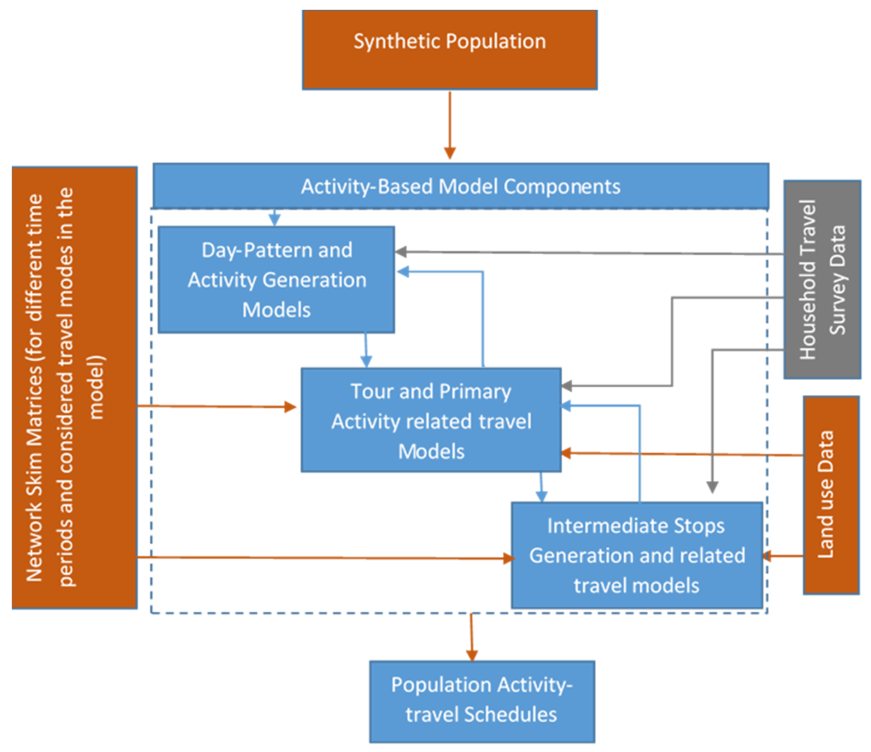
3.1. General Approach

This study follows the methodological framework illustrated in Figure 2. After reviewing previous works, we conducted the data preparation tasks: i.e., extracting the travel time matrices for each mode, land use data of each TAZ, and converting trip-based information in the house travel survey data (HTS) into tour-based information to calibrate the sub-models. The following task is our iterative effort to test different hierarchical structures. This task is described in more detail in Section 3.3. In the end, the selected modeling structure will be validated.

3.2. Data

3.2.1. Study Area

Ho Chi Minh City (HCMC) is the financial and economic center of Vietnam, with a population of 9 million people (HCMC Census 2019). According to the statistics of the HCMC Department of Transport in 2017, about 35% of the road networks have a width of less than 7 m and only 14% are wider than 12 m. Meanwhile, there were approximately 356,429 cars and 6,071,701 motorcycles in use in 2019. However, the public transport system, which is mainly based on buses with 136 routes and 2603 vehicles (in 2017), only counts for less than 10% of total trips. The total area for the bus terminal system, bus stops, and parking lots was only 0.39 square kilometers. The rate of land for transport only accounts for 8.8% of the urban construction land [39].

The growth rate of income per capita of the city was estimated to be six times larger than the growth of the road length [39]. According to the METROS report, the trips were more frequently generated and/or attracted from/to the TAZs of the center business districts (CBDs) and the newly developed districts which are located in the northeast of the city.

Due to this inadequate infrastructure system, the most popular transport mode in HCMC and other cities in Vietnam is the motorcycle, owing to its affordable price, flexible use, and inexpensive parking space.

3.2.2. Household Travel Survey Data

The data were obtained from a large-scale HTS (METROS) conducted in HCMC in 2014 under a project funded by the Japan International Cooperation Agency (JICA). The collected information included household attributes, personal attributes, and one-day travel patterns. The design of the METROS sample was based on the census of HCMC with approximately 1% of total households (nearly 47,000 individuals of 15,000 households).

Table 1. Sociodemographic information.

	Sample Size/Population	Age
		<18	18–25	26–35	36–55	56–65	66–75	>75
METROS (2013)	46,999	13.40%	14.32%	21.90%	37.21%	9.62%	2.53%	1.03%
HCMC (2009)	7,162,864	26.05%	17.89%	20.26%	26.74%	4.58%	2.71%	1.77%
		Education
		Primary school	Secondary school	High school	Vocational	College/University	Post Graduate	None
METROS (2013)		9.54%	25.19%	35.05%	3.99%	21.39%	1.84%	3.01%
HCMC (2009)		19.47%	35.90%	28.80%	3.28%	11.90%	0.51%	0.14%
	Gender (Female)	Number of Household Members
		1	2	3	4	5	6	7+
METROS (2013)	45.94%	0.80%	10.42%	38.12%	36.40%	9.80%	2.89%	1.56%
HCMC (2009)	52.03%	7.42%	16.01%	21.91%	25.40%	12.69%	8.26%	8.30%

presents some sociodemographic statistics of the METROS and this census. The sample distribution was slightly different from the population (p-value of 0.22 to 0.23 in the Chi-square test) because the main target of the survey was to collect the travel patterns of individuals older than six years of age, children less than six years old were assumed to not generate an independent trip. Therefore, the percentage of the population less than 18 years old in the HCMC census was double that in METROS.

There were 3303 households with 26,767 one-day activity schedules remaining after data cleaning. From these schedules, 66,158 home-based tours were obtained, with 36,589 HBO tours accounting for more than 55% of all home-based tours. Figure 3 illustrates the number of tours by primary activity and tour type as either interzone or intrazone. The proportion of intrazonal tours was larger than 52%, except for company business (38.5%).

The HBO tour data set was split into two subsets where 80% of the data were used in the training phase, and the other 20% were used in the validation phase.

3.2.3. Level of Service Data

Using the origin-destination matrix represented in TAZ centroids, car travel time, public bus travel time, and shortest distance were calculated by integrating the GraphHopper Routing Engine (https://www.graphhopper.com/, accessed on 1 November 2019) with the road network from OpenStreetMap (OSM). Travel times by motorbike, walking, and bicycle were derived by the shortest distance and average speeds obtained from the Special Assistance for Project Implementation (SAPI) for HCMC Urban Mass Rapid Transit Line 1, which was conducted in 2013. The survey measured the average speeds of three main transportation modes (car, public bus, and motorcycle) at three time periods: (1) morning peak (6:00 to 9:00), (2) low peak (11:00 to 15:00), and evening peak (16:00 to 19:00). We also assumed that, except for those peak durations, all modes travel at the posted speed limits.

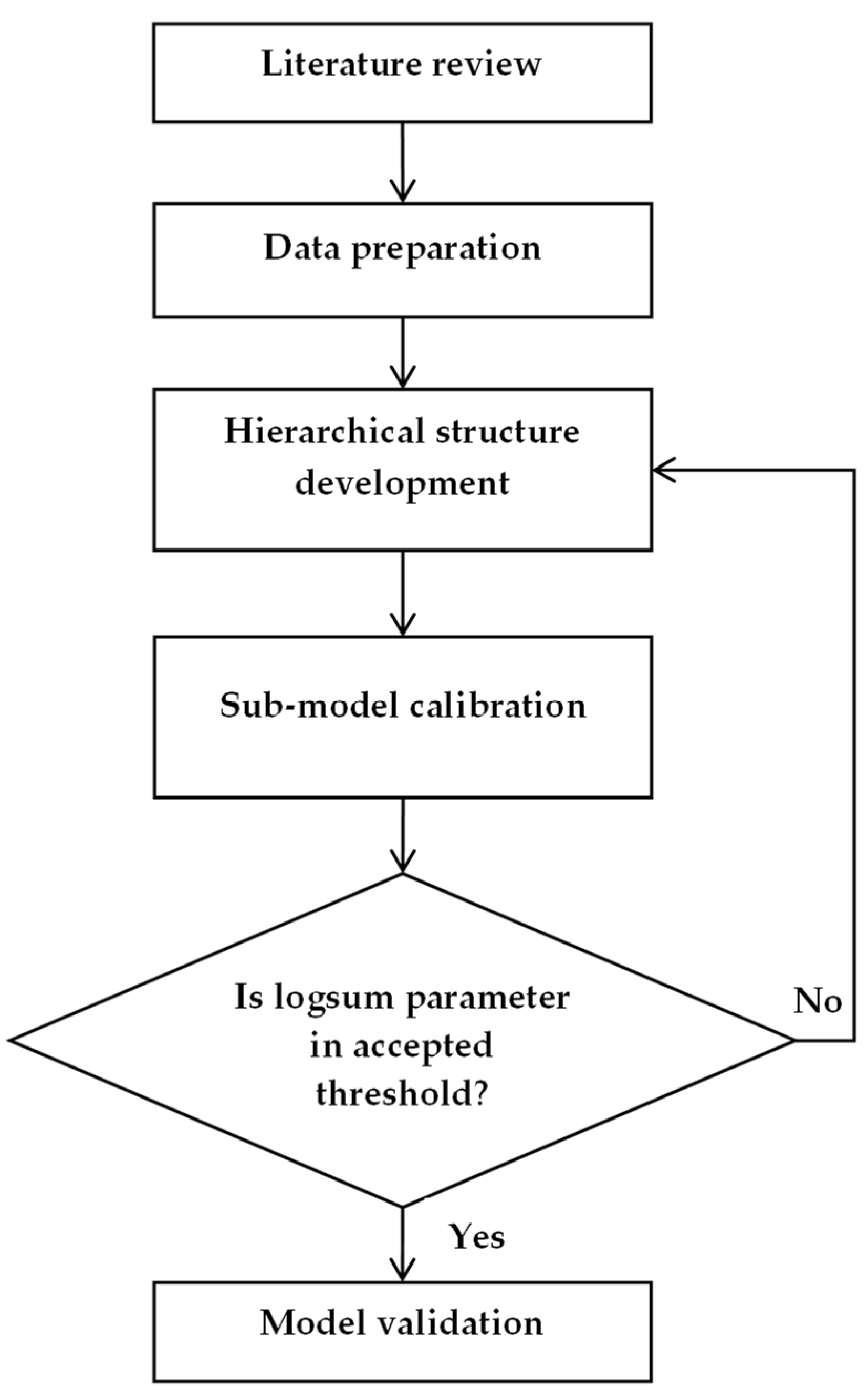
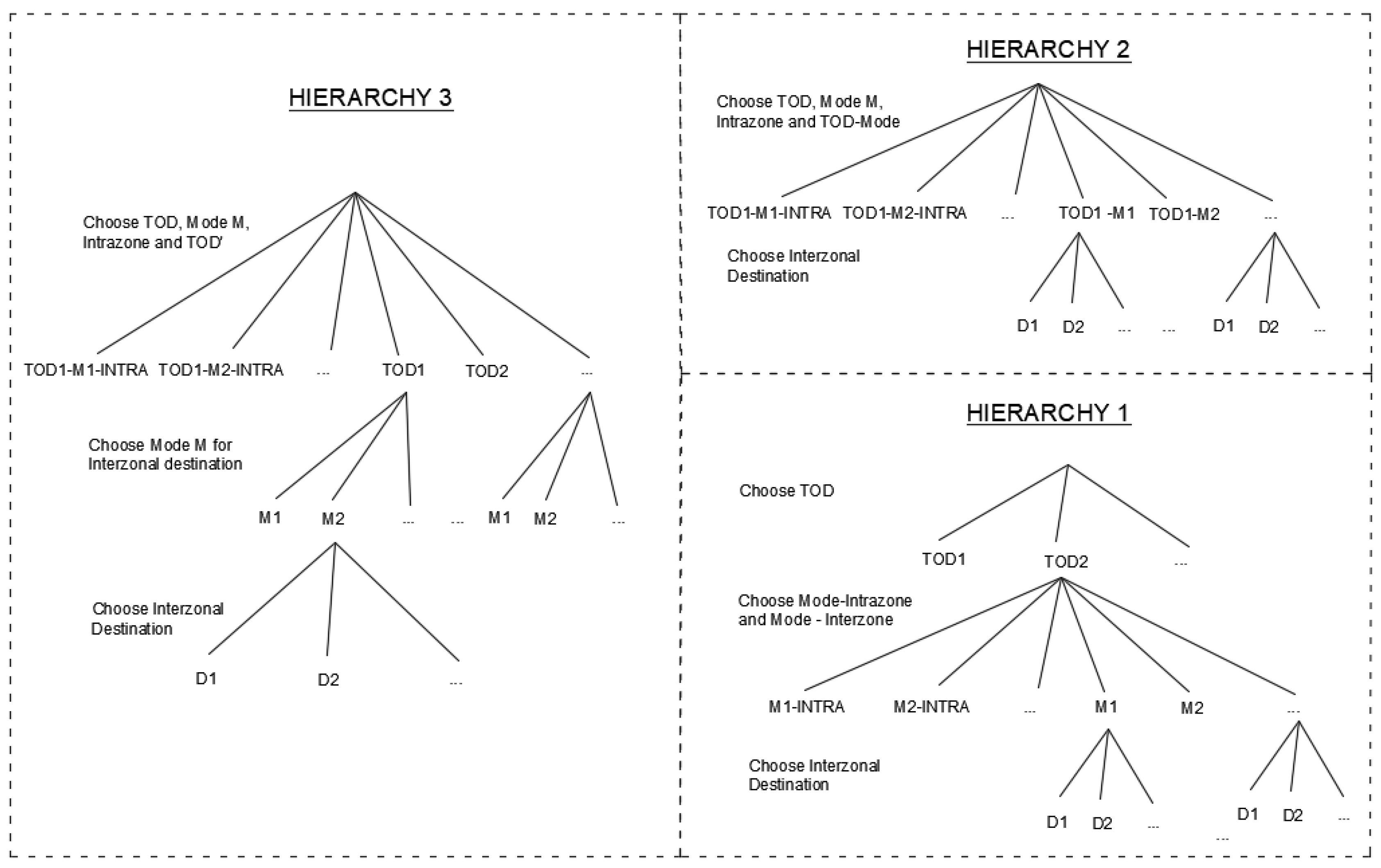
3.3. Hierarchical Structure Development Method

To serve the objectives of this study, a hierarchical structure of ToD, travel mode, and destination choices at the tour level was developed using the large-scale HTS dataset. As activities are different in nature, their scheduling is also different [40]. Therefore, only non-work activities were considered. A similar investigation of work activity scheduling will be conducted in another study.

The hierarchical order of ToD, mode, and destination choice models were constructed step-by-step. First, each choice model was estimated as the bottom model. As the bottom model is constrained by the choice in the upper model, its specification contains the common variables associated with all choice dimensions [41], such as travel time or cost by a certain mode and ToD in our case. The upper models contain the inclusive or logsum values, which carry information from the lower level. Based on the result of the first step, other choice dimensions were added, and the hierarchical order of the two-dimensional choice was tested. Finally, the structures of the three choices were evaluated. The choice models and their interdependences are modeled by MNL and NL models which are popular in many operational ABMs.

Testing for the proper hierarchical structure is based on the informal test of the sign and magnitude of the estimated logsum parameter which connects the lower level to the upper level [12,13,32]. The estimated logsum parameter should fall between zero and one [42]. A judgment can be made on the sensitivity of the level of service variables in the lower-tier model [6].

To investigate the impact of modeling intrazonal tours on structure development, two types of destination choice models were developed: (1) a model with the full destination choice set and (2) a model with the home zone excluded from the destination choice set. In the latter approach, the choice of the home zone is jointly modeled with transport mode and ToD. The impact of the intrazonal tour was represented by a single parameter (β_Intrazone).

The development of structure and models in this study was based on the following assumptions/definitions:

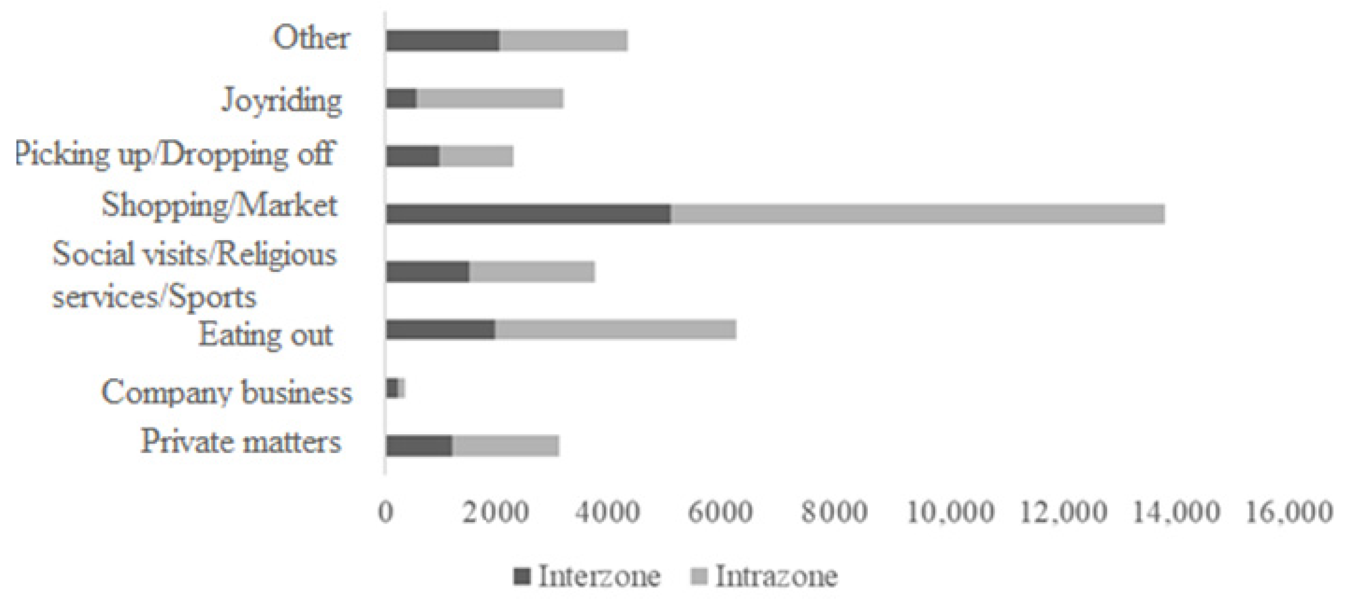
• The activity of the longest duration in the tour was assumed to be the primary activity. All tour choice dimensions were those associated with this primary activity. The concerned activities are (1) private matters (e.g., visit the doctor, go to the bank) (PM), (2) company business (i.e., a work-related activity not at the usual work location) (CB), (3) eating out (EO), (4) social visits/religious services/sports (SRS), (5) shopping/market (SHM), (6) picking up/dropping off (i.e., picking up or dropping off someone or something) (PD), (7) Joyriding (i.e., going out for pleasure normally within the same neighborhood, exercising) (JR), and (8) other activities (OT);
• At the tour level of modeling the HBO tours, all HBW tours were already scheduled. The primary activity and duration were also given;
• The ToD choice set was defined by seven discretized periods based on the observed activity starting time in the data set as follows: (1) ToD1: from 00:00 to 06:30, (2) ToD2: from 06:31 to 08:59, (3) ToD3: from 09:00 to 10:59, (4) ToD4: from 11:00 to 13:59, (5) ToD5: from 14:00 to 15:59, (6) ToD6: from 16:00 to 18:59, and (7) ToD7: from 19:00 to 24:00;
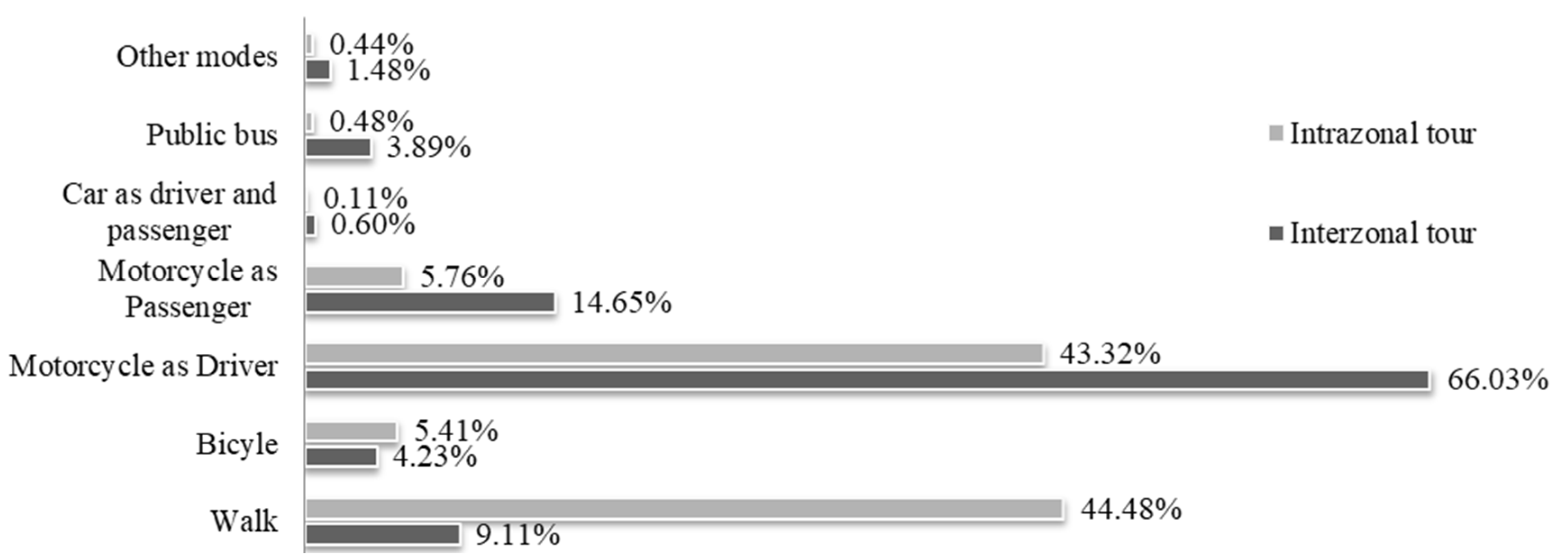
• Tour mode refers to the main transport mode that accounted for the longest distance in the trip chain to the primary activity location. Representative transport modes (Figure 4) were grouped from 24 types in HTS. Other modes were removed due to the unavailable level of service information. The final choice set for transport mode comprised six alternatives: (1) Walking (WK), (2) Bicycle (BI), (3) Motorcycle as a driver (MC_D), (4) Motorcycle as a passenger (MC_P), (5) Car as a driver and a passenger (CAR), and (6) Public bus (PB).

4. Empirical Findings

4.1. Structure Development and the Impacts of Intrazonal Tours

During the effort to develop the hierarchical structures, the travel-time parameter in the ToD choice model was positive when modeled at the bottom level. This result showed that the ToD model was insensitive to the change in the level of service (LOS), which was similar to the observation in [3] that ToD with a broad range should be modeled at the top level.

The order of mode and destination were examined with the consideration of the intrazonal tour as mentioned in Section 3.3. Two hierarchical structures were tested. The first was the structure with the mode conditional on the destination choice. The second was the reversed structure. With the first structure, the range of estimated values for the transport mode logsum parameter ranged from 2.13 to 6.77 under different settings of the choice models and activity types. These results suggested that this hierarchy was inconsistent with the statistical criterion of the nested models [42]. This also reflected the situation in HCMC, where individuals are highly dependent on private transport modes, especially motorcycles. Motorcycles can flexibly maneuver in crowded and small streets, are easier to find parking for, and can carry goods or a pillion rider. Therefore, individuals in HCMC are dependent on this mode of transport for most activities and are more likely to change their destination rather than change their travel mode for all non-work activities.

For the reversed structure, two destination choice models were developed: (1) a model with the full destination choice set and (2) a model with the home zone excluded from the destination choice set. The estimated values of β_Intrazone ranged from 3.0 to 7.0 in the model with the full destination choice set. The estimated travel time parameters ranged from −0.075 to −0.008. However, despite being expected to be positive, the estimated value of the destination logsum parameter in the mode choice models was negative. Theoretically, the logsum represents the inclusive accessibility of all alternatives from the nested model [7]. If this inclusive accessibility value increases, then the utility of the alternative in the upper level associated with that nest would also increase. In this hierarchy, however, the inclusive value only represents the attractiveness of the intrazonal destination and contains almost no accessibility information from other destination alternatives due to the high intrazonal tour proportion in the observed data. Therefore, the hierarchy with intrazones included in the destination choice set was rejected. Meanwhile, in the models that excluded home zones from the choice set, the estimated destination logsum value in the mode choice model was positive and less than one. This structure assumes that destination alternatives conditional on the same mode were assumed to be correlated.

Based on this result, three hierarchical structures (Figure 5) were generated when incorporating ToD with mode and destination choice models. HIERARCHY1 was estimated with the assumption that the joint model of mode—interzone and mode—intrazone is nested in ToD. However, due to the inclusion of intrazone elements, the logsum value from the mode-destination model was negative in the ToD model.

HIERARCHY2 is a two-level nested structure. ToD, mode, and intrazonal destination choices were modeled at the same level and followed by an interzonal destination choice model. The estimated logsum parameter of interzonal destinations was positive but close to zero, which meant that all destinations in the choice set are highly correlated under a given combination of ToD and mode. This result led to the “elimination by aspects” by Tversky [43]. This theory views choice as the probabilistic process in which an individual excludes alternatives from the choice set step-by-step based on certain attributes until only one alternative remains. This model has not been applied in practical ABMs due to its complexity.

The underlying assumption for HIERARCHY3 was that the unobserved attributes of choosing a mode and interzonal destination are correlated conditional on ToD choice. For example, a nonworker in a household can just use the motorcycle before or after the HBW tour of the workers. The logsum parameter in this structure fell in the range from zero to one. HIERARCHY3 was more likely to fit with our data set. This structure is composed of three levels. The top-level (Top model) models the choice of ToD for interzone and ToD and mode of intrazone. The middle level is the mode choice model (MODE). The bottom level is the interzonal destination choice model (DEST). Details of model specifications, estimation, and validation results of the models for different activity types are presented in Section 4.2.

Our results implied the significant effect of intrazonal tours on the development of joint-choice models. The intrazonal tours should be explicitly considered for cases where the data spatial resolution is coarse or the proportion of interzonal tours is high. The choice of intrazone alternative should be made together with other choices [38], meaning that the choice of intrazone should be simultaneously modeled with transport mode and ToD choices in our case.

4.2. Activity Scheduling Models

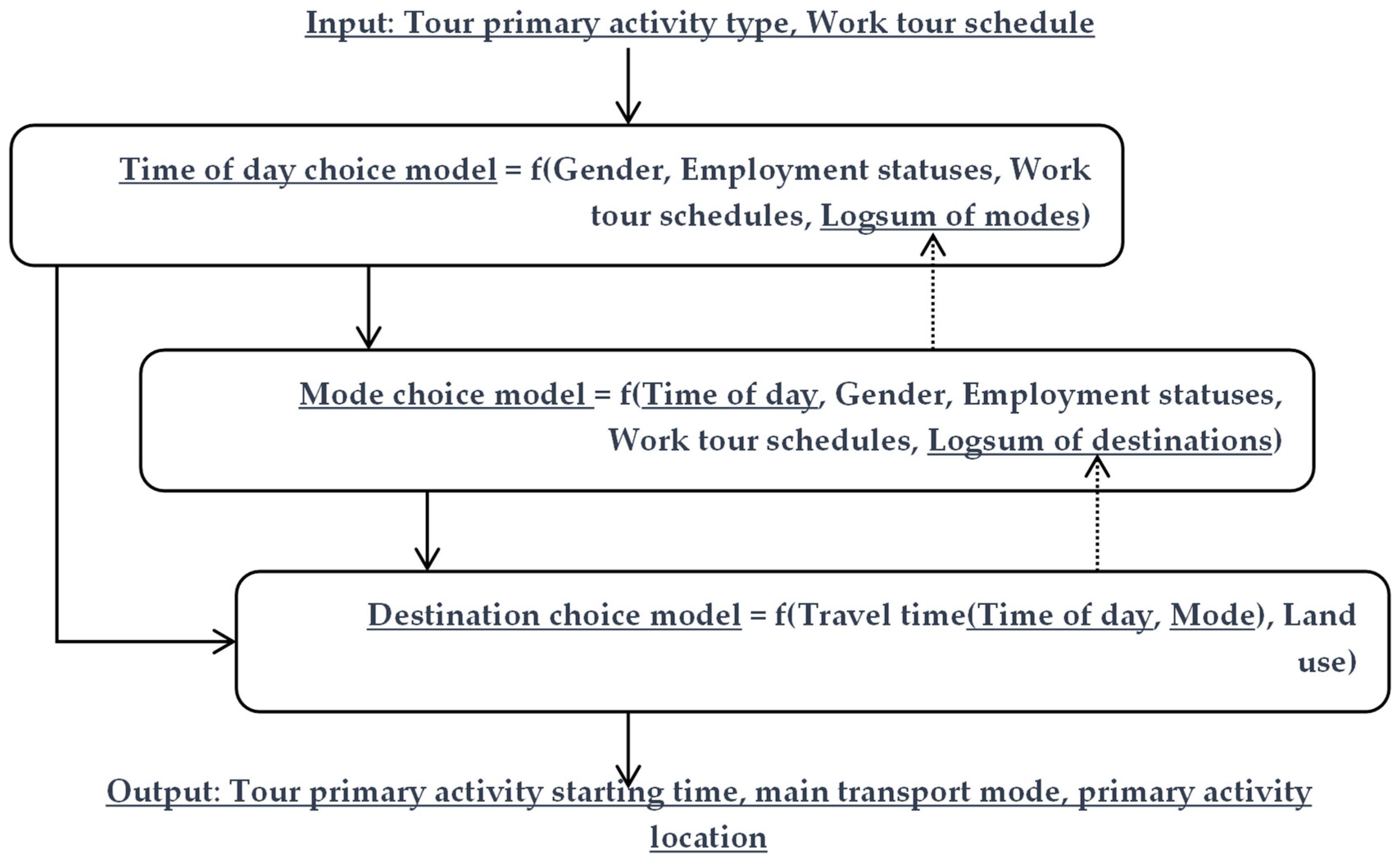
4.2.1. Modeling Framework and Sub-Model Specifications

Each sub-model in HIERARCHY3 is a function of interested variables. As illustrated by the continuous arrows in Figure 6, in our proposed hierarchical structure, the output of the choice in the upper-level model is passed to the models in the lower-level models in the form of explanatory variables. In the other direction, the dash arrows indicate the upward integration of the lower-level models to the upper-level models in the form of logsum values.

The top model is an NL model at an individual’s HBO tour unit. The overall choice set comprised 49 alternatives. Eight models, each corresponding to one type of activity, were estimated. These models are explained by socioeconomic variables such as gender, age, income, vehicle ownership, and daily activity scheduling characteristics such as total work duration and total non-work duration. Employment statuses, either working part-time (work or school duration of less than 4 h) or working full-time (work or school duration of more than 4 h) were defined by the total work duration in the schedule. The duration of employment status and primary activity were used as explanatory variables for the ToD models. To avoid identification issues, a dummy variable for working full-time and an activity duration variable were used in the ToD utility component for alternatives containing interzonal destination choice. Dummy variables for working part-time were used in the ToD utility component for alternatives associated with the intrazonal destination.

The total utility component (V_TMD) of the joint ToD, mode, and destination is written in Equation (1) which is composed of three components: (1) V_{T_Interzone}: the utility component for choosing a ToD with an interzonal destination given in Equation (2), (2) V_T-Intrazone: as the utility component of choosing a ToD with an intrazonal destination given in Equation (3), and (3) V_M-Intrazone: the utility component of choosing mode (M) with an intrazonal destination given in Equation (4).

$$\begin{gathered} {\mathrm{V}}_{\mathrm{TMD}}={\mathrm{ASC}}_{\mathrm{ToD}}+{{\displaystyle \sum }}_{\begin{array}{c}\mathrm{T}\in \mathrm{T}\mathrm{o}\mathrm{D}\\ \mathrm{M}\in \mathrm{M}\mathrm{O}\mathrm{D}\mathrm{E} \end{array}}\left[{\mathrm{V}}_{\mathrm{T}-\mathrm{Intrazone}}+{\mathrm{V}}_{\mathrm{M}-\mathrm{Intrazone}}+{\mathsf{\beta }}_{\mathrm{Intrazone}}\right]{\ast \mathrm{X}}_{\mathrm{Intrazone}}+ \\ {{\displaystyle \sum }}_{\mathrm{T}\in \mathrm{ToD}}\left[{\mathrm{V}}_{\mathrm{T}-\mathrm{Interzone}}+{\mathsf{\beta }}_{{\mathrm{logsum}}_{\mathrm{MODE}}}{\ast \mathrm{logsum}}_{\mathrm{MODE}}\right]\ast \left(1-{\mathrm{X}}_{\mathrm{Intrazone}}\right), \end{gathered}$$

(1)

$${\mathrm{V}}_{\mathrm{T}-\mathrm{Interzone}}={{\displaystyle \sum }}^{\hspace{0.17em}}{\mathsf{\beta }}_{\mathrm{Ti}\_\mathrm{Interzone}}{\ast \mathrm{X}}_{\mathrm{T}}{\ast \mathrm{TOD}}_{\mathrm{i}},$$

(2)

$${\mathrm{V}}_{\mathrm{T}-\mathrm{Intrazone}}={{\displaystyle \sum }}^{\hspace{0.17em}}{\mathsf{\beta }}_{\mathrm{Ti}\_\mathrm{Intrazone}}{\ast \mathrm{X}}_{\mathrm{T}}{\ast \mathrm{TOD}}_{\mathrm{i}},$$

(3)

$${\mathrm{V}}_{\mathrm{M}-\mathrm{Intrazone}}={\mathrm{ASC}}_{\mathrm{MODE}\_\mathrm{Intrazone}}+{{\displaystyle \sum }}^{\hspace{0.17em}}{\mathsf{\beta }}_{\mathrm{Mj}\_\mathrm{Intrazone}}{\ast \mathrm{X}}_{\mathrm{M}}{\ast \mathrm{MODE}}_{\mathrm{j}},$$

(4)

where:

• ASC_TOD: alternative specific constant for each ToD alternative;
• ASC_{MODE_Intrazone}: transport mode alternative specific constant associated with the choice of transport mode to the intrazonal destination;
• β_{Ti_Interzone}: specific parameters associated with ToD_i and interzonal destination;
• β_{Ti_Intrazone}: specific parameters associated with ToD_i and intrazonal destination;
• β_Intrazone: specific parameter for alternatives associated with intrazonal destination;
• β_logsumMODE: log sum parameter from interzonal mode choice model;
• β_{Mj_Intrazone}: specific parameters associated with transport mode j and intrazonal destination;
• X_M, X_T: explanatory variables;
• Dummy ${\mathrm{TOD}}_{\mathrm{i}}=\{\begin{array}{c}1 {\mathrm{if}\mathrm{alternative}\mathrm{containing}\mathrm{TOD}}_{\mathrm{i}}\\ 0 \mathrm{otherwise}\end{array}$;
• Dummy ${\mathrm{MODE}}_{\mathrm{j}}=\{\begin{array}{c}1 \mathrm{if}\mathrm{alternative}\mathrm{containing}\mathrm{transport}\mathrm{mode}\mathrm{j}\\ 0 \mathrm{otherwise}\end{array}$;
• Dummy ${\mathrm{X}}_{\mathrm{Intrazone}}=\{\begin{array}{c}1 \mathrm{if}\mathrm{alternative}\mathrm{containing}\mathrm{intrazonal}\mathrm{destination}\\ 0 \mathrm{otherwise}\end{array}$;
• logsum_MODE: The logsum term from the nesting mode choice model for alternatives associated with interzonal destinations.

The utility function of the MODE model was formulated as in Equation (5) as follows:

$${\mathrm{V}}_{\mathrm{MODE}}={\mathrm{ASC}}_{\mathrm{MODE}}+{{\displaystyle \sum }}^{\hspace{0.17em}}{\mathsf{\beta }}_{\mathrm{z}}\ast \mathrm{Z}+{{\displaystyle \sum }}^{\hspace{0.17em}}{\mathsf{\beta }}_{\mathrm{ToD}}\ast \mathrm{ToD}+{\mathsf{\beta }}_{\mathrm{logsumDEST}}{\ast \mathrm{logsum}}_{\mathrm{DEST}}$$

(5)

where:

• ASC_MODE: transport mode alternative specific constant that is used to capture the unobserved attributes in the choice of transport mode to the interzonal destination;
• β_logsumDEST: log sum parameter from interzonal destination choice model;
• Z: explanatory variables including household/personal attributes such as vehicle ownership, age, gender, and income;
• ToD: dummy variable for time-of-day periods;
• logsum_DEST: The log sum term from the interzonal destination model.

In the DEST model, the choice set was sampled using an average ratio value between activity duration and travel time described in [18]. This approach was based on the assumption elaborated by Dijst and Vidakovic [44] that individuals are willing to spend a long travel time on activities of a long duration and vice versa. Population (pop) and surface area (area) were the size variables. In the construction of the data, due to the lack of travel cost information as part of the data accuracy issues in developing countries [19], the effort to include travel costs in the model was not successful. Therefore, only travel time as a generic variable (tt_TOD-MODE) was considered. ${\mathsf{\beta }}_{\log }$ was introduced to capture the sensitivity of the model to the zoning system [45]. The utility function of choosing a destination outside the home zone is presented in Equation (6).

$${\mathrm{V}}_{\mathrm{DEST}}={\mathsf{\beta }}_{\mathrm{travel}\_\mathrm{time}}{\ast \mathrm{tt}}_{\mathrm{ToD}-\mathrm{MODE}}+{\mathsf{\beta }}_{\log }\ast \log \left(\exp \left({\mathsf{\beta }}_{\mathrm{pop}}\right){\ast \mathrm{pop}}_{\mathrm{DEST}}+{\mathrm{area}}_{\mathrm{DEST}}\right)$$

(6)

These two models were calibrated with the pooled data of all activities due to a lack of land use data related to different activity types.

4.2.2. Modeling Results and Discussions

PythonBiogeme, an open-source package for discrete choice models [46], was adopted for the model estimations. Summaries of the results are presented in

Table 2. Top models.

Parameters	Alternative	PM	CB	EO	SRS	SHM	PD	JR	OT
ToD alternative-specific variable	ToD1	0.52 (2.95) **		−2.19 (−10.81) ***	−1.74 (−7.11) ***	−0.23 (−3.03) **	0.26 (1.32)	−0.21 (−1.18)	−1.32 (−7.83) ***
	ToD2	0.71 (4.53) ***	2.24 (5.44) ***	−0.50 (−4.21) ***	−1.07 (−6.55) ***	1.44 (24.23) ***	2.41 (14.42) ***	−0.82 (−3.26) **	0.37 (3.40) ***
	ToD3	−0.07 (−0.39)	2.51 (6.23) ***	−1.90 (−16.87) ***	−2.52 (−10.17) ***	0.29 (3.91) ***	0.41 (2.16) **	−3.08 (−15.40) ***	−0.43 (−4.52) ***
	ToD4	−1.09 (−4.77) ***	1.78 (4.29) ***	−2.74 (−12.19) ***	−2.59 (−15.09) ***	−1.39 (−11.90) ***	1.36 (8.11) ***	−3.39 (−5.33) ***	−0.88 (−6.14) ***
	ToD5	0.73 (4.25) ***	1.72 (4.11) ***	−2.48 (−10.92) ***	−1.17 (−7.07) ***	0.05 (0.64)	−0.14 (−0.57)	−1.77 (−7.73) ***	0.27 (2.67) **
	ToD6	0.88 (5.67) ***	2.28 (5.40) ***	−0.86 (−15.42) ***	−0.24 (−3.41) ***	0.64 (10.09) ***	1.85 (11.43) ***	−0.19 (−2.49) **	−0.06 −(0.82)
	ToD7	0 (constrained)
Choosing ToD: Interzonal destination component
Parameters		PM	CB	EO	SRS	SHM	PD	JR	OT
Primary activity duration	ToD1-Interzone	0.37 (2.75) **		0.96 (6.77) ***	0.79 (4.61) ***			0.75 (4.64) ***	0.37 (5.56) ***
	ToD2-Interzone	0.79 (9.03) ***	0.36 (4.36) ***	0.94 (10.79) ***	1.19 (11.79) ***			0.69 (3.04) **	0.39 (9.84) ***
	ToD3-Interzone	0.79 (7.95) ***	0.22 (2.48) **	1.02 (9.45) ***	1.35 (11.44) ***			1.03 (4.19) ***	0.35 (7.40) ***
	ToD4-Interzone	0.93 (8.54) ***		1.38 (14.98) ***				1.13 (4.45) ***	0.38 (6.65) ***
	ToD5-Interzone	0.34 (2.60) **		1.06 (8.24) ***				0.99 (5.57) ***
	ToD6-Interzone	0.37 (3.36) ***	−0.41 (−1.68) *	1.15 (16.09) ***	0.83 (8.92) ***			0.84 (5.86) ***
	ToD7-Interzone			0.73 (10.47) ***	0.41 (4.19) ***			0.84 (6.46) ***	−0.25 (−2.89) **
Dummy: Total duration of work activity in schedule more than 4 h	ToD1-Interzone	−2.77 (−8.68) ***		−2.35 (−4.93) ***	−3.50 (−4.80) ***		−1.15 (−2.19) **	−2.41 (−4.05) ***	−2.62 (−5.05) ***
	ToD2-Interzone	−3.89 (−8.36) ***		−2.88 (−9.48) ***	−2.51 (−7.54) ***		−0.74 (−3.33) ***	−2.62 (−2.57) **	−2.86 (−9.50) ***
	ToD3-Interzone	−1.30 (−1.75) *							−1.31 (−1.80) *
	ToD4-Interzone	−1.47 (−2.75) **		0.67 (2.08) **			−2.26 (−2.23) **
	ToD5-Interzone	−0.70 (−2.86) **		0.77 (2.25) **			0.92 (1.82) *	1.30 (2.38) **
	ToD6-Interzone	−0.37 (−2.46) **			−0.65 (−4.42) ***
	ToD7-Interzone		1.63 (2.71) **	0.45 (5.52) ***	0.30 (2.29) **	1.88 (22.90) ***	1.23 (5.01) ***	1.09 (7.98) ***	0.54 (4.90) ***
Logsum from MODE (βlogsumMODE)	All ToD alternatives	0.63 (10.63) ***	1.05 (5.11) ***	0.49 (11.46) ***	0.77 (12.97) ***	0.88 (25.90) ***	1.00 (11.51) ***	0.41 (5.66) ***	0.70 (13.85) ***
Choosing ToD-MODE: Intrazonal destination component
Parameters		PM	CB	EO	SRS	SHM	PD	JR	OT
Total duration of nonwork activities in schedule	ToD1-Intrazone	2.83 (14.03) ***	2.56 (5.07) ***	1.82 (14.88) ***	2.44 (9.54) ***	0.53 (5.58) ***	0.52 (2.78) **	1.56 (9.62) ***	1.68 (8.10) ***
	ToD2-Intrazone	3.27 (9.22) ***	1.78 (5.64) ***	2.24 (22.35) ***	2.81 (10.68) ***	1.38 (13.89) ***	0.60 (3.74) ***	2.14 (4.63) ***	1.75 (9.87) ***
	ToD3-Intrazone	0.50 (1.60)			0.81 (2.66) **	−0.48 (−3.26) **
	ToD4-Intrazone	0.23 (1.10)				−1.26 (−7.28) ***
	ToD5-Intrazone	0.27 (2.10) **				−1.88 (−16.90) ***	−0.63 (−1.81) *	−1.04 (−3.65) ***	−0.37 (−2.42) **
	ToD6-Intrazone				0.43 (3.41) ***	−1.25 (−15.83) ***	-	-	-
	ToD7-Intrazone			−0.66 (−7.16) ***	−0.34 (−2.52) **	−2.09 (−21.53) ***	−1.22 (−3.41) ***	−0.63 (−6.30) ***	−0.60 (−5.16) ***
Dummy: Total duration of work activity in schedule of less than 4 h	ToD1-Intrazone	−1.19 (−4.37) ***		0.26 (1.28)	−1.22 (−3.80) ***	−0.31 (−3.22) **	- -	−1.53 (−6.77) ***	−0.65 (−2.74) **
	ToD2-Intrazone	−2.59 (−6.73) ***		−0.78 (−5.71) ***	−1.86 (−6.60) ***	−1.83 (−18.44) ***	−0.70 (−4.30) ***	−3.00 (−5.87) ***	−1.75 (−9.33) ***
	ToD3-Intrazone	−0.18 (−0.74)				−0.36 (−2.62) **
	ToD4-Intrazone	0.46 (2.49) **		0.35 (1.53)					−0.55 (−3.24) **
	ToD5-Intrazone	0.70 (3.65) ***		0.36 (1.64) *	0.24 (1.43)				−0.34 (−2.49) **
	ToD7-Intrazone		0.77 (1.55)			0.39 (5.45) ***
Number of activities in tours	MC_D-Intrazone	0.11 (0.83)		0.41 (4.44) ***	0.11 (0.84)	0.37 (6.32) ***	0.21 (1.44)	0.61 (2.03) **	0.16 (1.78) *
	PB-Intrazone				0.71 (1.30)
Dummy: Personal income not reported	MC_D-Intrazone	−1.24 (−10.58) ***		−1.24 (−14.40) ***	−0.89 (−6.32) ***	−0.62 (−9.01) ***	−0.22 (−1.32)	−1.04 (−3.73) ***	−0.87 (−9.01) ***
	MC_P-Intrazone	0.61 (1.94) *		−0.31 (−1.52)	−0.68 (−2.24) **	−0.02 (−0.10)	−0.92 (−2.24) **		−1.00 (−3.54) ***
	PB-Intrazone			-	−1.15 (−1.55)
Personal income	MC_P-Intrazone			−0.14 (−4.24) ***	−0.26 (−3.75) ***	0.00 (0.02)	−0.61 (−4.02) ***		−0.31 (−4.79) ***
	PB-Intrazone				−0.44 (−1.76) *
	MC_D-Intrazone				0.06 (3.33) ***	0.08 (8.80) ***	0.15 (6.48) ***	0.06 (2.26) **
Number of MC/HH workers	MC_P-Intrazone	0.39 (4.57) ***		0.42 (7.69) ***	0.58 (7.78) ***	0.74 (20.31) ***	0.57 (5.85) ***		0.49 (6.78) ***
Dummy: Person age <18	BI-Intrazone	2.46 (9.13) ***		2.53 (10.06) ***	2.00 (9.89) ***	0.74 (4.85) ***	−1.04 (−2.11)	2.73 (7.24) ***	1.75 (8.60) ***
Dummy: Person age >65	WK-Intrazone	1.25 (7.93) ***		1.22 (8.18) ***	1.17 (7.31) ***	0.97 (9.28) ***	2.16 (5.55) ***	0.85 (4.83) ***	0.95 (6.83) ***
Personal income	PB-Intrazone				1.69 (2.40) **				1.54 (1.91) *
Female	PB-Intrazone				0.65 (1.18)
Dummy: Student	PB-Intrazone				1.36 (1.94) *
Mode specific variable	BI-Intrazone	−2.84 (−10.77) ***	−2.50 (−4.84) ***	−2.99 (−14.38) ***	−2.24 (−9.00) ***	−0.68 (−6.64) ***	−1.64 (−5.76) ***	−1.74 (−3.59) ***	−1.96 (−10.83) ***
	MC_P-Intrazone	−2.42 (−7.61) ***	−3.11 (−4.32) ***	−0.66 (−2.99) **	−0.78 (−2.37) **	−0.92 (−4.86) ***	−0.35 (−0.80)	−0.96 (−2.15) **	−0.34 (−1.17)
	WK-Intrazone	0.29 (1.50)	−0.86 (−3.75) ***	0.26 (2.01) **	0.27 (1.36)	0.94 (9.93) ***	−1.48 (−5.75) ***	3.07 (7.91) ***	0.20 (1.39)
	PB-Intrazone				−3.12 (−3.09) **	−2.74 (−13.16) ***			−3.53 (−8.77) ***
Intrazone specific variable (βIntrazone)	All alternatives	4.34 (7.86) ***	7.92 (4.39) ***	4.11 (10.70) ***	6.06 (11.93) ***	6.84 (23.89) ***	7.93 (11.31) ***	2.76 (3.80) ***	5.24 (11.84) ***
Sample size		2431	264	4866	2934	10,932	1775	2530	3337
Rho-square-bar		0.20	0.25	0.25	0.24	0.20	0.25	0.36	0.18

Significance code: ***: 1% significance level **: 5% significance level; *: 10% significance level.

,

Table 3. MODE model.

Parameters	Alternative	Value (t-Test in Parentheses)
Alternative specific constants	Bicycle	−2.6	(−8.26) ***
	Car	−1.98	(−3.09) **
	Motorcycle as passenger	−0.938	(−7.61) ***
	Public bus	−2.25	(−4.72) ***
	Walk	−0.811	(−1.73) *
	Motorcycle as driver	-	-
Dummy-TOD1 (from 0:00 to 6:30)-(MC_D as the base case)	Walk	0.861	(4.59) ***
	Bicycle	1.23	(4.43) ***
	Motorcycle as passenger	−0.718	(−5.06) ***
	Public bus	1.42	(3.33) ***
	Car	-	-
Dummy-TOD2 (from 6:31 to 8:59)-(MC_D as the base case)	Walk	0.238	(1.67) *
	Bicycle	0.422	(1.44)
	Motorcycle as passenger	0.134	(0.92)
	Public bus	0.261	(1.13)
	Car	-	-
Dummy-TOD3 (from 9:00 to 10:59)-MC_D as the base case)	Walk	-	-
	Bicycle	0.39	(1.19)
	Motorcycle as passenger	−0.864	(−6.09) ***
	Public bus	2.06	(5.55) ***
	Car	-	-
Dummy-TOD4 (from 11:00 to 13:59)-(MC_D as the base case)	Walk	0.402	(1.34)
	Bicycle	1.51	(5.03) ***
	Motorcycle as passenger	−0.925	(−4.57) ***
	Public bus	2.09	(4.99) ***
	Car	-	-
Dummy-TOD5 (from 14:00 to 15:59)-(MC_D as the base case)	Walk	−0.49	(−1.78) *
	Bicycle	1.22	(4.99) ***
	Motorcycle as passenger	−0.994	(−7.08) ***
	Public bus	2.55	(7.61) ***
	Car	-	-
Dummy-TOD6 (from 16:00 to 18:59)-(MC_D as the base case)	Walk	-	-
	Bicycle	0.845	(3.8) ***
	Motorcycle as passenger	−0.394	(−4.24) ***
	Public bus	1.82	(5.43) ***
	Car	-	-
Person Age <18	Bicycle	1.82	(8.93) ***
	Motorcycle as passenger	1.17	(6.22) ***
Person age >65	Motorcycle as passenger	1.01	(6.7) ***
	Public bus	1.11	(5.15) ***
	Walk	1.17	(5.87) ***
Female	Motorcycle as passenger	1.21	(17.04) ***
	Public bus	0.292	(2.28) **
Personal income not reported (Dummy: 1–Income not reported; 0 otherwise)	Car	−0.628	(−1.13)
	Motorcycle as driver	−0.699	(−5.97) ***
	Motorcycle as passenger	−0.191	(−1.97) **
Personal income	Car	0.156	(6.26) ***
	Motorcycle as driver	0.125	(8.1) ***
Student	Public bus	0.639	(3.00) **
Number of CAR/HH workers	Car	1.76	(2.55) **
Number of MC/HH workers	Motorcycle as driver	0.693	(13.58) ***
Home zone in CBD	Bicycle	0.624	(3.95) ***
	Public bus	0.369	(1.67) *
	Walk	1.15	(4.12) ***
Home zone in NDD	Public bus	0.899	(3.95) ***
Number of activities in tour	Car	0.386	(1.02)
	Public bus	−0.407	(−2.24) **
Dummy for bring/get activity in tour	Car	1.00	(1.71) *
	Motorcycle as driver	0.781	(6.17) ***
	Public bus	−1.2	(−2.8) **
Logsum–destination	All alternatives	0.538	(8.55) ***
Init log likelihood:	−14,299.53
Final log likelihood:	−6188.046
Likelihood ratio test for the init. model:	16,222.969
Rho-square for the init. model:	0.567
Rho-square-bar for the init. model:	0.564

Significance code: ***: 1% significance level **: 5% significance level; *: 10% significance level.

and

Table 4. DEST model.

Parameters	Value	t-Test
$\mathrm{Parameter}\mathrm{of}\mathrm{the}\mathrm{size}\mathrm{part}{\mathsf{\beta }}_{\log }$	0.703	34.95 ***
$\mathrm{Population}{\mathsf{\beta }}_{\mathrm{pop}}$	4.81	0.79
$\mathrm{Area}{\mathsf{\beta }}_{\mathrm{area}}$ (constrained)	0	-
$\mathrm{Travel}\mathrm{time}{\mathsf{\beta }}_{\mathrm{travel}\_\mathrm{time}}$	−0.173	−90.73 ***
Sample size:	9079
Rho-square-bar:	0.142

Significance code: ***: 1% significance level **: 5% significance level; *: 10% significance level.

for the top models, MODE, and DEST models, respectively. Most parameters were estimated with the expected sign and 90% significance level except for some parameters associated with few observed alternatives.

Table 2 summarizes the estimated parameters of the top models for eight activities. The adjusted rho-squared, which ranged from 0.18 to 0.36, is reasonable for a complex joint model. The differences in estimated parameters across the models suggested heterogeneity in the scheduling of different activities. The negative ASC_TOD in the “Eating out”, “Social visits/Religious services/Sports”, and “Joyriding” models indicated that these activities are less likely to start in the daytime when other variables were set to zero. As a part of city culture, residents prefer to go out in the evening for entertainment after a day of work to avoid the high daytime temperatures. Most services in HCMC are open until 10:00 p.m.

Regarding the estimation results in the interzonal components, the structure characterized by the log sum values (β_logsumMODE) from the lower level in most models ranged from 0.41 to 1.05 with good statistical significance. The largest values in the “Picking up/Dropping off” and “Company business” models indicated the independence of transport mode alternatives under a given ToD. As the log sum captures the correlation among tour transport mode alternatives, the log sum parameter attaining a value of one indicated that when scheduling for these activities, choosing ToD is not conditional on the choice of transport mode. The results suggested different scheduling structures for each activity type. The impact of working status and sociodemographic variables also vary by the different activity types. Except for the “Shopping/Market” and “Picking up/Dropping off” models, activity duration significantly impacts the choice of starting time in interzonal tours. The longer the activity duration is, the earlier the time of day that the activity is started. Most of the estimated parameters for daytime ToD alternatives associated with full-time working individuals were negative, which indicated that these individuals are less likely to start non-work or school activities in interzonal destinations during the daytime. Similarly, part-time workers were less likely to schedule these activities in the home zone in the morning.

In the intrazonal components, β_Intrazone parameters captured the unobserved attributes in scheduling the activities in the home zone. The large β_Intrazone is explained by the highly observed proportion of intrazonal tours. The negative intrazone mode parameters in the “Company business” and “Picking up/Dropping off” models meant that the most preferred mode was MC_D (driving a motorcycle) for traveling in the home zone while walking was more preferred for other activity types. The reason might be because these activities are temporally inflexible and individuals may not want to take the risk of being late by choosing a slower mode. These results suggested that the choice of intrazonal destination for non-work activities is constrained by other factors in addition to land use variables such as available transport mode, time, and the individuals’ schedule of work activities.

The MODE model (Table 3) had good performance with an adjusted rho-squared value of 0.564, while that of the DEST was 0.14.

In MODE, the estimated parameters ToD3, ToD4, and ToD5 associated with PB showed that individuals are more likely to choose to travel by public bus for activities started during low congestion periods. Because there is no separate infrastructure for public transport in HCMC, it takes much longer to travel by bus than by motorcycle during peak hours.

Females, university students, and elderly people, who seemed to have more flexible time than their counterparts, had higher utility toward public buses. Secondary or high school students were more likely to choose bicycles. Individuals living in the CBDs and the newly developed districts (NDDs) were more likely to choose public buses, walking, and bicycles than individuals living in rural areas (RAs). Personal income significantly affected the choice of travel mode in interzonal tours. In general, individuals with higher income are more likely to travel by their private mode of transportation.

In addition, choosing a motorcycle was not dependent on tour complexity, which is similar to the descriptive information in [47]. Narrow streets, especially in the CBD, the flexibility of motorcycles, and the congestion of the underdeveloped infrastructure in the city are among the reasons that explain these behaviors.

The negative value of the dummy representing if the tour encompassed a pick up or drop off activity by PB indicated that adding a stop to the tour also decreased the utility of choosing a public bus. This result explained the fact that people do not want to use public buses to perform complex tours due to the low connectivity of the existing bus network to many urban land-use functions, such as schools. The low probability of choosing public buses in the RA is explained by the unequal or underdeveloped bus network among the three areas. As described by Van et al. [48], more than 60% of the distances from the household location to the nearest bus stop in RA are larger than 1 km, while this ratio is less than 10% in the CBD and 35% in NDDs.

In the DEST model (Table 4), the estimated general travel time parameter had a negative sign with a high significance level. The size parameter of 0.703 was also statistically significant. This result indicated that the model is sensitive to the zonal system [45]. The estimated parameters of the population were insignificant, and the area parameter was constrained to one. The reason for this result is that population and area variables are not enough to explain the attractiveness of a zone for non-work or school activities.

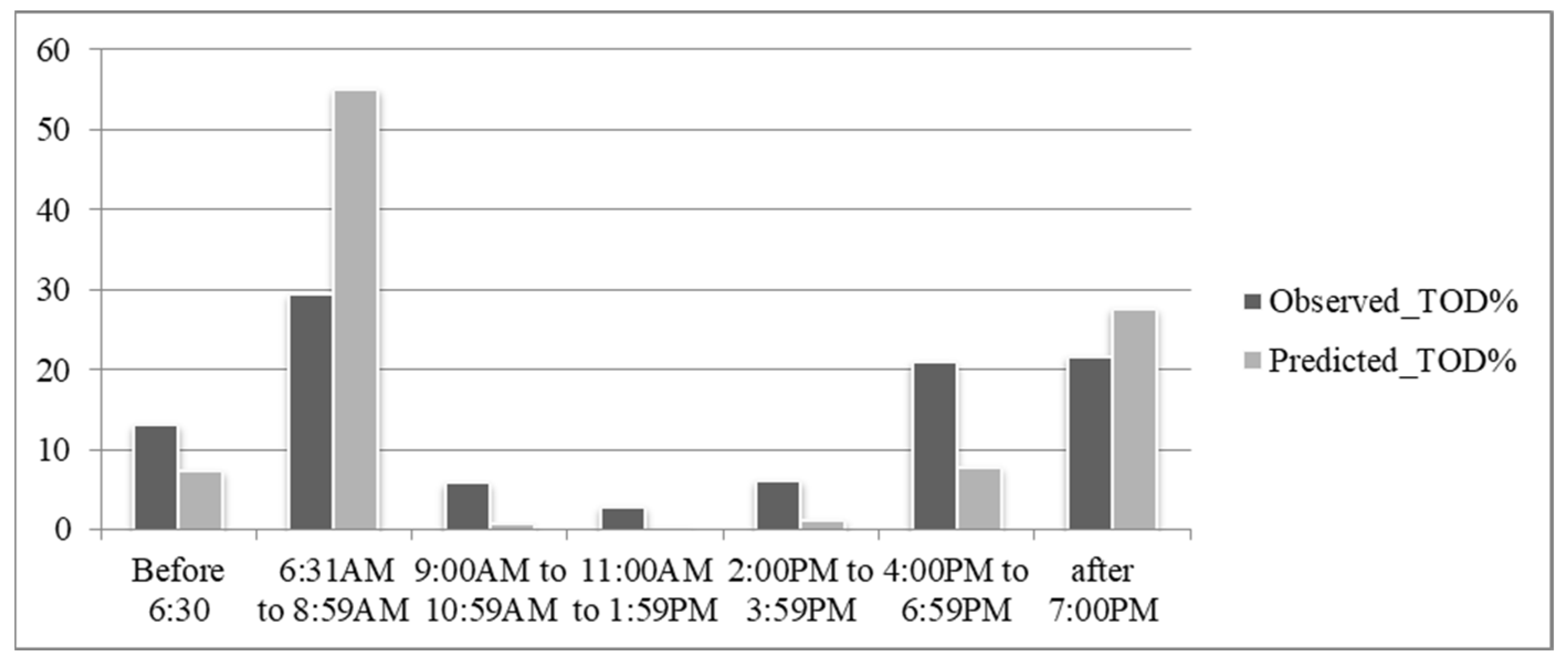
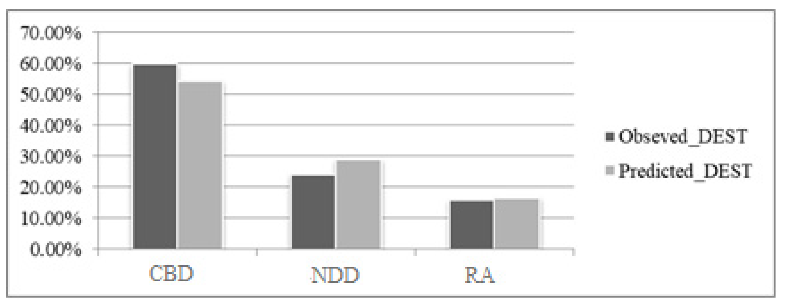
4.2.3. Model Validation

Petrick et al. [49] used various measures to compare the results from different settings of sub-models in an ABM model. Those measures were derived by grouping modeling output as the number of tours, number of trips, number of stops, etc., and then stratifying those aggregate outcomes into different segments. The authors also suggested that the method can be used to test models that have hierarchical structures with sub-models. Drchal et al. [50] proposed a statistical validation framework using the Kolmogorov–Smirnov two-sample (KS) statistic for a better comparison of the output of ABM models.

Our proposed hierarchical structure consisted of three integrated sub-models for choices at the tour level. The output was the predicted starting time, the main transport mode, and the destination of the primary activity for each individual. The aggregate validation measures consisting of frequencies of ToD, mode, and destination choices at aggregate zone levels are presented in Figure 7, Figure 8 and Figure 9.

In the KS test comparing two dataset values, the higher p-value suggests a smaller difference between them. With the KS statistics’ p-values larger than 0.05 for all measures, the proposed model produced similar prediction results to the observations.

At the disaggregated level, the distributions of ToD, mode, and 1 km-interval tour distance (distance from home zone to destination) stratified by activity type, age group, and employment status were used as validation measures. KS statistics were calculated for each case. The results are summarized in

Table 5. Disaggregate results by Age and Employment status and Activities: p-value of Kolmogorov–Smirnov test.

Category	ToD	Mode	Distance
Age
<18	0.96	0.70	0.72
18–25	0.21	0.82	0.36
26–35	0.58	0.69	0.12
36–55	0.58	0.59	0.36
56–65	0.54	0.92	0.38
66–75	0.2	0.96	0.39
>75	0.74	0.68	0.07
Employment status
No work	0.58	0.59	0.39
Part-time	0.74	0.92	0.15
Full-time	0.21	0.93	0.17
Activity type
Private matters	1.00	0.97	0.76
Company business	0.09	0.50	0.42
Eating out	0.31	1.00	0.65
Social visits/Religious services/Sports	0.78	0.80	0.07
Shopping/Market	0.42	1.00	0.89
Picking up/Dropping off	0.85	0.92	0.51
Joyriding	0.33	0.99	0.59
Other	0.42	0.90	0.05

. Tour distance had the poorest performance. The tour distance distributions of “Social visits/Religious services/Sports” and “Other” activities were the most different at a significance level of less than 10%. Destination choice for these activities is quite a challenge since the activities themselves contain multiple purposes that require different spatial settings of opportunities. While their temporal patterns in terms of activity start time and duration may be similar [18], their spatial patterns are not. “Company business” tours were significantly different from the observation regarding the ToD measure but not for the other two measures.

5. Concluding Remarks

In this paper, we successfully developed a hierarchical structure to represent the interdependence among the choices of ToD, mode, and destination choice in the scheduling of non-work or school activities at the tour level of an ABM for MBCs.

The main findings are as follows. First, by separately considering intrazone alternatives, the hierarchy with ToD choice at the top level, transport mode choice in the middle, and destination choice at the bottom level is the most appropriate structure. Similar to the interdependence between the mode and destination choices of car-dominated cities [12], the transport mode is less likely to be switched than the destination in motorcycle-dominated cities such as HCMC, whereas the reversed order is applicable in the Jakarta model [24]. Our result, therefore, contributed to the empirical evidence that there is a correlation between the modal split pattern and the hierarchical structure of mode and destination choices.

Second, our experiment confirmed the significance of modeling intrazonal destination choice on structure development. Intrazonal trips/tours should be modeled in conjunction with other choice dimensions, such as travel mode and time choice.

Third, the variation in estimated parameters in different models, especially β_logsumMODE, reflected the differences in activity scheduling and the different interdependence relationships among transport modes and ToD across activities. This result provided empirical evidence that the scheduling structure is dependent on the nature of the activity [5,40,51].

Motorcycles as the prevalent mode of transportation are often associated with low-income countries. Thus, higher-income individuals were expected to have less utility in using a motorcycle, as found in the Jakarta case study [52]. However, in the case of HCMC, high-income persons were found to use both cars and motorcycles. This result showed that motorcycle use will continue to be the predominant mobility option in this city as indicated in literature [53,54,55].

Furthermore, in contrast to developed countries [23,36] where intrazonal trips are more likely to be made by non-motorized modes, our result indicated that the most preferred mode in the intrazonal tours was walking and the second most preferred mode was driving a motorcycle, which was slightly lower in magnitude. Driving a motorcycle was especially preferred for pickups and drop-offs and company business. This pattern revealed an unsafe walking and cycling environment for school trips. These findings suggest that policies only targeted toward shifting transport mode choice behavior would affect individual and household daily life [56]. The travel environment surrounding residential areas should be improved to encourage the shift to nonmotorized modes to improve traffic safety and the environment.

Our findings contribute further insights into the interdependence among the choices of ToD, transport mode, and destination in an MBC context which is missing in the literature. In addition, the influence of intrazonal tour modeling on the formation of the activity scheduling structure was also explored. Our proposed framework and models suggest to transport planners and policymakers that a comprehensive plan targeting multiple aspects of daily travel demand would be more effective than only focusing on a single aspect such as managing travel mode choice. The proposed structure established part of the modeling framework for the first ABM model for HCMC and will be embedded within FEATHERS, an operating ABM model developed for Flanders, Belgium [57,58]. In the next stage, the ToD and mode choice models for work or school activities at the tour level and trip level will be added. The intermediate stops in the intrazonal destination with the tour ends are also worth careful consideration.

Although the objectives of this paper were successfully achieved, future work is needed to overcome some limitations that largely stem from data issues. First, only the travel time variable was included in our models due to issues with the revealed preference travel survey data in developing countries [19,59]. The absence of this cost variable weakens the power of the proposed model in evaluating transport pricing policies. Furthermore, the lack of many land use attributes related to different activities also makes the model insensitive to the land use policies that target the long-term relationship between land use and daily activity scheduling. As there is no study on modifying the ABMs with intrazonal tours/trips, a different approach is required to incorporate this issue. In future work, mode choice and interzonal destination choice models should be estimated for each activity type so as to make these models more sensitive to the difference in activities.

References

1. Malayath, M.; Verma, A. Activity based travel demand models as a tool for evaluating sustainable transportation policies. Res. Transp. Econ. 2013, 38, 45–66. [Google Scholar] [CrossRef]
2. Rasouli, S.; Timmermans, H. Activity-based models of travel demand: Promises, progress and prospects. Int. J. Urban Sci. 2014, 18, 31–60. [Google Scholar] [CrossRef]
3. Castiglione, J.; Bradley, M.; Gliebe, J. Strategic Highway Research Program Capacity Focus Area; Transportation Research Board; National Academies of Sciences, Engineering, and Medicine. In Activity-Based Travel Demand Models: A Primer; Transportation Research Board: Washington, DC, USA, 2014; ISBN 978-0-309-27399-2. [Google Scholar]
4. Auld, J.; Mohammadian, A. Activity planning processes in the Agent-based Dynamic Activity Planning and Travel Scheduling (ADAPTS) model. Transp. Res. Part A Policy Pract. 2012, 46, 1386–1403. [Google Scholar] [CrossRef]
5. Ruiz, T.; Roorda, M.J. Assessing planning decisions by activity type during the scheduling process. Transportmetrica 2011, 7, 417–442. [Google Scholar] [CrossRef] [Green Version]
6. Abrahamsson, T.; Lundqvist, L. Formulation and Estimation of Combined Network Equilibrium Models with Applications to Stockholm. Transp. Sci. 1999, 33, 80–100. [Google Scholar] [CrossRef]
7. Ben-Akiva, M.; Steven, R. Lerman Models of multidimensional choice and the nested logit model. In Discrete Choice Analysis: Theory and Application to Travel Demand; MIT Press Series in Transportation Studies: Cambrige, MA, USA, 1985. [Google Scholar]
8. Eluru, N.; Pinjari, A.; Pendyala, R.; Bhat, C. An econometric multi-dimensional choice model of activity-travel behavior. Transp. Lett. 2010, 2, 217–230. [Google Scholar] [CrossRef]
9. Hasnine, S.; Habib, K.N. Modelling the dynamics between tour-based mode choices and tour-timing choices in daily activity scheduling. Transportation 2019, 47, 2635–2669. [Google Scholar] [CrossRef]
10. Ho, C.Q.; Hensher, D.A.; Wang, S. Joint estimation of mode and time of day choice accounting for arrival time flexibility, travel time reliability and crowding on public transport. J. Transp. Geogr. 2020, 87, 102793. [Google Scholar] [CrossRef]
11. Ma, S.; Yu, Z.; Liu, C. Nested Logit Joint Model of Travel Mode and Travel Time Choice for Urban Commuting Trips in Xi’an, China. J. Urban Plan. Dev. 2020, 146, 04020020. [Google Scholar] [CrossRef]
12. Newman, J.P.; Bernardin, V.L. Hierarchical ordering of nests in a joint mode and destination choice model. Transportation 2010, 37, 677–688. [Google Scholar] [CrossRef]
13. Ozonder, G.; Miller, E.J. Analysis of Activity Location and Trip Mode Choice—A Study on Hierarchical Ordering. Procedia Comput. Sci. 2019, 151, 739–744. [Google Scholar] [CrossRef]
14. Rohr, C. The PRISM Model: Evidence on Model Hierarchy and Parameter Values. Available online: https://www.rand.org/pubs/technical_reports/TR280.html (accessed on 27 March 2020).
15. Cervero, R. Linking urban transport and land use in developing countries. J. Transp. Land Use 2013, 6, 7–24. [Google Scholar] [CrossRef] [Green Version]
16. Dharmowijoyo, D.B.E.; Susilo, Y.O.; Karlström, A. Day-to-day variability in travellers’ activity-travel patterns in the Jakarta metropolitan area. Transportation 2016, 43, 601–621. [Google Scholar] [CrossRef]
17. Arentze, T.A.; Timmermans, H.J.P. ALBATROSS 2.0: A Learning Based Transportation Oriented Simulation System; Technische Universiteit Eindhoven/EIRASS: Eindhoven, The Netherlands, 2005; ISBN 978-90-6814-100-9. Available online: https://research.tue.nl/en/publications/albatross-a-learning-based-transportation-oriented-simulation-sys (accessed on 1 August 2019).
18. Linh, H.T.; Adnan, M.; Ectors, W.; Kochan, B.; Bellemans, T.; Tuan, V.A. Exploring the Spatial Transferability of FEATHERS—An Activity Based Travel Demand Model—For Ho Chi Minh City, Vietnam. Procedia Comput. Sci. 2019, 151, 226–233. [Google Scholar] [CrossRef]
19. Yagi, S.; Nobel, D.; Kawaguchi, H. Review of Past Urban Transportation Studies and Implication for Improvement on Travel Surveys and Demand Forecasting Methods in Developing Countries. J. East. Asia Soc. Transp. Stud. 2019, 13, 733–753. [Google Scholar]
20. Sarmiento, I.; González-Calderón, C.; Córdoba, J.; Díaz, C. Important Aspects to Consider for Household Travel Surveys in Developing Countries. Transp. Res. Rec. J. Transp. Res. Board 2013, 2394, 128–136. Available online: https://trid.trb.org/view/1243016 (accessed on 7 September 2021). [CrossRef]
21. Griesenbeck, B. Small Is Beautiful: Why You Should Get Rid of Zones and Start Using Parcels in Your Travel Demand Model. In Proceedings of the Transportation Research Board 88th Annual Meeting, Washington, DC, USA, 11–15 January 2009; Available online: https://trid.trb.org/view/882206 (accessed on 9 December 2021).
22. Manout, O.; Bonnel, P. The impact of ignoring intrazonal trips in assignment models: A stochastic approach. Transportation 2019, 46, 2397–2417. [Google Scholar] [CrossRef]
23. Bhatta, B.P.; Larsen, O.I. Are intrazonal trips ignorable? Transp. Policy 2011, 18, 13–22. [Google Scholar] [CrossRef] [Green Version]
24. Yagi, S.; Mohammadian, A. Joint Models of Home-Based Tour Mode and Destination Choices: Applications to a Developing Country. Transp. Res. Rec. J. Transp. Res. Board 2008, 2076, 29–40. Available online: https://trid.trb.org/view/848566 (accessed on 28 September 2021). [CrossRef]
25. Okrah, M.B. Handling Non-Motorized Trips in Travel Demand Models. In Sustainable Mobility in Metropolitan Regions: Insights from Interdisciplinary Research for Practice Application; Wulfhorst, G., Klug, S., Eds.; Studien zur Mobilitäts- und Verkehrsforschung; Springer Fachmedien: Wiesbaden, Germany, 2016; pp. 155–171. ISBN 978-3-658-14428-9. [Google Scholar]
26. Adler, T.J.; Ben-Akiva, M. Joint-Choice Model for Frequency, Destination, and Travel Mode for Shopping Trips. In Proceedings of the 54th Annual Meeting of the Transportation Research Board, Washington, DC, USA, 13–17 January 1975; Available online: https://trid.trb.org/view/47180 (accessed on 28 July 2021).
27. Raveau, S.; Álvarez-Daziano, R.; Yáñez, M.F.; Bolduc, D.; de Dios Ortúzar, J. Sequential and Simultaneous Estimation of Hybrid Discrete Choice Models: Some New Findings. Transp. Res. Rec. 2010, 2156, 131–139. [Google Scholar] [CrossRef]
28. Hensher, D.A.; Rose, J.M. Allowing for similarity of alternatives. In Applied Choice Analysis: A Primer; Cambridge University Press: Cambridge, UK, 2005. [Google Scholar]
29. Bradley, M.; Bowman, J. A Summary of Design Features of Activity-Based Microsimulation Models for U.S. MPOs. In Proceedings of the White Paper for the Conference on Innovations in Travel Demand Modeling, Austin, TX, USA, 21–23 May 2006. [Google Scholar]
30. Bhat, C.R. Analysis of travel mode and departure time choice for urban shopping trips. Transp. Res. Part B Methodol. 1998, 32, 361–371. [Google Scholar] [CrossRef] [Green Version]
31. Hossain, S.; Hasnine, S.; Habib, K.N. A latent class joint mode and departure time choice model for the Greater Toronto and Hamilton Area. Transportation 2021, 48, 1217–1239. [Google Scholar] [CrossRef]
32. Miller, E.J.; Roorda, M.J.; Carrasco, J.A. A tour-based model of travel mode choice. Transportation 2005, 32, 399–422. [Google Scholar] [CrossRef]
33. Ghareib, A.H. Different Travel Patterns: Interzonal, Intrazonal, And External Trips. J. Transp. Eng. 1996, 122, 67–75. Available online: https://trid.trb.org/view/457575 (accessed on 17 March 2022). [CrossRef]
34. Wang, Q.; Su, P. Modeling the Impact of Smart Growth on Travel Choices: An Enhanced Travel Demand Forecasting Approach. ICCTP 2011 2011, 4372–4384. [Google Scholar]
35. Park, K.; Sabouri, S.; Lyons, T.; Tian, G.; Ewing, R. Intrazonal or interzonal? Improving intrazonal travel forecast in a four-step travel demand model. Transportation 2020, 47, 2087–2108. [Google Scholar] [CrossRef]
36. Davidson, P. What goes on inside a zone? The secrets of intrazonal modelling. In Proceedings of the AITPM National Conference, Brisbane, Australia, 30 July–2 August 2019; Volume 15. [Google Scholar]
37. Greenwald, M.J. The relationship between land use and intrazonal trip making behaviors: Evidence and implications. Transp. Res. Part D Transp. Environ. 2006, 11, 432–446. [Google Scholar] [CrossRef]
38. Handy, S.L.; Clifton, K.J. Local shopping as a strategy for reducing automobile travel. Transportation 2001, 28, 317–346. [Google Scholar] [CrossRef]
39. United Nations Escap. Ho Chi Minh City: Sustainable Urban Transport Index (SUTI)—2018; United Nations: New York, NY, USA, 2018; p. 58. Available online: https://hdl.handle.net/20.500.12870/974 (accessed on 16 May 2022).
40. Kitamura, R. An evaluation of activity-based travel analysis. Transportation 1988, 15, 9–34. [Google Scholar] [CrossRef]
41. Juan de Dios, O.; Luis, G.W. Modelling Transport, 4th ed.; John Wiley & Sons, Ltd.: Hoboken, NJ, USA, 2011; ISBN 978-0-470-76039-0. Available online: https://0-www-wiley-com.brum.beds.ac.uk/en-gb/Modelling+Transport%2C+4th+Edition-p-9780470760390 (accessed on 10 March 2021).
42. Train, K. Discrete Choice Methods with Simulation, 2nd ed.; Cambridge University Press: Cambridge, UK, 2009. [Google Scholar]
43. Tversky, A. Choice by elimination. J. Math. Psychol. 1972, 9, 341–367. [Google Scholar] [CrossRef]
44. Dijst, M.; Vidakovic, V. Travel time ratio: The key factor of spatial reach. Transportation 2000, 27, 179–199. [Google Scholar] [CrossRef]
45. Daly, A. Estimating choice models containing attraction variables. Transp. Res. Part B Methodol. 1982, 16, 5–15. [Google Scholar] [CrossRef]
46. Bierlaire, M. PythonBiogeme: A Short Introduction. 2016. Available online: https://transp-or.epfl.ch/documents/technicalReports/Bier16a.pdf (accessed on 19 May 2022).
47. Huynh Ngoc, A.; Makoto, C.; Akimasa, F.; Junyi, Z.; Hajime, S. Influences of Tour Complexity and Trip Flexibility on Stated Commuting Mode: A Case of Mass Rapid Transit in Ho Chi Minh City. Asian Transp. Stud. 2017, 4, 536–549. [Google Scholar]
48. Thi Cam Van, N.; Boltze, M.; Anh Tuan, V. Urban Accessibility in Motorcycle Dependent Cities—Case Study in Ho Chi Minh City, Vietnam. WCTR 13th 2013, 19, 1–19. [Google Scholar]
49. Petrik, O.; Adnan, M.; Basak, K.; Ben-Akiva, M. Uncertaintyanalysisofanactivity-basedmicrosimulationmodelfor Singapore. Future Gener. Comput. Syst. 2018, 110, 350–363. [Google Scholar] [CrossRef]
50. Drchal, J.; Čertický, M.; Jakob, M. Data Driven Validation Framework for Multi-agent Activity-Based Models. In Multi-Agent Based Simulation XVI; Gaudou, B., Sichman, J.S., Eds.; Springer: Cham, Switzerland, 2016; pp. 55–67. [Google Scholar]
51. Doherty, S.T.; Mohammadian, A. The validity of using activity type to structure tour-based scheduling models. Transportation 2011, 38, 45–63. [Google Scholar] [CrossRef]
52. Yagi, S.; Mohammadian, A. (Kouros) An Activity-Based Microsimulation Model of Travel Demand in the Jakarta Metropolitan Area. J. Choice Model. 2010, 3, 32–57. [Google Scholar] [CrossRef] [Green Version]
53. Bray, D.; Holyoak, N. Motorcycles in Developing Asian Cities: A Case Study of Hanoi. In Proceedings of the 37th Australasian Transport Research Forum, Sydney, Australia, 30 September–2 October 2015; Available online: https://www.australasiantransportresearchforum.org.au/papers/2015 (accessed on 19 May 2022).
54. Chu, M.C.; Nguyen, L.X.; Ton, T.T.; Huynh, N. Assessment of Motorcycle Ownership, Use, and Potential Changes due to Transportation Policies in Ho Chi Minh City, Vietnam. J. Transp. Eng. Part A Syst. 2019, 145, 05019007. [Google Scholar] [CrossRef]
55. Tuan, V.A. Dynamic Interactions between Private Passenger Car and Motorcycle Ownership in Asia: A cross-country Analysis. In Proceedings of the Eastern Asia Society for Transportation Studies, Tokyo, Japan, 30 September 2011; p. 97. Available online: https://ci.nii.ac.jp/naid/130005037670 (accessed on 16 May 2022).
56. Guo, Y.; Wang, J.; Peeta, S.; Anastasopoulos, P. Personal and societal impacts of motorcycle ban policy on motorcyclists’ home-to-work morning commute in China. Travel Behav. Soc. 2020, 19, 137–150. [Google Scholar] [CrossRef]
57. Baqueri, S.F.A.; Adnan, M.; Kochan, B.; Bellemans, T. Activity-based model for medium-sized cities considering external activity–travel: Enhancing FEATHERS framework. Future Gener. Comput. Syst. 2019, 96, 51–63. [Google Scholar] [CrossRef]
58. Bellemans, T.; Kochan, B.; Janssens, D.; Wets, G.; Arentze, T.; Timmermans, H. Implementation Framework and Development Trajectory of FEATHERS Activity-Based Simulation Platform. Transp. Res. Rec. J. Transp. Res. Board 2010, 2175, 111–119. [Google Scholar] [CrossRef] [Green Version]
59. Louviere, J.J.; Hensher, D.A.; Swait, J.D. Stated Choice Methods: Analysis and Applications; Cambridge University Press: Cambridge, UK, 2000; ISBN 978-0-521-78830-4. [Google Scholar]
Figure 1. Illustration of an ABM conceptual framework.
Sustainability 14 06367 g001
Figure 2. Methodological framework.
Sustainability 14 06367 g002
Figure 3. Number of tours by primary activity type and interzone/intrazone.
Sustainability 14 06367 g003
Figure 4. Frequency of tours by main mode and interzone/intrazone.
Sustainability 14 06367 g004
Figure 5. Hierarchical structures of ToD, MODE, and DEST for the HBO tour.
Sustainability 14 06367 g005
Figure 6. The modeling framework of ToD, Mode, and Destination choice models at the tour level. Dash arrow: upward integration from the lower-level model to the upper-level model. Continuous arrow: downward integration from upper-level model to lower-level model.
Sustainability 14 06367 g006
Figure 7. ToD choice distribution (Kolmogorov–Smirnov test p = 0.575).
Sustainability 14 06367 g007
Figure 8. MODE choice distribution (Kolmogorov–Smirnov test p = 0.931).
Sustainability 14 06367 g008
Figure 9. Destination choice distribution by zone types (Kolmogorov–Smirnov test p = 1).
Sustainability 14 06367 g009