Article

Statistics for Categorical Surveys—A New Strategy for Multivariate Classification and Determining Variable Importance

CSIRO Sustainable Ecosystems, Gungahlin Homestead, Bellenden Street, GPO Box 284, Crace, ACT 2601, Canberra, Australia
Sustainability 2010, 2(2), 533-550; https://0-doi-org.brum.beds.ac.uk/10.3390/su2020533
Submission received: 20 December 2009 / Accepted: 9 February 2010 / Published: 10 February 2010

Abstract

:
Surveys can be a rich source of information. However, the extraction of underlying variables from the analysis of mixed categoric and numeric survey data is fraught with complications when using grouping techniques such as clustering or ordination. Here I present a new strategy to deal with classification of households into clusters, and identification of cluster membership for new households. The strategy relies on probabilistic methods for identifying variables underlying the clusters. It incorporates existing methods that (i) help determine the optimal cluster number, (ii) directly identify variables underlying clusters, and (iii) identify the variables important for classifying new cases into existing clusters. The strategy uses the R statistical software, which is freely accessible to anyone.

1. Introduction

Surveys can provide a rich source of information for categorising people based on their resource use patterns, and behaviours related to resource availability. Knowledge of human behaviour and associated decisions, related to for example changing resource conditions, are important for our understanding of natural resource management and the development of policies aiming at sustainable natural resource management.
Agent based models are commonly used in improving our understanding of natural resources management, complex socio-ecological systems and resource use dynamics [1,2,3]. An agent based model representing human behavioural choices relies on a representation of its agents that reflect choices people are likely to make. The method described here allows the researcher to better justify the representation of such choices in the model. This is achievable through defining people, or groups of “similar” people, with the aim of capturing their behaviour under different choices though interviews. However, the number of agents entering a model is limited and to gain a representative sample size with interviews is expensive. Savings can be made when classifying the population into similar groups from which to select a limited number of people for detailed interviews [4]. While this is a way of reducing the effort needed to achieve a workable number of agents, it is acknowledged that there are still subjective choices that determine the type of agents. While this paper uses agent based models as an example, the strategy is also applicable in other types of research that require variable reduction through groupings and identification of underlying variables.
The strategy described in this article allows such savings through classifying people (or other agent related units such as households) into similar groups based on survey data, and also enabling group membership identification of new households selected for detailed interviews. However, while classification methods are readily available in standard statistical packages, the analysis of survey data that contain a large number and mix of numeric (i.e., ratio-scaled) and categoric variables is fraught with difficulties, when relying on strategies requiring normality assumptions or when attempting to identify important variables underlying a set of groupings. Conventional variable reduction and classification methods also have difficulties with categorical variable analysis. The approaches used to achieve classification of categorical (i.e., qualitative) survey data include correspondence analysis (CA), factorial multiple CA, multidimensional scaling, principal component analysis and factorial analysis applied to proximity measures of the categorical data [5,6,7]. However these methods create a “new” set of components or factors, which are often difficult to relate to the original data without some level of interpretation. Hence, a strategy with less restrictions and assumptions would be preferable.
This paper provides a strategy that overcomes these restrictions and bases the description of variables underlying the classes on probabilities from resampling statistics. It combines existing methods with a new strategy for mixed (categoric and numeric) data analysis in a classification setting. While the research focuses on survey data in a social science example, the strategy is also applicable to other disciplines such as ecology, medicine, and biology, where there is need for classifying categorical data and extracting underlying variables.
This strategy was developed for a CSIRO research project in collaboration with the Government of Indonesia, AusAid and the World Bank, which investigated the impact of potential policies on the livelihood and wellbeing of households in Indonesia. This included development of an agent based model and required household classification based on survey data for model calibration. More details on the calibration approach are published elsewhere [4].
The classification of households was on the basis of mixed numeric and categoric variables. An analysis with conventional methods would have resulted in significant statistical issues related to the loss of degrees of freedom stemming from the number of different categories, or the time investment required to identify important variables through variable exclusion and examination of cluster separation.
The reliance on categorical data provides a particular challenge for analyses and interpretation. In this paper I present a novel strategy for dealing with such data. It identifies similar household types and directly describes the underlying variables. Some of the algorithms employed in the strategy presented are very recent and have not yet been combined in ways to achieve the above tasks. Hence, I use the term “new strategy” throughout the paper whenever referring to the set of statistical methods used in this research. Here I outline the new strategy by way of examples using survey data. The intention is to describe this new strategy for extracting important variables from multivariate categorical data classifications, in a way that is accessible to non-statisticians. As such, details are kept to a minimum to enable a comprehensive demonstration of the strategy. All algorithms used stem from the freely available R statistical platform [8].

2. Methods

The research used surveys (“the survey”, in short) of Indonesian households in six distinct administrative areas. The survey data collected gave variables describing the composition (e.g., age structure, number of family members, etc.), assets, income, natural resource and social values and their use for 2,819 households at six study sites: Balikpapan, Kutai Kartanegara (Kukar), Kubar, Pasar Sapi (Paser), Penajam Paser Utara (PPU) and Samarinda. The information obtained through the survey covered livelihood and wellbeing issues as well as providing details on ethnicity, household size and location. The livelihood questions elicited details on, for example, the natural resources (e.g., timber, non-timber products) people used for income generation. The wellbeing questions targeted information such as the non-monetary values they assign to these resources. The survey provided data from each household (HH) for 245 variables (81% categorical). The large number of variables was due to the variety of natural resources people access in the different study sites. For example, in some coastal areas, people used a range of marine resources (e.g., fish) for recreation and/or income generation, while in other sites they also use forest products (e.g., rattan and fruit trees).
Identifying potential HH behaviour to feed into the agent based model was achieved through a two part approach. Firstly, the researchers obtained survey information on the livelihood (i.e., activities and products contributing to the household income) and wellbeing (i.e., non-monetary values) through random sampling of households in the six communities. Using this information, a classification of similar households within each study site into groups (HH types) was possible. A reduced set of variables describing these HH types was then needed, so that the allocation of new HH into these groups was possible with a limited set of questions.
The limited set of questions allowed the allocation of new HH into the HH types. This formed the basis for the second part of the research in which more intensive interviews of the new HH aimed to elicit the potential actions HH members would take in response to changes in resources costs. These new HHs would need classification to align them with the HH types from Part 1. This means Part 1, which is the concern of this paper, serves the twofold purpose: (i) classifying HH into similar clusters and providing a tool to enable classification of new HH into these clusters and (ii) enabling the extraction of important variables underlying these clusters to describe economic drivers in households. This ensures that interviews will provide information from all HH types within the area of concern to the agent based model development. Such an approach is common in ecological studies, where definition of groups (e.g., ecological communities) precedes the prediction of new occurrences based on environmental variables (see e.g., [9]). This study however, is not predicting the occurrence of the groups. Rather its focus is on the ability to identify to which group a new sample is most likely to belong.

Statistical Methods

In summary the methods for analysing the survey data comprise:
  • Clustering HH: (i) Use a proximity metric appropriate for mixed data types and (ii) create clusters using a method that prevents HH groupings with large size differences
  • Apply a decision tree analysis for allocation of new HH into clusters
  • Extract most important variables from the HH clusters for visual inspection using an extended random forest approach
The algorithm used in the analysis distinguished between nominal and ordinal variables by defining the ordered and ordinary factors in R [8]. Details on survey data collection are available elsewhere [4]. The following describes the methods used in the analysis in more detail.

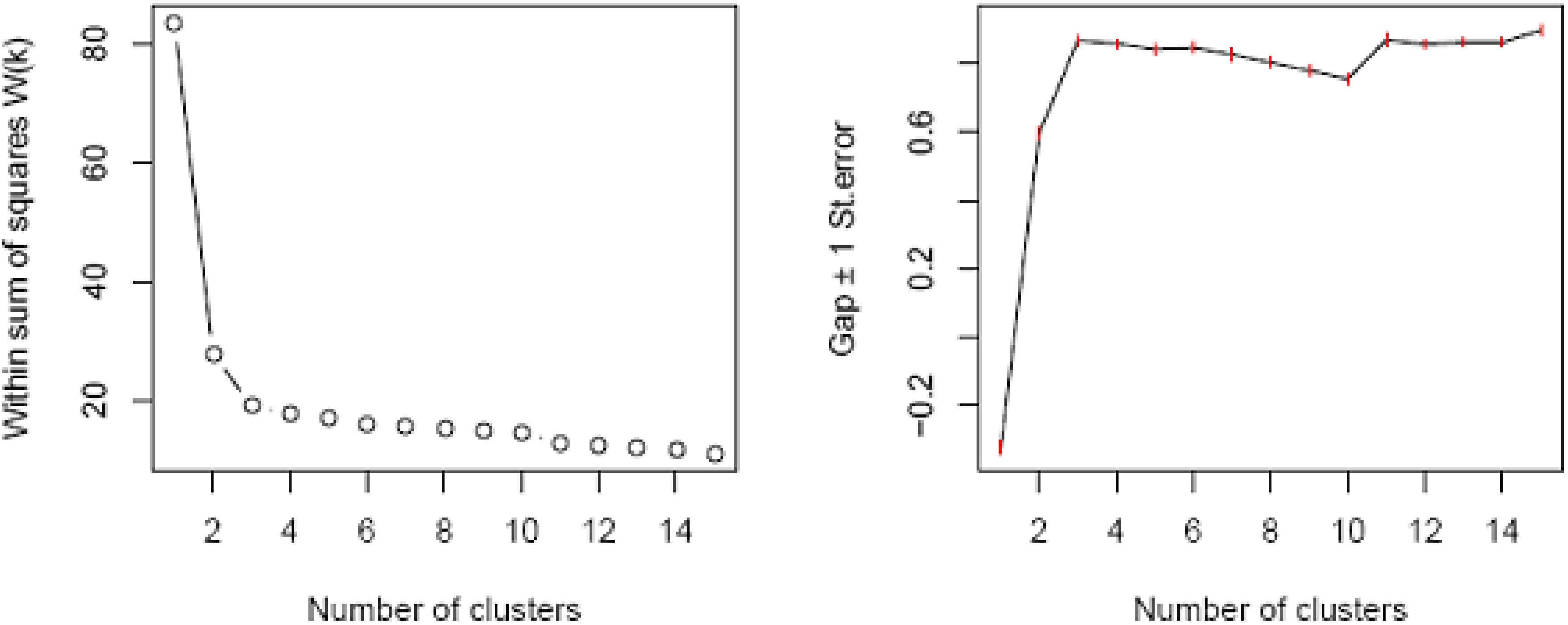
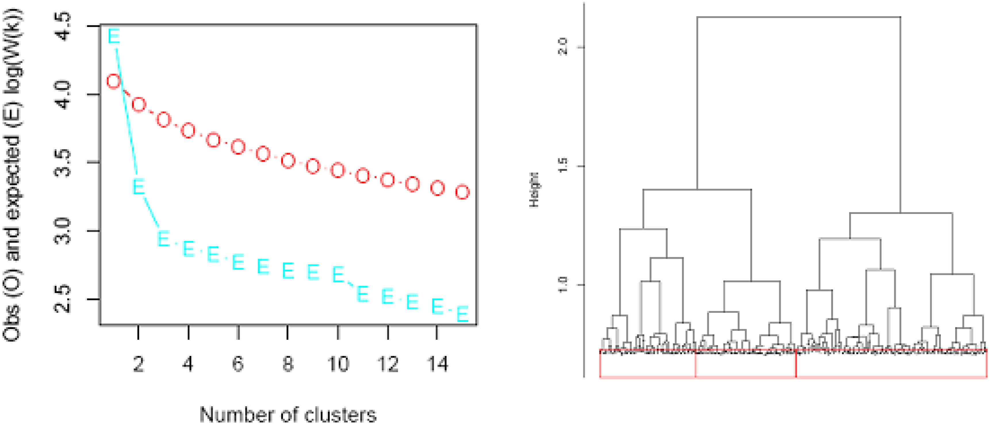
Clustering households

Key steps in agglomerative clustering of categorical data are the creation of a proximity matrix, the clustering of the proximity matrix, and the selection of appropriate groupings to form the clusters.
The study employed the “daisy” method based on the Gower metric, a proximity measure most suitable for data sets containing categorical variables [10]. An agglomerative hierarchical clustering (“agnes”) using the Ward method then defined the cluster tree [11], because of its tendency to minimise information loss and to reduce the likelihood of small clusters. Ward’s clustering requires a Euclidian proximity matrix. A transformation of the Gower proximity matrix into a Euclidian is available with the lingoes function in the package ade4 [12].
Clustering large number of variables has the potential to include variables that do not contribute to the cluster structure. Such variables are masking the “real” underlying structure, so that the clustering result reflects noise in the data (see e.g., [13]). This masking problem has had recent attention with a range of algorithms available to identify noisy variables [14]. However, none of these methods has the ability to incorporate categorical variables directly, so they do not satisfy the demands of this study. Other options can incorporate resampling methods, but these rapidly become very demanding of computer resources, so that there is only limited scope for including these in an approach for datasets with many categorical variables.
One reasonably old technique, the cophenetic correlation coefficient or CPCC [15] is able to deal with categorical/nominal variables, as it compares the proximity measure with the hierarchical clustering output using a Pearson correlation (as discussed e.g., in [16]). Here I use this measure to identify which variable combination produces an acceptable CPCC, via a forward selection procedure, and define the cut off level to be ≥0.7 for the study site Kukar. Table 1 provides the selected variables from the study site Kukar as an example. It shows the cophenetic correlation coefficient from a forward selection procedure. A coefficient smaller than 0.7 led to the exclusion of associated variables. Using this variable selection procedure provides a list of variables that warrant further investigation by the researcher in terms of their relevance to the research question at hand. For example, owning a generator may not be important to your livelihood if you live in an area with reliable mains connection.
Table 1. Variable combinations resulting from a forward selection procedure based on the cophenetic correlation coefficient at the study site Kukar.
Number of variablesCophenetic Correlation CoefficientVariables added
1Initial variableOther.assets
20.99Recreation.income
30.98Daily.wage.rate
40.96People.in.HH
50.94Car.truck
60.92Kerosene.stove
70.89Children.7.16.years
80.86Honey.income
90.83Income.per.wage.earner
100.81Woodfuel.stove
110.78total.monthly.workdays
120.76Air.conditioner
130.73Wild.pig.income
140.71Total.years.education
150.70Born.in.East.Kalimantan_new
160.82Born.in.Kalimantan
170.84Born.in.district_new
180.85Refrigerator.freezer
190.84Fishing.boat
200.83Rattan.income
210.82Motorbike
220.82Children.under.7
230.81Ethnic.group
240.80Days.worked.past.month
250.79Months.of.work
260.78Total.monthly.wage.income
270.78House
280.77Boat.engine.
290.76.Wage.earners
300.75Social.networks.income
310.74maxdisttravelled
320.73Small.TV
330.73Fruit.tree.income
340.72Handphone
350.71Fish.income
360.70HHincome.per.person
370.69Timber.income
380.69Kijan.income
390.68Washing.machine
400.67Total.monthly.HH.income
410.66Education.income
420.65Roads.income
430.65Rubber.income
440.64Water.pump
450.63Large.TV.
460.62typeofwork
470.61Computer
480.59Generator
490.58Education.level
500.56Gas.or.electric.stove
A second issue is the definition of final clusters. Identifying the final clusters can be subjective if based only on visual interpretation. While there are a range of approaches and methods to determine “ideal” cluster number in unsupervised and supervised classification (see e.g., [17,18]), I used the Gap statistic to identify the cluster number because it also considers a single cluster (i.e., no division of the data) in the comparison, which most other methods are unable to do [18]. The Gap statistic identifies the optimal cluster number in relation to a reference distribution, and based upon the within-cluster dispersion. Simulations showed the superior performance of this statistic over other cluster number assessment methods [19]. Although the initially proposed Gap statistic does not focus on methods for categorical variables, it is suitable for hierarchical clustering of categorical variables. For the purpose of this study, I extended the method to incorporate the daisy algorithm. Figure 1 provides an example of the gap measures.
Figure 1. Example of gap statistics using daisy and the Gower metrics. The number of best clusters in this example is three based on the highest gap value and distance between observed and expected log(W(k)).
Sustainability 02 00533 g001aSustainability 02 00533 g001b
To identify the best cluster number, it is important to (i) maximise the distance between the observed and expected values of within-cluster dispersion (here expressed as log(W(k)) between the data (O) and reference data (E), (ii) find the number of clusters where the within-sum of squares of W(k) trajectory is reduced, and (iii) find where the Gap statistic is largest, while taking into consideration non overlapping standard deviations. If standard deviations overlap, chose the smaller cluster number.
In the example of study site Kukar in Figure 1, five clusters display a low within-sum of squares (W(k)), and a high gap value. This coincides with one of the largest gaps between the observed and expected log(W(k)) values and is also observed in the dendrogram showing three main splits. However, the split in the dendrogram is close to further branching, so one could feasibly argue for further cluster separation. Here the gap statistics provide an advantage as further splits are unsupported because more clusters do not provide a market improvement when taking into consideration Gap standard error.
Practical considerations meant that clustering included all variables and that it also provided site specific results on livelihood variables. Hence, the identification of HH types involved clustering variables of the entire, cross-site dataset and a second clustering of variables using only site specific livelihood data. Combining these two cluster outputs then yielded the final HH types. The coding for these HH types reflects this approach, such that, for example, 1Samarinda1 would be all households located in the overall cluster 1 at site Samarinda, where these households are members of the sites specific to overall cluster 1. While this step is required for the subsequent interviews, results are not of interest for this paper, so will not be discussed further.

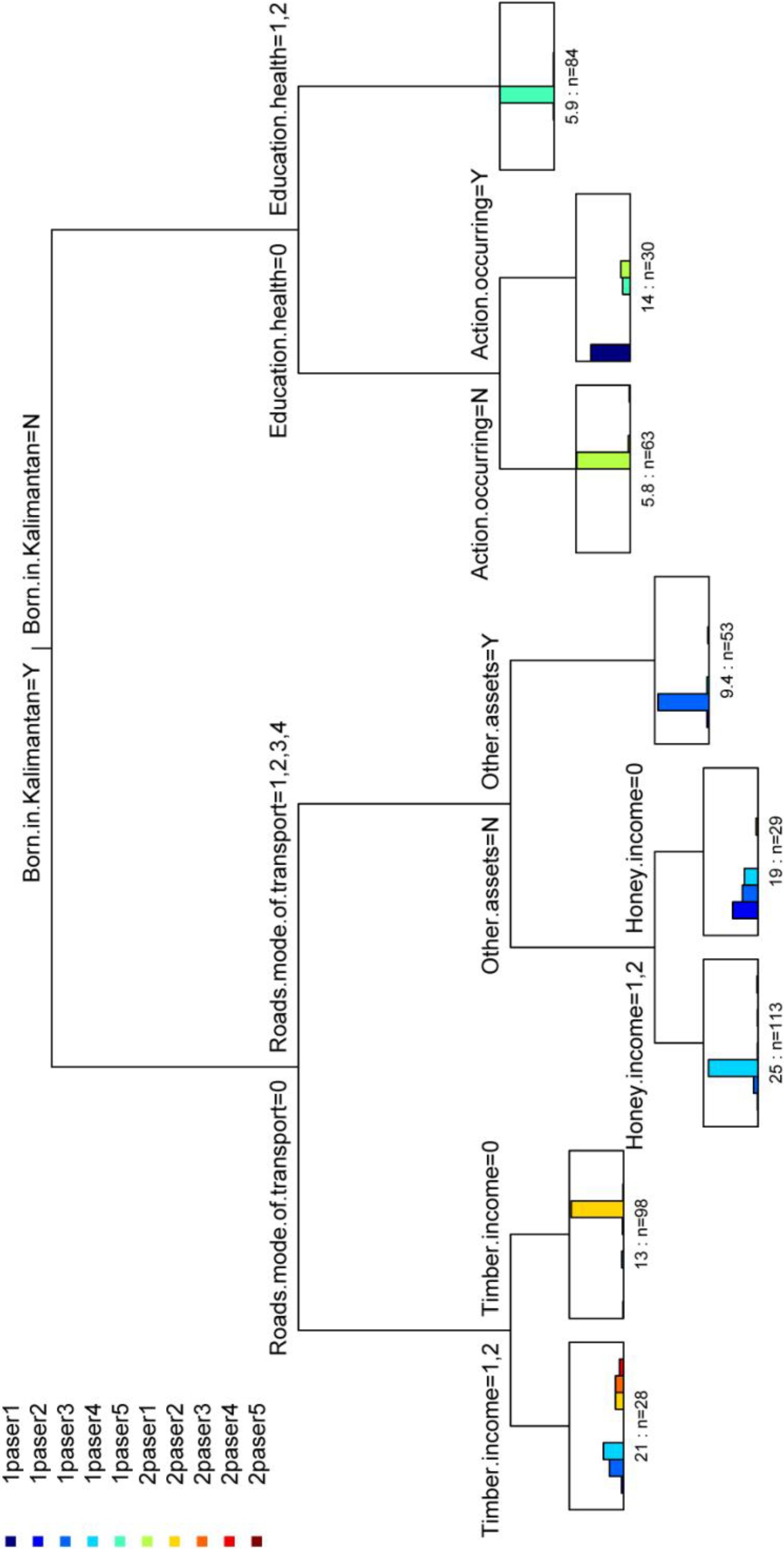
Decision tree analysis for allocating new households

Identifying these HH types formed the groupings to which new households needed to be allocated for the intensive interviews. This was easily achieved using a decision tree approach [20], which enabled identification of important underlying variables. Here I used the mvpart library, a multivariate decision tree approach [21], and a binary allocation (i.e., cluster present or absent) of the clusters at a specific site as explanatory variable. This approach provides useful variable cut-off levels to assign the new households into the HH groupings. It further provides frequency distributions of the HH groupings for each decision tree end node.

Extract important variables underlying clusters

The clustering incorporated a two part approach, which rendered it more difficult to extract the variables driving the HH types. Additionally, it is also not trivial to identify the contributions categorical variables make to the clusters. This is a common problem in machine learning and prediction approaches, where an unknown optimal explanatory (predictor) fit is derived from the data. This fit then enables the identification of variable importance. While it is an advancement in the categorical data analyses, the procedures are still missing a way of calculating inference for the important variables [22]. There are potentially options for extending this method using bootstrap and other resampling methods to generate inference statistics. However, such an implementation would require significant computing resources when working with larger datasets, so is out of the reach of most users. Strobl et al. outlined that the current random forest approach for variable inference is unsuitable for mixed-categorical data and that there is need for variable inference method development that can be implemented into the cforest approach, though this is future work [23].
This research incorporated a recent development to identify important variables. It extends the random forest decision tree approach [24] for estimating the relative importance of categorical variables [25]. While the random forest approach and its extension do not provide an inferential measure of variable importance, the latter method overcomes the issue of bias related to categorical variables that have different numbers of categories [23]. Variable importance in our context is the prediction accuracy for each group of random (cforest) trees based upon the varimp algorithm of the R package party [25]. This algorithm reports the average of the out-of-the-bag data portion and the predictor permutation accuracy difference, for all trees normalised by the standard error [24], but without the categorical variable bias.
The cforest approach requires that there is no missing data in the response variable. Data preparation for the response variable involved replacement of missing values through imputation to avoid the alternate solution of deleting all information on HHs with missing data values. Imputation for the variables involved replacing the missing value with the median for this variable. Given that the proportion of missing values was mostly below 4% (except for three, which where below 7%) and the predictors were uncorrelated, this approach is unlikely to introduce significant bias into the analysis [26].

3. Results

This section provides the details and results on the analysis steps outlined in the previous sections. It also gives examples of the output.

3.1. HH Classes from Clustering

The first step in the clustering was to identify household groupings over all sites on all variables. In the second step, site specific household clustering on livelihood variables yielded a second grouping. The combination of both these clusterings then defined the final HH types for the sites (Table 2). These household types subsequently formed the basis for building a decision tree with which to place new households into these groupings. The decision tree provides the means of classifying new HHs into the existing clusters—a step required for determining HH typology during the interview stage. This then enables the linking of the detailed HH information for the agent development with the HH types at each study site.
Table 2. Household clusters based on overall clustering (first number in HH type) and site specificity (site name and second number in HH type), and number of households per HHtype (n). Overall clusters were three.
SiteHH typeHH per HH type (n)
Balikpapan1balikpapan1239
1balikpapan224
1balikpapan310
2balikpapan1121
2balikpapan22
2balikpapan31
Balikpapan Total 397
Kubar1kubar19
1kubar268
1kubar351
1kubar47
1kubar55
2kubar145
2kubar2229
2kubar392
2kubar44
2kubar511
2kubar61
Kubar Total 522
Kukar1kukar162
1kukar226
1kukar38
1kukar42
2kukar191
2kukar2102
2kukar370
2kukar451
2kukar528
Kukar Total 440
Paser1paser125
1paser231
1paser3132
1paser484
1paser547
2paser167
2paser294
2paser37
2paser42
2paser59
Paser Total 498
PPU1ppu1179
1ppu214
1ppu376
2ppu14
2ppu2132
2ppu379
PPU Total 484
Samarinda1samarinda119
1samarinda315
2samarinda1402
2samarinda28
2samarinda314
2samarinda420
Samarinda Total 478
Grand Total 2819
Most decision tree endnodes in Figure 2 lead to clearly distinguished HH types. For example HH type 1paser5 on the first endnode from the right is clearly identified through following the decision nodes on the right decision tree arm. When following the decision tree nodes along this path (i.e., Born.in.Kalimantan = N, Education.health = 1,2) all new cases belong most likely to 1paser5. In the first and fourth endnode from the left in Figure 2 it is difficult to distinguish HH types based on the distribution of the bars in the charts, which means that any new case aligning with these endnodes based on these decision tree paths are not suitable for a clear classification into any of the HH types. This highlights the advantage of using a decision tree method as it allows assessment of how a new HH aligns with the existing classification. In practice this could help decide if a HH with such a variable combination should be part of the interview procedure.
Figure 2. Decision tree example showing the levels for variable cut-offs that lead to specific HH types. Ordinate of boxes show the proportion of HH in a specific HH type. The HH types in the boxes are aligned from left to right following the order of the legend.
Sustainability 02 00533 g002

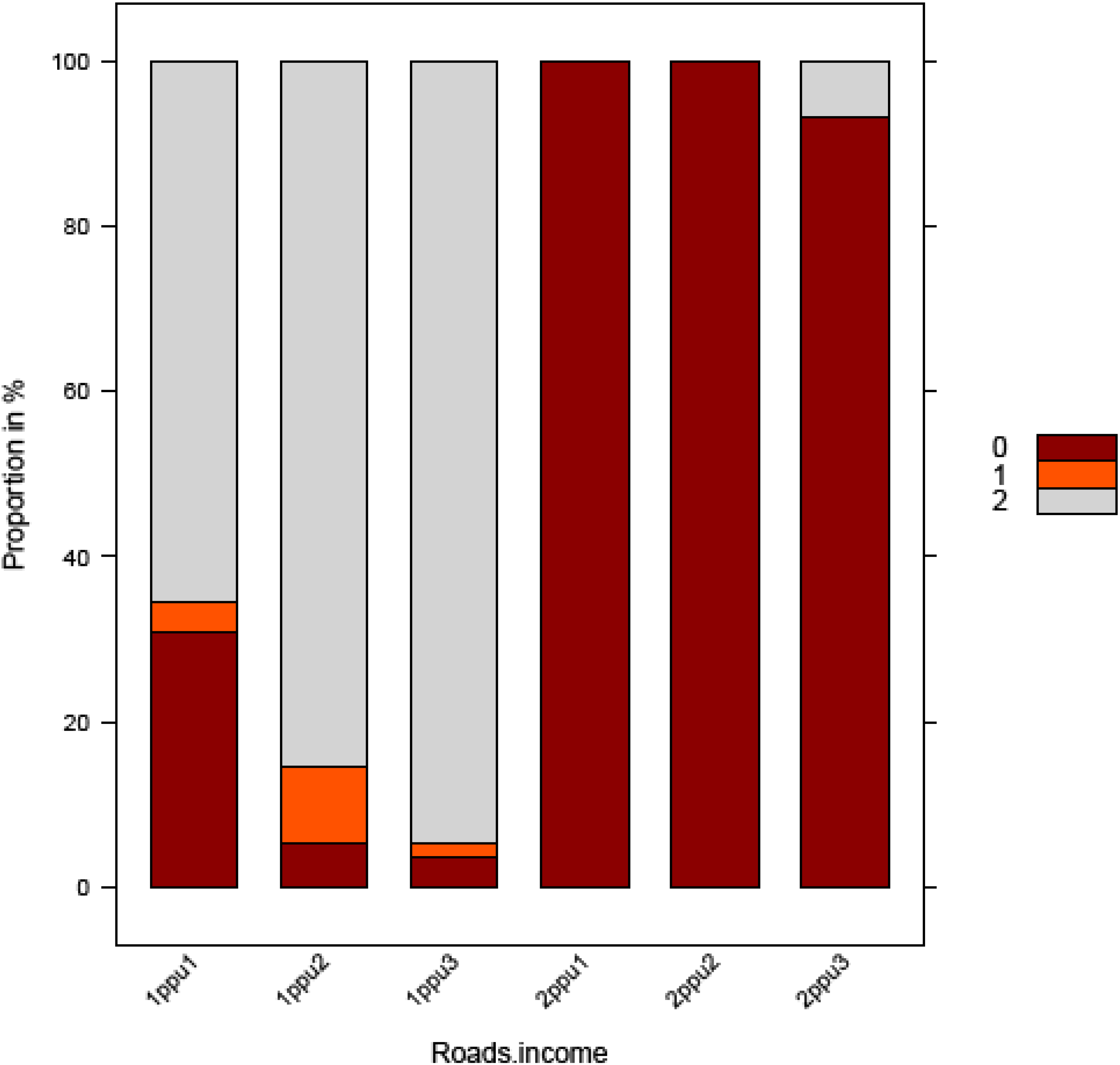
3.2. Extraction of Most Important Variables

While a decision tree is ideal to describe groupings and to develop a pathway for placing new HH into the existing groups, it is less rigorous in identifying important variables. These variables are required for developing agents’ characteristics. The extraction method provides a measure to assess the relative importance of the variables describing a grouping, based upon a probabilistic approach. Variable importance in classifications is conveniently determined through the extended random forest approach, which incorporates multiple decision trees. The importance measure of the variables is based on their contribution to the optimal tree structure [24,25]. In our case Roads contribution to income, Born in Kalimantan, Born in east Kalimantan, Born in district and ethnic group were the most frequently selected variables. Roads contribution to income (coded Roads.income) occurred at five sites as an important variable (Table 3). To investigate this in more detail, we can look at how HHs rated Roads.income at, for example, PPU (Figure 3). Here, HH types 1ppu1, 1ppu2 and 1ppu3 featured people who rated the roads’ contribution to income as important or very important (value 1,2). In 1ppu2 approximately 70% of people saw a road’s contribution to income as important or very important while the remainder found roads not important for their income generation, and for all people in 2ppu1 and 2ppu2 and over 90% of 2ppu3 roads were unimportant for their income (Figure 3). A next step, for example, to interpret underlying economic drivers could be to compare other livelihood variables for the HHs that had a similar rating here.
Table 3. Important variables extracted with the unbiased random forest algorithm.
SiteVariableVariable importance
BalikpapanBorn.in.East.Kalimantan0.0118
Born.in.district_new0.0091
Born.in.Kalimantan0.0080
Roads.income0.0016
Small.TV0.0008
KubarEthnic.group0.0176
Rubber.income0.0167
Other.assets0.0142
Born.in.Kalimantan0.0129
Born.in.district_new0.0081
Born.in.East.Kalimantan0.0079
typeofwork0.0033
Months.of.work0.0024
Roads.income0.0017
Boat.engine.0.0015
Education.level0.0012
Fishing.boat0.0009
Hornbill.income0.0008
Fish.income0.0004
KukarBorn.in.Kalimantan0.0154
Born.in.East.Kalimantan_new0.0134
Born.in.district_new0.0115
Fish.income0.0081
Ethnic.group0.0061
Boat.engine.0.0047
Fishing.boat0.0037
Months.of.work0.0006
typeofwork0.0001
PaserBorn.in.Kalimantan0.0258
Roads.income0.0215
Timber.income0.0197
Born.in.East.Kalimantan0.0186
Honey.income0.0154
Born.in.district_new0.0142
Generator0.0081
Other.assets0.0061
Fruit.tree.income0.0054
Education.income0.0050
Fishing.boat0.0040
Ethnic.group0.0034
Boat.engine.0.0032
typeofwork0.0015
Water.pump0.0014
Air.conditioner0.0003
Rubber.income0.0003
Washing.machine0.0001
PPURoads.income0.0298
Born.in.East.Kalimantan0.0207
Born.in.Kalimantan0.0174
Born.in.district_new0.0082
Ethnic.group0.0054
Education.income0.0015
Social.networks.income0.0013
SamarindaBorn.in.Kalimantan0.0277
Born.in.East.Kalimantan0.0229
Roads.income0.0214
Ethnic.group0.0076
Born.in.district_new0.0068
Education.income0.0063
Social.networks.income0.0041
typeofwork0.0007
Figure 3. The contribution of roads to income (Roads.income ratings: 0 = roads do not contribute to income, 1 = roads contribute somewhat to income, 2 = roads contribute significantly to income) as an important variable at ppu.
Sustainability 02 00533 g003

4. Discussion and Conclusion

The objective of the research was to develop a strategy for dealing with categorical variables from surveys and for providing information to agent based model development. Here it was important to (i) create groupings of similar households, (ii) describe these households in a way that enabled the classification of new households into these groups and (iii) provide a list of the most important variables underlying the HH classification.
The strategy used survey data to classify households into representative groups and used these groupings to select households for detailed interviews. These interview results can now serve the development of agents representative of these groups. The strategy allowed cost reduction by replacing expensive interviews with rapid surveys. It also provided the means for the development of a limited number of agents (represented by the groupings) and enabled tracing of important variables related to these groupings.
The mixed character of the survey variables (i.e., nominal, ordinal and interval scaled variables) and the large number of variables meant that an analysis with conventional methods would have resulted in significant statistical issues related to the loss of degrees of freedom stemming from the number of predictor variables and their categories [“the curse of dimensionality”, 27]. Also the combination of the overall and site specific clustering required a different strategy to identify variables underlying the groupings.
Another difficulty is related to excluding noisy variables in a cluster analysis of categorical nature. While there are a range of recent methods for numerical analyses [14], none of these deal with mixed categoric and numeric data satisfactorily. The cophenetic correlation coefficient is a possibility, but falls short when there is an increasing number of variables and cases, because of the increased time required to calculate proximity matrices and cluster matrices, and to assess all possible variable combinations (see e.g., [28]). While used as a shortcut, forward or backward variable selection mechanisms have drawbacks as they do not consider all possible variable combinations. The latter would increase the time required even more in the calculation, which can with modern desktop computers require several days. While this is less an issue with high capacity computers, it is more difficult to implement for normal desktop users, the people most likely to be applying this strategy. Here I showed an example of using the CPCC for the study site Kukar, however, faster approaches similar to those examined in Steinley & Brusco [22] and extended to deal with categorical variables are highly desirable. Also, as an alternative, the time investment required to identify important variables through variable exclusion and examination of cluster separation would have been extensive.
The decision tree approach enabled the user to make relatively quick decisions about what new HHs should be part of the intensive interview process, through identifying a new HH’s alignment with the HH types. This was possible using the proportions associated with each HH location in the decision tree. There, decision combinations leading to a HH type at a tree branch with low frequencies could result in rejection of the HH for detailed interviews. Besides providing the classification ability, it also made it possible to determine the strength of a decision tree end node in defining a particular HH type. Hence, the user could make an informed decision for including or rejecting a new HH for intensive interviews in a comparatively short time frame. This is generally not available when using conventional methods.
Conventional analysis of categorical survey data is fraught with issues of non-normality, and multivariate methods relying on parametric statistics are less robust in their results than non-parametric ones. This study has employed a new strategy of analysing survey data that (i) enables the identification of clusters, (ii) allows the extraction of important variables underlying these groupings and (iii) develops a decision tree for allocating the cluster membership of new HH. The combination further enables categorical data analysis without limitations of conventional statistical approaches requiring normality or multivariate normality. However, there are limitations of this strategy, which are related to increased computer demand when variables have a large number of categories. While this may be only a time issue that disappears with increasing computer power, a high number of variable categories may also be an indication that survey and questionnaire design require further attention. For example, it is possible to reduce the number of categories in a variable by recoding and rethinking the answer the variable can provide.
In a recent study, support vector machines, a machine learning classification method, showed best performance when compared with other supervised learning methods including decision trees [29]. However, their work was concerned with a binary automated classification and the performance of the bagged support vector machines improved with the reduction of predictors. This means that the application of support vector machines was limited for the purpose of this study, because here it used many predictor variables and multiple classes of the response variates.
The application of the new strategy has potential for a range of survey data (including in other disciplines such as biology and medicine), where building a typology and prediction of type membership for new cases is required. It moves away from frequentist statistical approaches for identifying important variables, to a modelling approach. This circumvents conventional issues related to mixed categoric and numeric data analysis and puts the variable extraction into a probabilistic framework with a focus on variables most likely to drive the cluster membership. However, while it is possible with the employed method to identify variable importance ranking, currently it is not reasonably possible to establish the significance and inference between the important variables [22]. While there may be the option of using bootstrapping for identification of inferences, no readily available approach exists and there would be a trade-off against computer time requirements, which are already considerable using the current algorithm.

Acknowledgements

The reviews of Nick Abel, Samantha Stone-Jovicich, and Petra Kuhnert improved the manuscript markedly, as did the comments of anonymous reviewers. I thank Silva Larson and Alex Kutt for their helpful comments and discussions, and Sally Way for edits of the earlier manuscript. Karin Hosking provided editorial input of the final version. Peter Hairsine’s experience in scientific writing at CSIRO contributed significantly to the conception of this paper.

References and Notes

  1. Janssen, M.A.; Carpenter, S.A. Managing resilience of lakes: A multi-agent modeling approach. Conserv. Ecol. 1999, 3, 15. [Google Scholar]
  2. Carpenter, S.A.; Brock, W.A. Spatial complexity, resilience and policy diversity: Fishing on lake-rich landscapes. Ecol. Soc. 2004, 9, 8. [Google Scholar]
  3. Bousquet, F.; Le Page, C. Multi-agent simulations and ecosystem management: A review. Ecol. Model. 2004, 176, 332. [Google Scholar] [CrossRef]
  4. Bohensky, E.; Smajgl, A.; Herr, A. Calibrating behavioural variables in Agent-Based Models: Insights from a case study in East Kalimantan, Indonesia. In Modsim 2007; Oxley, L., Kulasiri, D., Eds.; Modelling and Simulation Society of Australia and New Zealand: Canberra, Australia, 2007. [Google Scholar]
  5. Venables, W.N.; Ripley, B.D. Modern Applied Statistics with S; Springer: New York, NY, USA, 2002. [Google Scholar]
  6. Borgatti, S.P. Anthropac 4 Methods Guide; Analytic Technologies: Natick, MA, USA, 1996. [Google Scholar]
  7. Santos, L.; Marings, I.; Brito, P. Measuring subjective quality of life: A survey of Portos’ residents. Appl. Res. Qual. Life 2007, 2, 51–64. [Google Scholar] [CrossRef]
  8. R Development Core Team. R: A Language and Environment for Statistical Computing; R Foundation for Statistical Computing: Vienna, Austria, 2008. [Google Scholar]
  9. Ferrier, S.; Guisan, A. Spatial modelling of biodiversity at the community level. J. Appl. Ecol. 2006, 43, 393–404. [Google Scholar] [CrossRef]
  10. Kaufman, L.; Rousseeuw, P.J. Finding Groups in Data: An Introduction to Cluster Analysis; Wiley: New York, NY, USA, 1990. [Google Scholar]
  11. Struyf, A.; Hubert, M.; Rousseeuw, P.J. Clustering in an object-orientated environment. J. Stat. Softw. 1997, 1, 1–30. [Google Scholar]
  12. Chessel, D.; Dufour, A. B.; Thioulouse, J. The ade4 package-I-One-table methods. R News 2004, 4, 5–10. [Google Scholar]
  13. Schinka, A.J.; Velicer, W.I.; Weiner, I.B. Handbook of Psychology: Research Methodologies in Psychology; John Wiley and Sons: Somerset, NJ, USA, 2003. [Google Scholar]
  14. Steinley, D.; Brusco, M.J. Selection of variables in cluster analysis: An empirical comparison of eight procedures. Psychometrika 2008, 73, 125–144. [Google Scholar] [CrossRef]
  15. Sokal, R.R.; Rohlf, F.J. The comparison of dendrograms by objective methods. Taxon 1962, 11, 33–40. [Google Scholar] [CrossRef]
  16. Tan, P.N.; Steinbach, M.; Kumar, V. Cluster analysis basic concepts and algorithms. In Introduction to Data Mining; Addison-Wesley: London, UK, 2006. [Google Scholar]
  17. Milligan, G.W.; Cooper, M.C. Methodology review: Clustering methods. App. Psych. Meas. 1987, 11, 329–354. [Google Scholar] [CrossRef]
  18. Gordon, A. Null models in cluster evaluation. In From Data to Knowledge; Gaul, W., Pfeiffer, D., Eds.; Springer: New York, NY, USA, 1996; pp. 32–44. [Google Scholar]
  19. Tibshirani, R.; Walther, G.; Hastie, T. Estimating the number of clusters in a data set via the gap statistic. J. Roy. Statist. Soc. B. 2001, 63, 411–423. [Google Scholar] [CrossRef]
  20. Breiman, L.; Friedman, R.A.; Olshen, R.; Stone, C.J. Classification and Regression Trees; Wadsworth International Group: Belmont, CA, USA, 1984. [Google Scholar]
  21. De’ath, G. Multivariate regression trees: A new technique for modeling species-environment relationships. Ecology 2002, 83, 1105–1117. [Google Scholar]
  22. Van der Laan, M. Statistical inference for variable importance. Int. J. Biostat. 2006, 2, 1–31. [Google Scholar]
  23. Strobl, C.; Boulesteix, A.; Zeileis, A.; Hothorn, T. Bias in random forest variable importance measure: Illustrations, sources and a solution. BMC Bioinformatics 2007, 8, 1–21. [Google Scholar] [CrossRef] [PubMed]
  24. Breiman, L. Random forests. Mach. Learn. 2001, 45, 5–32. [Google Scholar] [CrossRef]
  25. Hothorn, T.; Hornik, K.; Zeileis, A. Unbiased recursive partitioning: A conditional inference framework. J. Comput. Graph. Stat. 2006, 15, 651–674. [Google Scholar] [CrossRef]
  26. Harrell, F.E.J. Regression Modelling Strategies: With Applications to Linear Models, Logistic Regressions and Survival Analysis; Springer: New York, NY, USA, 2001. [Google Scholar]
  27. Bellman, R.E. Adaptive Control Processes; Princeton University Press: Princeton, NJ, USA, 1961. [Google Scholar]
  28. George, E.I. The variable selection problem. J. Am. Stat. Assoc. 2000, 95, 1304–1308. [Google Scholar] [CrossRef]
  29. Pino-Mejías, R.; Carrasco-Mairena, M.; Pascual-Acosta, A.; Cubiles-de-la-Vega, M.D.; Muñoz-García, J. A comparison of classification models to identify the fragile X Syndrome. J. Appl. Statists. 2008, 35, 233–244. [Google Scholar] [CrossRef]

