The System Dynamics of U.S. Automobile Fuel Economy

Department of City and Regional Planning, University of North Carolina at Chapel Hill, New East Building, Campus Box #3140, Chapel Hill, NC 27599-3140, USA
Sustainability 2012, 4(5), 1013-1042; https://0-doi-org.brum.beds.ac.uk/10.3390/su4051013
Submission received: 2 April 2012
/
Revised: 24 April 2012
/
Accepted: 9 May 2012
/
Published: 18 May 2012
Abstract
:This paper analyzes the dynamics of U.S. automobile gasoline consumption since 1975. Using background literature on the history of domestic fuel economy and energy policy, I establish a conceptual model that explains historical trends in adoption of increased fuel economy. I then create a system dynamics simulation model to understand the relationship between increased fuel economy standards and potential changes to gas tax policies. The model suggests that when increases in mandated fuel economy are not conducted in an environment with rising fuel costs, fuel economy improvements may be directly counteracted by shifting tastes of consumers towards larger automobiles with lower fuel economy.
1. Introduction
The United States’ transportation system has distinguished itself as one of the most gasoline-reliant systems in the world; U.S. gasoline consumption has increased throughout the past five decades, jumping from 1.9 billion barrels in 1960 to 4.9 billion barrels in 2010 [1]. As the single most important daily mode of transportation, the demographic layout of U.S. cities and businesses has been changed since the diffusion of the American automobile. However, the use of gasoline as the primary fuel for the overwhelming majority of automobiles in America has not come without problems. Over the last several decades, the United States has witnessed an enormous volatility in the market for gasoline, derived from both the lack of stability in foreign countries that produce oil, and in the collusion of those countries to increase prices worldwide [2,3]. Adding to this volatility, concerns about domestic pollution, excessive resource consumption, and climate change have created many delicate economic and social issues that surround the market for gasoline.
As a result, although policy makers have identified dependence on imported oil as an urgent energy, economic and national security concern, the gap between domestic consumption and domestic production is more than 50 percent of total oil consumption; by 2030 imports are predicted to reach 68 percent of U.S. petroleum consumption [4]. Complicating this are a number of policy problems that result from federal fuel economy standards and taxes, including concerns over vehicle safety, comfort, and consumer choice, and the economic impacts of regulation on automobile sales [5].
In this article, I present a system dynamics computer simulation model of American automobile fuel economy in order to better understand the relationship between increased fuel economy standards and potential changes to gas tax policies. System dynamics modeling allows us to simulate different policy strategies in order to understand system feedback effects, such as those that may result from recent efforts to increase fuel economy (e.g., [6]), and proposals for increases in fuel taxes [7].
The model suggests that, when increases in mandated fuel economy are not conducted in an environment with rising marginal driving costs (fuel costs), fuel economy improvements may be directly counteracted by shifting tastes of consumers towards larger automobiles with lower fuel economy.
This article begins with a review of literature on U.S. gasoline consumption and fuel economy policy, focusing on the two primary initiatives for reducing domestic gasoline consumption, including (1) the Corporate Average Fuel Economy Standards (CAFE) for cars and light trucks and (2) gasoline taxes paid by consumers at the pump. Next, I use historical data and trends to form a dynamic hypothesis of U.S. automobile fuel economy, which facilities examination of non-intuitive feedback effects from mandated increases in fuel economy. I then use this dynamic hypothesis to create a system dynamics model that attempts to replicate the structure of this system and the historical trends that have been observed since the early 1970s. In analyzing this model, sensitive testing is performed on variables that effect gasoline consumption. Finally, I conclude by offering recommendations for further action and research on fleet-level automobile fuel economy.
2. Background
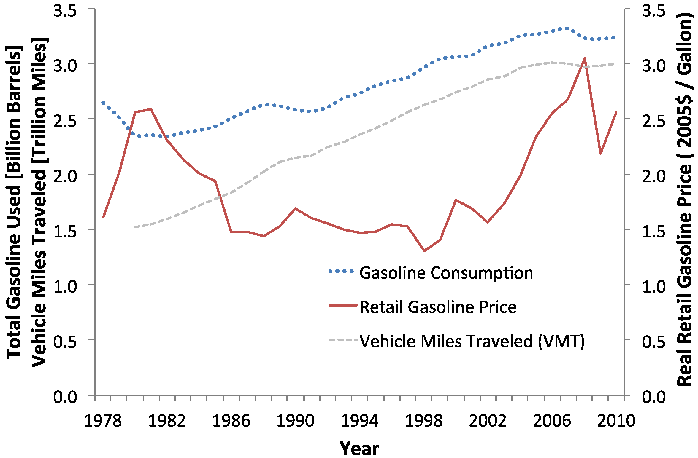
In 1973, the Organization of Petroleum Exporting Countries (OPEC) used its cartel power to triple U.S. crude oil prices from ~$20 to ~$59 per barrel (2010$) (Figure 1; [8,9]). Although manufacturers and drivers discovered ways to economize following this spike in oil prices, policymakers felt that market forces would fail to adequately reduce American energy consumption and dependence on foreign oil [10]. Therefore, in 1975, the Federal Energy Administration, an executive agency created to “assist in developing policies and plans to meet the energy needs of the Nation, (15 U.S.C. 61B §761),” extended controls to domestic crude oil and refined-product prices, reducing them well below world prices, and far below prevailing estimates of future prices [10].
Although artificially low prices undercut conservation efforts, Congress was unwilling to allow prices to rise due to fears that rising prices would have negative effects on the overall rate of inflation and on distributional equity. Instead, Congress focused on the reduction of oil consumption by automobiles as an efficient way of decreasing the U.S. reliance on foreign oil. Rather than allowing fuel prices to rise, policy was directed towards higher fuel-economy standards to influence the design of new fuel-efficient automobiles [10].

Starting in 1978, the Energy Policy and Conservation Act of 1975 (42 USC §6201) imposed the Corporate Average Fuel Economy (CAFE) standards on all automobile manufacturers operating in the United States [13]. Under CAFE, the average fuel consumption of the fleet of cars and light trucks [14] sold by a manufacturer in a given year could not exceed a specified level. The standards are a weighted average, meaning that manufacturers can continue selling a mix of efficient and inefficient vehicles; the fuel-inefficiencies of large cars (high cost to make fuel-efficient) are offset by efficiencies of small cars (inexpensive to increase efficiency to exceed CAFE standards).
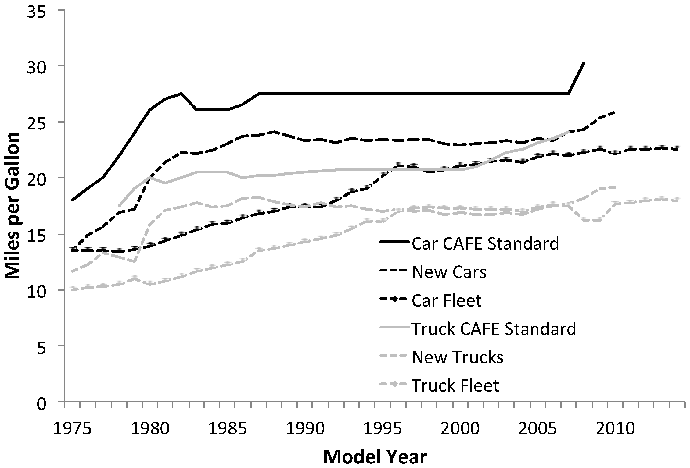
The historical progression of the CAFE standards and fuel economy of the American auto fleet is shown in Figure 2, starting with the major efficiency increases during the tumultuous period following the 1970s oil embargo. At the time CAFE standards were enacted, light trucks were primarily used as commercial and agricultural work vehicles and represented a relatively small portion of the automobile market. Thus, a lower CAFE standard was established for light trucks (including most sport utility vehicles (SUVs) and all mini-vans) than for passenger cars [15]. In the 1980s, when OPEC stopped restraining output and real gasoline prices began to decline, CAFE standards were no longer increased. Stagnation in CAFE standard growth continued from 1990 to 2011 (until 2005 for trucks), when congress passed an increase in the standards to 30.2 MPG (ramped up from 20.7 MPG in 2005 to 24.1 MPG in 2011).
More recently, the U.S. Congress passed the Energy Independence and Security Act of 2007 [16], mandating that the combined fleet of all passenger cars and light trucks sold by all manufacturers in the U.S. in model year 2020 exceed 35 MPG. Under the 2008–2011 standards [17], fuel economy standards are now based on continuous mathematical formula related fuel economy to vehicle “footprint” size (the product of multiplying wheelbase by track width). Under this model, smaller trucks have higher fuel economy targets than larger trucks, and manufacturers making larger trucks are allowed to meet a lower overall target. With no remaining requirements for manufacturers to meet any particular overall actual MPG target, overall fuel economy will depend on the mix of vehicles purchased by consumers. In 2009, regulations covering model years 2012–2016 were issued requiring average fuel economy increases to 39 MPG for cars and 30 mpg for trucks (35.5 MPG fleet average) by 2016. In 2011, the U.S. Environmental Protection Agency (EPA) and Department of Transportation (DOT) and U.S. DOT issued the most recent regulations increasing fuel economy to 54.5 MPG by 2025 [18]. To give this context to other countries around the world, the European Union has proposed a 64.8 MPG target by 2020, while Japan has proposed a 55.1 MPG standard by 2020 [19].
Figure 2.
Corporate Average Fuel Economy Standards (CAFE) standards and fuel economy of car/truck fleet and new cars and trucks [20].
Figure 2.
Corporate Average Fuel Economy Standards (CAFE) standards and fuel economy of car/truck fleet and new cars and trucks [20].

2.1. Has CAFE Worked?
Has CAFE has been successful in reducing the United States’ consumption of oil? To simply point to increased fuel economy in the U.S. over the past thirty years as CAFE’s success may confound the effects of the fuel economy standards with the symptoms that caused them to be instituted. In order to properly analyze the fuel consumption dilemma, we must look at the actual results of the CAFE program and examine briefly how the standards have altered gasoline consumption.
I can break the question of CAFE's effectiveness into three components. First, how have CAFE standards affected the fuel economy (miles per gallon; MPG) of new cars being sold? Second, how have the changes in new cars affected the composition and age of the overall car and light truck fleets that are in use today? Finally, to what extent have changes in fuel economy been offset by increases in the vehicle-miles traveled (VMT) of the average American driver? Addressing these three questions will help to explore the policy issues that surround the CAFE standards and their implementation.
The CAFE standards have greatly improved the fuel economy of new cars, on average. During the late 1970s, lighter cars, greater horsepower-to-weight ratios, smaller engine sizes, front-wheel drive, and other engineering improvements led to a 50 percent increase in average fuel efficiency of the new vehicle fleet [21,22]. However, most of this efficiency improvement occurred in the late 1970s, during which real retail gasoline prices doubled from approximately $1.35 in 1972 to around $2.59 in 1981 (2005$; [8]). This price increase makes it difficult to determine whether CAFE was responsible for increased fuel economy, or whether it was purely market forces causing increased demand of fuel economy vehicles. Only when prices fell in the 1980s did the major automakers begin to have difficulty meeting the CAFE standards (i.e., getting consumers to purchase high-MPG cars).
Based on Figure 1 and Figure 2, it could be argued that CAFE standards rose only when the market would demand greater fuel economy from new automobiles being introduced into the fleet. However, CAFE standards stopped rising when they began to require manufacturers to produce more fuel-efficient cars than consumers wanted to buy. Although automakers worked within the CAFE regulatory framework and attempted to maximize the features valued by drivers, consumers stopped factoring fuel economy as highly into their new vehicle choices when fuel prices fell in the 1980s [10]. Since consumers were purchasing enough low-MPG vehicles that automakers would fail to meet the minimum fleet-average MPG CAFE standards, automakers reacted with huge price markups on inefficient vehicles to compensate [8].
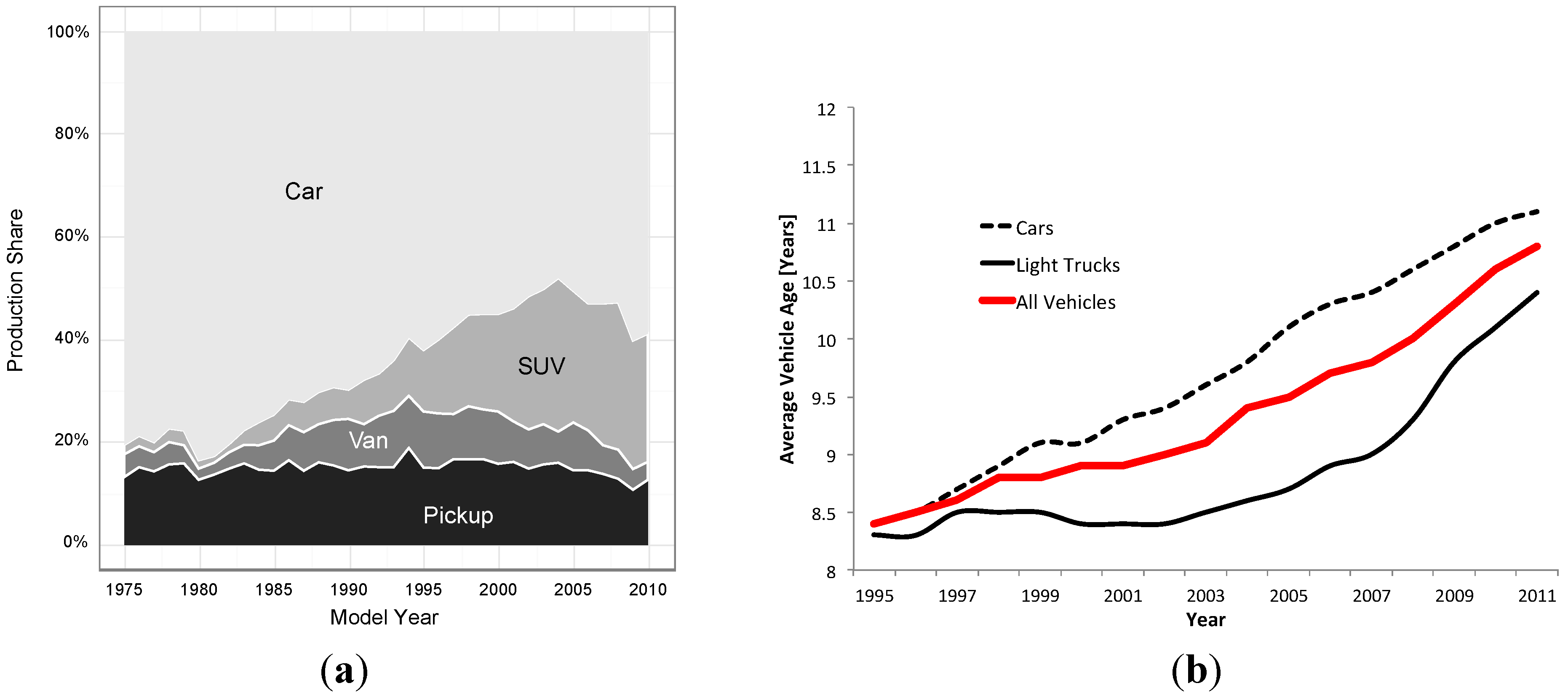
During this period, when larger, less efficient vehicles became more expensive, consumers reacted in unexpected ways (Figure 3). Many consumers continued to purchase more expensive, low-MPG vehicles, which were much more appealing (and viewed as safer and more comfortable), while a modest fraction began purchasing cheaper, high-MPG vehicles. However, many consumers reacted by purchasing vans, Sports Utility Vehicles (SUVs) and light trucks, or by continuing to drive their older cars. Between 1977 and 1995, the average age of registered vehicles rose from 5.6 years old to 8.3 years old [23]; stated differently: in 1980, 8% of all registered cars were retired from the active fleet, while only 6% were retired in 1993 [10]. These data imply that the growth of the new-vehicle market was slowed due to the fact that existing vehicles were made to last longer by their owners. The only recent data available on average vehicle age is shown in Figure 3b.
Figure 3.
(a) New vehicle market share by vehicle type (figure reproduced from Environmental Protection Agency (EPA) report [22], p. v); (b) Average Vehicle Age (1995–2011) [24].

In 1980, light truck sales made up 18% of the total sales of consumer automobiles (~10.9 million total vehicles). By 1993, truck sales had risen to 37%, and by 1997 surpassed those of cars [8]. As of 2010, trucks made up over 52% of the U.S. light vehicle market [25]. Much of this market share transition has been explained by Bradsher [26], who explains how manufacturers reacted to falling gasoline prices, particularly by providing the lead in producing more SUVs that were not required to meet the CAFE standards for cars, changing them to be more car-like, and advertising in the earlier years of their growth (late 1980s through the 1990s) to convince consumers that SUVs were strong substitutes for cars.
I can address the structural cause of fuel consumption dynamics by looking more directly at how CAFE has affected driving habits. While CAFE made new cars more expensive in the short term, it did little to raise the marginal cost of driving. As the economy of new cars doubled, the gasoline component of the costs of driving one mile decreased by half, thereby leading to a “rebound effect,” whereby consumers are incentivized to drive farther and more often ([27]; although more recent research has estimated this effect to be declining over time [28]). Complicating our understanding of the dynamics of fuel economy and VMT is the growing number of vehicles and drivers on the road. Concurrent with increasing urbanization in the United States between 1980 and 2010, the total number of vehicle-miles traveled (VMT) nearly doubled to ~3 trillion miles, which increased transportation-related gasoline consumption by 37.4% (~883 million barrels per year) [11,12].
CAFE opponents often argue that fuel economy increases will be very expensive unless the size and weight of new cars are decreased significantly, thereby leading to decreased safety and comfort [29]. The National Highway Traffic Safety Administration (NHTSA) has studied CAFE's effects on weight and size reduction, concluding that the standards increased fatalities by ~2000 per year between 1985 and 1993 [30]. More recent work has confirmed that weight decreases can increase fatality rates [31]. Opponents have also historically pointed out that CAFE increases force automakers to manufacture and sell cars that are not only expensive (expensive fuel economy research and development), but are met with low public demand when gas prices are low, since “…consumers are more interested in vehicle size and utility than in fuel economy [32].”
2.2. The Role of Gasoline Taxes
The CAFE standards are almost entirely directed at the supply side of the automobile market (e.g., CAFE does not incentivize auto maintenance after purchase). The introduction of a gas tax as a method of reducing gasoline consumption has been touted as an efficient solution to many of CAFE’s side effects, since the CAFE standards are less effective at sending price signals to affect consumer decisions when gas prices are low [8]. In view of this major policy shortcoming, would higher fuel prices elicit a greater consumer response to the attempt to decreased gasoline consumption? Research has shown that both drivers and automakers respond to increased fuel prices by adjusting the fuel economy of the cars they purchase or manufacture.
The link between gasoline consumption and price can be explored by looking at the enormous literature that has developed on estimating the price elasticity of gasoline Ef. While estimates of this value figures vary widely, meta-analyses [33,34] have estimated short-term elasticities of −0.01 to −0.57 (mean = −0.25), while long-term estimates are between 0 and –1.81 (mean = –0.64; [34]). One of the same meta-analyses also shows that per vehicle VMT, reacts to gasoline prices changes with a similar elasticity (between −0.69 and −0.33, mean = −0.51; [34]). Evidence has shown that higher fuel prices induce improvements in the technical fuel economy of a vehicle after about a four-year lag due to the time that manufacturers require to adjust vehicle their vehicle designs [10]. Additionally, research has calculated that manufacturers adjust the price of new vehicles based on gasoline prices, offsetting future discounted gasoline price increases or decreases incurred by consumers. For example, in response to a one dollar increase in gasoline prices, Langer and Miller [35] found an average reduction of $792 for cars and $981 for SUVs (price changes for trucks and vans were not statistically significant), which, substantially offset the discounted future gasoline expenditures incurred by consumers [36].
Many arguments against gasoline taxation that are based on macroeconomic merits assume that the revenue generated by the tax would not be filtered back into the economy, either by reductions in other taxes, or by increased governmental services to reduce the costs of externalities caused by the use of gasoline [8,10]. Cashell and Lazzari [37] argued that if the CAFE program was ended, and a 25-cent fuel excise tax was introduced, the U.S. GDP would decrease by 0.1–0.2% for approximately 3 years. More recently, the Congressional Budget Office [38] estimated that a 46 cent-per-gallon increase in federal gasoline taxes would cost the U.S. economy $2.9 billion annually (or roughly ~$10 per person per year).
However, how realistic are large increases in gasoline taxes? History has shown that raising prices is politically unfavorable. Voters and automakers would fight government efforts to impose higher gasoline, road, and other travel taxes if they perceived that there was no alternative to driving. In spite of this, however, in 2010 the Simpson-Bowles commission [39] proposed a 15-cent increase in federal gas tax (currently 18.4 cents a gallon for gasoline and 24.4 cents for diesel fuel) starting in 2013 (phased in by one cent every three months). While never instituted, it is one of many recent proposals to increase federal gas taxes over time.
3. Fuel Economy Dynamic Hypothesis
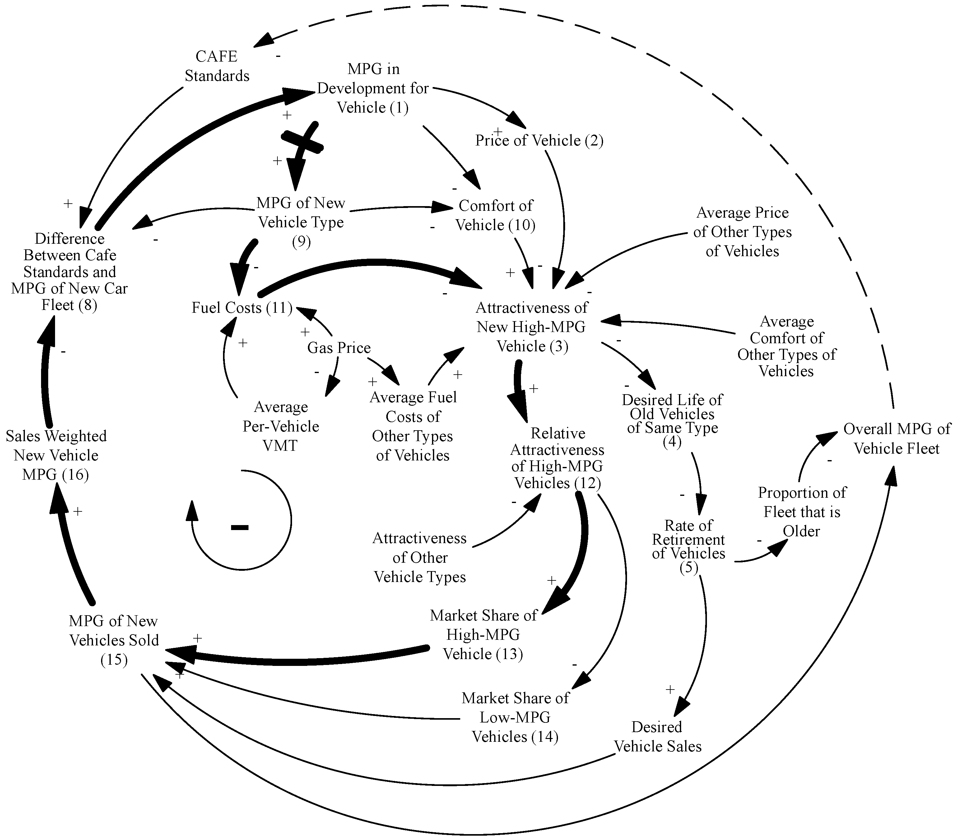
A dynamic hypothesis uses the datasets discussed in the last section to map out the causal connections between variables in a systemic context, whose visual depiction is commonly known as a Causal Loop Diagram (CLD; [40]). These causal connections commonly form feedback loops, whereby changes in a given system are often the cause of the system itself, rather than shocks to the system that are delivered exogenously. The complete dynamic hypothesis is shown in Figure 4 with individual variables denoted in parentheses (for high-MPG vehicles only–others are denoted as ‘other vehicle types’ for graphical simplicity). It is important to note that positive links (+) denotes that a change in one variable will change another variable in the same direction, while negative links (–) denote that a change in one variable will have the opposite effect on another variable.
In order to create the major loops of the causal loop diagram, it is important to first observe several of the intervening causal effects of the CAFE standards that have non-intuitive effects. Although there are numerous factors affecting the attractiveness of new vehicles [29,41], I begin by collapsing these into three general factors: fuel economy, vehicle price, and vehicle comfort. Although these may be overly broad, they are useful factors for broadly exploring the causal dynamics of this system. To build the dynamic hypothesis, I also collapse the spectrum of available vehicle types into two categories, high- and low-MPG vehicles. However, for the actual quantitative system dynamics model, these two categories are explicitly used for cars, and another truck category is added to distinguish trucks, vans, and SUVs based on different applicable CAFE standards [21].
We know that there is a positive effect on the fuel economy of the new vehicle fleet when automaker research and development towards fuel economy increases. We have represented this as MPG in Development for Vehicle (1; R&D). To present this in a causal fashion, we can imagine the MPG of the new vehicle fleet as a supply chain, with R&D represented as a flow of MPG into the new vehicle fleet. However, as R&D increases, the price of the new vehicle is likely to increase as well [8], while the comfort of the new vehicle (10) will, ceteris paribus, decrease due to lowered weight and feature reduction to facilitate increased fuel economy [42]. This in turn, means that an increase in Comfort of Vehicle (10) will cause an increase in Attractiveness of new High-MPG Vehicle (3).
Figure 4.
Dynamic hypothesis of automobile fuel consumption (focusing on high-miles per gallon (MPG) vehicles section only). The feedback loop shown in bold shows the theorized shift towards high-MPG cars as goal seeking behavior when CAFE standards are increased. However, as I will show, viewing this loop in isolation ignores the effects of gas price, and changes in comfort and vehicle price from fuel economy development.

Conversely, however, an increase in MPG in Development for Vehicle (1) will cause a decrease in Comfort of Vehicle (10). This behavior alone explains much of the un-expected dynamics that have generated the stagnation of CAFE standards growth between when gas price dropped in the mid-1980s to the early-2000s; if fuel economy research and development is not coupled with high gasoline prices, the negative effect of increased price and decreased comfort on the attractiveness of a new vehicle can far outweigh the effect of increased fuel economy.
To understand the effects on a vehicle’s ability to be sold, I assert that as one type of automobile becomes more attractive, its market share grows, which lowers the market share of other types of automobile. In the case where fuel-efficient vehicle attractiveness increases, the attractiveness of other vehicle types fall, which then increases the fuel economy of the new vehicle fleet (defined as all vehicles sold in the most recent year).
Concurrently, as a vehicle type becomes less attractive, the rate at which old vehicles of that type retire falls. This was illustrated when the average age of registered cars rose from 6.6 to 8.3 years between 1980 and 1993 [43]. Here, we can see the effect that the attractiveness of an automobile (3) has on both its desired life (4); the period before it is eventually retired to a junkyard) and on its market share of new vehicles being purchased.
The introduction of any change in CAFE standards causes a discrepancy between the current new-fleet fuel economy and the economy necessary to satisfy the new standards. To close this gap, R&D begins, and, after legislative and development delays (the time in necessary to put the new standard into law and for automakers to alter fuel economy), the new vehicle MPG adjusts accordingly. This adjustment is seen in the MPG of New Vehicle Type (9), which closes the gap between the new CAFE standard and the MPG of the new car fleet.
This model treats the CAFE standards themselves as exogenous variables. Modeling CAFE standards endogenously would necessitate a method of representing the political pressures that influence federal actions towards fuel economy. Therefore, a far more productive way of including the CAFE standards in this model is by viewing them as an exogenous variable whose increases are politically associated with high gas prices. The model does account for the fact that as gas prices increase, the average vehicle-miles-traveled (VMT) per car drops [8], thereby causing a decrease in total fuel costs. However, until this system is modeled quantitatively, it is not possible to determine whether gas prices or the effect of gas prices on total VMT influences total Fuel Costs (11) more.
It is important to stress here that a major shortcoming of this model (and as I will discuss in the conclusions, an important area of future research) is that it does not incorporate feedback from increased fuel prices (through gas taxes or exogenous price spikes) to increased fuel economy. Fuel economy changes are instead modeled as entirely the product of changing CAFE standards. Under this view, the model explicitly asserts that the CAFE standards are the only mechanism that explicitly drives fuel economy R&D (I do not directly consider very complex relationship between gas taxes, consumer tastes, and R&D that each auto company defines for themselves). In Figure 4, the dotted line represents a political (not modeled) link that represents one of the considerations that lawmakers face when posed with an increase to the CAFE standards.
One important limitation of this model is that there is no explicit link modeled between Fuel Costs (11) and fuel economy improvement (1). That is, the model is not able to capture feedback between exogenous gas price spikes and the impetus for fuel economy improvements (i.e., MPG increases not mandated under the CAFE standards). Although this is an important dynamic, I leave this work to future research on this topic, as modeling the link between demand and supply of fuel economy will necessitate substantial additional model feedback structures.
The final piece of the dynamic hypothesis concerns the interaction between the CAFE standards and the fuel economy of the overall fleet. We can assert that the fuel economy of the overall fleet is a weighted average of the vehicle fleet still on the road. The causal link between the attractiveness of new vehicles and average vehicle life affects the overall fleet fuel economy by altering the number of new (and theoretically higher-economy) vehicles sold.
One of the most important interactions depicted within this dynamic hypothesis is the relationship between fuel economy Research and Development (1) and total Fuel Costs (11). If R&D is not coupled with high gasoline prices, the negative effect of increased price and decreased comfort on the attractiveness of a new vehicle far outweighs the effect of increased fuel economy. This dynamic implies that decoupling CAFE standards and gas prices could be a main cause of market share migration to other low-economy vehicle types, thereby undermining the effect of fuel economy R&D altogether. In the next section, I use this dynamic hypothesis to construct a model that explains the historic behavior of automobile gasoline usage in the United States.
4. Modeling Automobile Gasoline Usage
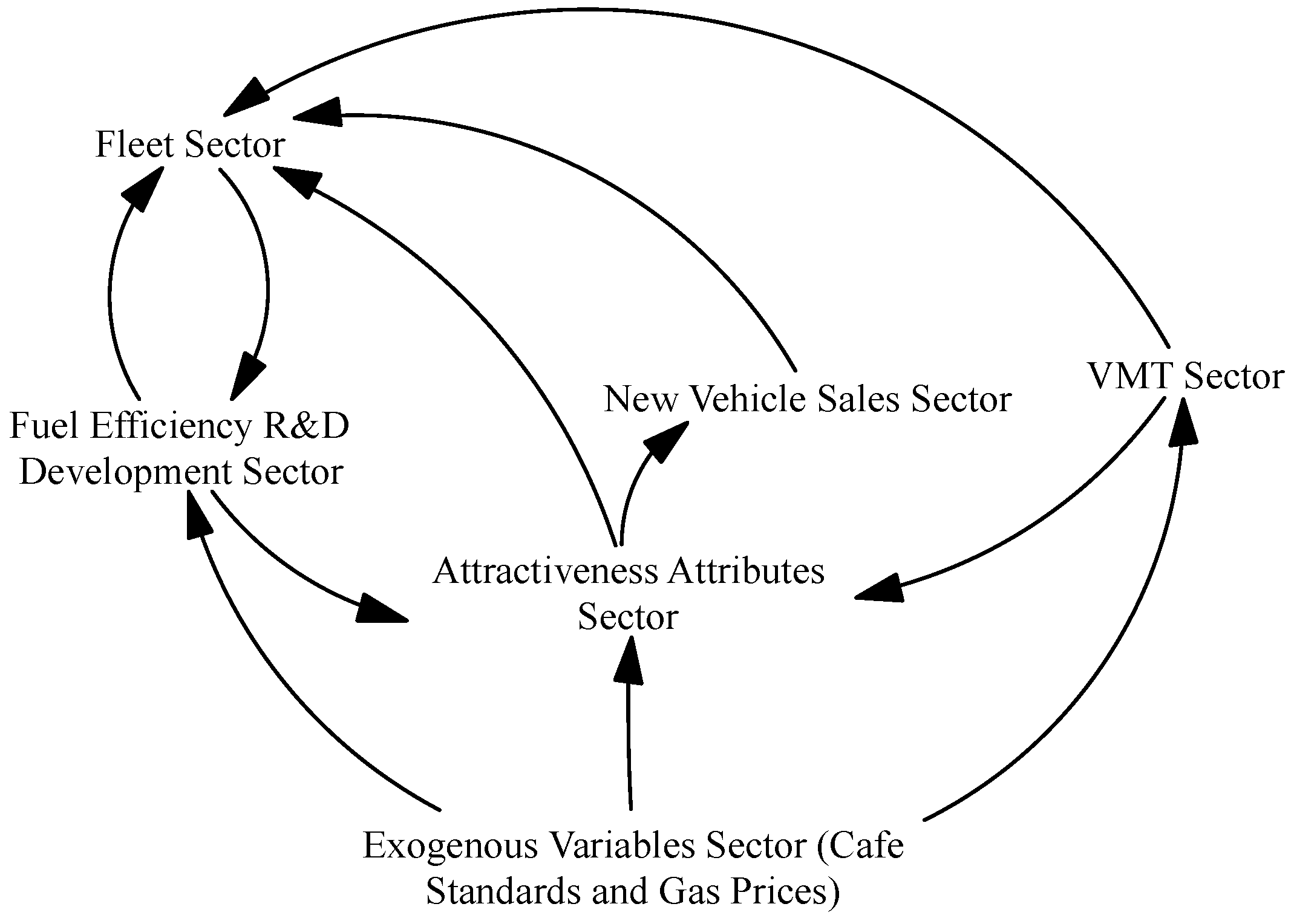
The model structure is divided into the following sectors, which together generate the structural interaction diagram in Figure 5:
Figure 5.
Sector structure for automobile gasoline usage model.

- Exogenous Variables—The major exogenous variables that we can classify here are gas prices and the CAFE standards. To properly model gas prices, I would need to employ a complex commodity model to generate the proper oscillatory behavior of gas prices. In the case of the CAFE standards, we see that they have been highly associated with the rate at which gas prices change (see Figure 1 and Figure 2).
- Fuel Economy R&D Development Sector—The R&D necessary for closing the gap between current new-fleet fuel economy and the economy mandated by the CAFE standards.
- New Vehicle Sales—Uses data from the attractiveness attributes sector and returns market share fractions for each vehicle type.
- Attractiveness Attributes—The three broad factors contributing to vehicle attractiveness: vehicle price, fuel costs, and comfort.
- Fleet—The overall make-up of the vehicles that are currently on the road, as modeled in three categories, high-MPG Cars, low-MPG Cars, and trucks.
- VMT—Computes the average per-vehicle VMT based on (1) lifestyle changes in the United States over the last several decades; and (2) gas prices, which alter the amount that the average person is willing to drive. Each of these sectors is discussed in more detail in the following sub-sections.
4.1. Exogenous Variables and Data Sets
Although I use extensive data for model calibration (which is discussed below), only two datasets feed exogenous data in the model, gas prices and CAFE standards, which are taken directly from the National Highway Traffic Safety Administration (NHTSA; [21]) and the U.S. Department of Energy (real prices, normalized to year 2005 dollars; [1]).
It is important to note that throughout the model, I use a first-order smooth (delay of 3 years for producers and two years for consumers) of gasoline prices to eliminate rapid gasoline prices fluctuations and only send price signals when there are large gasoline price changes over a long period of time. When consumers purchase a car (or when automakers produce a car) I assume that the fuel prices will only factor into decision-making processes if gas prices remain at a high level over a long period of time. Therefore, I utilize the system dynamics technique of using a first-order smooth over a time period of 3 years for producers and 2 years for consumers.
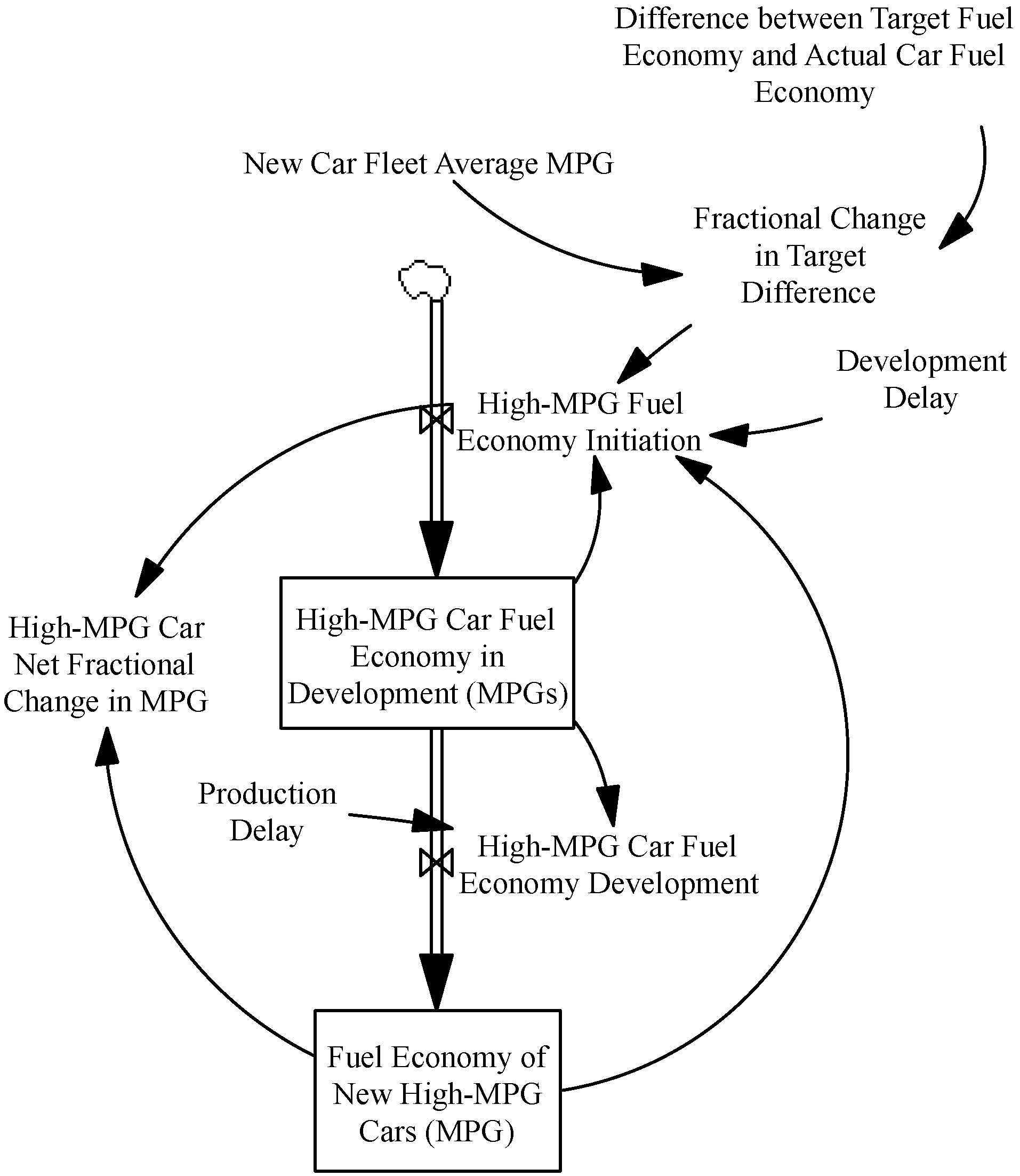
4.2. R&D/Fuel Economy Development Sector
The structure of the fuel economy R&D development sector (Figure 6) can be thought of as a supply chain, where any increases in R&D act to increase the flow of R&D already in production (measured as MPG/car/year), which flows into the New-Fleet MPG. This means that increases in R&D slowly increase the economy of new vehicles (after delays). A legislative delay of one year slows the flow of new R&D into the pipeline, which represents delays in setting CAFE standards and automakers re-allocation of R&D resources between projects.
I divide the new vehicle fleet into three vehicle types; the first is trucks, which include any vehicle under 8,500 lbs. that is not defined by the EPA as a car. Trucks are the largest, heaviest, and least fuel-efficient vehicle type. The second vehicle type is high-MPG Cars, which the smallest, lightest and most fuel-efficient cars that exceed the CAFE standard (typically compacts and sub-compacts). The third vehicle type, low-MPG Cars, lies between high-MPG Cars and trucks, and includes all cars that do not exceed the CAFE standards.
To divide new R&D among the different vehicle types, I simply assert that new R&D starts are based on the difference between the light truck CAFE standard and the new truck fleet MPG. For cars, I simply take the weighted average of car sales to determine the allocation of new R&D for the two car types. I replicate the structure in Figure 6 for low-MPG Cars and for trucks (accounting for different target values associated with truck CAFE standards). Finally, it is important to note that the High-MPG Car Net Fractional Change in MPG variable is used as a proxy for calculating the rate at which MPG R&D increases car price [44].
Figure 6.
Change in fuel economy research and development (R&D) for high-MPG cars.

4.3. New Car Sales Sector
To explore how new vehicle types gain and lose market share, I create an index for determining each vehicle type’s relative attractiveness to that of other new vehicles:
![Sustainability 04 01013 i001]()

Using this renormalized Relative Vehicle Attractiveness index, it is easy to determine if a vehicle’s market share will increase or decrease. Values greater than one signify that market share will increase, values <1, signify market share decrease, and values = 1 signify market share that is in equilibrium (any dynamics in the sector are driven by the other vehicle types).
As a baseline, the initial market shares of all vehicle types were calculated using estimates of real-world data in 1970 (data from 1975, the earliest available; [45]), which constitute the initial Normal Vehicle Fraction, a smoothed value (over 5 years; altered by increased attractiveness of a vehicle type) which forms the base line for calculating each vehicle type’s market share. Constraining each vehicle type’s market share below 5% or rise above 90%, the following equation is used to calculate the Indicated Truck Fraction (which is also re-normalized by dividing by the average values so all vehicle type market shares sum to one):
![Sustainability 04 01013 i002]()

4.4. Attractiveness Attributes Sector
It is now necessary to define and elaborate on each of the factors that I model as influencing a consumer’s decision to purchase a new vehicle. I model these as a series of three ratios, including
- 1) Fuel Costs—The Average Per-Vehicle VMT divided by the MPG of Each Vehicle Type’s New Fleet, and multiplied by the Gasoline Price Smooth Seen by Customers (2005 U.S. dollars). The model then calculates the ratio of this value to the fuel costs experienced by the vehicle fleet as a whole.
- 2) Comfort/Safety—In order to model the effect of vehicle comfort on vehicle attractiveness, the model must account for the effects of fuel economy development on the comfort and safety level of a vehicle. Lowered weight is associated with lower comfort due to less accessories adding to vehicle weight, and lower safety due to smaller crumple zones and lack of safety features in the higher mileage automobile [29]. An important dynamic takes the opposite relationship of that of fuel costs and attractiveness; since the fuel economy of a new vehicle is closely tied to its comfort (or perceived comfort), as the fuel economy of a vehicle increases relative to other vehicle types, the model asserts that the comfort of the vehicle decreases. The model divides the MPG of Vehicle Type’s New Fleet by the New Fleet Average MPG across All Vehicle Types. This calculation yields the inverse of the relative comfort when compared to other vehicle types (this is to keep the functional form of Equation 3, below, consistent);
- 3) Vehicle Price—A multiplier is calculated that yields the ratio of current vehicle price to 1970 vehicle price using Effect of MPG Development on Vehicle Costs. While this calculation of vehicle price is vastly simplified from reality, it reflect the fact that increased fuel economy standards do increase vehicle costs substantially, therefore leading to the type of complex, non-intuitive effects on market share that have been seen historically [46].
Initially, graphical functions were explored to connect each of these ‘ratios’ to vehicle attractiveness. While the causal relationships suggested that these functions were likely to be logistic in nature, the graphical functions were found to be extremely sensitive and largely arbitrary (little data informs these relationships). A solution was found by taking each one of these ratio factors as an input into a compounded (negative) logistic growth function:
![Sustainability 04 01013 i003]()

Where K is a threshold or ‘carrying capacity’ value (taken as 10; [47]), and Fratio, Cratio, and Pratio are the Fuel Costs (F), Comfort and Attractiveness (C), and Vehicle Price (P) ratios, respectively. To parameterize this function, three factors rF, rC, and RP are established logistic equation growth rates, and AF, AC, and AP are established as ‘initial’ values for the three vehicle attractiveness determinants. Given that data on the r and A parameters are unavailable (primarily since they represent previously unmeasured relationships), optimization/calibration procedures embedded in the Vensim DSS 5.11A software [48] were used to fit these parameters to available historic datasets on new vehicle market share and fuel economy, fleet-wide fuel economy (for trucks and all cars), gasoline consumption, and vehicle miles traveled (VMT).
4.5. The Fleet Sector
The Fleet Sector constitutes a tracking system for the make-up of vehicles currently on the road. By multiplying the market share of each vehicle type (from the New Car Sales Sector) by the Desired Vehicle Sales, the fleet sector calculates the new purchases of each vehicle type. The total Desired Vehicle Sales is the number of vehicles of any type that can be sold in a year, constituting the consumer market for new vehicles (Time to Adjust Fleet =1 year):
![Sustainability 04 01013 i004]()

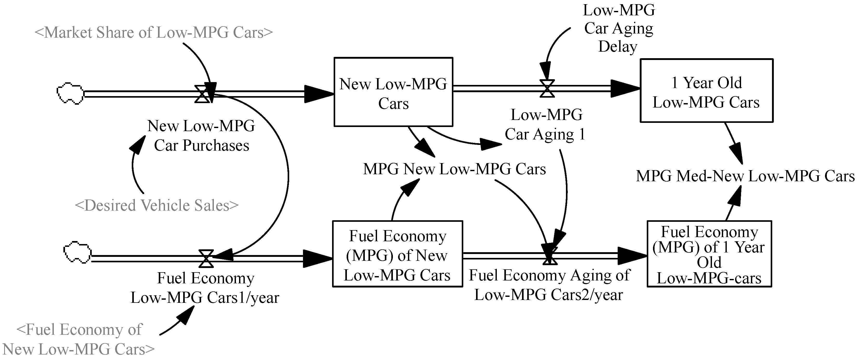
It is now imperative to age the vehicles by using a system dynamics structure known as an aging-chain [40]. Accompanying this, I can track each model-year’s MPG by using a co-flow structure, which allows the model to track an attribute that is associated with another variable that is flowing between stocks. This structure is shown in Figure 7, where the lower aging-chain tracks a variable whose units are MPG-cars, which facilitates accounting for fuel economy development. Each aging chain contains four stocks (not shown completely in Figure 7), and any change in the average life of a car must be modeled by modifying the outflow from the final stock in the aging chain.
Figure 7.
Aging-chain and co-flow structure to track vehicle demographics.

As the attractiveness of new vehicles changes, the average age of old vehicles changes with the changing willingness of the public to purchase new automobiles. Therefore, as the Attractiveness of Old Vehicles increases, the lifespan of older vehicles increases as well, which I calculate using a third-order smooth of each vehicle type’s new counterpart. The attractiveness of the new vehicle is then divided by the attractiveness of the old vehicle, and used as input into a linearly decreasing graphical function called the Effect of Attractiveness on Retirement. This relationship asserts that increases in new vehicle attractiveness above that of an old vehicle lead to vehicle retirement rate increases, and decreases in vehicle lifespan. When the attractiveness of new and old vehicles is the same, the life of an older vehicle remains the same as its initial value.
By modeling the feedback between the attractiveness of new cars and the retirement rate of older cars, my goal is to gain insight into the dynamics affecting vehicle life increases during the 1980s and 1990s [23], and continues today [49]. The last sector looks at the amount that the average consumer drives, which coupled with the Fleet Sector, will allow us learn how automobile usage has changed historically, and may change in the future.
4.6. The VMT Sector
The VMT sector calculates the average VMT that consumers drive their vehicles per year by multiplying the base VMT (1970 value) by an Effect from Gas Prices on VMT and adding another Effect from Lifestyle Changes on VMT (increases due to other macroeconomic and cultural factors; e.g., highway expansion and other lifestyle changes).
The Effect from Gas Prices on VMT uses the mean price elasticity of per-vehicle VMT assessed by a survey of literature by Goodwin, Dargay, and Hanly [34], such that when gasoline price increases by 1%, VMT declines by 0.51%. The Effect from Lifestyle Changes on VMT [50] takes the form of simple ramp function that increases the per-vehicle VMT by 45 miles per year, as calculated from [20] and [51]. The historical values produced mirror real world values accurately and we see a constant increase in per-capita VMT (see Figure 1). Now that the system dynamics model is complete, I will simulate the model and examine the results in the next section.
5. Model Results and Policy Analysis
I begin model testing and policy analysis by calibrating the model to historical data. Next, I discuss the model’s historical base run–the model parameters that best represent the actual historical behavior of MPG development. This is followed by testing of a series of several different scenarios, including increased future CAFE standards and gasoline taxes, a scenario that equilibrates car and light truck CAFE standards, and a final scenario that combines several of the other scenarios to test their synergistic behavior.
5.1. Model Calibration
Model calibration was performed using the Vensim DSS 5.11A optimization procedure, which fits parameters to data sources using a pay-off function. To fit the payoff function to each data variable, the variable was weighted using the inverse of the maximum data value of the data [52]. This procedure converged on an overall solution over 2037 simulations, yielding the parameters values in Table 1:

| Parameter (PayoffFinal = −15.18) | Value |
| Growth parameter Fuel Costs (rF) | 4.69 |
| Initial parameter Fuel Costs (AF) | 8.21 |
| Growth parameter Comfort/Attractiveness (rC) | 2.46 |
| Initial parameter Comfort/Attractiveness (AC) | 9.29 |
| Growth parameter Vehicle Price (rP) | 0.000212 |
| Initial Parameter Vehicle Price (AP) | 10.03 |
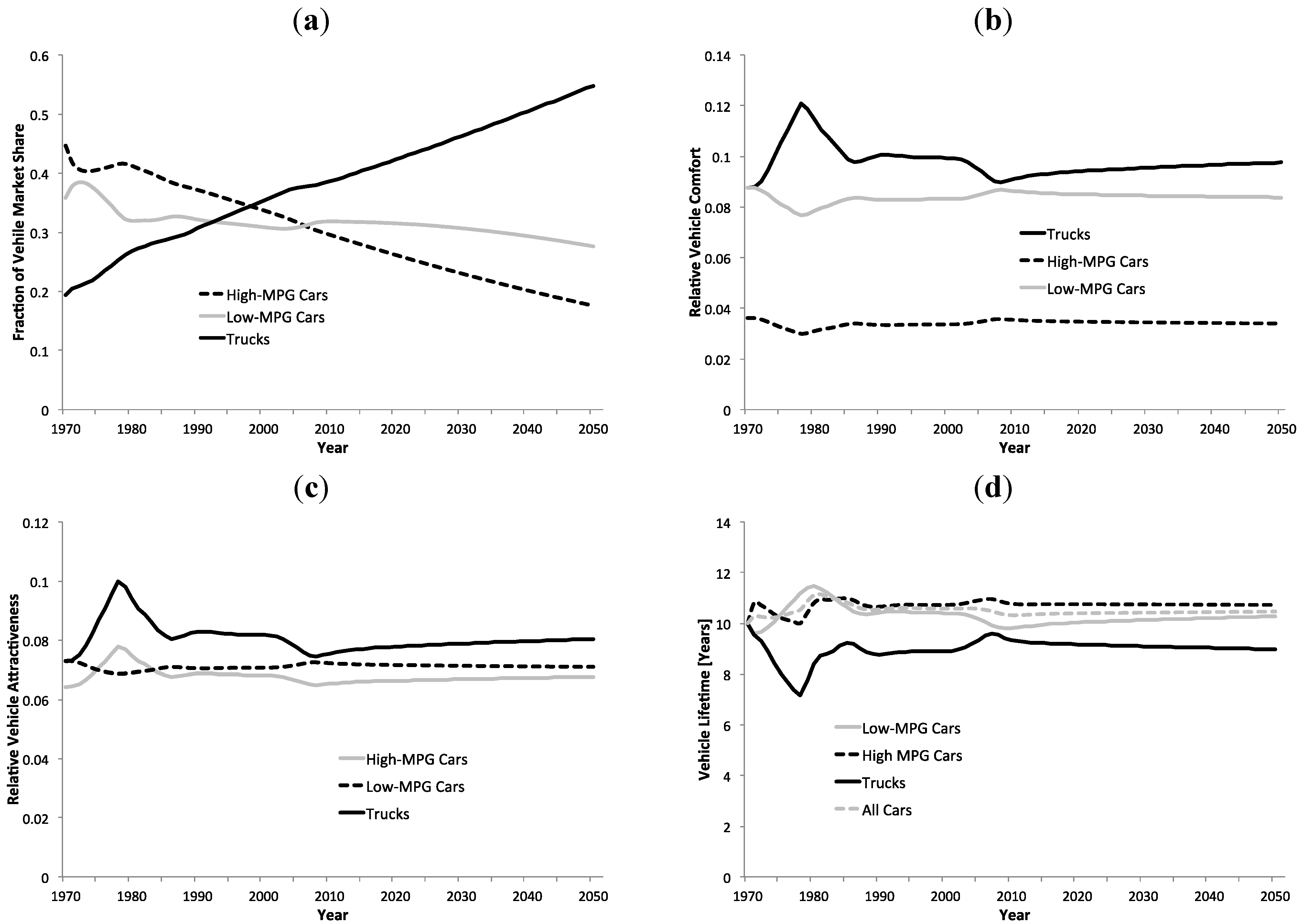
Using these values in the negative logistic growth function, the parameterized model can be tested against a series of real-world datasets for the 1970–2010 period of calibration. These tests, shown in Figure 8 below, demonstrate a reasonable, although not perfect, fit to historical data values.
Figure 8.
Results from Model Calibration. (a) Fit to average fuel economy of new vehicles; (b) Fit to average fuel economy of all vehicles (fleet-wide); (c) Fit to total vehicle miles traveled; (d) Fit to new vehicle market share (high-mpg cars, low-MPG cars, and trucks).
Figure 8.
Results from Model Calibration. (a) Fit to average fuel economy of new vehicles; (b) Fit to average fuel economy of all vehicles (fleet-wide); (c) Fit to total vehicle miles traveled; (d) Fit to new vehicle market share (high-mpg cars, low-MPG cars, and trucks).

5.2. Historical Base Case Run and Future Projections
The historical base case simply allows (1) gasoline price to fluctuate based on historical values (remaining constant from 2010 values onward); (2) CAFE Standards to exhibit historical values after being instituted in 1975 (but they are held constant after the 2011 levels of 30.2 and 24.1 MPG for cars and trucks, respectively); and (3) VMT per year to vary according to gasoline price and slowly ramp due to urban sprawl and the increasing size of the U.S. transportation system. VMT per vehicle approaches 11,500 miles per year by 2008 [53], which reasonably approximates the recent VMT values (2000–2008 avg. = ~11,800; [54]).
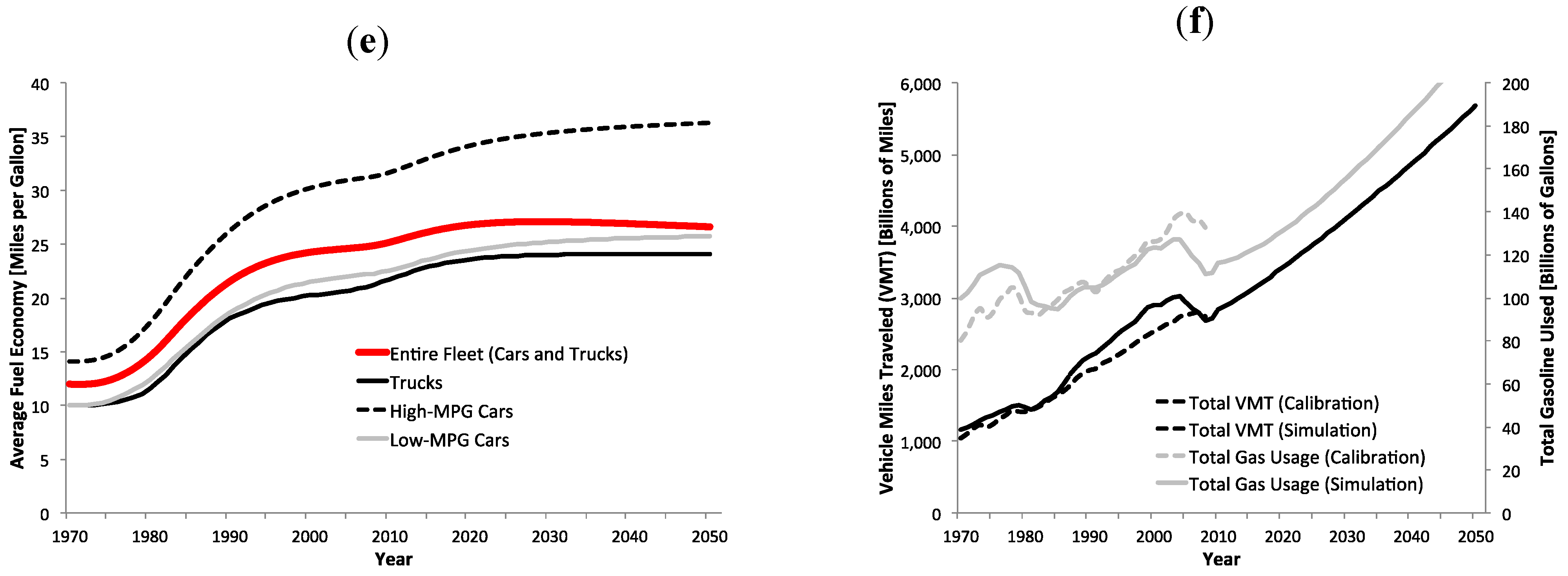
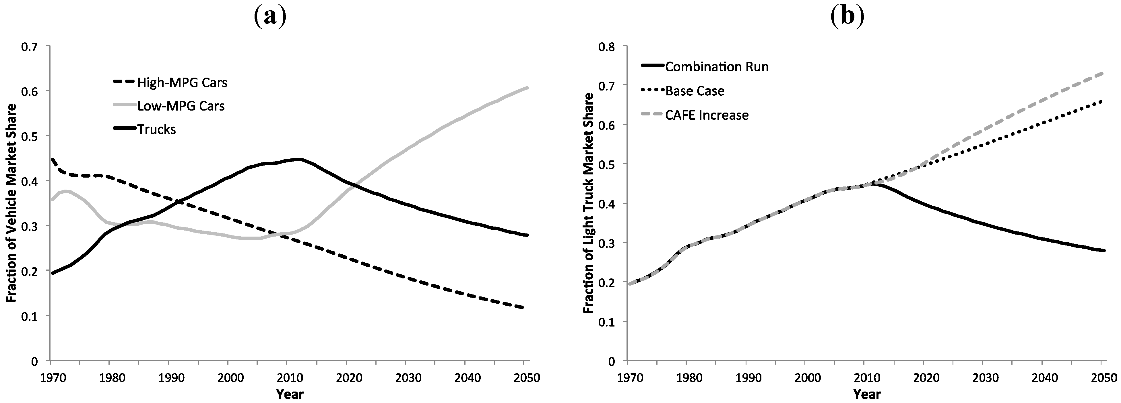
The fraction of high-MPG cars (Figure 9a) decreases in the early 1970s, increases in late 1970s with gas price increases, and then decreases continually as gas prices stay low throughout the 1980s and 1990s. In this simulation, the market share of trucks continues to increase (although the value in 2000 is not as high as the real life value). In 2011, approximately 52% of new vehicle sales were in the truck sector [55]. The model projects a sales figure at roughly 39%. Figure 9b shows the short-term changes in comfort that result from fuel economy and gas price changes, while Figure 9c shows the effects of changing gasoline prices on attractiveness. We see that, after a delay to develop more fuel-efficient vehicles to meet new CAFE standards in the late 1970s, there is a spike in attractiveness in high-MPG cars and trucks to meet demand for more fuel-efficient cars during the period of increased gasoline prices.
Figure 9.
Historical base case run. (a) Market share of new vehicles; (b) Vehicle comfort; (c) Attractiveness of vehicles; (d) Average vehicle lifetime; (e) Vehicle fuel economy; (f) Gasoline usage and vehicle-miles travelled (VMT).
Figure 9.
Historical base case run. (a) Market share of new vehicles; (b) Vehicle comfort; (c) Attractiveness of vehicles; (d) Average vehicle lifetime; (e) Vehicle fuel economy; (f) Gasoline usage and vehicle-miles travelled (VMT).


In Figure 9d we can see the simulated effects of early gasoline price spikes on the average lifetime of vehicles, which mirror the attractiveness spike after the CAFE standards first kicked in and gas prices spiked in the late 1970s. More efficient cars were bought after the gasoline price spike in the late 1970s. When they are retired in the late 1980s when gasoline prices are low, we see a slow shift in market share towards trucks for the next several decades (and low-MPG cars during the 1980s), as exhibited in Figure 9a. It is important to note here that although data exists between 1995 and 2010 on vehicle average age, no consistent data exists that would allow robust calibration of this aspect of the model [56]. As a result, vehicle life simulations have a poor fit to actual data on vehicle life (see Figure 3b). Improving this aspect of the model is a factor that I discuss in recommendations for further research in this article’s conclusions.
The attractiveness of each vehicle type changes in response to both early fluctuations in gasoline prices and gradual decreases in comfort due to increased fuel economy. High-MPG cars (which proxy for small vehicles, as historical data measures) begin as the most common vehicle type, but decrease in market share in the 1970s as relatively attractiveness decreases with falling gasoline prices and shifts in market share towards trucks and low-MPG cars, which remain comparatively far more comfortable.
The average fuel economy of high-MPG cars grows in a goal-seeking pattern from 14.1 MPG to 36.4 MPG, while the fuel economy of low-MPG cars grows from 10.0 MPG to 25.8 during the 70-year simulation (Figure 9b). The average fuel economy of all vehicles rises from 12 MPG to 26.8 MPG, falling from of 27.1 MPG in 2034 as light trucks continue to gain market share. The simulation extrapolates trends seen between 1970 and 2010 in the calibration procedure.
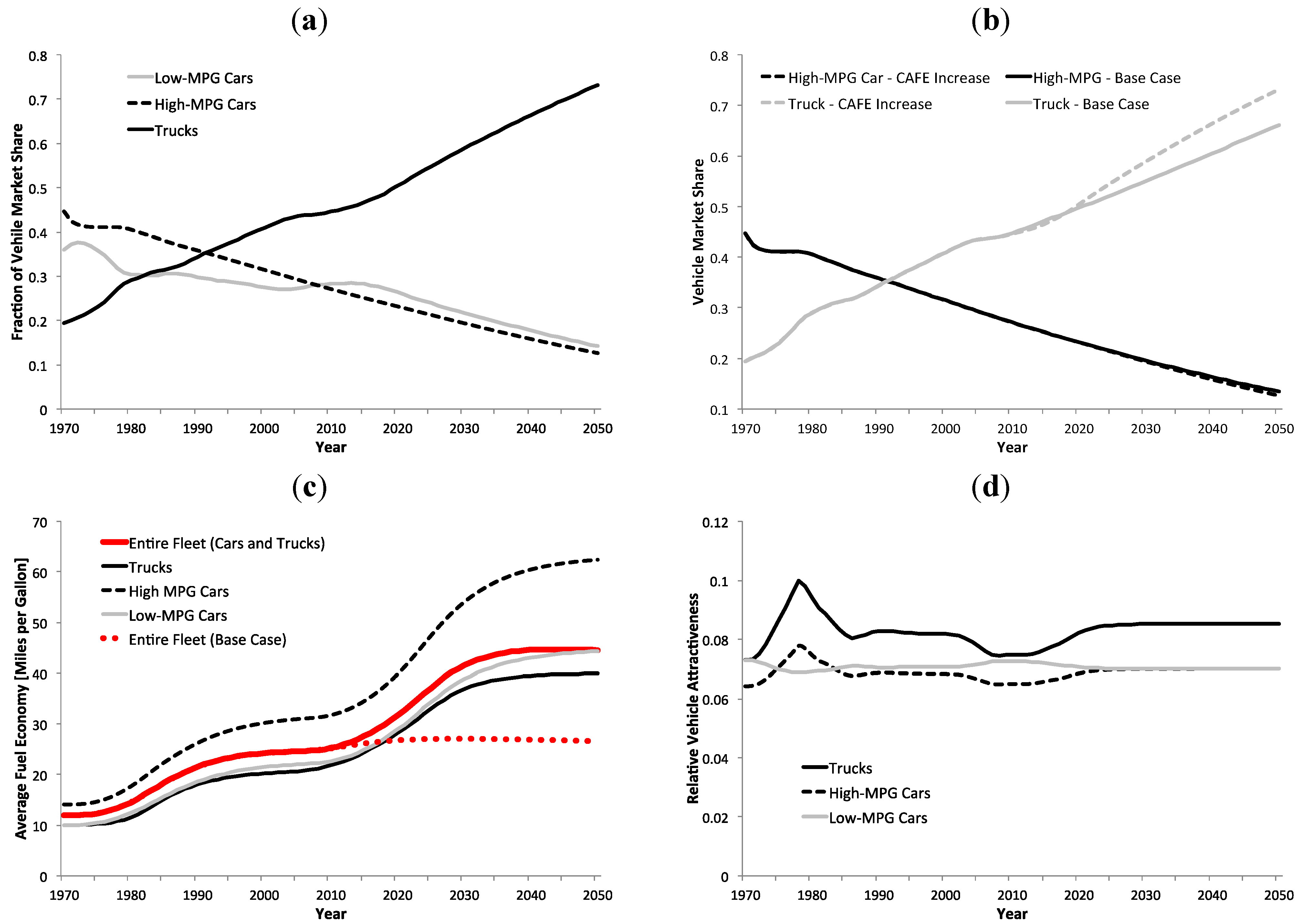
5.3. Imposing Increased CAFE Standards
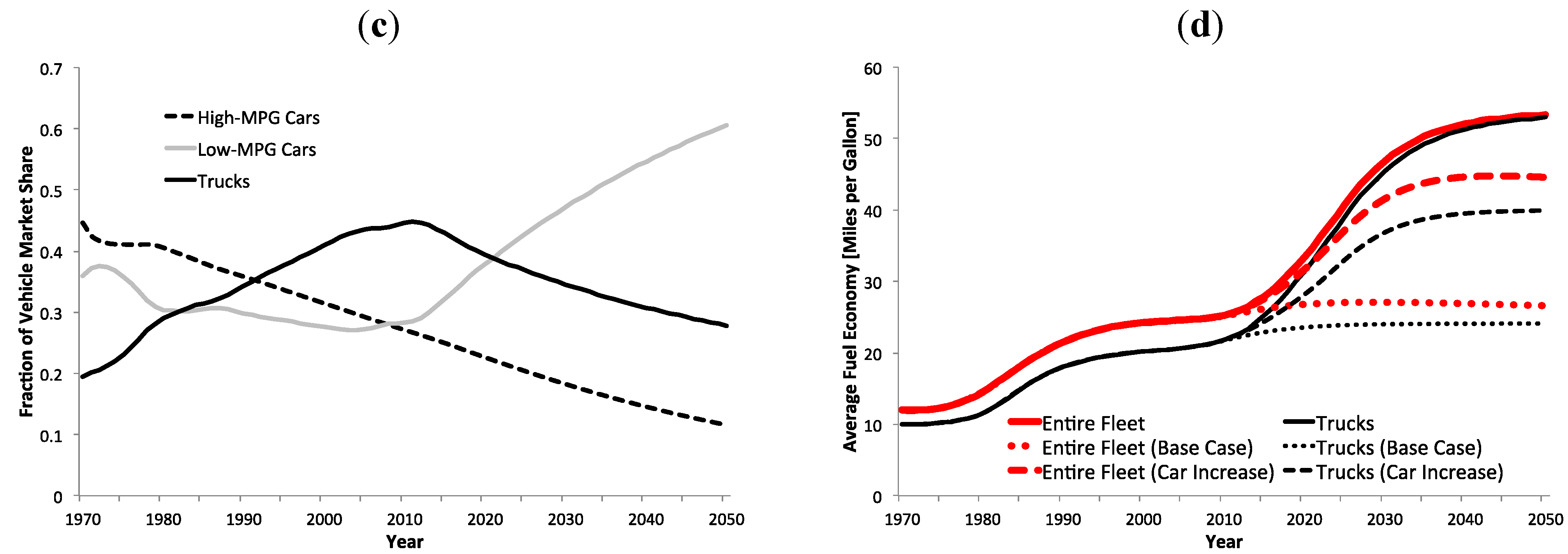
Recent rule making by the NHTSA is intended to dramatically increase CAFE standards over the next 15 years. This run tests the case where CAFE standards are increased from their historical values in the year 2005. This would reflect the behavior of the automobile fleet if car and truck CAFE standards continue to be increased gradually to 2025 to 53.5 MPG and 40 mpg, respectively, as the NHTSA has proposed [17,18].
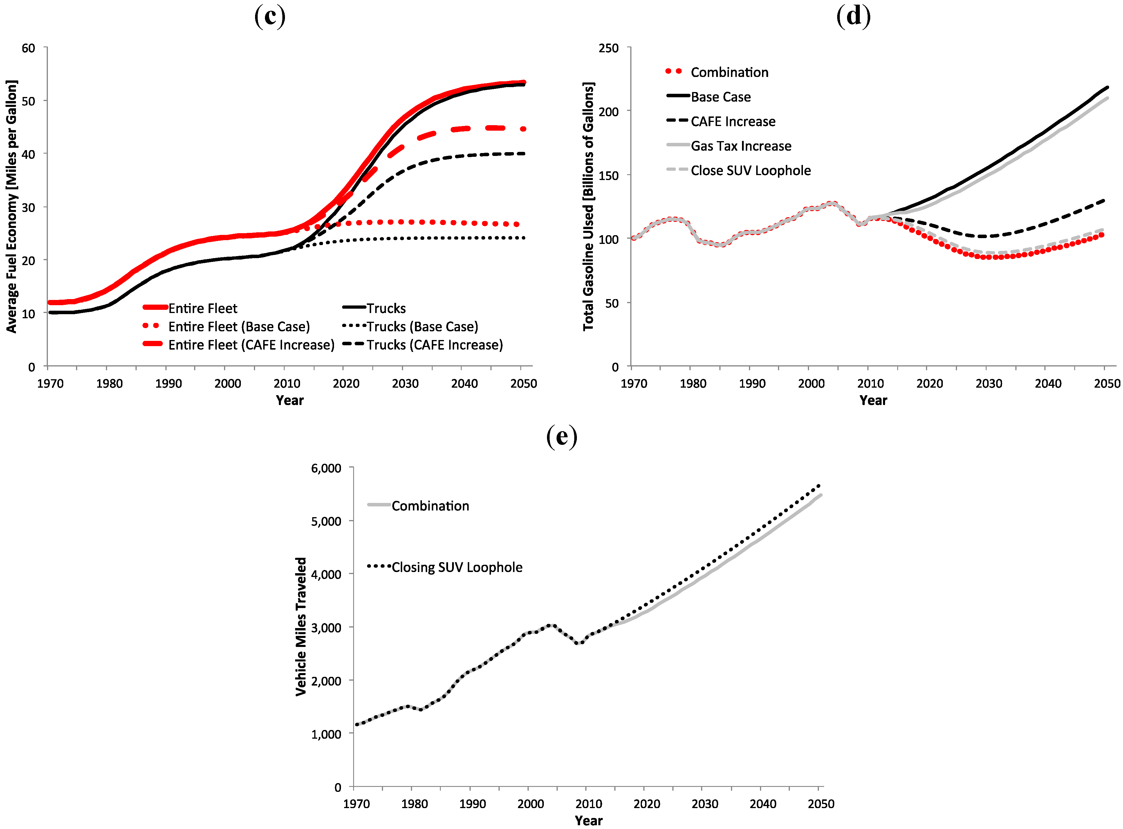
As shown in Figure 10a, the market share of each vehicle type does not change dramatically due to increases in the CAFE standards compared to the base can run in Figure 9a. In fact, market share for trucks actually grows (Figure 10b), as trucks become more attractive due to lower total fuel costs caused by MPG development. The concentration of high-MPG cars in the vehicle fleet stays the same; customers now select vehicles in an environment with even larger discrepancies in required fuel economy standards (Figure 10c), and become even more attracted to increasingly efficient, and comparatively more comfortable, trucks and low-MPG cars (Figure 10d). Because gas prices remain the same, there is little incentive for customers to switch to high-MPG cars.
Increases in fuel economy (Figure 10c) exhibit goal-seeking behavior as manufacturers forecast future CAFE standards (which are planned years ahead of time), and gradually meet these standards over time, thereby exhibiting a first-order smoothing behavior. Unfortunately, although Figure 10e shows that drivers consume less gasoline over the long term due to higher average fuel economy, drivers are more reluctant to purchase the fuel-efficient (high-MPG) cars due to decreased relative attractiveness.
Figure 10.
Simulation of CAFE increases in 2012. (a) Vehicle market shares; (b) Comparison of high-MPG car and truck fractions in base case and CAFE increase scenarios; (c) Comparison of fuel economy of vehicles in base case and CAFE increase scenarios; (d) Vehicle attractiveness; (e) Comparison of total gasoline consumption in base case and CAFE increase scenarios.


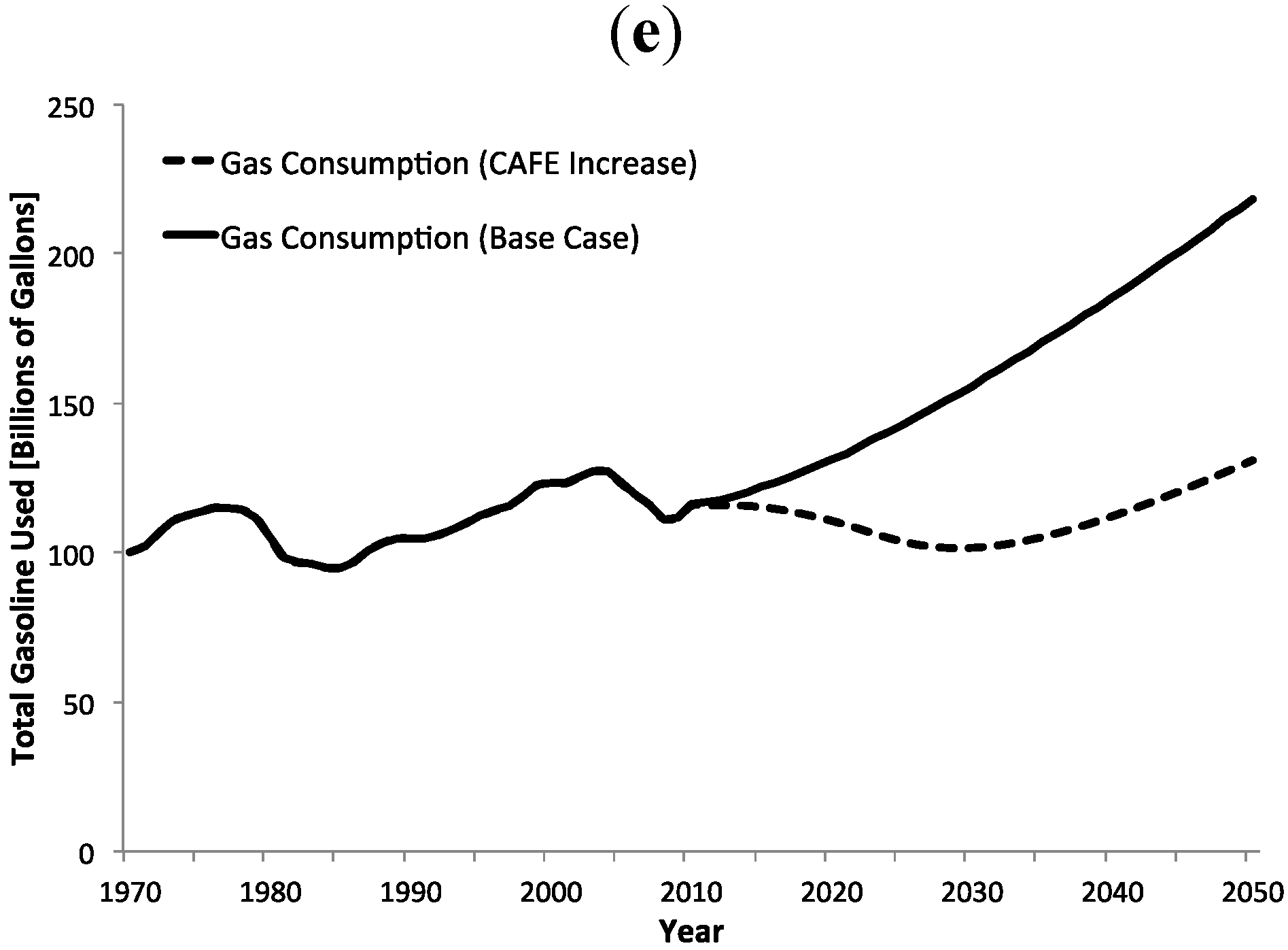
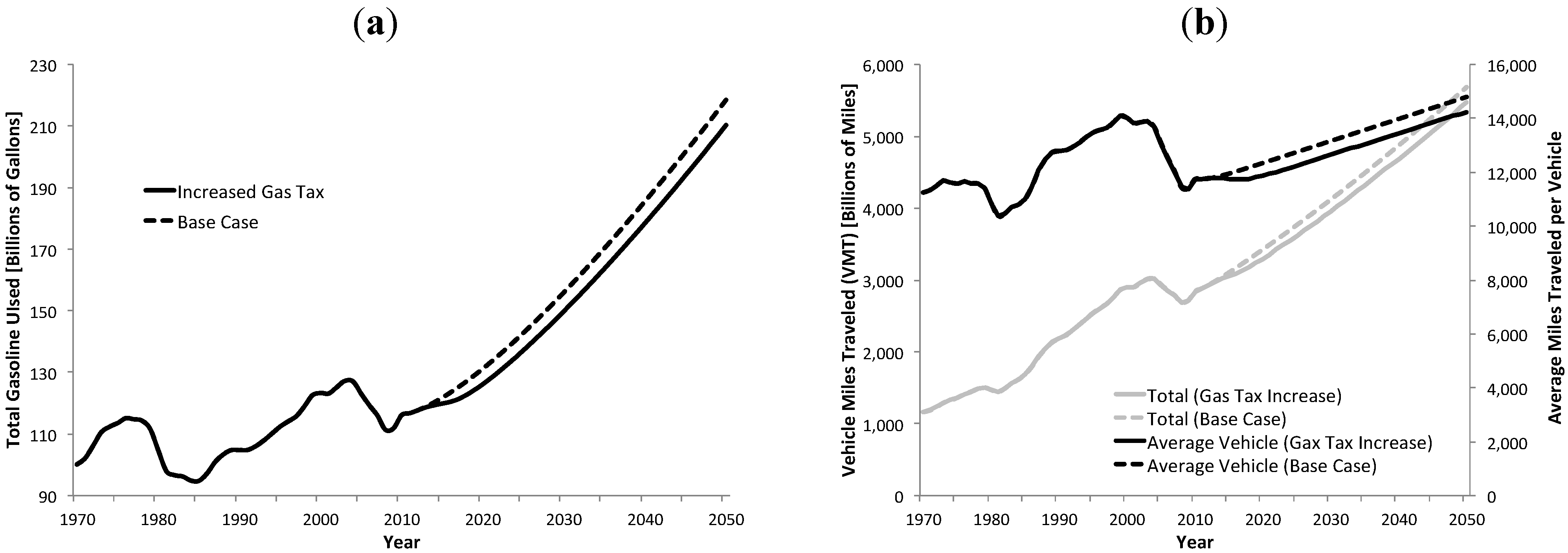
5.4. Imposing a Gasoline Tax
To test the effect of increased gasoline taxes on fleet fuel economy and gasoline conservation, I increase the price of gasoline (via a linear ramp function) to $2.71 a gallon by the year 2020 (CAFE standards remain at their historical values), after which they remain constant until 2050 (all values are taken as the 2005 real values; [57]). A priori, the hypothesis is that vehicle miles traveled are expected to exhibit some change as drivers decrease the amount that they travel.
As I stated before, a major limitation of this model is its inability to capture the feedback between exogenous gas price spikes and the impetus for fuel economy improvements (i.e., MPG increases not mandated under the CAFE standards). As a result, in this simulation, I will look purely at the effect of gas tax increases on the amount driven (VMT) and total gas consumption. In Figure 11a, we can see that, gasoline consumption decreases substantially to compensate for the increased price of fuel; once again, this assumes that regulatory standards are the only mechanism for increasing fuel economy and that manufacturers do not react independently to gasoline increases. In this case, we would expect fuel economy to increase outside of mandated standards, thereby decreasing marginal driving costs and closing any gap in gas consumption or VMT (Figure 11b), as seen in the past [27].
Figure 11.
Gasoline tax increases. (a) Comparison of gasoline consumption in base case and gas tax increase scenarios; (b) Comparison of average and total VMT in base case and gas tax increase scenarios.
Figure 11.
Gasoline tax increases. (a) Comparison of gasoline consumption in base case and gas tax increase scenarios; (b) Comparison of average and total VMT in base case and gas tax increase scenarios.

Interestingly, although consumption levels are decreased relative to the base case, consumption continues to grow despite increases in the gasoline tax. Increases in the gasoline tax do not affect the system’s tendency towards consumption growth (due to population growth and urban infrastructure expansion), but rather decrease the rate at which the growth occurs.
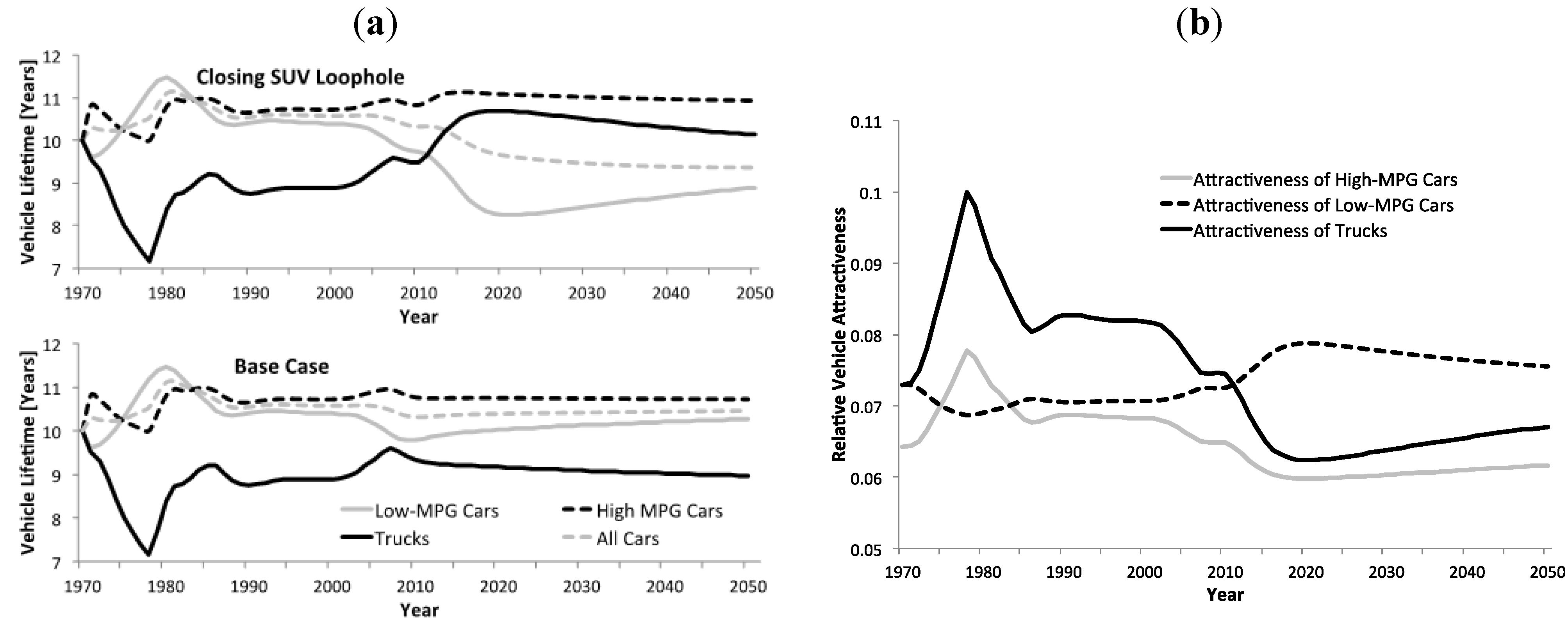
5.5. Closing the SUV Loophole
This policy analysis involves the closing of the “SUV loophole” [15], whereby SUVs and other large vehicles (which have grown dramatically in market share over the last several decades (Figure 3a)), are advantageously characterized as light trucks rather than cars under the CAFE requirements. By requiring SUVs, trucks, and minivans to maintain the same CAFE standard, fuel economy changes would universally affect all vehicles on the road, not just high-MPG cars. This simulation models regulation raising the truck CAFE standard to the same value proposed for cars (53.5 MPG) by 2025.
Figure 12a shows the increase in the life of trucks with increased CAFE standards, as consumers keep their more comfortable, older trucks longer. Figure 12b shows major decreases in truck attractiveness as the CAFE standards are equilibrated, leading to major decreases in truck market share (Figure 12c). Finally, Figure 12d shows the differences in the fleet’s average fuel economy as truck standards are increased, both in comparison to the base case, and in comparison the car-only CAFE standard increases described earlier. In this case, we see the most substantial improvements in average fuel economy of the overall vehicle fleet of any individual policy tested.
Figure 12.
Increased truck CAFE standards to match car standards. (a) Effects on vehicle lifespan; (b) Effects on attractiveness; (c) Comparison of fuel economy of vehicle fleet and trucks in base case and CAFE equivalency scenarios; (d) Vehicle market shares.
Figure 12.
Increased truck CAFE standards to match car standards. (a) Effects on vehicle lifespan; (b) Effects on attractiveness; (c) Comparison of fuel economy of vehicle fleet and trucks in base case and CAFE equivalency scenarios; (d) Vehicle market shares.


5.6. Combined Increases in Gasoline Taxes and CAFE Standards
In the final policy analysis simulation, the previous three tests are combined to determine the effects of concurrent increases in CAFE standards and gasoline price on gasoline consumption and fleet fuel economy. As in the last ‘CAFE equivalency’ test, light truck and car CAFE standards are increased to the same standard of 53.5 MPG by 2025, while gasoline price is raised to $2.71 per gallon by 2016 in the same manner as the test described in the gas tax increase scenario.
Figure 13a shows that, like the previous scenario, low-MPG cars now become the most attractive vehicles on the road. High comfort values and increased fuel economy make this vehicle type very attractive. In Figure 13b, we see light-truck market share declines heavily in comparison to the car-only CAFE increase and the base case scenarios where it previously been dominant. As more drivers seek cars (including the low-MPG cars that now dominate market share), the fleet-wide, average fuel economy will increase towards the ‘final’ CAFE standard of 53.5 MPG; Figure 13c shows this behavior, where fleet-wide average fuel economy begins to increase in 2012.
Figure 13.
Comparison of combination scenario to other scenarios. (a) Vehicle market share; (b) Comparison of truck fractions in base case, CAFE increase, and combination scenarios; (c) Comparison of fuel economy of vehicles and fleet in base case, CAFE increase, and combination scenarios; (d) Comparison of gasoline consumption across all scenarios; (e) Comparison of VMT in combination and ‘closing SUV loophole’ scenario.


Figure 13d compares gasoline consumption for the entire vehicle fleet for all five runs, including the Base Case, car CAFE Increase, Gasoline Tax Increase, Closing the SUV Loophole, and the Combined Policy run. The combined policy of increasing the gasoline tax and CAFE standards concurrently represents the best method of reducing gasoline consumption over the long term. With a relatively small increase in the gasoline tax, increases in CAFE standards, and a closure of the SUV/truck loophole, the fuel economy of the American vehicle fleet increases dramatically. Finally, Figure 13e shows that under the combination scenario, drivers reduce their VMT by 212.75 billion miles per year under that of the SUV loophole closure scenario. Figure 13d, also reveals a 4.042 billion gallon fuel use difference between these two scenarios.
6. Conclusions and Recommendations
The outcomes of these simulations speak directly to the economic environment in which fuel economy policy, consumer behavior, and technological research and development are conducted. This article’s simulations reveal that when increases in mandated fuel economy occur in an economic climate with relatively low fuel costs (relative to income), new vehicle fuel economy increases can easily be counteracted by rapid shifts in tastes of consumers towards larger, more comfortable automobiles.
This is the most pervasive behavior observed in this system. Adjustment to either individual policy ‘lever,’ whether it be isolated changes in CAFE standards or gas prices, can cause policy resistance on the part of the public due to either the lack of incentive to purchase new fuel-efficient automobiles (when CAFE standards are increased), or due to the lack of choices that consumers have of high-MPG vehicles that would assist in reducing the now higher fuel costs (when gas prices are increased). Furthermore, adjustments to CAFE standards alone could incur future rebound effects such as those observed historically [12], whereby higher fuel economy did not lead to decreased overall fuel consumption. However, concurrent adjustment to both policies encourages both reduced VMT and a high turnover rate of older, less fuel-efficient vehicles [58].
The overriding lesson is that gasoline price increases and CAFE regulatory strategies must be employed jointly. As the final simulation shows, a combined strategy will be likely be far more effective than isolated strategies involving mandated CAFE increases or gasoline taxes alone. This combination of polices would provide the incentives necessary to influence consumers and automobile manufacturers to shift towards production of higher efficiency vehicles in ways that minimize welfare losses.
Minimizing welfare losses involves the use of pricing and other regulatory structures for influencing the supply and demand for gasoline together with technology and infrastructure options that expand consumer choice and promote efficiency. For example, a ‘feebate’ approach [59] could be taken, pairing a tax on very inefficient automobiles with subsidies for the development of new, low cost vehicle and energy technologies. This Pigouvian tax would send a dual price signal to manufacturers and consumers that internalizes the social benefits of producing and purchasing high efficiency vehicles [60].
6.1. Recommendations for Further Research
Extensions to this study could include better use of historical data on the weights that consumers place on the different attractiveness attributes associated with the purchase of a new vehicle. Using data such as the APEAL studies by J.D. Power and Associates, which measure the weights that consumers have historically placed on different attractiveness factors when buying a new vehicle, could vastly improve the accuracy of this model. Although collecting this data fell outside the scope of the current study, further research should investigate how these weights are formed and what influences them.
Perhaps the two most important areas of expansion to the model that would add substantial capability involve (1) the introduction of feedback structures that internalize the effects of gas price increases on fuel economy development; and (2) introduction of improved model structures governing the average life of vehicles. Enhancing the model’s ability to accurately replicate effects of CAFE standards and gas prices on vehicle life would be extremely interesting, and would allow further exploration of the effects of changes in either policy. To date, little work has defined direct statistical relationships between vehicle life and CAFE standards.
What happens if an increase in gasoline taxes does not occur in an environment where the new vehicle fleet has improved fuel economy and will entice owners to purchase new vehicles? Will we simply see consumer hesitance towards new vehicle purchases as occurred in the early 1980s [10]? If the marginal cost of driving is high, and consumers can turn to the new vehicle fleet to alleviate that extra cost, vehicle owners might be, at that point, willing to trade in their own vehicles for new, more fuel-efficient trucks. As a result, we might expect to measure vehicle lifespan decreases as consumers are incentivized to purchase new, more fuel-efficient vehicles.
The question for future research on this model becomes, do these policies, in combination, influence American drivers to improve fuel economy without inducing drivers to increase the amount that they drive, thereby decoupling vehicle fuel economy and total gasoline consumption?
Other avenues to improve this model include detailed sensitivity testing and exploration of new model structures that would help to improve model function. For example, sensitivity testing could help better evaluate how the assumptions in this model affect the dynamics connecting attractiveness attributes of vehicle types to their market share, as well as different assumptions about delays in the system. Future explorations of new model structures should look more closely at the relationship between old and new vehicle attractiveness. Creating a more realistic relationship (e.g., assuming that the attractiveness of old vehicles should be a third-order smooth of the average attractiveness of the new vehicle fleet across all vehicle types) could improve the performance of the model, particularly in instances when high-economy cars become highly desirable, yet the retirement rate for trucks and low-economy cars remains low.
These model extensions, coupled with more extensive policy testing, would go towards creating a more accurate and useful model for understanding the effects fuel economy policy and gasoline taxation in the United States.
Acknowledgments
I would like to thank Nikhil Kaza and Jim Lyneis for feedback and advice on drafts of this work, as well as Michael Deegan for his assistance with model calibration. Catherine Raposa assisted with early versions of the model presented in this paper.
Conflict of Interest
The author declares no conflict of interest.
References and Notes
- EIA. EIA Monthly Energy Review. U.S. Energy Information Administration: Washington, D.C., USA, 2011. Available online: http://38.96.246.204/totalenergy/data/monthly/ (accessed on 18 November 2011).
- Robert, K.K.; Stephane, D.; Pavlos, K.; Marcelo, S. Does OPEC Matter? An Econometric Analysis of Oil Prices. Energy J. 2004, 25, 67–90. [Google Scholar]
- Smith, J.L. World Oil: Market or Mayhem? J. Econ. Perspect. 2009, 23, 145–164. [Google Scholar] [CrossRef]
- EIA, Annual Energy Outlook 2011; U.S. Energy Information Administration: Washington, DC, USA, 2011.
- Taylor, J.; Doren, P.V. Don’t Raise CAFE Standards. Abolish them. The National Review: Washington, D.C., 2007. Available online: http://www.nationalreview.com/articles/221732/dont-raise-cafe-standards/jerry-taylor (accessed on 18 November 2011).
- National Highway Traffic Safety Administration (NHTSA). Final Environmental Impact Statement Corporate Average Fuel Economy Standards, Passenger Cars and Light Trucks, Model Years 2011–2015. NHTSA: Washington, DC, USA, 2008. Available online: http://www.nhtsa.gov/fuel-economy (accessed on 20 November 2011).
- Valdes-Dapena, P. Proposed Gas Tax Increase Fires up Debate. CNN-Money: New York, NY, 2010. Available online: http://money.cnn.com/2010/11/11/autos/gas_tax_proposal/index.htm (accessed on 20 November 2011).
- Porter, R.C. Economics at the Wheel: The Cost of Cars and Drivers; Academic Press: San Diego, CA, USA, 1999. [Google Scholar]
- U.S. Federal Trade Commission, Gasoline Price Changes: The Dynamics of Supply, Demand, and Competition; U.S. Federal Trade Commission: Washington, DC, USA, 2005.
- Nivola, P.S.; Crandall, R. The Extra Mile: Rethinking Energy Policy for Automotive Transportation; The Brookings Institution: Washington, DC, USA, 1995. [Google Scholar]
- U.S. Department of Transportation, Bureau of Transportation Statistics (BTS). Multimodal Transportation Indicators. BTS: Washington, DC, USA, 2012. Available online: http://www.bts.gov/publications/key_transportation_indicators/ (accessed on 10 March 2012).
- U.S. Department of Transportation, Federal Highway Administration (FHWA). Quarterly Vehicle Miles of Travel (VMT) 1980–2008. FHWA: Washington, DC, USA, 2011. Available online: http://www.fhwa.dot.gov/policyinformation/charts/07.cfm (accessed on 18 November 2011).
- Energy Policy and Conservation Act of 1975, EPCA, Pub.L. 94-163, 89 Stat. 871, enacted 22 December 1975.
- The EPCA defined “light trucks” to be any truck, minivan, or sports utility vehicle that weighed less than 8,500 pounds.
- Silverman, Z.W. Hybrid vehicles: A practical and effective short-term solution to petroleum dependence. Georgetown Int. Law Rev. 2007, 19, 543. [Google Scholar]
- Energy Independence and Security Act of 2007, EISA, Pub.L. 110-140, originally named the Clean Energy Act of 2007.
- National Highway Traffic Safety Administration (NHTSA). Corporate Average Fuel Economy and CAFE Reform for MY 2008-2011 Light Trucks: Final Regulatory Impact Analysis; NHTSA: Washington, DC, USA, 2006. Available online: http://www.nhtsa.gov/DOT/NHTSA/Rulemaking/Rules/AssociatedFiles/2006_FRIAPublic.pdf (accessed on 25 November 2011).
- National Highway Traffic Safety Administration (NHTSA). 2017–2025 Model Year Light-Duty Vehicle GHG Emissions and CAFE Standards: Supplemental Notice of Intent (40 CFR Parts 85, 86, and 600, 49 CFR Parts 531 and 533); U.S. Environmental Protection Agency and U.S. Department of Transportation: Washington, DC, USA, 2011. Available online: http://www.nhtsa.gov/staticfiles/rulemaking/pdf/cafe/2017-2025_CAFE-GHG_Supplemental_NOI07292011.pdf (accessed on 25 November 2011).
- The International Council on Clean Transportation (ICCT). Global Comparison of Light-Duty Vehicle Fuel Economy/GHG Emissions Standards; ICCT: Washington, DC, USA, 2011. Available online: http://www.theicct.org/sites/default/files/ICCT_PVStd_Aug2011_web.pdf (accessed on 24 April 2012).
- Federal Highway Administration. Highway Statistics 2009 (Table MV-9. Previous years Table VM-1). U.S. Department of Transportation, Federal Highway Administration: Washington, DC, USA, 2011. Available online: http://www.fhwa.dot.gov/policyinformation/statistics/2009/mv9.cfm (accessed on 13 November 2011).
- National Highway Traffic Safety Administration (NHTSA). Summary of Fuel Economy Performance. NHTSA: Washington, DC, USA, 2011. Available online: http://www.nhtsa.gov/fuel-economy (accessed on 19 November 2011).
- U.S. Environmental Protection Agency (EPA), Light-Duty Automotive Technology, Carbon Dioxide Emissions, and Fuel Economy Trends: 1975 Through 2010; EPA-420-R-10-023; Office of Transportation and Air Quality, U.S. Environmental Protection Agency: Washington, DC, USA, 2010.
- Pickrell, D.; Schimek, P. Trends in Personal Motor Vehicle Ownership and Use: Evidence from the Nationwide Personal Transportation Survey; U.S. Department of Transportation Volpe Center: Cambridge, MA, USA, 1998. Available online: http://nhts.ornl.gov/1995/Doc/ Envecon.pdf (accessed on 20 November 2011).
- Polk, R.L. Average Age of Vehicles Reaches Record High. R.L. Polk & Co.: Southfield, MI, USA, 2012. Available online: http://www.polk.com/company/news/average_age_of_vehicles_reaches_record_high_according_to_polk (accessed on 20 March 2012).
- Wards Automotive Group. U.S. Vehicle Sales, 1931-2010 (Key Automotive Data). Wards Automotive: Chicago, IL, USA, 2011. Available online: http://wardsauto.com/keydata/ (accessed on 15 May 2012).
- Bradsher, K. High and Mighty: SUVs—The World’s Most Dangerous Vehicles and How They Got That Way; PublicAffairs: New York, NY, USA, 2002. [Google Scholar]
- Greening, L.A.; Greene, D.L.; Difiglio, C. Energy efficiency and consumption—The rebound effect—A survey. Energy Policy 2000, 28, 389–401. [Google Scholar] [CrossRef]
- Small, K.A.; Dender, K.V. Fuel efficiency and motor vehicle travel: The declining rebound effect. Energy J. 2007, 28, 25–51. [Google Scholar]
- Brozovic, N.; Ando, A.W. Defensive purchasing, the safety (dis)advantage of light trucks, and motor-vehicle policy effectiveness. Transp. Res. Part B: Methodol. 2009, 43, 477–493. [Google Scholar] [CrossRef]
- U.S. Department of Transportation, National Highway Traffic Safety Administration (NHTSA), Relationship of Vehicle Weight to Fatality and Injury Risk in Model Year 1985–93 Passenger Cars and Light Trucks; DOT HS 808 569; NHTSA: Washington, DC, USA, 1997.
- U.S. National Highway Traffic Safety Administration (NHTSA). Vehicle Weight, Fatality Risk and Crash Compatibility of Model Year 1991–99 Passenger Cars and Light Trucks; DOT HS 809 662; NHTSA: Washington, DC, USA, 2003. Available online: http://www.nhtsa.gov/cars/rules/regrev/evaluate/pdf/809662.pdf (accessed on 20 November 2011).
- AIADA. Preserve Consumer Choice By Opposing CAFE Increases. American International Automobile Dealers Association: Alexandria, VA, 2002. Available online: http://web.archive.org/ web/20020306023018/http://www.aiada.org/gr/issues/cafe/cafe.htm Accessed on: 12/3/11.
- Espey, M. Explaining the variation in elasticity estimates of gasoline demand in the United States: A meta-analysis. Energy J. 1996, 17, 49–60. [Google Scholar]
- Goodwin, P.; Dargay, J.; Hanly, M. Elasticities of road traffic and fuel consumption with respect to price and income: A review. Transp. Rev. 2004, 24, 275–292. [Google Scholar]
- Langer, A.; Miller, N.H. Automobile Prices, Gasoline Prices, and Consumer Demand for Fuel Economy; Department of Justice, Antitrust Division: Washington, DC, USA, 2008.
- Although I do not directly model these dynamics, they will be important factors to consider in future work on this topic.
- Cashell, B.; Lazzari, S. Macroeconomic Effects of Increases in the Gasoline Tax. 93-213E; Congressional Research Service: Washington, DC, USA, 1993.
- U.S. Congressional Budget Office (CBO). Economic and Budget Issue Brief: Fuel Economy Standards Versus a Gasoline Tax. CBO: Washington, DC, USA, 2004. Available online: http://www.cbo.gov/doc.cfm?index=5159&type=0 (accessed on 20 November 2011).
- The National Commission on Fiscal Responsibility and Reform. In The Moment of Truth: Report of the National Commission on Fiscal Responsibility and Reform; The White House National Commission on Fiscal Responsibility and Reform: Washington, DC, USA, 2010.
- Sterman, J. Business Dynamics: Systems Thinking and Modeling for a Complex World; Irwin/McGraw-Hill: New York, NY, USA, 2000. [Google Scholar]
- Ford, A. Simulating the controllability of feebates. Syst. Dyn. Rev. 1995, 11, 3–29. [Google Scholar]
- Economy improvements that lower the attractiveness of efficient vehicles would likely lead to market share shifts towards lower-efficiency vehicles. However, automakers must increase the attractiveness of high-MPG vehicles so as to keep the sales-weighted fleet average high enough to comply with CAFE. This dynamic has not been modeled. Although this is an important interaction, the time span for which this model and dynamic hypothesis have been designed cannot accurately represent the monthly changes in car prices that would be needed to account for this situation. Instead, the model assumes that the act of increasing fuel economy through R&D will create a new vehicle fleet that meets the CAFE standards and avoid excessive fines. There is evidence of this dynamic in data on CAFE fines, which show a total of only $800 million fines collected from all automakers between 1978 and 2011.
- U.S. Environmental Protection Agency (EPA), Light-Duty Automotive Technology and Fuel Economy Trends: 1975 Through 2001; EPA420-S-01-001; EPA: Washington, DC, USA, 2001.
- This variable is defined as the following: High-MPG Car Net Fractional Change in MPG = MPG Development Starts − High MPG/MPG of New High MPG Cars Available.
- U.S. Environmental Protection Agency (EPA), Light-Duty Automotive Technology and Fuel Economy Trends: 1975 Through 2005; EPA420-R-05-001; EPA: Washington, DC, USA, 2005.
- National Academies Press (NRC), Assessment of Fuel Economy Technologies for Light-Duty Vehicles; NRC: Washington, DC, USA, 2011.
- The equation governing vehicle attractiveness is used in the same way for all vehicle types. The absolute attractiveness values are normalized for all vehicle types in the New Vehicle Sales Sector.
- Vensim DSS 5.11A Software. Available online: http://www.vensim.com/software.html.
- National Automobile Dealers Association (NADA). NADA DATA: State of the Industry Report 2011; NADA: Mclean, VA, USA, 2011. Available online: http://www.nada.org/NR/rdonlyres/0798BE2A-9291-44BF-A126-0D372FC89B8A/0/NADA_DATA_08222011.pdf (accessed on 20 November 2011).
- The Effect of Lifestyle Changes on VMT is designed to mirror the effects of population increase and broader societal movements in the U.S. (towards lowered urban density) on VMT over time.
- Data, Analysis and Trends: U.S. Light-Duty Fuel Consumption and Vehicle-Miles Traveled (VMT). AFDC: Washington, DC, USA, 2011. Available online: http://www.afdc.energy.gov/afdc/data/vehicles.html (accessed on 3 December 2011).
- Pfaffenbichler, P.; Emberger, G.; Shepherd, S. A system dynamics approach to land use transport interaction modelling: The strategic model MARS and its application. Syst. Dyn. Rev. 2010, 26, 262–282. [Google Scholar]
- The year 2008 was the most recent year of data availability.
- Puentes, R.; Tomer, A. The Road…Less Traveled: An Analysis of Vehicle Miles Traveled Trends in the U.S.; The Brookings Institution, Metrpolitan Policy Program: Washingotn, DC, USA, 2008. [Google Scholar]
- U.S. Department of Energy. Fact #714: February 13, 2012. Light Truck Sales on the Rise. U.S. Department of Energy, Vehicle Technologies Program: Washington, DC, USA, 2012. Available online: http://www1.eere.energy.gov/vehiclesandfuels/facts/2012_fotw714.html (accessed on 11 March 2012).
- Multimodal Transportation Statistics. BTS: Washington, DC, USA, 2012. Available online: http://www.bts.gov/publications/national_transportation_statistics/ (accessed on 18 November 2011).
- Although recent (2012) gas prices are much higher, it is important to note that between 1970 and 2010, the average (inflation adjusted) price of gasoline was $1.82 (2005$). Therefore, an increase of gas prices to $2.71 (15 cents over the 2010 average price of $2.56) is actually quite expensive compared to historical values.
- In the gas tax increase and combination policy scenarios, average VMT continues to climb despite the higher price of gasoline. Testing on this variable reveals sensitivity issues; VMT increases most likely would not occur in an environment where gas prices had just doubled. The formulation for VMT in this model includes a ramp function that works independently of gasoline price and mimics an increasing population of vehicle owners. If gasoline prices doubled, there might also be more reluctance for future vehicle owners to actually purchase a car. That being said, in this situation, intuition suggests that overall VMT should decline. In addition to this, if gasoline prices doubled, current vehicle owners would most likely limit their leisure drives and other unnecessary trips. While this feedback is indeed formulated in this model, the VMT equations are not sensitive enough to result in an adequate reduction in VMT for larger gas tax scenarios.
- BenDor, T.; Ford, A. Simulating a combination of feebates and scrappage incentives to reduce automobile emissions. Energy 2006, 31, 1197–1214. [Google Scholar]
- Sperling, D. Future Drive: Electric Vehicles and Sustainable Transportation; Island Press: Washington, DC, USA, 1995. [Google Scholar]
© 2012 by the authors; licensee MDPI, Basel, Switzerland. This article is an open-access article distributed under the terms and conditions of the Creative Commons Attribution license (http://creativecommons.org/licenses/by/3.0/).
Share and Cite
MDPI and ACS Style
BenDor, T.K. The System Dynamics of U.S. Automobile Fuel Economy. Sustainability 2012, 4, 1013-1042. https://0-doi-org.brum.beds.ac.uk/10.3390/su4051013
AMA Style
BenDor TK. The System Dynamics of U.S. Automobile Fuel Economy. Sustainability. 2012; 4(5):1013-1042. https://0-doi-org.brum.beds.ac.uk/10.3390/su4051013
Chicago/Turabian StyleBenDor, Todd K. 2012. "The System Dynamics of U.S. Automobile Fuel Economy" Sustainability 4, no. 5: 1013-1042. https://0-doi-org.brum.beds.ac.uk/10.3390/su4051013