Multi-Temporal Patterns of Urban Heat Island as Response to Economic Growth Management

Abstract

For a reliable assessment of sustainability in big cities, it is imperative to evaluate urban ecosystem conditions and the environment of the cities undergoing economic growth. Urban green spaces are valuable sources of evapotranspiration, which is generated by trees and vegetation; these spaces mitigate urban heat islands in cities. Land surface temperature (LST) is closely related to the distribution of land-use and land-cover characteristics and can be used as an indicator of urban environment conditions and development. This study evaluates the patterns of LST distribution through time by employing the thermal spatial distribution signature procedure using thermal infrared data obtained from Landsat-5 Thematic Mapper. A set of 18 images, between 1985 and 2010, was used to study the urban environment during summer in 47 neighborhoods of Porto Alegre, Brazil. On a neighborhood scale, results show a non-linear inverse correlation (R² = 0.55) between vegetation index and LST. The overall average of the LST is 300.23 K (27.8 °C) with a standard deviation of 1.25 K and the maximum average difference of 2.83 K between neighborhoods. Results show that the Thermal Spatial Distribution Signature (TSDS) analysis can help multi-temporal studies for the evaluation of UHI through time.

1. Introduction

Owing to civilization in the 19th century, land use cover was strongly transformed without precedent, which is strongly related to the high acceleration of industrialization. In recent decades, excessive local demands on environmental systems have become global in scope [1]. Since then, soil occupation processes have been frequently demonstrated to be in disagreement with sustainable development concepts. Although there are a number of diverse definitions of urban sustainability, the core value of urban sustainability always lies in the balance of environmental, economic and social development [2,3]. However, the monitoring of local environmental problems and planning has been increasingly perceived as an institutional and governmental tool for introducing principles of sustainable development as well as for serving as urban sustainability indicators [2]. Herein, environmental problems refer to any human-induced damage to the physical environment resulting from land use and land cover (LULC), estate pressure, inadequate waste management and unintended side effects caused by human activity in the urban environment.

Surface and atmospheric modifications caused by urbanization generally lead to a modified thermal climate, which is warmer than the surrounding non-urbanized areas [4]. Cities use construction materials, such as concrete and asphalt, which do not allow water to penetrate into the soil. In addition, a high proportion of the incident shortwave radiation is absorbed and transformed into sensible heat [5]. This phenomenon, which modulates the air temperature of the lowest layers in the urban atmosphere, is called urban heat island (UHI); it is central to the surface energy balance, it helps to determine the internal climate of buildings and it affects the energy exchanges that affect the comfort of city dwellers [4].

It is essential to have knowledge about UHI in earth sciences for urban climatology, global environmental change and management practices in the urban environment because Land Surface Temperature (LST) is closely related to the distribution of LULC characteristics [6,7], and the physical conditions and properties of the vegetation types and surrounding urban environment are key factors that determine LST distribution [8].

It is well known that shade trees and even small plants for land cover, such as shrubs and grass, help cool the urban environment [9]. Green space or vegetation areas are, in an absolute sense, an indispensable component of urban sustainability [2]. Several benefits can be ascribed to green spaces in the urban environment caused by their capacity of cooling the air [10] and reducing the available surfaces for successively radiating energy reflectance. Furthermore, urban green spaces are always beneficial, not only for mitigating UHI, but also for evapotranspiration, which is generated by trees and vegetation in cities, and for cooling the air by using the surrounding urban environment heat from the air to evaporate water [11].

A literature review has indicated that thermal satellites with adequate temporal and spatial resolution data can accurately estimate surface physical properties and other related variables [12,13,14,15,16,17]. Study from [18] has demonstrated that urban areas could be studied and identified by means analyses of thermal remote sensing data.

Most of the research has focused on the classification accuracy of features and mapping. However, there has been significantly less interest in the development of methods that concentrate on the understanding of statistical implications on the classification of the temporal resolution of features and LULC through time.

The Landsat data series satellites have collected several years of data in the thermal spectral band and have been used in several studies on UHI [19]. For the reliable assessment of sustainability in big cities, it is imperative to evaluate urban ecosystem conditions and the environment for cities undergoing economic growth. Thus, the launch of the Landsat Data Continuity Mission (LDCM) on 11 February 2013, which carried the thermal infrared sensor (TIRS), will extend the Landsat data archive from the earlier missions, thereby allowing long-term studies [20].

In this study, we discuss the development of a quantitative methodology for the evaluation of the general physical conditions of the urban environment based on the vegetated land cover characteristics by monitoring of the LST distribution in the urban environment. Multi-temporal imagery analysis is essential to UHI studies [21]. We also evaluate a specific approach for the identification of multi-temporal patterns of LST distribution in the urban environment.

The concept for the assessment of urban LST distribution is referred to as thermal spatial distribution signature (TSDS) from the study of [18]. This paper takes their method a step further and combines the applicability of medium spatial resolution satellite imagery and provides an objective methodology for decision makers and planners. In this paper, we do not evaluate the absolute temperature fluctuations in different periods. Instead, we evaluate the increase of separability between temperatures of neighborhoods after several years of urban environment development. The objective is to develop an LST-based procedure using medium-resolution sensor images, which can aid in the understanding of urban environment development and land cover change assessment.

2. Materials and Methods

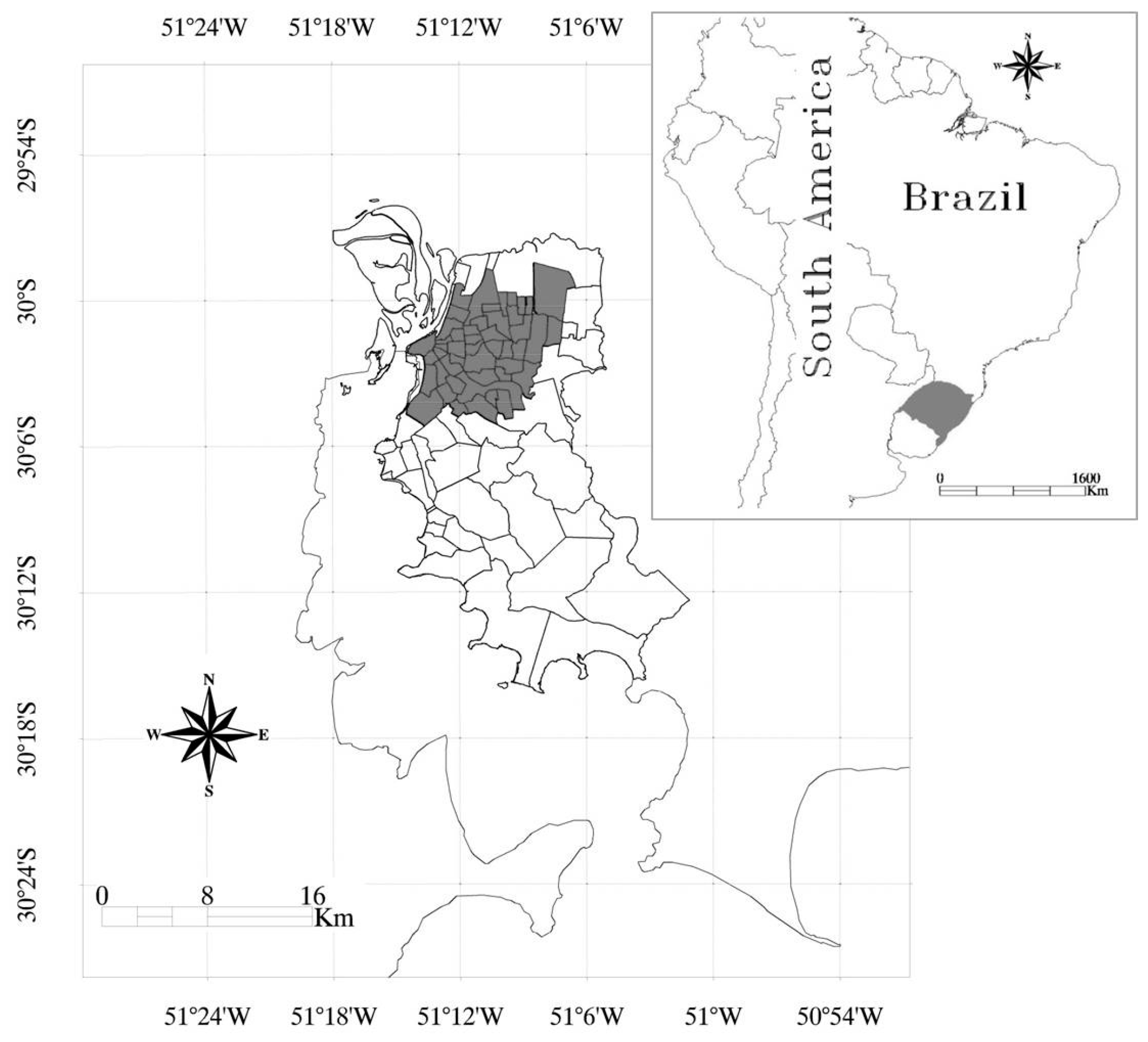
2.1. Study Area

The study area is the city of Porto Alegre, located at latitude of 30°01′59′′ South and longitude of 51º13′48′′ West. The region predominantly experiences a subtropical mid-latitude climate (Cfb) with four well-defined seasons [22]. The mean annual temperature is 19.5 °C, varying between 12 ºC and 26 °C. The monthly mean precipitation is 114 mm, and the yearly-accumulated average precipitation is 1373 mm with no dry period. The city is covered by a Landsat scene path 221/row 081. The municipality elevation average is 19 m above the sea level, with the total population of the city being 1,467,816 in 2013 [23]. This study analyzes 47 neighborhoods near downtown, which covers an area of 9077 ha. Neighborhoods are distributed alongside the downtown from west side to east side towards rural areas. Figure 1 shows the study area.

Figure 1. Urban area of Porto Alegre in Brazil and the study area with 47 neighborhoods.

Figure 1. Urban area of Porto Alegre in Brazil and the study area with 47 neighborhoods.

2.2. Satellite Imagery and Data Set

Our analysis combined Landsat-5 TM images from different periods. A set of 25 images was initially used to study vegetation conditions and the development of the urban environment between 1985 and 2010; however, only 18 images were specially selected because of better atmospheric conditions.

To evaluate the most precise combination data for multi-temporal analysis, the key question is what are the window periods and their extension for performing adequate imagery combination and for extracting LULC diagnosis. By using this conceptual question, the TSDS procedure consists of the analysis and interpretation of statistical data associated with LULC, which leads to the spatial and temporal variations of LST distribution. In this study, the data sources used for TSDS distribution analysis included the following information levels:

• Monthly rainfall data obtained from the Database for Meteorological Research of the Instituto Nacional de Meteorologia [24], which covers the period from October to December. These data were used to identify drought periods in the warmest season;
• Climatological normal of accumulated rainfall from October to December;
• Landsat-5 TM images distributed in Brazil by the Instituto Nacional de Pesquisas Espaciais [25];
• Digital geospatial reference from National Aeronautics and Space Administration-Global Land Survey [26].

2.3. Imagery Calibration and Data Generation

2.3.1. Reflectance Data Generation

Reflectance values were generated by complete calibration and correction of digital numbers (DN) according to Landsat Calibration Documents [27]. After conversion to at-satellite radiance, each image was converted to at-satellite reflectance (assuming a uniform Lambertian surface under cloudless conditions). First, in this study, DN were converted into radiance and next to reflectance, according to the calibration parameters of [28] and LST [29] at the same math code. Regarding the calibration of reflectance channels, for the accurate transformation of DN into reflectance data, the images were also atmospherically corrected according to [30], as variations of atmospheric conditions are spatially and temporally significant [27]. Correction includes atmospheric- and sensor-related parameters and then the derivation of physical units, such as reflectance [31]. In the strict sense, full image correction involves both applications of absolute calibration coefficients for sensors and parameters related to atmospheric correction to derive surface reflectance estimates [27]. By this approach, the data necessary to perform atmospheric correction in the visible bands 1–5 can be obtained from the image itself [32] by restricting the atmospheric influence, as the radiation transfer from the Earth’s surface to on-orbit sensors causes a weighted displacement effect, which depends on the wavelength of visible bands on a per-pixel-basis demand. Considering the imagery processing protocol established in [17] as a quality control for the atmosphere effect, Landsat 5 TM imagery was submitted to a threshold criterion to which no image was used when the amount of atmospheric contamination effects exceeded 60 DN in the blue band.

TOA reflectance can be obtained by applying the radiance–reflectance conversion equation, according to Equation (1).

$$\text{ρ}=\frac{{\text{π L}}_{\text{λ }}{\text{d}}^2}{{\text{ESUN}}_{\text{λ }}{\text{cosθ}}_{\text{s}}}$$

(1)

Where,

• L_λ is the spectral radiance at the sensor in each band (W m⁻² sr⁻¹μm⁻¹);
• d is the distance between the Earth and the Sun in astronomic units (UA);
• ESUN_λ is the average solar atmospheric irradiance (W m⁻² μm⁻¹); and
• θ_s is the solar zenith angle (degrees).

Reflectance values from bands 3 and 4 were used to generate the enhanced vegetation index (EVI-2) data according to Equation (2) from [33]. EVI-2 is a two-band version of EVI that has been developed for sensors without a blue band [33]. It retains sensitivity and linearity as EVI for high leaf area index (LAI) canopies but does not rely on the usually poor-quality blue band [34]. Once we have the corrected TOA reflectance, EVI-2 can be computed without a blue band but remains equivalent to EVI. In this way, EVI-2 calculation (Equation (2)) can be used as an acceptable substitute of EVI over atmospherically corrected pixels [33]. NIR and Red represent the obtained reflectance in the near-infrared and red bands of Landsat-5 TM, respectively.

$$\text{EVI}2=2.5\frac{\text{NIR}-\text{Red}}{\text{NIR}+2.4\text{ Red}+1}$$

(2)

2.3.2. Thermal Data Generation

For thermal analysis, from band 6, after converting DN into absolute radiance values, LST is computed from at-satellite brightness temperatures (i.e., blackbody temperature) under the assumption of unity emissivity and using pre-launch calibration constants [27,35]. Then, LST is corrected to non-unity surface emissivity according to the formulation from [29], which does not perform corrections to atmospheric effects (absorption and emissions along the path) because of the difficulty with estimating water vapor content from thermal detection in the mono-window band 6 [36,37].

The conversion of the detected thermal radiation to brightness temperature [27] is given in Equation (3), which is a special case of Plank’s radiating law. Numerous factors need to be quantified to assess accurate LST retrieval from satellite thermal data, including sensor radiometric calibration [38], atmospheric correction [30,39], surface emissivity correction [40] and physically driven conditions of land coverage [7]. Next, LST is obtained by correcting the radiating surface temperature to the surface emissivity (ε), which is the ratio of the thermal energy radiated by the surface to the thermal energy radiated by a blackbody at the same temperature [40]. The accurate retrieval of LST from thermal spectral bands also requires an estimate of emissivity from surface coverage [41]. Surface emissivity is controlled by factors, such as water content, chemical composition, structure and roughness [42]. Emissivity depends on the LAI as given by Equation (4) [40] as follows:

$$\text{LST}=\frac{\text{K}2}{\text{ln}\left(\frac{{\text{ε}}_{\text{NB}}\text{K}1}{\text{L}}+1\right)}$$

(3)

$${\text{ε}}_{\text{NB}}=0.97+0.0033\text{ LAI}$$

(4)

where,

• LST is the emissivity-corrected surface temperature (K);
• K1 is the calibration constant 1 (607.76 W m⁻² sr⁻¹μm⁻¹);
• K2 is the calibration constant 2 (1260.56 W m⁻² sr⁻¹μm⁻¹);
• L is the blackbody radiance of the thermal band 6 (W m⁻² sr⁻¹μm⁻¹); and

εNB is the emissivity factor, which depends on the type of surface coverage conditions when LAI < 3.0, εNB = 0.98 because the increased water content in vegetation actually increases emissivity capacity.

The generated image product is composed of cloud-free images and good-quality geo-referencing metrics. The latter was used to provide accurate geo-registration on a per-pixel-basis of the selected images, as shown in Table 1.

Table 1. Selected Landsat-5 TM imagery for monitoring the studied area.

Imagery		Land Surface Temperature (LST)				Enhanced Vegetation Index (EVI-2)
	Date	Min.	Max.	Average	SD	Min.	Max.	Average	SD
1	05 Jan. 1985	291.3	303.5	298.6	1.22	−0.19	0.51	0.09	0.100
2	06 Feb. 1985	292.2	304.4	298.7	1.45	−0.27	0.53	0.11	0.113
3	24 Jan. 1986	298.6	310.8	305.4	1.51	−0.27	0.52	0.11	0.113
4	20 Feb. 1990	289.4	302.7	297.7	1.77	−0.32	0.54	0.11	0.119
5	06 Jan. 1991	296.2	319.3	305.1	1.83	−0.28	0.53	0.11	0.117
6	09 Jan. 1992	293.8	304.0	299.6	1.24	−0.23	0.53	0.10	0.107
7	12 Feb. 1993	292.2	302.7	297.9	1.32	−0.21	0.54	0.11	0.116
8	30 Jan. 1994	296.0	307.6	302.3	1.42	−0.30	0.52	0.11	0.116
9	06 Jan. 1997	293.8	305.6	299.7	1.46	−0.16	0.52	0.10	0.110
10	27 Dec. 1998	292.9	305.6	300.5	1.63	−0.55	0.68	0.09	0.110
11	02 Feb. 2001	291.5	303.1	297.4	1.28	−0.25	0.52	0.09	0.110
12	20 Jan. 2002	294.0	304.0	299.6	1.16	−0.24	0.51	0.09	0.105
13	11 Feb. 2004	289.9	304.4	298.1	1.50	−0.37	0.51	0.09	0.107
14	12 Jan. 2005	287.5	313.6	305.2	2.02	−0.35	0.49	0.08	0.096
15	02 Jan. 2007	294.9	307.6	301.7	1.68	−0.32	0.52	0.10	0.113
16	06 Feb. 2008	290.4	305.2	298.3	1.75	−0.27	0.54	0.10	0.110
17	07 Jan. 2009	289.4	303.1	296.5	1.76	−0.25	0.51	0.10	0.116
18	28 Dec. 2010	293.1	309.3	301.7	2.17	−0.39	0.51	0.10	0.113

Note: SD: Standard Deviation.

Table 1. Selected Landsat-5 TM imagery for monitoring the studied area.

Imagery		Land Surface Temperature (LST)				Enhanced Vegetation Index (EVI-2)
	Date	Min.	Max.	Average	SD	Min.	Max.	Average	SD
1	05 Jan. 1985	291.3	303.5	298.6	1.22	−0.19	0.51	0.09	0.100
2	06 Feb. 1985	292.2	304.4	298.7	1.45	−0.27	0.53	0.11	0.113
3	24 Jan. 1986	298.6	310.8	305.4	1.51	−0.27	0.52	0.11	0.113
4	20 Feb. 1990	289.4	302.7	297.7	1.77	−0.32	0.54	0.11	0.119
5	06 Jan. 1991	296.2	319.3	305.1	1.83	−0.28	0.53	0.11	0.117
6	09 Jan. 1992	293.8	304.0	299.6	1.24	−0.23	0.53	0.10	0.107
7	12 Feb. 1993	292.2	302.7	297.9	1.32	−0.21	0.54	0.11	0.116
8	30 Jan. 1994	296.0	307.6	302.3	1.42	−0.30	0.52	0.11	0.116
9	06 Jan. 1997	293.8	305.6	299.7	1.46	−0.16	0.52	0.10	0.110
10	27 Dec. 1998	292.9	305.6	300.5	1.63	−0.55	0.68	0.09	0.110
11	02 Feb. 2001	291.5	303.1	297.4	1.28	−0.25	0.52	0.09	0.110
12	20 Jan. 2002	294.0	304.0	299.6	1.16	−0.24	0.51	0.09	0.105
13	11 Feb. 2004	289.9	304.4	298.1	1.50	−0.37	0.51	0.09	0.107
14	12 Jan. 2005	287.5	313.6	305.2	2.02	−0.35	0.49	0.08	0.096
15	02 Jan. 2007	294.9	307.6	301.7	1.68	−0.32	0.52	0.10	0.113
16	06 Feb. 2008	290.4	305.2	298.3	1.75	−0.27	0.54	0.10	0.110
17	07 Jan. 2009	289.4	303.1	296.5	1.76	−0.25	0.51	0.10	0.116
18	28 Dec. 2010	293.1	309.3	301.7	2.17	−0.39	0.51	0.10	0.113

Note: SD: Standard Deviation.

2.4. LST and Biophysical Descriptors

In the natural environment, dry, bare and low-density soils, for example, have been linked to high LST as a result of the relatively low thermal inertia [43]. These thermal properties vary with the type of soil and moisture content [43]. On the other hand, in the urban environment, non-evaporative and impervious surface areas not only play an important role in UHI formation [14] but also in heat generated by anthropogenic sources, such as traffic and industries [44]. This is because the emissivity of soils or sparsely vegetated areas is a function of soil moisture conditions and soil density [17,41,44,45]. The physical fundamentals for such a relation rely on the fact that for any surface material, certain internal properties, such as heat capacity, thermal conductivity and inertia, play important roles in governing the temperature of a body at equilibrium with its surroundings [46].

Leaves and branches reduce the amount of solar radiation that reaches the area below the canopy of a tree or plant reducing the energy to be converted to heat on the surface. In the summer season, generally 10%–30% of the Sun’s energy reaches the area below a tree, with most of it being absorbed by leaves and used for photosynthesis and some being reflected back into the atmosphere [9]. Even so, thermal responses for vegetation can also vary highly as a function of the biophysical properties of the vegetation itself as well [6,47]. This concept is based on the assumption that vegetation coverage mitigates high LST occurrence values. The relationship between thermal characteristics of surface and vegetation indices has been extensively documented in the literature [7,13,48,49,50,51,52]. Many studies have observed a negative relationship between LST and vegetation indices. Given this and considering that temperature is closely related to physiological activities of vegetation cover, LST can be a useful measure of the physiological activity of the top canopy leaves when a leaf cover is sufficiently high such that they are not affected by background temperature from soil [50].

For UHI studies, the LST and vegetation index relationship has been utilized by several authors [19,53] to understand the role of LST in urban development and vegetation coverage dynamic assessment. The LST obtained from satellite imagery is, strictly speaking, a measure of the “skin temperature” or surface radiometric energy (kinetic) emitted from the land surface and is related to the thermal infrared (TIR) radiation rather than air temperature [36,41], which is more commonly used in physiological studies [50].

In surface areas characterized by full vegetated or fraction of vegetation cover, thermal properties from non-vegetated surface areas can significantly influence the surrounding measurements of LST through the thermal processes related to direct sunlight interception. In this way, when studying a histogram of LST distribution through time, it is expected that the highly developed and urbanized areas or sparsely vegetated areas are unable to cool the surrounding sensible heat by evapotranspiration, as it typically does, which leads to a spread of LST range by increasing statistical indicators in terms of the variance of distribution towards higher LST values. However, vegetation index measurements are subject to seasonal variations, which may influence the results on UHI studies, and thus, such measurements may not serve as a good indicator for urban development [44].

2.5. TSDS Approach

The study of LST is closely related to the distribution of LULC characteristics. Typically, simplified models that describe LULC can provide a link between LST and physical spatial distribution. However, LST is highly variable through time, which does not allow the comparison of absolute values in a simplified conceptual approach. In addition, further statistical analysis plays an important role in linking LST to the surface characteristics [47]. In doing so, to better understand the physical descriptors of heating effects over the urban environment, as a representative of their development through time, we only compared the summer season imagery from late December to February, in order to detect the most pronounced LST values associated with surface coverage.

The TSDS procedure using TIR data obtained from Landsat-5 TM was applied to evaluate the radiometric pattern of the urban environment and vegetation coverage conditions. TSDS is a criterion for multi-temporal imagery combination of data, which is based on the relation between the thermal characteristics of surface and coverage and consists of the standard deviation (SD) analysis of LST to compare images by means similarity characteristics. This is because during some periods, intensive cover change caused by seasonal conditions or even different government policies can cause a rapid urban environment change in relatively few years.

By using the TSDS approach over the urban environment, it is possible to observe variations in the LULC area through time, and after that, to stabilize groups of similar imagery data according to their spatial distribution conditions. Furthermore, regarding the relation between LST and vegetation index, and considering the same study area through time, heterogeneous surface coverage with different types of impervious surface coverage presents a range of temperature distribution wider than that where homogeneous green areas prevail [44].

It is important to note that the studied urban area in the early period (1980s) was under physically driven conditions of surface and vegetation coverage different from those in the most recent period. The main problem for an individual analysis of the imagery data set is associated with the high variability related to urban environment dynamics [35] and seasonality [44].

The challenge is to obtain the best combination of images, which are most representative of similar development conditions for each neighborhood, not only for the spatial characterization of land use/land coverage in the urban environment, but also for time proximity, which characterizes the time window of chronological events of urban environment development. To obtain an accurate combination of images, it is important to consider time separability. In doing so, a combination of a group of images that represent the same stabilized conditions is required.

2.6. Grouping Multi-Temporal Imagery

According to TSDS methodology, after the SD deviation analysis and before any further comparison, imagery data must be grouped into a set of images having similar SD values, as shown in Figure 2. This is because different SD values imply some development or LULC change, which is different from other images with different SD values, even when separated by a few years. We performed the following six steps for grouping the selected images according to TSDS analysis:

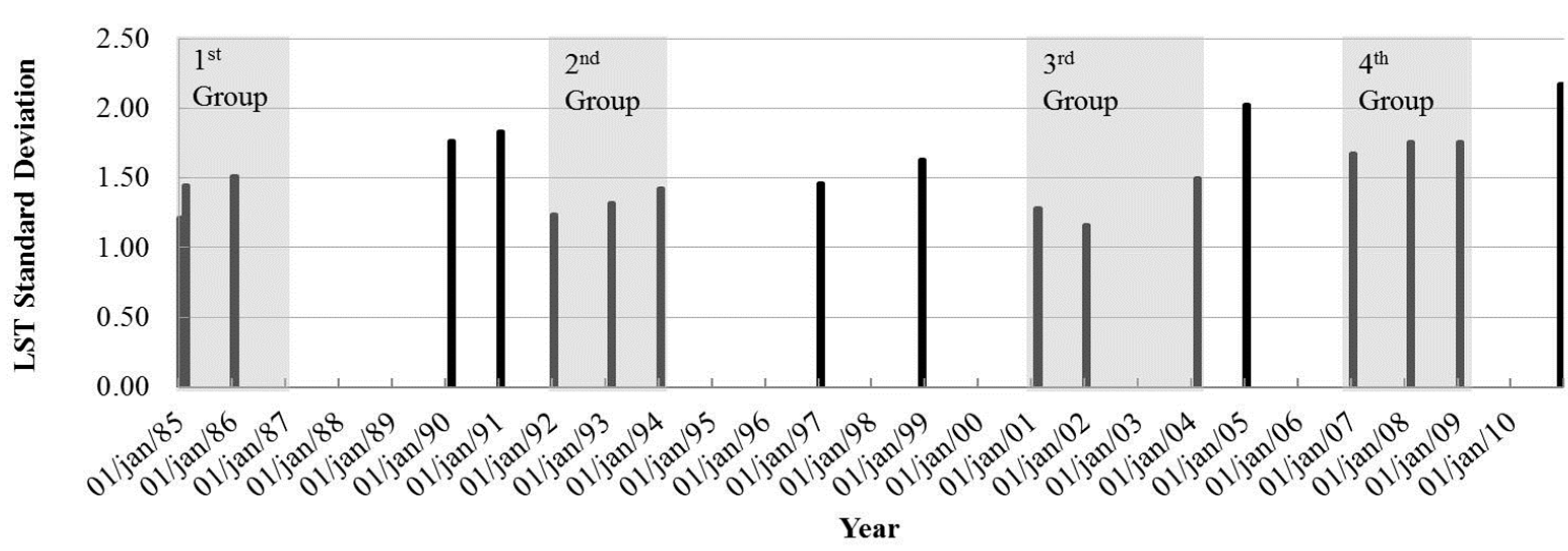
• Individually perform SD analysis of LST distribution for each image available.
• Set groups of images by their temporal proximity.
• Set groups of selected images with similar SD.
• Calculate the average LST for each selected group. Even considering that the average calculation will significantly change the LST values, this processing step is important because the aim is to preserve the spatial distribution characteristic, not the values.
• Calculate the LST average in the entire study area, which are 47 neighborhoods in this case, on a pixel basis. This step is important to the evaluation of the LST deviation from the first image. It is important to note that, although no conclusion can be observed about the variation of the LST values through time, caused by temperature and weather seasonality, the spatial characteristics of LST distribution, are preserved.
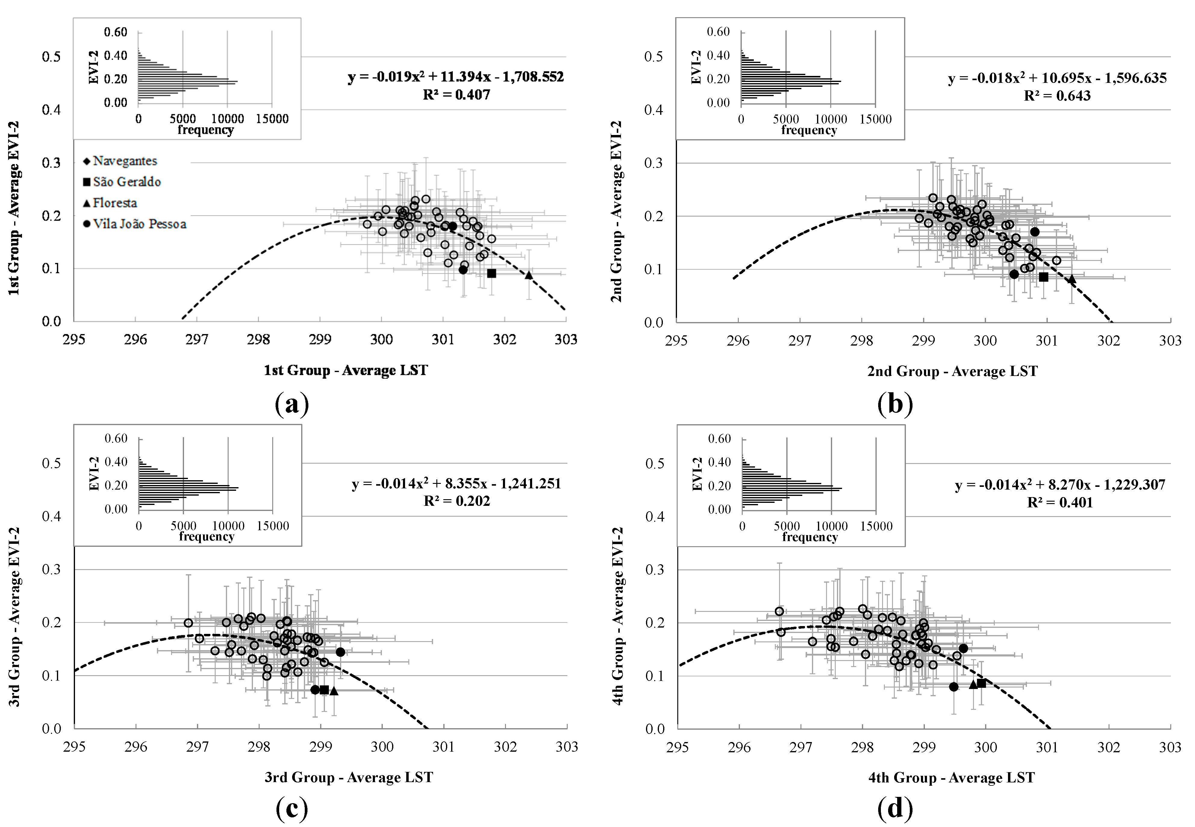
• Compare the imagery data between neighborhoods. A scatterplot comparing LST with EVI-2 on a neighborhood basis can show the LST trend of neighborhoods through time in the multi-temporal imagery data.

The analysis of vegetation coverage conditions using the LST distribution indicated that in the first period, a wide range of LST was associated with high fractions of impervious surfaces or degraded vegetation conditions. The analysis of EVI-2 distribution indicated that vegetation coverage density did not increase in the neighborhoods; however, there has been an overall spread of vegetation coverage areas.

There are several conditions of LULC related to seasonal characteristics and urban environment development, which can cause variability of SD. Figure 2 shows bar-chart diagrams for the 18 dates monitored between 1985 and 2010. A highly variable trend of LST distribution through time was observed, caused by its characteristics of urbanization and development. The general variation of SD values was between 1.16 and 2.17. This figure also shows the groups of images selected to perform the analysis. For group formation, only 12 images were selected (three for each group). Regarding the grouping step of LST, which combines the three available images for each group in a simple average, the obtained LST variation for each group was 294.94 to 305.43 K (average = 300.89 K) in the first group; 294.89 to 304.20 K (average = 299.93 K) in the second group; 292.66 to 303.12 K (average = 298.35 K) in the third group; and 292.01 to 305.32 K (average = 298.84 K) in the fourth group.

Figure 2. Standard deviation distribution of LST through time in the study area from 1985 to 2010 and selected groups obtained with TSDS procedure.

Figure 2. Standard deviation distribution of LST through time in the study area from 1985 to 2010 and selected groups obtained with TSDS procedure.

Combining all imagery data, it is possible to identify the major patterns of LST distribution. The overall average of the LST, from all 18 images selected, was 300.23 K (27.8 °C) with a standard deviation of 1.25 K with the maximum average difference of 2.83 K between the neighborhoods. The intra-period averages were 1.23, 1.20, 1.18 and 1.58 for the first, second, third and fourth periods, respectively. It is also important to note that the intra-period of SD was in agreement with the general behavior of the multi-temporal data. This result indicates that the LST distribution adheres to the evaluated physical concept of vegetation coverage in the two different studied periods. Figure 3 shows the LST averages obtained from all selected images in the study area.

Figure 3. Average of LST between 1985 and 2010 and estimated UHI in Porto Alegre municipality with the streets in the neighborhoods highlighted: (A) Floresta and (B) Vila João Pessoa.

Figure 3. Average of LST between 1985 and 2010 and estimated UHI in Porto Alegre municipality with the streets in the neighborhoods highlighted: (A) Floresta and (B) Vila João Pessoa.

3. Results and Discussion

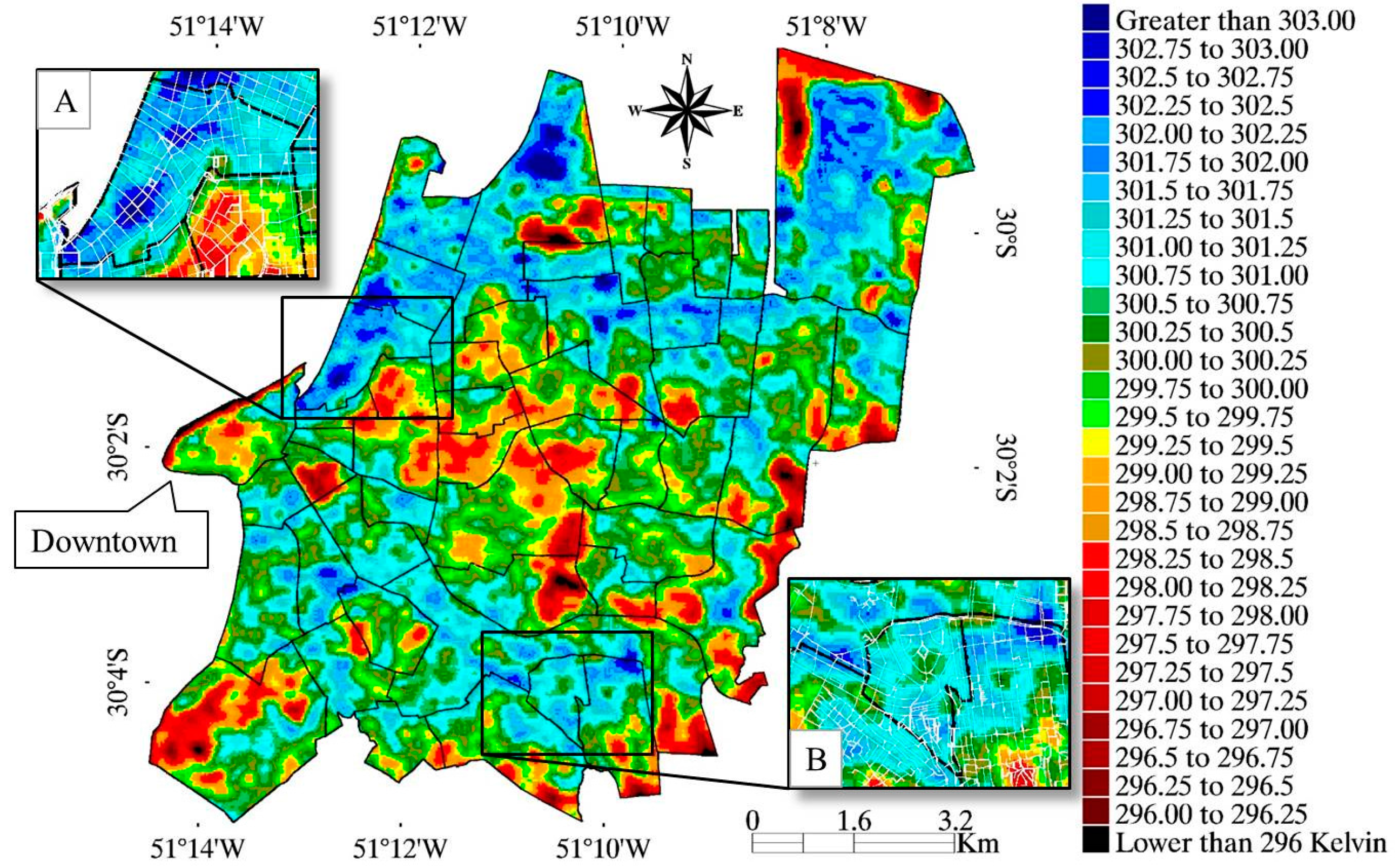
Validation Comparison for UHI Identification

After the formation of groups by the TSDS approach, the imagery data between neighborhoods can be compared. Figure 4 shows scatterplots of the LST trend of neighborhoods through time in the multi-temporal imagery data.

The validation step, which compares the obtained results of TSDS estimates with those obtained from EVI-2, for the evaluation of vegetation cover, indicated that the two estimates were in good agreement. The LST and EVI-2 distributions inside the urban environment, as shown in Figure 4, revealed a wider range of LST in the fourth period than in the previous ones.

The most pronounced variation occurred in the neighborhoods that received the train line in 1985. The train line goes from downtown in the west towards the north. LST colors in dark blue and dark red represent the highest and lowest temperatures, respectively. Results also show that the SD of LST distribution is related to the amount of green vegetated areas and urban environment conditions [17]. This is in agreement with the expected inverse mathematical relation based on the physical assumption that LST and EVI-2 data, at a given pixel, vary inversely over time. To better understand the LST distribution of an urban environment, all data were compared using non-linear regression analysis. We expect to find better correlations by using a negative second-order polynomial relation as described by the mathematical equation y = −α × x² + β × x + γ.

Figure 4. Scattergram of the estimated LST distribution in the urban area of Porto Alegre municipality, considering the 47 neighborhoods within the four groups (a–d), respectively.

Figure 4. Scattergram of the estimated LST distribution in the urban area of Porto Alegre municipality, considering the 47 neighborhoods within the four groups (a–d), respectively.

By considering the bioclimatic conditions of vegetation coverage in the urban environment, the challenge is to understand what represents vegetation development. Background contamination can actually promote imbalance in the relation between bands 3 and 4 (EVI-2 calculation), potentially leading to decreases in the resulting EVI-2 values under the influence of wetland areas. Regarding the seasonal effects and fluctuation of vegetation cover conditions, it is well known that in drought-free years, well-developed vegetation reflects only a small portion of incident solar radiation in the visible band of the spectrum because of chlorophyll absorption properties and other plant pigments that absorb sunlight [54]. In the NIR, plants reflect much more because of a scattering effect caused by the internal structure and water content of leaves [55]. The performance of the TSDS was validated by LST distribution analysis in relation to the vegetation index EVI-2 data. This analysis relates the LST to the vegetated land coverage capacity to perform evapotranspiration.

On the neighborhood scale, results show a non-linear inverse correlation (R² = 0.55) between vegetation index and LST.

An important challenge is to understand how can some increase of standard deviation of LST values occur without any change, or a small change, of general conditions in the EVI-2. One explanation is to increase the built and impervious areas with the increase of neighborhood development. Hence, it can be understood that the temperature of the areas increases while maintaining the same overall conditions of the EVI-2. These areas result in spreading a forward variation of LST, resulting in a smoothing on the curve as can be seen in Figure 4b–d.

Although daily weather variations of temperatures can actually mask the range of LST distribution, a slight decrease in the EVI-2 values, below 0.1 units, was associated with the neighborhoods in the third and fourth groups. A decreasing trend of the total vegetated areas was also observed by analyzing the EVI-2 distribution. In this way, it is worthwhile to note that in recent years, as the overall vegetation cover conditions remained almost the same, the built and impervious areas were intensified because of an increase in the surrounding commercial and economical activities. This increase is particularly true towards the northern neighborhoods (Floresta, Navegantes e São Geraldo), which have had the train line since 1985.

To explain the changes in the temperature pattern occurring in the three districts of Porto Alegre, we assume an urban metabolism concept. This concept performs an analogy between an organism and a city in which there is a stream of inflows and outflows to the urban system, storage of energy, water, materials, nutrients and waste [56]. According to [57], the metabolic flux of a city is influenced by factors such as land use, spatial configuration, population density, population size, economic status, infrastructure and lifestyle of its residents. The analysis of these indicators and their relation to the metabolic flux of a city are crucial for understanding urban metabolism, and hence, in the case of our study, may help to explain the increase in LST occurring in three northern neighborhoods over the 25-year period.

Conducting a study in the United States, for cities with a population over 100,000 [3], observed that urban forests were highly related to income. Considering Porto Alegre, each neighborhood has different characteristics caused by the patterns of urban development prevailing over the past decades. In the case of Floresta, Navegantes and São Geraldo neighborhoods, two factors stand out. The first one is related to the presence of the train line since 1985, and some large avenues, which have access roads into and out of the city, and are present in the two districts; the second one concern the existence of industrial plants, corporate services and companies located in these regions.

The two factors may be somewhat inter-related to the increase of pollution, population decline and imbalance in land use. As observed by [3], tree presence reflects, to some extent, the market forces determined by the welfare of the citizens. In these neighborhoods, results indicate that the most pronounced increase of average LST was associated with the installation of surface train facilities in April 1985 and occurred in two periods. In the first period, the higher LST averages immediately occurred in the neighborhoods directly associated with the train line. In the second period, an increase in the average LST was observed in some adjacent neighborhoods. This spreading area of average LST coverage was primarily identified to occur towards the north of the city’s downtown border (west sites) in developing new neighborhoods. However, an increase in the average LST was not detected in the new vegetated areas of the same neighborhoods.

A different approach must be considered to the case of Vila João Pessoa, which appears to exhibit another particular behavior of urban environment development. Vila João Pessoa is the first suburban neighborhood, constructed around 1940, developed with the same sub-standard conditions and without adequate planning [58], maintaining the same poor conditions of infrastructure, residential and high population density and vegetated areas and low standard trees for years. Most of its population live in a society with no fixed job, and survive on the collection of waste (industrial waste, plastic bottles). In 2010, the average income of residents of Vila João Pessoa was 3.23 salary units, with the average for the entire Porto Alegre city being 5.3 salary units. Higher and lower salary units income were observed in neighborhoods which are far away from downtown and were not included in the study area, namely Pedra Redonda and Serraria, with 18.24 and 5.24 salary units, respectively.

Although it is possible that reduced public health policies contribute to the precarious situation, which leads to the strengthening of low educational status regarding the need for environmental preservation [58]. The identification of such patterns may help develop strategies and overcome obstacles in the urban environment, promoting sustainability and quality of life [59].

4. Conclusions

Our results show that TSDS analysis can help multi-temporal studies for the evaluation of UHI through time. Although the multi-temporal study of UHI is a difficult task, mainly caused by temperature and weather seasonality, the TSDS approach can be used for imagery selection and pre-processing analysis.

The TSDS approach preserves the features and spatial distributions of LULC conditions in the urban environment for the identification of different levels of development on a neighborhood scale. Additionally, the association between the LST and EVI-2 on the neighborhood level demonstrated to be straightforward for UHI studies.

In summary, based on the concept of urban metabolism, some factors, such as land use and spatial configuration of urban areas, can be analyzed together over the years for a better understanding of UHI at the neighborhood scale.

For further study, more accurate results for a pixel basis analysis can be obtained by artificial neural network training parameters. In this context, the launch of the LDCM on 11 February 2013 and TSDS can further assist the management of local and regional urban areas by providing reliable spatial information.

References

1. Brown, L. World on the Edge; W. W. Norton & Company: New York, NY, USA, 2011; p. 325. [Google Scholar]
2. Shen, L.; Kyllo, J.M.; Guo, X. An Integrated Model Based on a Hierarchical Indices System for Monitoring and Evaluating Urban Sustainability. Sustainability 2013, 5, 524–559. [Google Scholar]
3. Zhu, P.; Zhang, Y. Demand for urban forests in United States cities. Land. Urban Plan. 2008, 84, 293–300. [Google Scholar]
4. Voogt, J.A.; Oke, T.R. Thermal remote sensing of urban climates. Remote Sens. Environ. 2003, 86, 370–384. [Google Scholar]
5. Landsberg, H.E. The Urban Climate; Academic Press: New York, NY, USA, 1981. [Google Scholar]
6. Weng, Q.; Lu, D.; Schubring, J. Estimation of Land Surface Temperature—Vegetation Abundance Relationship for Urban Heat Island Studies. Remote Sens. Environ. 2004, 89, 467–483. [Google Scholar]
7. Gusso, A. Integração de Imagens NOAA/AVHRR: Rede de Cooperação para Monitoramento Nacional da Safra de Soja. Rev. Ceres. 2013, 60, 194–204. (In Portuguese) [Google Scholar]
8. Chudnovsky, A.; Ben-Dor, E.; Saaroni, H. Diurnal thermal behavior of selected urban objects using remote sensing measurements. Energy Build. 2004, 36, 1063–1074. [Google Scholar]
9. United States Environmental Protection Agency (EPA). Reducing Urban Heat Islands: Compendium of Strategies-Trees and Vegetation. 2008. Available online: http://www.epa.gov/heatisland/resources/compendium.htm (accessed on 2 July 2012). [Google Scholar]
10. Bruntland, G. Our Common Future: The World Commission on Environment and Development. Oxford University Press: New York, NY, USA, 1987. [Google Scholar]
11. Li, J.; Song, C.; Cao, L.; Zhu, F.; Meng, X.; Wu, J. Impacts of Landscape Structure on Surface Urban Heat Islands: A Case Study of Shanghai, China. Remote Sens. Environ. 2011, 115, 3249–3263. [Google Scholar]
12. Quattrochi, D.A.; Ridd, M.K. Measurement and analysis of thermal energy responses from discrete urban surfaces using remote sensing data. Int. J. Remote Sens. 1994, 15, 1991–2022. [Google Scholar]
13. Kogan, F.N. World Droughts in the New Millennium from AVHRR-based Vegetation Health Indices. Eos Trans. 2002, 83, 557–564. [Google Scholar]
14. Owen, T.W.; Carlson, T.N.; Gillies, R.R. Remotely sensed surface parameters governing urban climate change. Int. J. Remote Sens. 1998, 19, 1663–1681. [Google Scholar]
15. Sobrino, J.A.; Oltra-Carrió, R.; Sòria, G.; Bianchi, R.; Paganini, M. Impact of spatial resolution and satellite overpass time on evaluation of the surface urban heat island effects. Remote Sens. Environ. 2012, 117, 50–56. [Google Scholar]
16. Wong, M.S.; Nichol, J.E. Spatial variability of frontal area index and its relationship with urban heat island intensity. Int. J. Remote Sens. 2013, 34, 885–896. [Google Scholar]
17. Gusso, A.; Veronez, M.R.; Robinson, F.; Roani, V.; Da Silva, R.C. Evaluating the thermal spatial distribution signature for environmental management and vegetation health monitoring. Int. J. Adv. Remote Sens. GIS 2014, 3, 433–445. [Google Scholar]
18. Rao, P.K. Remote sensing of urban “heat islands” from an environmental satellite. Bull. Am. Meteorol. Soc. 1972, 53, 647–648. [Google Scholar]
19. Callejas, I.J.A.; Oliveira, A.S.; Santos, F.M.M.; Durante, L.C.; Nogueira, M.C.J.A.; Zeilhofer, P. Relationship between land use/cover and surface temperatures in the urban agglomeration of Cuiabá-Várzea Grande, Central Brazil. J. Appl. Remote Sens. 2011, 5, 1–15. [Google Scholar]
20. Irons, J.R.; Dwyer, J.L.; Barsi, J.A. The Next Landsat Satellite: The Landsat Data Continuity Mission. Remote Sens. Environ. 2012, 122, 11–21. [Google Scholar]
21. Ogashawara, I.; Bastos, V.S.B. A Quantitative Approach for Analyzing the Relationship between Urban Heat Islands and Land Cover. Remote Sens. 2012, 4, 3596–3618. [Google Scholar]
22. Köppen, W. Climatologia: Con un Estúdio de los Climas de la Tierra; Fondo de Cultura Econômica: Tlalpan, Mexico, 1948; p. 466. (In Spanish) [Google Scholar]
23. Instituto Brasileiro de Geografia e Estatística (IBGE). Available online: http://www.ibge.gov.br/english/ (accessed on 2 July 2012).
24. Instituto Nacional de Meteorologia (INMET). Available online: http://www.inmet.gov.br/portal/index.php?r=bdmep/bdmep (accessed on 12 January 2011).
25. Instituto Nacional de Pesquisas Espaciais (INPE). Available online: www.dgi.inpe.br (accessed on 12 January 2011).
26. Landsat Science (NASA). Available online: http://landsat.gsfc.nasa.gov/ (accessed on 12 June 2011).
27. Chander, G.; Markham, B.L.; Helder, D.L. Summary of Current Radiometric Calibration Coefficients for Landsat MSS, TM, ETM+, and EO-1 ALI Sensors. Remote Sens. Environ. 2009, 113, 893–903. [Google Scholar]
28. Rabus, B.M.; Eineder, A.R.R. The Shuttle Radar Topography Mission—A New Class of Digital Elevation Models Acquired by Space Borne Radar. Photogramm. Eng. Remote Sens. 2003, 57, 241–262. [Google Scholar]
29. Markham, B.L.; Barker, J.L. Thematic Mapper Band pass Solar Exoatmospherical Irradiances. Int. J. Remote Sens. 1987, 8, 517–523. [Google Scholar]
30. Chavez, P.S., Jr. Image-Based Atmospheric Correction—Revisited and Improved. Photogramm. Eng. Remote Sens. 1996, 62, 1025–1036. [Google Scholar]
31. Schroeder, T.A.; Cohen, W.B.; Song, C.; Canty, M.J.; Yang, Z. Radiometric Correction of Multi-Temporal Landsat Data for Characterization of Early Successional Forest Patterns in Western Oregon. Remote Sens. Environ. 2006, 103, 16–26. [Google Scholar]
32. Sobrino, J.A.; Jiménez-Munõz, J.C.; Paolini, L. Land Surface Temperature Retrieval from LANDSAT TM 5. Remote Sens. Environ. 2004, 90, 434–440. [Google Scholar]
33. Jiang, Z.; Huete, A.R.; Didan, K.; Miura, T. Development of a Two-Band Enhanced Vegetation Index without a Blue Band. Remote Sens. Environ. 2008, 112, 3833–3845. [Google Scholar]
34. Liu, J.; Pattey, E.; Jégo, G. Assessment of Vegetation Indices for Regional Crop Green LAI Estimation from Landsat Images over Multiple Growing Seasons. Remote Sens. Environ. 2012, 123, 347–358. [Google Scholar]
35. Weng, Qi. Thermal Infrared Remote Sensing for Urban Climate and Environmental Studies: Methods, Applications, and Trends. ISPRS J. Photogramm. Remote Sens. 2009, 64, 335–344. [Google Scholar]
36. Qin, Z.; Karnieli, A.; Berliner, P. A Mono-Window Algorithm for Retrieving Land Surface Temperature from Landsat TM Data and its Application to the Israel-Egypt Border Region. Int. J. Remote Sens. 2001, 22, 3719–3746. [Google Scholar]
37. Ma, Y.; Kuang, Y.; Huang, N. Coupling Urbanization Analyses for Studying Urban Thermal Environment and its Interplay with Biophysical Parameters Based on TM/ETM+ Imagery. Int. J. Appl. Earth Observ. Geoinf. 2010, 12, 110–118. [Google Scholar]
38. Wukelic, G.E.; Gibbons, D.E.; Martucci, L.M.; Foote, H.P. Radiometric Calibration of Landsat Thematic Mapper Thermal Band. Remote Sens. Environ. 1989, 28, 339–347. [Google Scholar]
39. Cooper, D.I.; Asrar, G. Evaluating Atmospheric Correction Models for Retrieving Surface Temperatures from the AVHRR Over A Tall Grass Prairie. Remote Sens. Environ. 1989, 27, 93–102. [Google Scholar]
40. Waters, R; Allen, R.; Batiassen, W.; Tasumi, M.; Trezza, R. SEBAL (Surface Energy Balance Algorithms for Land)—Idaho Implementation—Advanced Training and User’s Manual. 2002. Available online: ftp://ftp.funceme.br/Cospar_Funceme_2010/CLASS_DAY_04.11.2010/LAB/quixere/quixere/Final%20Sebal%20Manual.pdf (accessed on 17 February 2015).
41. Gusso, A.; Fontana, D.C.; Gonçalves, G.A. Mapeamento da Temperatura da superfície terrestre com uso do sensor NOAA/AVHRR. Pesq. Agropecuária Bras. 2007, 42, 231–237. [Google Scholar]
42. Andersen, H.S. Land Surface Temperature Estimation Based on NOAA-AVHRR Data during the HAPEX-Sahel Experiment. J. Hydrol. 1997, 189, 788–814. [Google Scholar]
43. Sandholt, L.; Rasmussen, K.; Andersen, J. A Simple Interpretation of the Surface Temperature/Vegetation Index Space for Assessment of Surface Moisture Status. Remote Sens. Environ. 2002, 79, 213–224. [Google Scholar]
44. Yuan, F.; Bauer, M.E. Comparison of impervious surface area and normalized difference vegetation index as indicators of surface urban heat island effects in Landsat imagery. Remote Sens. Environ. 2007, 106, 375–386. [Google Scholar]
45. Valor, E.; Casselles, V. Mapping Land Surface Emissivity from NDVI: Application to European, African, and South American Areas. Remote Sens. Environ. 1996, 57, 167–184. [Google Scholar]
46. Campbell, J.B.; Wynne, R.H. Introduction to Remote Sensing; The Guilford Press: New York, NY, USA, 2011; p. 3. [Google Scholar]
47. Bottyán, Z.; Unger, J. A Multiple Linear Statistical Model for Estimating the Mean Maximum Urban Heat Island. Theor. Appl. Climatolog. 2003, 75, 233–243. [Google Scholar]
48. Nemani, R.; Pierce, L.; Running, S. Developing Satellite-Derived Estimates of Surface Moisture Status. J. Appl. Meteorolog. 1993, 32, 548–557. [Google Scholar]
49. Lambin, E.F.; Ehrlich, D. Combining Vegetation Indices and Surface Temperature for Land-Cover Mapping at Broad Spatial Scales. Int. J. Remote Sens. 1995, 16, 573–579. [Google Scholar]
50. Sims, D.A.; Rahman, A.F.; Cordova, V.D.; El-Masri, B.Z.; Baldocchi, D.D.; Bolstad, P.V.; Flanagan, L.B.; Goldstein, A.H.; Hollinger, D.Y.; Misson, L.; et al. A New Model of Gross Primary Productivity for North American Ecosystems Based Solely on the Enhanced Vegetation Index and Land Surface Temperature from MODIS. Remote Sens. Environ. 2008, 112, 1633–1646. [Google Scholar]
51. Schelenker, W.; Roberts, M. Nonlinear Temperature Effects Indicate Severe Damages to U.S. Crop Yields Under Climate Change. Proc. Natl. Acad. Sci. USA 2009, 106, 15594–15598. [Google Scholar]
52. Carmo-Silva, A.E.; Gore, M.A.; Andrade-Sanchez, P.; French, A.N.; Hunsaker, D.J.; Salvucci, M.E. Decreased CO2 Availability and Inactivation of Rubisco Limit Photosynthesis in Cotton Plants under Heat and Drought Stress in the Field. Environ. Exp. Bot. 2012, 83, 1–11. [Google Scholar]
53. Weng, Q.; Lu, D. A sub-pixel analysis of urbanization effect on land surface temperature and its interplay with impervious surface and vegetation coverage in Indianapolis, United States. Int. J. Appl. Earth Observ. Geoinf. 2008, 10, 68–83. [Google Scholar]
54. Gusso, A.; Ducati, J.R. Algorithm for Soybean Classification Using Medium Resolution Satellite Images. Remote Sens. 2012, 4, 3127–3142. [Google Scholar]
55. Jensen, J.R. Remote Sensing of the Environment: An Earth Resource Perspective; Prentice Hall: Upper Saddle River, NJ, USA, 2007; p. 592. [Google Scholar]
56. Kennedy, C.; Pincetl, S.; Bunje, P. The study of urban metabolism and its applications to urban planning and design. Environ. Pollt. 2011, 159, 1965–1973. [Google Scholar]
57. Minx, J.; Creutzig, F.; Medinger, V. Developing a pragmatic approach to assess urban metabolism in Europe—A report to the European environment agency. Available online: http://ideas.climatecon.tu-berlin.de/documents/wpaper/CLIMATECON-2011–01.pdf (accessed on 17 September 2014).
58. Brazil—Prefeitura Municipal de Porto Alegre (PMPA). Centro de Pesquisa Histórica. Coordenação de Memória Cultural da Secretaria Municipal de Cultura. Available online: http://lproweb.procempa.com.br/pmpa/prefpoa/observatorio/usu_doc/historia_dos_bairros_de_porto_alegre.pdf (accessed on 29 September 2014). (In Portuguese)
59. Manning, W.J. Urban environment: Defining its nature and problems and developing strategies to overcome obstacles to sustainability and quality of life. Environ. Pollut. 2011, 159, 1963–1964. [Google Scholar]