Optimum Fisheries Management under Climate Variability: Evidence from Artisanal Marine Fishing in Ghana

Abstract

In most developing coastal countries, the artisanal fisheries sector is managed as a common pool resource. As a result, such fisheries are overcapitalized and overfished. In Ghana, in addition to anthropogenic factors, there is evidence of rising coastal temperature and its variance, which could impact the environmental carrying capacity of the fish stock. This study investigates the effect of climate variation on biophysical parameters and yields. Our results indicate that the rising temperature is decreasing the carrying capacity. As a result, an optimum tax on harvest must reflect climate variability, as well as the congestion externality.

1. Introduction

In spite of the plethora of policies aimed at sustaining capture fish stocks around the world, evidence abound that most stocks are heavily overexploited [1,2]. In developing coastal countries where fishery sectors directly employ significant numbers of people and regulations are generally inadequate, food security and sustainable livelihoods are directly threatened [3,4]. In Sub-Saharan Africa, for example, the fisheries sector directly employs close to three million people and additional 7.5 million people are engaged in fish processing and trading. In addition, it is estimated that in Africa the current annual revenue from capture fishery (US$2 billion) generates a multiplier effect of 2.5 times (US$5 billion) through trickle-up linkages [5]. The high number of fishers in coastal developing countries is due to a growing poverty trap.

In Ghana, artisanal and semi-industrial fishing are the most important direct and indirect employment generating activities within the entire coastal zone. The artisanal sector supported about 1.5 million people (about 9% of the total population) and landed about 70%–80% of total marine catches in 1996 [6]. 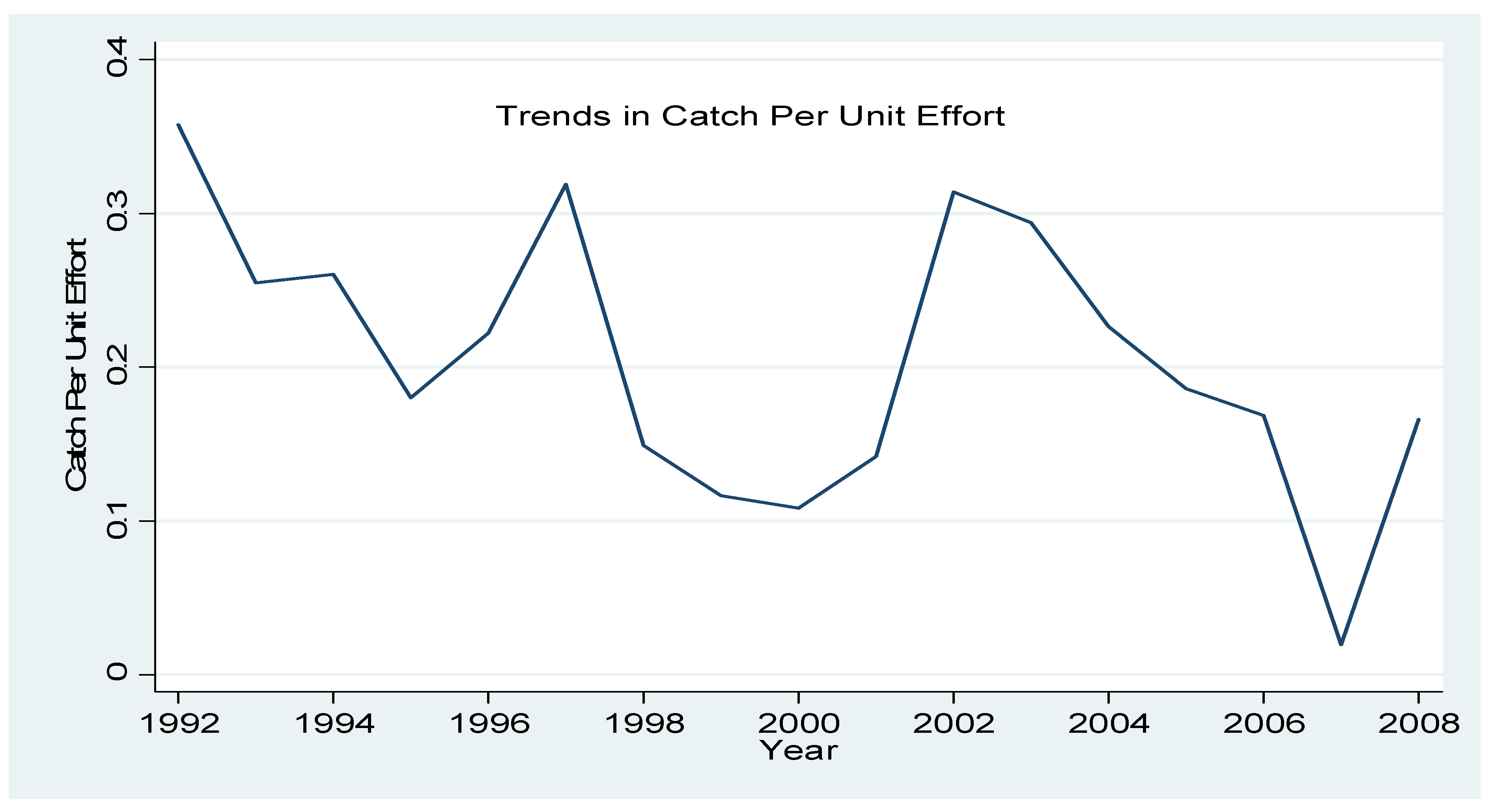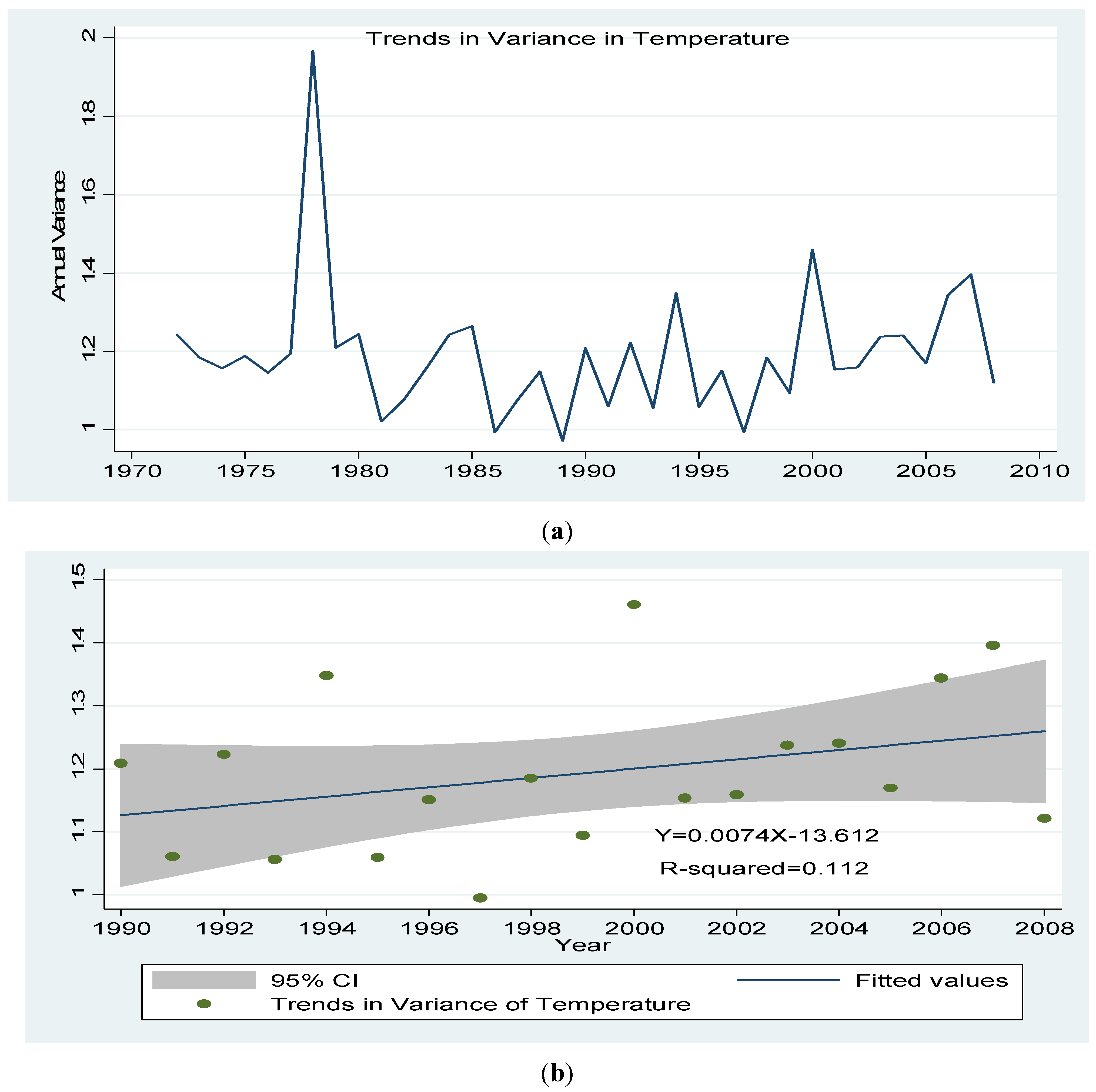The artisanal and semi-industrial fisheries are managed as unregulated common pool resources (CPR), hence are overcapitalized resulting in biological overfishing (i.e., declining catch per unit effort (CPUE)). The existing regulations include a ban on the use of light aggregation equipment, which involves shinning light in the ocean, when the moon is out, to attract fish and increase harvest; a ban on the use of mesh sizes smaller than an inch in stretch diagonal; and a ban on the use of explosives in fishing. These regulations aim at limiting fishing efforts which is on the rise. For example, after a sharp increase in artisanal catch per unit effort between 1989 and 1992, it declined from 1992 through 2008 although fishing techniques improved and the number of crew per boat also increased. Within the same period, available data shows the annual coastal temperature and its variance has been on the rise. Since pelagic stocks targeted by artisanal fishers feed on planktons that depend on seasonal upwelling, it is likely that the rising coastal temperature is impacting the catch per unit effort. Although favorable upwelling can increase with global warming, the rising temperature could impact other environmental conditions for spawning, recruitment, or larval development, among others [7,8].

To reduce fish catches to sustainable levels, an optimum market-based policy instrument such as a tax on cost per unit effort or harvest is necessary. However, the efficacy of such a policy instrument hinges on the knowledge of the biophysical dynamics of the stocks. Two recent studies have shown that a fish stock could be potentially depleted if the biodynamic is misperceived, even if catch policies exist [9,10]. Using time series data on artisanal marine fishing in Ghana (1972–2007), this study (1) extends the existing surplus production function to account for the impact of changes in atmospheric temperature and its variance on the environmental carrying capacity of artisanal fish stock; (2) estimates the biophysical parameters employing the generalized maximum entropy (GME) estimators, which addresses the classical linear regression problems of endogeneity, multi-collinearity, and limited observations; and (3) estimates the optimum tax necessary to internalize congestion externality and the climate impact on fish yield; and forecasts the local atmospheric temperature as well as discusses its implication for the optimum tax. The results showed that the rising temperature yields negative biological response by decreasing the carrying capacity. In addition, a univariate analysis of the annual coastal temperature indicated that it will continue to rise at least in the near future. As a result, the tax rate must be set high enough to account for the increasing temperature in order to protect the artisanal fish stock.

The remainder of the paper is organized as follows. Section 2 presents the optimal control model for the optimal tax, and this is followed by incorporating the atmospheric forcing in the surplus production function in Section 3. Section 4 contains the empirical model and discussion on the estimation method. Section 5 provides the preliminary results and the final section, Section 6, concludes the paper.

2. The Model for Optimum Tax

To briefly outline the model for obtaining the optimum tax, following Akpalu [11], suppose a fishery is managed as a CPR. Let the biomass ($x$) of the fish stock grow according to a logistic function $g\left(x,k\right)$, where $k$ is a constant environmental carrying capacity $g_x(\cdot )>0$ and $g_{xx}(\cdot )\le 0$. For analytical convenience let the logistic growth function be $g\left(x,k\right)=rx\left(1-\frac{x}{k}\right)$, where $r$ is intrinsic growth rate. Furthermore, let $c(x)$ and $p$ be cost per unit harvest and price per kg of fish, respectively. In addition, assume future benefits and costs are discounted at a positive rate, $\mathrm{\delta }$. The value function of the entire fishery is given by Equation (1) and the stock dynamic Equation (2).

$$V(x,H)=\underset{H}{max}{\displaystyle \underset{0}{\overset{\mathrm{\infty }}{\int }}\left(pH-c(x)H\right)}{e}^{-\mathrm{\delta }t}dt$$

(1)

$$\dot{x}=rx\left(1-\frac{x}{k}\right)-H , \mathrm{with} H={\displaystyle \sum _{i=1}^n{h}_i}$$

(2)

where $\dot{x}=\frac{dx}{dt}$, $H$ is aggregate harvest, and $h_i$ is the harvest of one economic agent ($i$). The corresponding current value Hamiltonian of the programme is

$$\mathrm{\Gamma }\left(x,H,\mathrm{\mu }\right)=\left(pH-c(x)H\right)+\mathrm{\mu }\left(rx\left(1-\frac{x}{k}\right)-H\right)$$

(3)

where $\mathrm{\mu }$ is the scarcity value of the fish stock.

From the maximum principle, assuming an interior solution exists, the first order condition with respect to harvest ($H$) is

$$\frac{\partial \mathrm{\Gamma }(.)}{\partial H}=p-c(x)-\mathrm{\mu }=0$$

(4)

Equation (4) simply stipulates that in an inter-temporal equilibrium harvest must be at a level that equates net marginal benefit (i.e., $p-c(x)$) to the scarcity value of the stock (i.e., $\mathrm{\mu }$). If $p-c(x)>\mathrm{\mu }$, harvest has to be at its maximum. On the other hand it must be set to zero if $p-c(x)<\mathrm{\mu }$. The corresponding costate equation is

$$\dot{\mathrm{\mu }}-\mathrm{\delta }\mathrm{\mu }=-\frac{\partial H(.)}{\partial x}=c_{x}H-\mathrm{\mu }r\left(1-\frac{2x}{k}\right)$$

(5)

Equation (5) implies that, in dynamic equilibrium, the interest earnable on the net marginal benefit from harvesting one kilogramme of fish today (i.e., $\mathrm{\delta }\mathrm{\mu }$) must equate the sum of the capital gain from conserving that kilogramme of fish (i.e., $\dot{\mathrm{\mu }}$) and some stock effect (i.e., $-c_{x}H+\mathrm{\mu }r\left(1-2x{k}^{-1}\right)$). In steady state $\dot{x}=\dot{\mathrm{\mu }}=0$ so that Equations (4) and (5) become

$$p-c(x)=-c_x\left(rx\left(1-\frac{x}{k}\right)\right){\left(\mathrm{\delta }-r\left(1-\frac{2x}{k}\right)\right)}^{-1}$$

(6)

Now suppose the stock is harvested as a CPR by $n$ users. Following Maler et al. [12] and Akpalu [11], the optimization programme for each community is

$$V(x,h_i)=\underset{h_i}{max}{\displaystyle \underset{0}{\overset{\mathrm{\infty }}{\int }}\left(p-c(x)\right)h_i}{e}^{-\mathrm{\delta }t}dt,i=1,2,\mathrm{...},n$$

(7)

$$\dot{x}=rx\left(1-\frac{x}{k}\right)-{\displaystyle \sum _i^n{h}_i},H={\displaystyle \sum _i^n{h}_i}$$

(8)

The corresponding first order condition from the maximum principle is

$$\frac{\partial Z(.)}{\partial h_i}=p-c(x)-{\mathrm{\mu }}_i=0,i=1,2,\mathrm{...},n$$

(9)

The shadow value assigned to the resource by each symmetric community is ${\mathrm{\mu }}_i=\frac{\mathrm{\mu }}{n}$. The symmetric open-loop Nash equilibrium solution is

$$p-c(x)=\frac{\mathrm{\mu }}{n}=-c_x\left(rx\left(1-\frac{x}{k}\right)\right){\langle n\left(\mathrm{\delta }-r\left(1-\frac{2x}{k}\right)\right)\rangle }^{-1}$$

(10)

Equation (10) could be solved for the equilibrium stock level (i.e., $x^{**}=x(k,n)$). Suppose the resource is harvested as a CPR and let a tax be imposed on cost of harvest (i.e., $c(x)\left(1+\mathrm{\tau }\right)$) to generate the first best solution. The equilibrium stock equation with the tax is

$$p-c(x)\left(1+\mathrm{\tau }\right)=-c_x\left(1+\mathrm{\tau }\right)\left(rx\left(1-\frac{x}{k}\right)\right){\langle n\left(\mathrm{\delta }-r\left(1-\frac{2x}{k}\right)\right)\rangle }^{-1}$$

(11)

or

$$n\left(p-c(x)\left(1+\mathrm{\tau }\right)\right){\left(1+\mathrm{\tau }\right)}^{-1}=-c_x\left(rx\left(1-\frac{x}{k}\right)\right){\left(\mathrm{\delta }-r\left(1-\frac{2x}{k}\right)\right)}^{-1}$$

From Equations (6) and (11): $\frac{n\left(p-c(x^{*})\left(1+\mathrm{\tau }\right)\right)}{\left(1+\mathrm{\tau }\right)}=p-c(x^{*})$, which implies

$$tax(\mathrm{\tau })=\frac{p-c\left(x^{*}\right)}{\raisebox{1ex}{$p$}\!\left/ \!\raisebox{-1ex}{$\left(n-1\right)$}\right.+c\left(x^{*}\right)}$$

(12)

If $n>1$, aggregate catch will exceed the socially desirable level and a policy intervention will be required to regulate catch. Using $c(x^{*})=\frac{c}{q{x}^{*}}$ (where $c$ and $q$ are cost per unit effort and catchability coefficient, respectively), the steady state stock $x^{*}$ is

$$x^{*}=\frac{k}{4}\left[\left(\frac{c}{pqk}+1-\frac{\mathrm{\delta }}{r}\right)+\sqrt{\left({\left(\frac{c}{pqk}+1-\frac{\mathrm{\delta }}{r}\right)}^2+\frac{8c\mathrm{\delta }}{pqkr}\right)}\right]$$

(13)

The specific tax expression is based on these specific functional forms. The tax depends on the values of the socio-economic parameters (i.e., $p$, $c$ and $\mathrm{\delta }$), which are readily available, and biological parameters (i.e., $r$, $q$ and $k$) which are not.

Climate Variability and Optimal Tax Rate

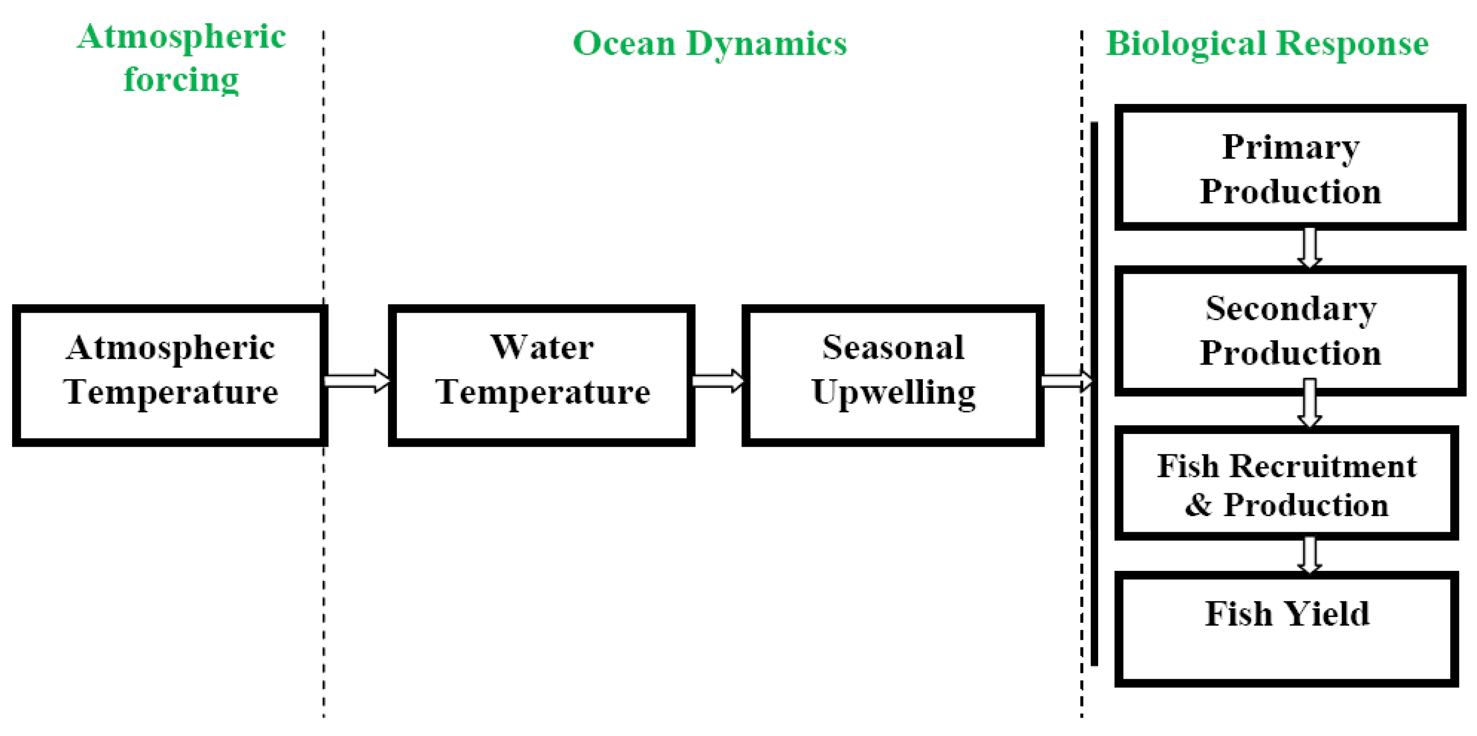
If climate variability impacts the carrying capacity, then the tax rate must reflect potential variability in the climate. As indicated in the introduction, there is overwhelming evidence that climate variability may impact carrying capacity of the stock. Atmospheric forcing may result in a change in atmospheric temperature (see Figure 1). The change in temperature impacts water temperature and subsequently influences seasonal upwelling (or downwelling). This influences primary production, species distribution, fish yield, and increased variability of catches (4).

Figure 1. The flow chart of the impact of atmospheric temperature on fish yield. Source: own compilation.

Figure 1. The flow chart of the impact of atmospheric temperature on fish yield. Source: own compilation.

To account for the impact of atmospheric temperature on fish production, we surmise that the carrying capacity is defined as

$$k=\frac{k_0}{1+\mathrm{\epsilon }\mathrm{\Delta }{T}_t+\mathrm{\eta }{\mathrm{\sigma }}_t}$$

(14)

where $T$ and $\mathrm{\sigma }$ are the state of the climate variable and its variances, respectively; $\mathrm{\Delta }$ is notation for first difference (We used the change in temperature because the levels of the series are within a limited range, given the period considered for the empirical analysis. As expected, the levels were not significant in the empirical analysis (presented in the later section of the paper) but the first differences were.); and $k_0$, $\mathrm{\epsilon }$, and $\mathrm{\eta }$ are constants. The corresponding optimum path of the stock is

$$x^{*}\left(t\right)=\frac{k_0}{4\left(1+\mathrm{\epsilon }\mathrm{\Delta }{T}_t+\mathrm{\eta }{\mathrm{\sigma }}_t\right)}\left[\left(\frac{c\left(1+\mathrm{\epsilon }\mathrm{\Delta }{T}_t+\mathrm{\eta }{\mathrm{\sigma }}_t\right)}{pq{k}_0}+1-\frac{\mathrm{\delta }}{r}\right)+\sqrt{\left({\left(\frac{c\left(1+\mathrm{\epsilon }\mathrm{\Delta }{T}_t+\mathrm{\eta }{\mathrm{\sigma }}_t\right)}{pq{k}_0}+1-\frac{\mathrm{\delta }}{r}\right)}^2+\frac{8c\mathrm{\delta }\left(1+\mathrm{\epsilon }\mathrm{\Delta }{T}_t+\mathrm{\eta }{\mathrm{\sigma }}_t\right)}{pq{k}_{0}r}\right)}\right]$$

(15)

3. Obtaining the Biophysical Parameters

To establish the link between climate variability and fish production, a biological model is employed. In order to estimate the biological parameters, a number of authors have employed models by Schaefer and Fox [13]. These models assume equilibrium or steady state conditions in order to obtain an equation that is used to estimate next period’s catch per unit effort without specifying future anticipated effort [13]. However, Schnute [14] has shown that these models may be invalid for non-equilibrium conditions and the assumption that catch per unit effort could be predicted without specifying future anticipated effort contradicts almost all theory on fisheries biology. As a result, the author suggested a modified version, which is Equation (16)

$$\ln \left(\frac{U_{t+1}}{U_t}\right)=r-\frac{r}{q{k}_0}\left(\frac{U_t+U_{t+1}}{2}\right)-q\left(\frac{E_t+E_{t+1}}{2}\right)$$

(16)

where $U_t=\left(\frac{h_t}{E_t}\right)$ signifies catch per unit effort, and $E_t$ is fishing effort. As indicated in the introduction, there is overwhelming evidence that climate variability may impact carrying capacity of fish stock. Using Equation (14) in Equation (16), gives

$$\ln \left(\frac{U_{t+1}}{U_t}\right)=r-\frac{r}{q{k}_0}\left(\frac{U_t+U_{t+1}}{2}\right)+\frac{r\mathrm{\epsilon }}{q{k}_0}\left(\frac{U_t+U_{t+1}}{2}\right)\mathrm{\Delta }{T}_t+\frac{r\mathrm{\eta }}{q{k}_0}\left(\frac{U_t+U_{t+1}}{2}\right){\mathrm{\sigma }}_t-q\left(\frac{E_t+E_{t+1}}{2}\right)$$

(17)

4. The Empirical Model and Estimation Methods

In this section, the extended Schnute model (i.e., Equation (17)) and an estimation method known as a GME estimator is presented. For the purpose of estimation, Equation (17) is specified as

$$\ln \left(\frac{U_{t+1}}{U_t}\right)=a_0+a_1{\overline{U}}_t+a_2{\overline{U}}_t\mathrm{\Delta }{T}_t+a_3{\overline{U}}_t{\mathrm{\sigma }}_t+a_4{\overline{E}}_t+{\mathrm{\mu }}_t$$

(18)

where ${\overline{U}}_t=\left(\frac{U_t+U_{t+1}}{2}\right)$, ${\overline{E}}_t=\left(\frac{E_t+E_{t+1}}{2}\right)$, $a_0=r>0$, $a_1=-\frac{r}{\mathrm{\sigma }k}<0$, $a_4=-q<0$, and ${\mathrm{\mu }}_t$ is an error term. Time series data on catch, fishing effort, and temperature is required to estimate Equation (18).

4.1. Empirical Estimations: Generalized Maximum Entropy

The obvious problem with applying ordinary least squares estimation procedure to Equation (18) is endogeneity since the dependent variable interacts with other variables on the right hand side. It is also very likely that some of the variables are highly correlated. As a result, the coefficients are estimated using GME, which are explained in the subsequent sections. The GME method could generate reliable estimates of the parameters of our model. The GME is a semi-parametric estimator and belongs to a class of estimators used in engineering and physics. To present the GME estimator, let

$$a_k={\displaystyle \sum _s{z}_{ks}{p}_{ks}}$$

(19)

where $p_{ks}\ge 0$ are unknown probabilities and ${\displaystyle \sum _s{p}_{ks}=1}$; $z_{ks}$ constitutes a predetermined discrete support space ($s$) for the parameters; and $a_k$ is as defined in Equation (18). Furthermore, define the error term in Equation (18) as

$$u_i={\displaystyle \sum _g{V}_{ig}}{w}_{ig}$$

(20)

where $w_{ig}\ge 0$ are unknown probabilities and ${\displaystyle \sum _g{w}_{ig}=1}$; $V_{ig}$ constitutes an a priori discrete support space ($g$) for the errors; and $u_i$ is as defined in Equation (18). The GME estimator is specified as

$$\max H(p_{ks},w_{ig})=-{\displaystyle \sum _s{p}_{ks}}\ln (p_{ks})-{\displaystyle \sum _g{w}_{ig}}\ln (w_{ig})$$

(21)

subject to Equation (18), but with the coefficients and the error term substituted by Equations (19) and (20). The limitation of this method is that the values of the parameters are sensitive to arbitrarily chosen support values making policy recommendations sensitive to such values. The estimations are implemented in general algebraic modeling system (GAMS).

4.2. Data Types and Sources

Data on catch and effort were collected from the Directorate of Fisheries of the Ministry of Food and Agriculture (MOFA) in Ghana. The Directorate is mandated to carry out research for the assessment for fisheries resources. As noted in the introduction, the artisanal fishery sector is one of the most important sectors within the economy. However, recent landing statistics for the artisanal fleet indicate landings peaked in 1992, and then declined due to overexploitation [15]. The data on temperature was collected from Ghana Meteorological Agency. The agency has 17 weather stations each reporting monthly average temperatures. The figure for the standard deviation of temperature is computed from the 12-month averages for each year. The summary statistics of the data is presented in Table 1.

Table 1. Descriptive Statistics of catch, fishing trips and coastal temperature in Ghana.

Variable	1972–2008		1990–2008
	Mean	Standard dev.	Mean	Standard dev.
Catch (in kg)	195,354	53,378	229,212	34,192
Effort (Number of trips)	1,319,614	1,549,476	1,653,440	1,988,563
Temperature (in °C)	27.0	0.419	27.3	0.291
Std. Dev. of temperature	1.193	0.170	1.193	0.124

Source: Catch and effort data is collected from Directorate of Fisheries, Ghana; and temperature data is collected from Ghana Meteorological Agency.

Table 1. Descriptive Statistics of catch, fishing trips and coastal temperature in Ghana.

Variable	1972–2008		1990–2008
	Mean	Standard dev.	Mean	Standard dev.
Catch (in kg)	195,354	53,378	229,212	34,192
Effort (Number of trips)	1,319,614	1,549,476	1,653,440	1,988,563
Temperature (in °C)	27.0	0.419	27.3	0.291
Std. Dev. of temperature	1.193	0.170	1.193	0.124

Source: Catch and effort data is collected from Directorate of Fisheries, Ghana; and temperature data is collected from Ghana Meteorological Agency.

From Table 1, both catch and effort levels have increased over the last 18 years. In addition, as depicted in Figure 2, catch per unit effort oscilates over time. The periods of decline in the CPUE were 1992 to 1995, 1997 to 2000, and 2002 through 2007. On the other hand, the CPUE increased from 1994 to 1997, 2000 to 2002, and 2007 through 2008. On the average, however, the variable shows a weak pattern of decline from 1992 through 2008.

Figure 2. Trends in catch per unit effort of artisanal stocks (1992–2008); Source: own illustration.

Figure 2. Trends in catch per unit effort of artisanal stocks (1992–2008); Source: own illustration.

Furthermore, from Table 1, the mean temperature within the entire period (1972–2007) is lower than that of the last 18 years (1990–2007). The time trend of the atmospheric coastal temperature has revealed a rising trend over time (see Figure 3). Moreover, although the annual variance of the coastal temperature (shown in Figure 4a) (The variance is calculated as the sum of the squared deviation of monthly temperature from the yearly average, divided by 11 (i.e., degrees of freedom).) looks like a stationary process, a careful examination of a segment of the data (from 1990 through 2008) reveals an upward trend with a gentle slope (shown in Figure 4b). The period of 1990 through 2008 witnessed a decline in the catch per unit effort.

Figure 3. Trends in coastal temperature (1972–2008); Source: own illustration.

Figure 3. Trends in coastal temperature (1972–2008); Source: own illustration.

Figure 4. (a) Trends in the variance of coastal temperature (1972–2008); (b) Trends in the variance of coastal temperature (1990–2008); Source: own illustration.

Figure 4. (a) Trends in the variance of coastal temperature (1972–2008); (b) Trends in the variance of coastal temperature (1990–2008); Source: own illustration.

5. Results and Discussions

The biological parameters were estimated using the General Algebraic Modeling System (GAMS). Since the catch intensified beginning 1990, the data for the estimation spans a period of 1990–2007. For the purpose of comparison, two versions of the model were estimated: one without the climate variables and a complete version with the climate impact on carrying capacity. The results of the estimation are reported in Table 2.

Table 2. Estimated biological parameters of the Schnute equation.

Parameters		Estimates
Description	Notation	GME
		1	2
Intrinsic growth rate	$r$	1.91369	1.960
Catchability coefficient *	$q$	0.627 × 10−6	0.636 × 10−6
Carrying capacity (in kg)	$k_0$	530,066	449,683
Impact of temperature on $k$	$\mathrm{\epsilon }$		0.166244
Impact of temperature variation on $k$	$\mathrm{\eta }$		0.115561
Pseudo R-squared		0.70	0.73

Source: own computations. * Using surplus production functions, Clarke et al. [13] estimated the catchability coefficient to be within the range of 0.376 × 10⁻⁶ and 0.913 × 10⁻⁶.

Table 2. Estimated biological parameters of the Schnute equation.

Parameters		Estimates
Description	Notation	GME
		1	2
Intrinsic growth rate	$r$	1.91369	1.960
Catchability coefficient *	$q$	0.627 × 10−6	0.636 × 10−6
Carrying capacity (in kg)	$k_0$	530,066	449,683
Impact of temperature on $k$	$\mathrm{\epsilon }$		0.166244
Impact of temperature variation on $k$	$\mathrm{\eta }$		0.115561
Pseudo R-squared		0.70	0.73

Source: own computations. * Using surplus production functions, Clarke et al. [13] estimated the catchability coefficient to be within the range of 0.376 × 10⁻⁶ and 0.913 × 10⁻⁶.

The pseudo R-squared indicates that including climate variables (i.e., the change in temperature and the annual variance of the temperature) in the model improves the fit of the estimation. Approximately 73% of the variability in the dependent variables is explained by the regressors if the climate variables are considered. The corresponding value is 70% if the climate variables are ignored. The environmental carrying capacity ($k_0$) indicates that, without accounting for climate impact, the maximum stock the environment could accommodate is approximately 450 tons. Furthermore, the values of the parameters $\mathrm{\epsilon }$ and $\mathrm{\eta }$ are positive implying change in temperature and annual variance of temperature impact negatively on the carrying capacity (as per Equation (14)).

Using the estimates for the biological parameters, a social discount rate ($\mathrm{\delta }$) of 3%, an average price of US$264 taken from Akpalu and Vondolia [16], and price to cost per unit effort ratio of 0.11 (or the average cost of harvest of US$232), the optimal catch series has been calculated. Figure 5 provides the plots of actual and estimated optimal catches. The actual catch is the observed catch data while the optimal catch is based on $H^{*}\left(t\right)=rx{\left(t\right)}^{*}\left(1-x{\left(t\right)}^{*}{k}^{-1}\right)$. Note that $x{\left(t\right)}^{*}$ is obtained from Equation (15). As clearly depicted by the graphs, the actual catches are much higher than the optimal values (since the climate variable is accounted for) indicating a policy instrument is necessary to regulate catch. Thus, ignoring the climate impact may result in overestimation of the stock level as depicted in Figure 6. The estimated stock level that ignores the climate variable is Equation (13), while the same that account for the impact is Equation (15).

The optimal tax path based on Equation (12) has also been calculated. Based on the values for price and cost per unit effort used, the values range from 8.5% to 21%, with the mean tax being 14.2%. The implication is that for harvest levels to mimic the desired or optimal trajectory in Figure 5, the tax rate on cost of harvest must follow the series depicted in Figure 7. Note that the tax evolves over time. Currently premix fuel, which constitutes a significant input in production, is subsidized at an approximate rate of 18%. Withdrawing a portion of the subsidy corresponding to the tax is necessary to lower catches to sustainable levels. There is a large amount of literature advocating for the withdrawal of input subsidies to save fisheries in both developed and developming countries (see e.g., [17,18,19]). Furthermore, the figure shows a direct relationship between the tax rate and the change in temperature. This makes sense because the carrying capacity decreases as the change in temperature increases leading to lower fish production. As a result, the tax rate must increase to regulate harvest.

Figure 5. Actual and optimal catches of artisanal stocks in Ghana; Source: own illustration.

Figure 5. Actual and optimal catches of artisanal stocks in Ghana; Source: own illustration.

Figure 6. Misperceived stock due to ignorance of climate impact in Ghana. Source: own illustration.

Figure 6. Misperceived stock due to ignorance of climate impact in Ghana. Source: own illustration.

Figure 7. Optimum tax rates and change in annual temperature. Source: own illustration.

Figure 7. Optimum tax rates and change in annual temperature. Source: own illustration.

Predicting the Coastal Temperature

In the preceding section, it has been shown that if the coastal temperature increases or its annual variance increases, the environmental carrying capacity will decrease causing fish production to decline. As a result, we proceeded to investigate whether or not the local coastal temperature and the variance will rise or fall in the near future based on the historical trends of the series. To forecast the future values, the time series properties of the data were investigated. Table 3 contains the results of the augmented Dickey-Fuller (ADF) tests. The statistical software STATA 12 was used for the analysis. The results indicate that if trends and constants are included in the tests, the temperature series is stationary, but its annual variance is non-stationary at a 1% and 5% significance level. The first difference of the variance is, however, stationary implying the temperature and variance are integrated of order zero and one respectively.

Table 3. Unit root analysis of annual temperature and variance of annual temperature.

Series	ADF (with Drift Term and Trend)
	Z-Score	Critical Values
		1%	5%	10%
Temperature (Temp)	−5.455	−4.297	−3.564	−3.218
Variance of temperature (Vtemp)	−3.478	−4.297	−3.564	−3.218
First difference of Vtemp (DVtemp)	−5.455	−4.306	−3.568	−3.221

Source: own computations.

Table 3. Unit root analysis of annual temperature and variance of annual temperature.

Series	ADF (with Drift Term and Trend)
	Z-Score	Critical Values
		1%	5%	10%
Temperature (Temp)	−5.455	−4.297	−3.564	−3.218
Variance of temperature (Vtemp)	−3.478	−4.297	−3.564	−3.218
First difference of Vtemp (DVtemp)	−5.455	−4.306	−3.568	−3.221

Source: own computations.

Following the Box-Jenkings approach to univariate time series econometric modeling, the plots of the autocorrelation and partial autocorrelation functions depict that the temperature series follow an autoregressive moving average (ARMA) process. A further analysis reveals that the variable could be modeled as ARMA (1, 10) process. The estimated results are presented in Table 4. The Wald Chi-square test indicates that the line is a good fit at a 1% significance level. The coefficients of the first lag of the series, and the first and tenth lags of the error term are all significant at a 1% level. In addition the drift term, denoting the average temperature, is 27.15 °C and it is also significant at a 1% level.

Table 4. Fitting temperature with autoregressive moving average (ARMA).

Variables	Coefficient
$Tem{p}_{t-1}$	0.90 (0.048) ***
$e_{t-1}$	−0.56 (0.18) ***
$e_{t-10}$	0.55 (0.21) ***
Constant	27.15 (0.28) ***
Wald chi2(2)	345.53 (Prob > 0.00)

Note: Standard errors are in parentheses; *** significant at 1%; Source: own computations.

Table 4. Fitting temperature with autoregressive moving average (ARMA).

Variables	Coefficient
$Tem{p}_{t-1}$	0.90 (0.048) ***
$e_{t-1}$	−0.56 (0.18) ***
$e_{t-10}$	0.55 (0.21) ***
Constant	27.15 (0.28) ***
Wald chi2(2)	345.53 (Prob > 0.00)

Note: Standard errors are in parentheses; *** significant at 1%; Source: own computations.

Based on the results of the univariate analysis, the values of the temperature are forecasted and the forecast and actual values are presented in Figure 8. From the figure, it is evident that the annual temperature will continue to rise in the near future. This also implies that the artisanal stock is likely to decline; hence higher taxes on cost of harvest may be necessary to protect the stock.

Figure 8. Actual and predicted values of atmospheric temperature. Source: own illustration.

Figure 8. Actual and predicted values of atmospheric temperature. Source: own illustration.

Finally, the time path of the variance of the annual temperature is modelled. The corellogram of the first difference of the variance indicates it is an autoregressive (AR) (1) process without a drift term (see Table 5). The Wald Chi-square test indicates that the line is a good fit at a 99% confidence level. The coefficient of the AR (1) term is negative indicating the first difference of the temperature is declining over time, with a marginal effect of −0.055. This also implies that the variance of annual temperature rises but at a decreasing rate. The plot of the actual and predicted values of the series in Figure 9 shows that the estimated model predicts the actual values quite well.

Table 5. Fitting change in variance of annual temperature with ARMA (1, 0).

Variables	Coefficient
$\mathrm{\Delta }VTem{p}_{t-1}$	−0.55 (0.19) ***
Constant	−0.000098 (0.0223)
Wald chi2(2)	7.93 (Prob. > 0.00)

Note: Standard errors are in parentheses; *** significant at 1%; Source: own computations.

Table 5. Fitting change in variance of annual temperature with ARMA (1, 0).

Variables	Coefficient
$\mathrm{\Delta }VTem{p}_{t-1}$	−0.55 (0.19) ***
Constant	−0.000098 (0.0223)
Wald chi2(2)	7.93 (Prob. > 0.00)

Note: Standard errors are in parentheses; *** significant at 1%; Source: own computations.

Figure 9. Actual and predicted values of change in variance of annual temperature. Source: own illustration.

Figure 9. Actual and predicted values of change in variance of annual temperature. Source: own illustration.

6. Conclusions

Catch per unit effort of most artisanal fish stocks have declined over the past two decades due to overcapitalization of such stocks. The state of the artisanal fishery in Ghana typifies such occurrence. With the increasing poverty trap, coupled with a high unemployment rate within the coastal regions where off-fishing economic activities hardly exist, fishing is a livelihood of last resort. Indeed, the overfishing problem is expected to worsen.

In addition to human activities, it has been found that the coastal climate is getting warmer with potential consequences for capture fisheries. If the warmer climate increases seasonal upwelling and thereby increases primary food production, it will be good for the fishery. On the other hand, if the warmer climate, for example, bleaches corals and rather reduces the food production capability of the aquatic system, the environmental carrying capacity and fish production will decline. In this study, evidence has been found in support of the later case. A dynamic model of the common pool resources management problem in fisheries has been derived and an optimum tax necessary to internalize the congestion externality as well as account for the changing coastal temperature has been proposed. Using data on artisanal fisheries in Ghana, and selected values for price of fish and cost per unit effort, the tax rate is calculated to be within the range of 8 and 21% on cost per unit harvest. Since premix fuel, which is an important input in catch, is subsidized at 18% of ex-refinery price, withdrawing the subsidy could improve the sustainability of fishery. Moreover, the tax must positively correlate with the rising rate of change in temperature as well as the annual variance of the temperature. It is important to note that these results relate to species of low trophic levels and similar research is required for species of higher trophic levels.

It is noteworthy that our study suffers some data limitations. Sea surface temperature was proxied by atmospheric temperature, balanced data on the relevant variables ended at 2008, and data on catch and fishing effort obtained from the fiesheries directorate are based on some approximations akin to fisheries data elsewhere. Regarding the climate data, a study in Ghana (not yet published) found a strong correlation between atmospheric temperature and sea surface temperature, suggesting that the findings of this study are somewhat robust. Furthermore, it is impossible to determine a priori how an increase in the time series data could alter the results. This empirical concern can only be adequately addressed as and when additionl data is available. Finally, the cost associated with collecting fisheries data (on fishing effort and catch) convering the entire population of fishers in Ghana is prohitive and precausions are taken to ensure that samples drawn are representative (This is as per communication with an official of the fisheries directorate).