Optimal Distributed Generator Allocation Method Considering Voltage Control Cost

Abstract

Up till now, the high penetration of intermittent distributed generation (DG) has posed great challenges to the planning and operation of the grid. To achieve the best balance between economic cost and acceptable capacity of DG, this paper proposes a new integrated planning method of the active distribution network while considering voltage control cost. Firstly, characteristics of decentralized and centralized voltage control methods were analyzed. The technical frameworks, voltage control strategies and economical models of different voltage control systems were put forward. Then, an integrated planning model with objectives to minimize the comprehensive cost and maximize clean energy utilization under the constraint of maintaining acceptable voltage was implemented. Simulations were conducted using the Multi-objective Differential Evolution Algorithm (MODE). IEEE 33-bus test systems were employed to verify the effectiveness of the proposed method. The results demonstrate that the proposed approach is able to connect larger distributed generators and decrease the economic cost of Distribution Network Operators while maintaining voltage within the statutory limits.

1. Introduction

Fossil fuels exhaustion and potentially environment problems have seen a growing increase in the usage of clean energy [1]. The connection of distributed wind generation (DWG), photovoltaic energy (PV) and run-of-river small hydropower (SHP) to distribution networks can improve the reliability and flexibility of distribution network. However, the output of distributed generation (DG) is usually influenced by climate environment, which is intermittent, uncertain and fluctuant. Therefore, power system operation will be affected [2,3], and the impact is closely related to the location and capacity of DGs [4,5,6]. With uncertain variation of DG output and load, it may lead to some serious problems, such as bidirectional horizontal load flows, greater voltage fluctuation and serious voltage quality problems [7,8]. Voltage rise is a significant constraint for increasing the share of sustainable sources. Therefore, power engineers nowadays are facing new challenges in both the planning and operation of power distribution systems.

There have been many studies on the negative impacts of DG integration. Microgrid can provide some solutions to DG integration by the means of self-control, protection and management. However, the complex equipment and high cost restrict its large-scale popularization [9]. In the 2008 CIGRE, the theme of operation and development of active distribution system (ADS) was proposed by C6.11 project team of distribution and distributed generation special committee (C6), aiming at achieving effective management of power flow by controlling DG. In addition, many valuable studies on optimal allocation of DGs in ADS have been done. Harrison and Wallace [10] proposed a planning method based on optimal power flow algorithm, in which increasing the capacity of DG was taken as the objective function. Borges and Martins [11] adopted the bi-level scenario programming given that ADS has the ability to control voltage. Zhang et al. [12] took the uncertainties of DG and load into account, and chance-constrained programming method was adopted to establish bi-level optimal allocation model.

The studies above lay the foundation for further work, but some important issues to study still remain. The planning of ADS, which has flexible network structure and integrated control system, is more complex than that of traditional distribution network. When research is conducted on the economic analysis of ADS planning, the costs of its information, control and communication systems are ignored. Recently, the concept of cyber physical system for power grid (power CPS) has become a research subject of great concern worldwide. The cyber physical system (CPS) is designed to realize the interoperability and deep integration of physical and cyber systems, so that it can obtain better operating effect and performance level beyond the traditional application system [13]. Besides the conventional physical power system, power CPS emphasizes that the impacts of related information, control and communication systems should be analyzed for it has strong relationships with the operation situation of the grid. With the rapid development of power CPS, the control system and its supporting systems (information system, communication system and automation system) will become more and more complex, and the total cost is closely related to the complexity of them. In addition, the control cost and ability of different control strategies are different. Therefore, to give a reasonable planning scheme of DG allocation, the cost of relevant control system and the control effect of control strategies should be included [14].

The purpose of this study is to provide a novel DG allocation methodology that considers both the cost and effects of the voltage control systems. The basic idea is to optimize the installed capacity of DG units considering both the benefits of Distribution Network Operators (DNOs) and the penetration level of DG units. Meanwhile, two categories of voltage control approaches aimed at minimizing the voltage deviation from a reference value are proposed and summarized. Their technical frameworks, specific voltage control strategies and economical models are analyzed.

The main contributions and differences can be summarized as follows: (1) Compared to other related works, an integration planning methodology combines DG units’ optimization and voltage control is proposed; (2) two main categories of voltage control strategies with DG units involved actively are proposed and the cost and control effect of control systems are analyzed in detail; (3) in the model of DG capacity optimization, the cost of relevant control and communication systems are included, which is a non-ignorable part with the development of ADS; (4) the volatilities, uncertainties and errors of consumption and generation are considered and stochastic models of DG generation and load demand are put forward in the case study; (5) the control effect of voltage regulation is included in the simulation, which gives the operators a visualized display of the control strategy ; and (6) the influence of certain voltage control strategy on the optimal acceptable capacity of DG is shown, which can help make a decision on which control strategy to take in a specific situation.

The structure of this paper will be broken down as follows. The voltage control system in distribution network will first be shown, followed by the method of DG capacity optimization. Then, the case study carried out on IEEE 33-bus test systems is performed. Finally, the conclusions of this paper will be drawn.

2. Voltage Control System in Distribution Network

2.1. The Operation Mode of DG

The interfaces of DG are generally classified into three forms [15]: synchronous generators, asynchronous generators, and DC/AC or AC/DC converter. There are usually two types of DG operation modes including the constant power factor and constant voltage modes, which can be taken as PQ bus and PV bus in power flow calculation, respectively.

(1)

Power Factor Control Mode (PFC)

In power factor control mode, the P/Q ratio of a generator is kept constant, with the reactive power following the variation of real power. Traditionally, in order to ensure the availability of DG unit’s full real power output, the power factor of DG remains (near) uniform. The generator bus will serve as a PQ bus.

(2)

Voltage Control Mode (VC)

In voltage control mode, automatic voltage regulator (AVR) of generator ensures voltage constant by changing excitation [15]. When the output of DGs increases, AVR needs to regulate the field current of generator to keep voltage constant. Under this situation, the reactive power output will be decreased or be absorbed. This control strategy is relatively complex to deal with. The generator bus will serve as a PV bus. However, the reactive power after modified by equations may exceed limits. In this case, the PV bus should be converted to a PQ bus.

2.2. Category of Voltage Control in ADS

In conventional distribution networks, some data are insufficient and difficult to measure. A nine-zone diagram control strategy is used by VQC devices to control voltage [16]. With the development of ADS, DGs provide many controllable elements in voltage control and new control strategies. Now, some researches propose that centralized and decentralized voltage control can be used in ADS to control voltage in a more active manner [17]. In [18], the centralized voltage control strategy is defined which uses a wide range of communication system to coordinate different devices to control voltage. Although the control effect is good, the control system is relatively complex and high-cost. In [19], decentralized control strategy is realized by controlling DGs, capacitors, on-load tap changer (OLTC) and other devices locally to ensure the voltage of monitoring points within limits. The coordination of this strategy is relevantly poor, and some devices may be activated frequently. However, it is cost-effective because a communication system is not required. Moreover, it can not only minimize the power losses but also increase the generation capacity thanks to its flexibility [20].

2.2.1. Controllable Elements in Voltage Control System

Controllable elements participating in ADS voltage control: OLTC, secondary capacitor in substation C, line capacitor C₁ and DG units. The operation of the tap changer is limited to its tapping limits and capacity. The action times of OLTC and C are limited. There are several modes of voltage control with DG involved: Power Factor Control (PFC), Voltage Control (VC), Power Factor-Voltage Control (PFC-VC) and Generation Curtailment. PFC depends on a certain limit of generation connected to the system. VC is disruptive to the network devices such as OLTCs. PFC-VC method combines the behavior of the generator’s operation in two modes namely, PFC and VC. Generation Curtailment is the last resort if other methods are not successful.

2.2.2. Decentralized Voltage Control System

In decentralized voltage control method, local information is used to control voltage at a particular bus independently. This method is widely adopted in China where measurement, optimization and communication methods are limited [21].

(1)

Characteristics of the Method

This is a voltage control strategy based on self-information to improve overall network performance. Thus, it would not require extensive deployment of sensors and communications equipment. Moreover, it can have positive effects on both power losses decrease and generation capacity increase thanks to its flexibility [20]. It is applicable in remote mountain areas, but it cannot achieve global optimization.

(2)

Economical Model

Only local information is needed, so decentralized voltage control system is composed of locally automatic controller and corresponding communication equipment. After analyzing its economic characteristics, the construction cost of the voltage control system composes the cost of its controller and the construction cost of its communication system. It can be described as follows:

$$C_{vo.de}=C_{local}+C_{tx}$$

(1)

$$C_{tx}={\displaystyle \sum _{n=1}^5{\lambda }_n{\beta }_n}+C_0$$

(2)

where C_vo.de is the construction cost of decentralized voltage control system; C_local is the cost of local automatic controller; C_tx is the construction cost of communication system; λ₁, …, λ₅ are, respectivel,y the length of fiber, the number of EPON-OLT, EPON-ONU, GPRS terminal and integrated network management equipment; β₁, …, β₅ are, respectively, comprehensive unit price of fiber, EPON-OLT, EPON-ONU, GPRS terminal and integrated network management equipment; and C₀ is the cost of construction and management.

(3)

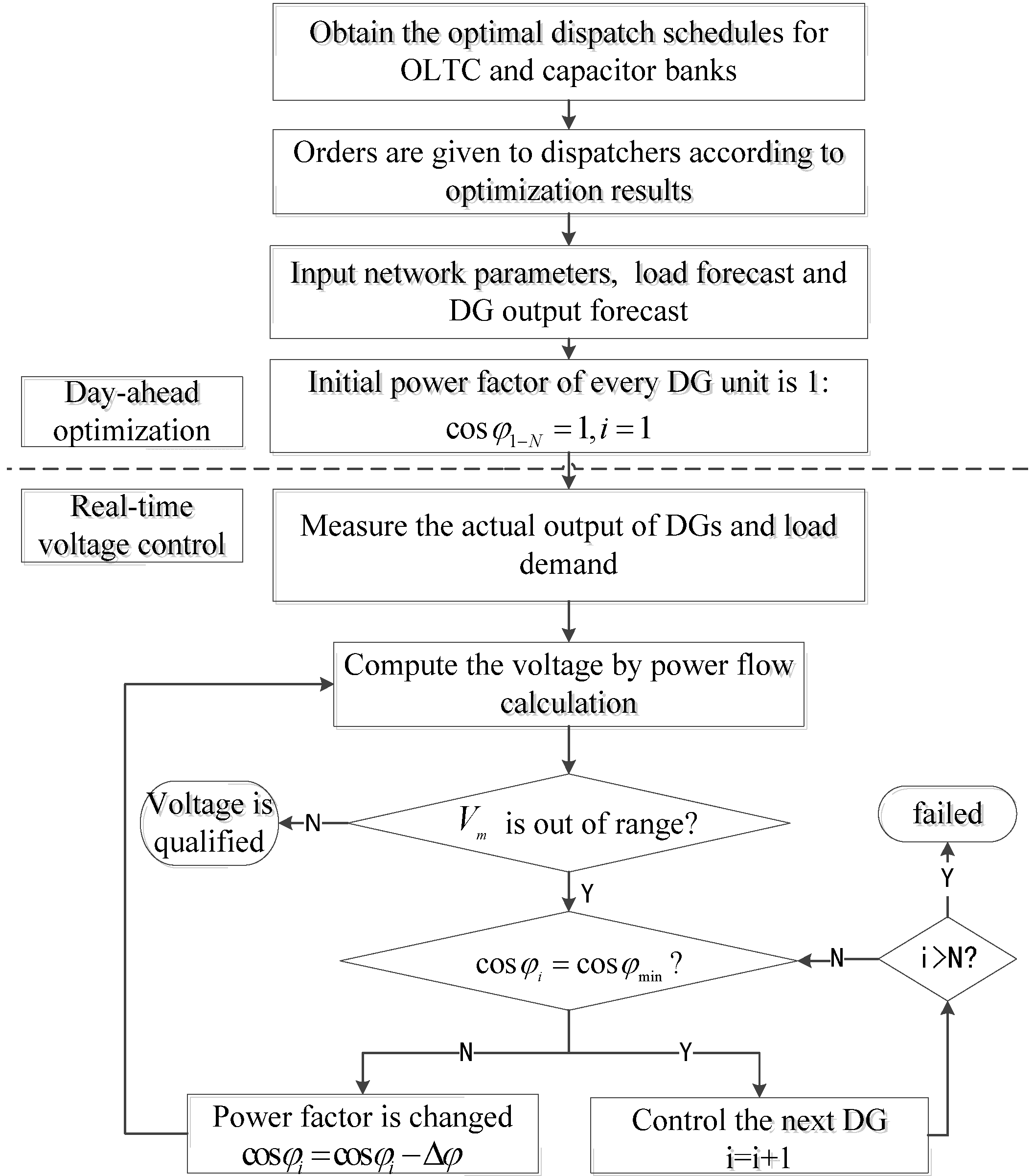
Control Strategy

To make the system more complete, this paper involves day-ahead optimization in decentralized voltage control system. The strategy is divided into day-ahead and real-time scale.

Day-ahead control adopts static optimization method. Based on load forecast and DG output prediction, the upper and lower voltage limits of OLTC and operation voltage of secondary capacitor in substation are computed [22]. After considering operation times, the results of optimization are sent down to dispatchers.

Real-time control adopts decentralized voltage control mode. The dynamic adjustment features of DG can be used to adjust the power factor of generator. Prediction deviations of load and coming water volume can be balanced. Both the day-ahead and real-time control can be achieved without communications. Thus, this decentralized voltage control system needs no communication systems.

To make it clear, the simulation process of this strategy is shown in Figure 1:

• Day-ahead optimization: Make a plan for the distribution network according to the data of typical day; and obtain the action sequence of OLTC, capacitor banks and other devices based on the results of optimization.
• Real-time decentralized voltage control: According to the stochastic models of DG generation and load, start up the voltage control system when voltage of measured node exceeds limits and adjust power factor of DGs successively for under-excited operation.
• Stop voltage control operation when the power factor of the last DG unit reaches cosϕ_min (capacitive) but voltage remains unqualified, which means this voltage control strategy unable to adjust the voltage to normal level.

2.2.3. Centralized Voltage Control System

Centralized voltage control is the most effective way to manage and control the operation of the whole ADS. With the development of communication technology, SCADA (Supervisory Control And Data Acquisition)-centered centralized voltage control can optimize operation based on global information.

(1)

Characteristics of the Method

This method is based on optimization theory. Thus, it can make full use of various voltage control devices to regulate globally, which is able to achieve overall optimization. However, the application of centralized control strategies to the existing networks faces several drawbacks: in addition to the heavy investments necessary for devices and control systems, all centralized approaches require a highly reliable communication channel through the overall distribution network [23].

(2)

Economical Model

Centralized voltage control system is composed of Active Distribution Network Management System (ADMS), area coordination controller and locally automatic controller [24]. After analyzing its economic characteristics, the construction cost of the voltage control system composes ADMS cost, area coordination controller cost, locally automatic controller cost and its communication system construction cost. It can be described as follows:

$$C_{vo.ce}=C_{ADMS}+C_{area}+C_{local}+C_{tx}$$

(3)

where C_vo.de is the construction cost of centralized voltage control system, C_ADMS is the ADMS cost, C_area is the area coordination controller cost, C_local is the cost of locally automatic controller, and C_tx is the construction cost of communication system, which is illustrated in Equation (2).

(3)

Control Strategy

From the perspective of mathematics, centralized voltage control by optimization is a multi-objective non-linear programming problem [25], which can be described as follows:

$$\{\begin{array}{c}\min f(x,u_d,u_c)\\ g(x,u_d,u_c)=0\\ h(x,u_d,u_c)\le 0\end{array}$$

(4)

where u_d is discrete control variable, x is dependent variable that can only be controlled indirectly, and u_c is continuous control variable. Usually, dependent variable x is node voltage or angle. Discrete control variable u_d is switching variable such as position of taps, parallel capacitor and reactor. Continuous control variable u_c is the output of DGs. Objective function is network losses minimization in consideration of voltage quality and other economic indexes. It can be illustrated with Interior Point Method:

$$\min f(x,u_d,u_c)={\displaystyle \sum _{i=1}^N[P_{LOSS}+\lambda {\displaystyle \sum _{j=1}^n{(\frac{\Delta V_j}{V_{j\max }-V_{j\min }})}^2}]}$$

(5)

Equality constraints are power flow equations of every node. Inequality constraints include physical constraints of network components and capacity constraints of controllable resources: voltage within the statutory limits; active power and reactive power constraints of controllable resources; and transformer ratio constraint.

3. Capacity Optimization of DG Considering Voltage Control

The connection of DGs is considered as a solution for environmental pollution, global warming and the rapid depletion of fossil fuels. However, the high penetration of DGs could cause unexpected voltage variation, which is a significant constraint for increasing the share of sustainable sources. By voltage regulation ancillary service with DGs involved, it could avoid the DG units’ disconnections due to the infringement of voltage regulatory limits as much as possible [26]. Therefore, ADS planning should not only keep cost efficient but also maximize DG generation capacity with voltage acceptable. The control ability, demand on communication system and cost of different voltage control system are different. Therefore, besides capacity and location of DGs, decision variables should also include the category of voltage control system.

3.1. DGs Capacity Optimization Model

3.1.1. Objective Functions

On the one hand, considering the profits of DNOs, economy should be considered in ADS planning. On the other hand, generation capacity of DGs should be as large as possible with voltage acceptable. Therefore, this paper takes minimal comprehensive cost and maximal clean energy generation ratio as objectives. DGs capacity optimization model with active voltage control is solved.

Objective Function 1: Minimizing Comprehensive Cost

Comprehensive cost brought to DNOs should be fully considered, which should be as low as possible. Annual comprehensive cost of DG is comprised of construction cost and operation cost. Construction cost includes connection cost of DG units and construction cost of voltage control systems. The main characteristics of DGs project are its high construction cost in prophase and low maintenance cost in operation. Therefore, power losses cost is the only factor considered in the operation cost [27]. Then the following equations illustrate the objective function [28].

$$\{\begin{array}{l}\begin{array}{c}\begin{array}{c}\begin{array}{c}\begin{array}{c}\begin{array}{c}\begin{array}{c}\begin{array}{c}\begin{array}{cc}\min C=C_{co}+C_{op}& \begin{array}{}\end{array}\end{array}\end{array}\end{array}\end{array}\end{array}\end{array}\end{array}\end{array}\\ C_{co}={\displaystyle \sum _{i=1}^{N_{DG}}\frac{C_{i.tr}\cdot \alpha }{1-{\left(1+\alpha \right)}^{-Tl}}}+x_s\frac{C_{vo.de}\cdot \alpha }{1-{\left(1+\alpha \right)}^{-T_{de}}}+(1-x_s)\frac{C_{vo.ce}\cdot \alpha }{1-{\left(1+\alpha \right)}^{-T_{ce}}}\\ C_{op}={\displaystyle \underset{0}{\overset{T}{\int }}\Delta }{P}_{loss}^{t}dt\cdot \lambda \begin{array}{c}\begin{array}{c}\begin{array}{c}\begin{array}{c}\begin{array}{c}\begin{array}{c}\begin{array}{c}\begin{array}{c}\begin{array}{}\end{array}\end{array}\end{array}\end{array}\end{array}\end{array}\end{array}\end{array}\end{array}\\ \begin{array}{c}\begin{array}{c}\begin{array}{c}\begin{array}{c}\begin{array}{c}\begin{array}{c}{x}_s\in \left\{\begin{array}{ccc}0& ，& 1\end{array}\right\}\begin{array}{c}\begin{array}{c}\begin{array}{c}\begin{array}{}\end{array}\end{array}\end{array}\end{array}\end{array}\end{array}\end{array}\end{array}\end{array}\end{array}\end{array}$$

(6)

where C is annual comprehensive cost; C_co is discounted construction cost, C_op is operation cost; C_i.tr is the connection cost of the ith DG unit or means DGs’ newly-built lines cost; N_DG is the number of DGs; Tl, T_de and T_ce are the life of newly built lines, decentralized and centralized voltage control systems, respectively; α stands for bank interest rates; C_vo.de is the construction cost of decentralized voltage control system, which is shown in Equation (1); C_vo.ce is the construction cost of centralized voltage control system, which is shown in Equation (3); x_s is a binary variable determining the category of control system; Δ$P_{loss}^t$ is the total network losses at time t; T is the total time of dispatch; and λ is residential electricity prices.

Objective Function 2: Maximizing Clean Energy Generation Ratio

If the capacity of DGs is overlarge, it may cause voltage unacceptable and out of control. Therefore, when optimizing the capacity of DGs, the actual amount of DG output should be increased as much as possible on the basis of the existing voltage control system, namely to maximize the clean energy generation ratio. According to the definition of clean energy generation ratio in [29], this objective function can be written as:

$$\mathrm{m}\mathrm{a}\mathrm{x}\xi =\frac{{\displaystyle \underset{0}{\overset{T}{\int }}{\displaystyle \sum _{n=1}^{N_G}{P}_{DGn}(t)dt}}}{{\displaystyle \underset{0}{\overset{T}{\int }}{\displaystyle \sum _{m=1}^N{P}_{Lm}(t)dt+{\displaystyle \underset{0}{\overset{T}{\int }}{\displaystyle \sum _{j=1}^{N_B}{P_j}^{loss}(t)}}}}dt}$$

(7)

where ξ is the ratio of clean energy generation, which is the ratio of DGs output to the sum of active load and network losses, and represents the utilization ratio of DGs. T is the total time of dispatch. The dispatching interval is 15 minutes. N_G is the number of DGs, P_DGn(t) is the output of the nth DG at the time of t, N is the total number of nodes, P_Lm(t) is the active load of node m at the time of t, N_B is the total number of distribution network branches, and $P_j^{loss}(\mathrm{t})$ is the total real power losses on branch j at the time of t.

3.1.2. Constraints

Constraint 1: Constraints of Voltage Qualified Rate

Since the output of most DGs is influenced by environment, being intermittent may cause voltage fluctuations. In order to ensure power quality after DG connected to the grid, it is required that voltage qualified rate meet certain requirements after on-line voltage control.

$$\begin{array}{l}{\eta }_{\mathrm{t}}\ge \delta ，{\eta }_{\mathrm{t}}=\frac{{\displaystyle \sum _{i\in i_G,N_i\in N}{N}_i}}{{\displaystyle \sum N}}\\ feasibleregion:i_G=\left\{i|U_{\min }\le U_i\le U_{\max }\right\}\end{array}$$

(8)

where η_t is the voltage qualified rate at time t, δ is the lower limit of voltage qualified rate, N is measured node at time t, N_i is the node in feasible region, U_i is voltage of node i, and U_min and U_max are the lower and upper limits of voltage, respectively.

Constraint 2: Constraints of DGs’ Annual Comprehensive Cost

Considering the profits of DNOs, DGs’ annual comprehensive cost is asked to be acceptable.

$$C_{\min }\le C\le C_{\max }$$

(9)

where C_min and C_max are the lower and upper limit of comprehensive cost, respectively.

Constraint 3: Constraints of Power Flow Equations

$$\{\begin{array}{c}{P_i}^t+{P_{iDG}}^t-{P_{Li}}^t-{U_i}^t{\displaystyle \sum _{j=1}^n{U_j}^t}(G_{ij}\cos {\theta }_{ij}+B_{ij}\sin {\theta }_{ij})=0\\ {Q_i}^t+{Q_{iDG}}^t-{Q_{Li}}^t-{U_i}^t{\displaystyle \sum _{j=1}^n{U_j}^t}(G_{ij}\sin {\theta }_{ij}-B_{ij}\cos {\theta }_{ij})=0\end{array}$$

(10)

where n is the number of nodes, $P_i^t$, $P_{iDG}^t$, $P_{Li}^t$, $Q_i^t$, $Q_{iDG}^t$, $Q_{Li}^t$, and $U_i^t$ are active power output of the main source, active power output of DG, active power demand, reactive power output of infinite system, reactive power output of DG, reactive power demand, and voltage of node i at time t, respectively. G_ij, B_ij and θ_ij are the conductance, susceptance and voltage phase angle difference between node i and node j.

Constraint 4: Constraints of DG Capacity

$$\{\begin{array}{l}\begin{array}{l}\begin{array}{c}{\omega }_{\min }^{DG}\le {\omega }_i^{DG}\le {\omega }_{\max }^{DG}\end{array}\\ 0\le {P_{iDG}}^t\le {{\delta }_{iDG}}^t\begin{array}{cc},& {{\delta }_{iDG}}^t={\mu }_t{\omega }_i^{DG}\end{array}\\ Q_{DG\min }\le {Q_{iDG}}^t\le Q_{DG\max }\end{array}\\ \begin{array}{c}\begin{array}{cc}\forall t\in T,\forall i\in N_{DG}& \begin{array}{c}\begin{array}{c}\begin{array}{}\end{array}\end{array}\end{array}\end{array}\end{array}\end{array}$$

(11)

where ${\omega }_{\min }^{DG}$ and ${\omega }_{\max }^{DG}$ are the upper and lower limits of DG installed capacity, ${\omega }_i^{DG}$ is the installed capacity of the ith DG unit, $P_{iDG}^t$ and $Q_{iDG}^t$ are active power and reactive power of the ith DG in t period, respectively, ${\delta }_{iDG}^t$ is the maximal available DG active power, μ_t is the efficiency of DG unit in t period, and $Q_{DG\min }$ and $Q_{DG\max }$ represent the maximum value of reactive power that the converter is able to absorb and/or inject into distribution network, respectively.

3.2. Multi-Objective Differential Evolution Algorithm

With two objective functions, DGs capacity optimization is a multi-objective problem. However, to solve the multi-objective optimization problems, it needs to meet two or more objectives. Sometimes the multiple goals might contradict each other. Therefore, in solving multi-objective optimization problems, Pareto solution set is usually used. Here, a new intelligent optimization algorithm called differential evolution algorithm (DE), based on population optimization is used. This algorithm has faster convergence rate, fewer adjustable parameters, simple operation and strong robustness [30]. Similar to the standard DE, MODE also includes population initialization, crossover, mutation, selection and other operations. However, being different from DE just based on objective function value, population evolution of MODE is based on the fast non-dominated sorting and the calculation of crowding.

(1)

Population Initialization

Using the classic uniform random initialization method:

$$x_{ij}^0=x_j^L+rand\cdot (x_j^U-x_j^L)$$

(12)

where $x_{ij}^0$ is dimension j of initial individual i. rand is uniformly distributed random number between [0,1]. $x_j^U$ and $x_j^L$ are the upper and lower limits of variable j, respectively. j = 1, 2, ..., D. D is the dimension of the optimization issues.

(2)

Mutation Operation

When the difference vector is added to another individual vector selected randomly, the mutated vector is generated. For each target vector $x_i^t$, the mutation operation is shown in Equation (13).

$${v_i}^{t+1}={x^t}_{r3}+F\cdot ({x^t}_{r1}-{x^t}_{r2})$$

(13)

where r₁, r₂, r₃∊{1, 2, …, NP} are different integers, and r₁, r₂, r₃ are different from current target vector index i. Thus, the size of population NP ≥ 4. F is a scaling factor.

(3)

Crossover Operation

For target vector individual $x_i^t$, it will go on crossover operation with the mutated vector $u_i^{t+1}$, generating trial individuals $u_i^{t+1}$. To ensure the evolution of individual $x_i^t$ by random selection, there is at least one bit of $u_i^{t+1}$ that is contributed by $v_i^{t+1}$. As for other bits, crossover probability factor CR can determine which bit of $u_i^{t+1}$ is contributed by $x_i^t$. The crossover equation is shown in Equation (14).

$${u_{ij}}^{t+1}=\{\begin{array}{c}\begin{array}{ccc}{v_{ij}}^{t+1}\begin{array}{cc},& rand(j)\le CR\end{array}& or& j=randn(i)\end{array}\\ \begin{array}{ccc}{x_{ij}}^t\begin{array}{cc},& rand(j)>CR\end{array}& and& j\ne randn(i)\end{array}\end{array}$$

(14)

where rand(j) ∊ [0,1] is uniformly distributed random number, randn(i) ∊ [1, 2, …, D] is dimension variable index selected randomly, which ensures that at least one dimension variable of trial vector is contributed by the mutated vector.

(4)

Selection Operation

In accordance with a certain strategy, select individuals from parent generation to second generation.

Using a search strategy called “greedy”, the test subject $u_i^{t+1}$ is competed with $x_i^t$. When the adaptation degree of $u_i^{t+1}$ is better than $x_i^t$, $u_i^{t+1}$ can be selected as second generation. Otherwise, $x_i^t$ is selected directly as second generation. Taking the minimal optimization as an example, the equation for selection operation is as follow:

$${x_i}^{t+1}=\{\begin{array}{c}\begin{array}{cc}{u_i}^{t+1},& f({u_i}^{t+1})<f({x_i}^t)\end{array}\\ \begin{array}{cc}{x_i}^t,& f({u_i}^{t+1})\ge f({x_i}^t)\end{array}\end{array}$$

(15)

(5)

Non-Dominated Ranking

The individuals of population are ranked based on non-dominated relationship. A fast non-dominated ranking strategy of typical NSGA-II is used in the case.

(6)

Calculation of Congestion Degree

When new population is generated, usually individuals of high level and small aggregation density are reserved to participate in evolution.

(7)

Shear Operation

After adding every individual of fronts F₁–F_j to the new offspring in turn, if the number exceeds N, they are ranked according to congestion degree. According to the distance, add individuals selected from F_j to the new offspring until the number of individual reaches N.

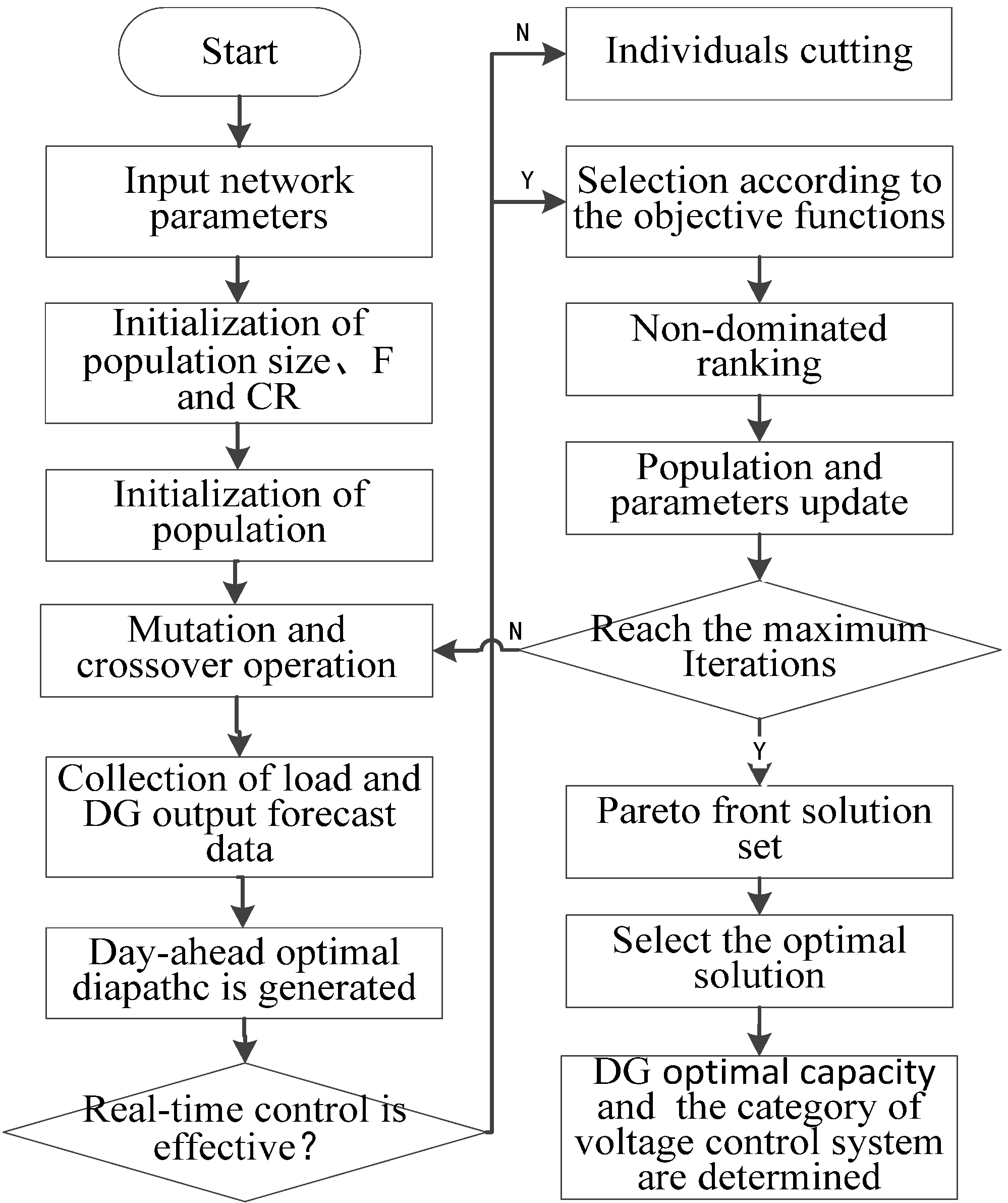
3.3. Optimization Based on Multi-Objective Differential Evolution Algorithm

The flow chart of sizing optimization of DGs considering active voltage control strategy is depicted in Figure 2:

Specific steps are as follows:

• Input the network parameters, initialize the parameters and population, and then conduct the mutation and crossover operations.
• According to the data of typical day, determine the day-ahead optimal dispatch schedule. According to the actual load and output of DG, simulate the real-time voltage regulation with DG participation.
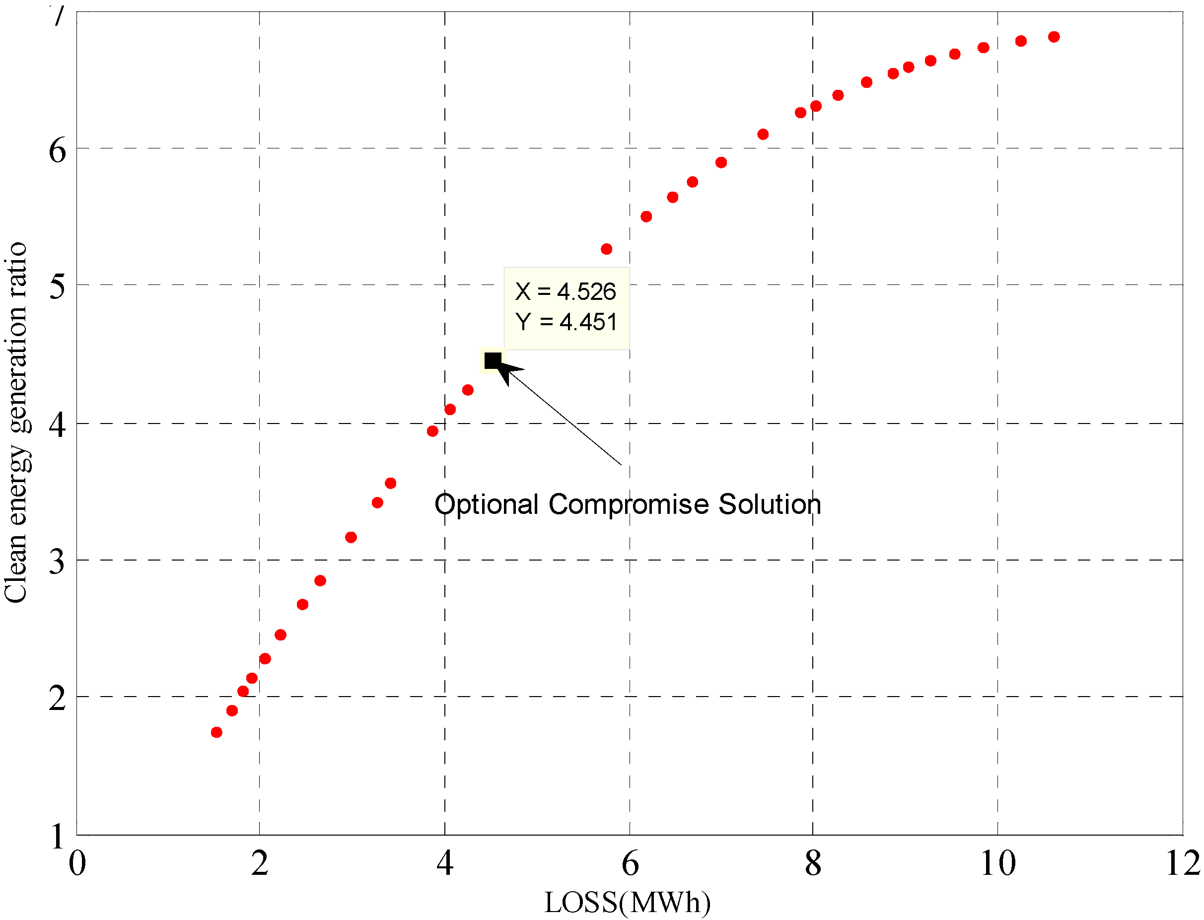
• Taking minimal DGs’ comprehensive cost and maximal clean energy generation ratio as multi-objective functions and voltage qualified rate as constraint, the optimal compromise solution is solved by intelligent algorithm, and then the most appropriate DG capacity is selected.

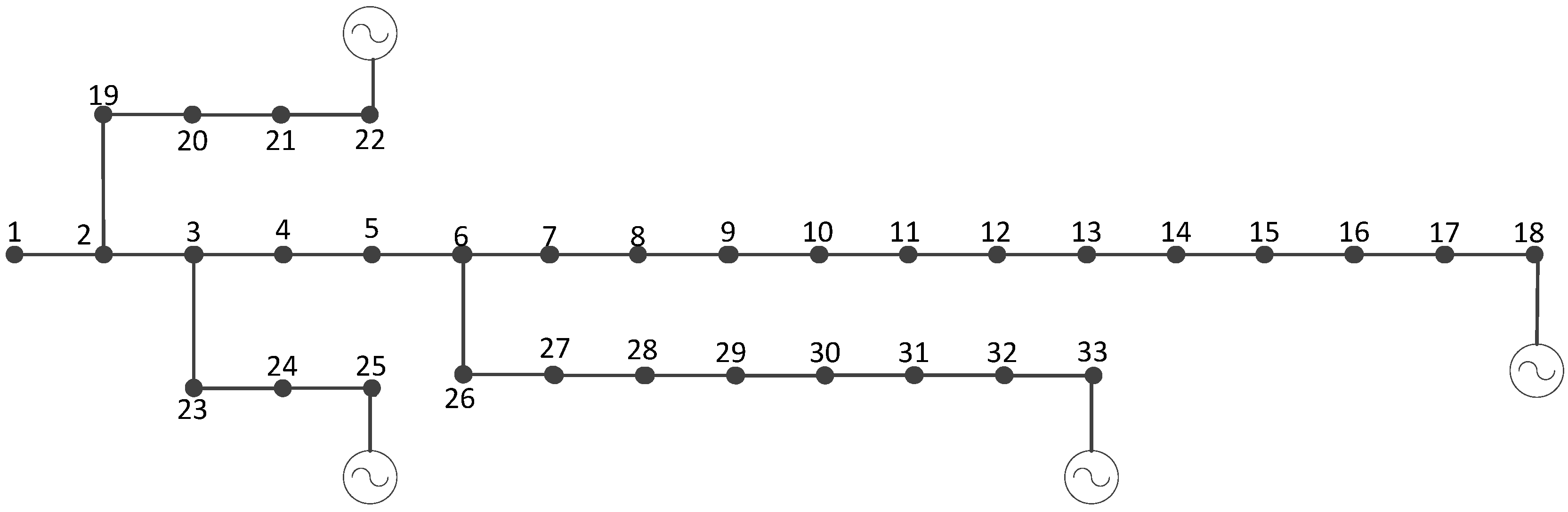
4. Case Study

The simulation is carried on IEEE-33 system, which is a 12.66 kV radial distribution system. The system has one supply point and 32 nodes. The total substation loads of the initial configuration are 3.715 MW and 2.3 Mvar. More parameters of the system can be found in [31]. In renewable energies, SHP is the most widely used and flexible for power generation in China, especially in remote areas. According to the situation of actual installation described in [32], four small hydropower plants are connected at different positions along the feeder. The gird topology and installed SHP plants are shown in Figure 3. The parameter values used in MODE are as follows [33]: Population size is 100, the maximum number of iterations is 2000, the maximum and minimum factor ratios are 0.9 and 0.1, respectively, and the maximum and minimum cross ratios are 0.8 and 0.3, respectively.

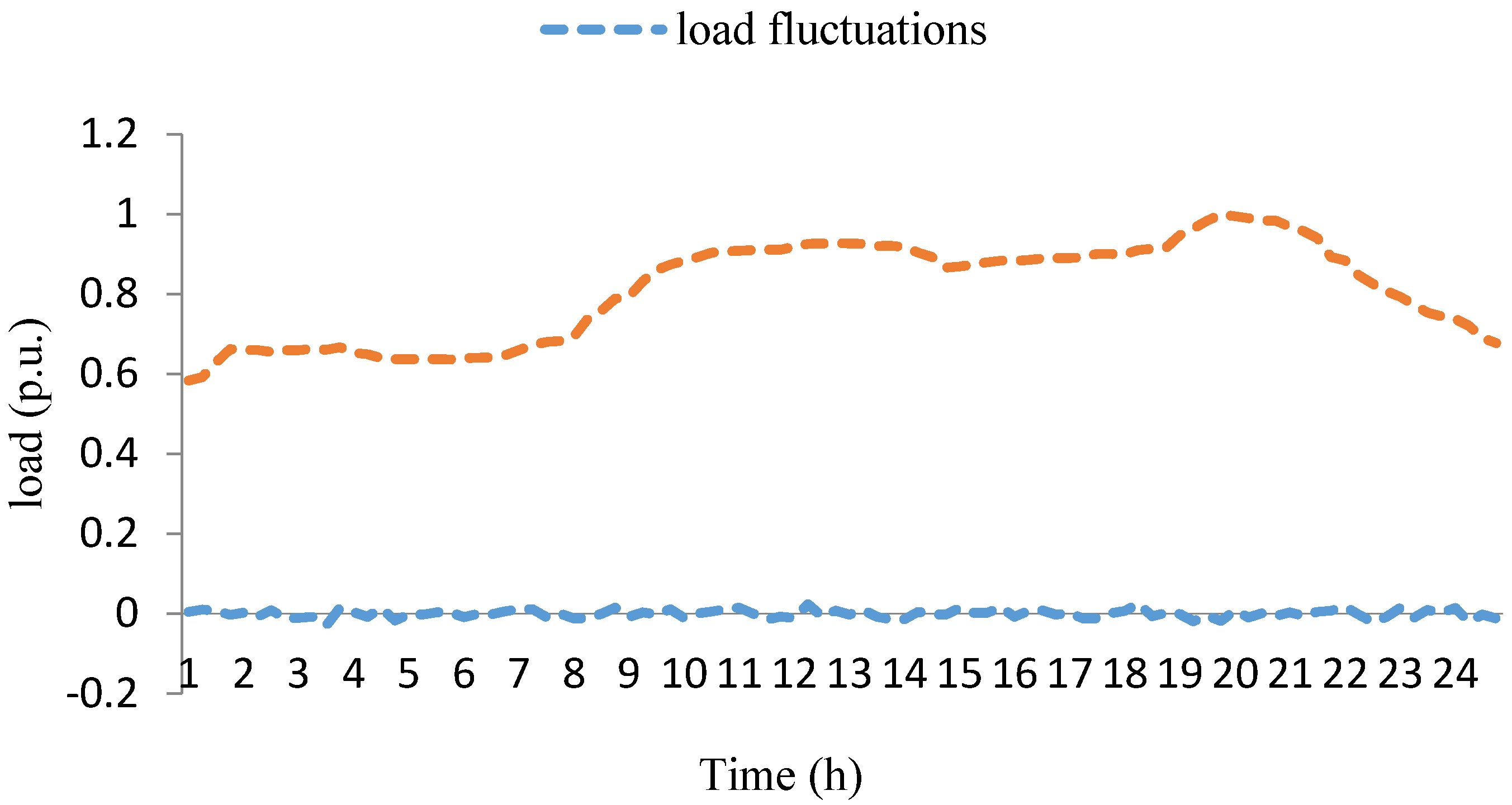
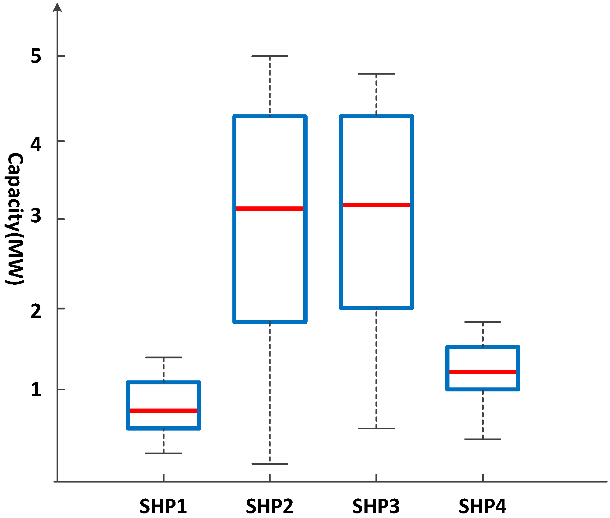
4.1. Stochastic Modeling of SHP Generation and Load

The generated power of SHP plants depends on the specific weight of the water, the river inflow, the height of the waterfall and the efficiencies of the electric generator [34]. However, the river inflow is modeled as a stochastic process, and rainfall has hysteresis and cumulative effects [35]. It is difficult to describe the stochastic distribution of SHP generation by specific probability model. Water resource is usually abundant in wet season, which makes the power generation of SHP plants very large. In this case, the system voltage tends to be higher than the statutory limits, which is the focus of our study. Therefore, the output characteristics of SHP in wet season are analyzed here. In wet season, the SHP units usually operate at closely to the rated condition with the maximal efficiency approaching 85% [36]. The efficiency of SHP plant is defined as follows:

$${P_{SHP}}^t={\mu }^t{\omega }_{SHP}$$

(16)

where μ^t is efficiency of SHP plant during t period, ω_SHP is the installed capacity of SHP plant, $P_{SHP}^t$ is active power of SHP plant during t period. The daily output of SHP plant follows Gamma distribution [35]. Its probability distribution is illustrated as follows:

$$f(P_{SHP})=\frac{1}{b^a\mathsf{\Gamma }(a)}{P_{SHP}}^{a-1}{e}^{-\frac{P_{SHP}}{b}}$$

(17)

where P_SHP is active power of SHP plant, Γ(·) is Gamma equation, a = 0.1055, b = −0.0102.

As for the stochastic modeling of load, it can be illustrated as follows:

$$\begin{array}{l}{P}_{load}^t=P_0^t+{\alpha }^t\\ Q_{load}^t=Q_0^t+{\beta }^t\end{array}$$

(18)

where $P_{load}^t$ and $Q_{load}^t$ are the load at time t, $P_0^t$ and $Q_0^t$ are the basic load at time t which can be obtained by the data of typical day considering the daily variation characteristics of load, and α^t and β^t are the possible fluctuations of load, which follow Normal distribution [35]. Load data on the typical day are shown in Figure 4.

In the simulation, parameters of the day-ahead optimal dispatch schedule adopt the parameters of the typical day. To give consideration to both accuracy and the amount of calculation, the typical day is used to represent the operation of the grid throughout the year [37]. The initial power factor of every SHP is 1.0.

4.2. Simulation Analysis of Multi-Objective Functions Capacity Optimization

In this scenario, SHP plants are mostly located in remote mountainous area. On the one hand, it is very difficult to lay wire communication lines. On the other hand, wireless communication is lack of stability and less effective. The centralized control method needs great additional investment for the construction of a control central and some communication infrastructures. The cost of communication system here is very high. Centralized voltage control scheme is unsuitable to adopt, which needs global information. Thus, centralized voltage control is abandoned and decentralized voltage control is adopted, which needs no communication system.

To make the problem simple, in simulation, minimal network losses and maximal clean energy generation ratio are taken as the multi-objective functions. The Pareto front solution set solved by MODE is shown in Figure 5.

All of the solutions presented by the Pareto fronts are valid thresholds for the optimization problem [38]. The choice of one of them represents the optimal tradeoff between active losses minimization and renewable energy usage maximization. Considering that the network losses should be within acceptable range, the optimal compromise solution is selected. Results show that the optimal total capacity of SHPs is 7.8261 MW. The capacities of SHPs connected to node 18, node 22, node 25 and node 33 are 0.6682 MW, 2.7836 MW, 2.8936 MW and 1.4807 MW, respectively. Voltage qualified rate at any monitoring time during the day is 1. Network losses of the whole day are 4.526 MWh, and network losses rate is 3.29%. Clean energy generation ratio is 4.451. Power flow runs reversely back in this scenario. The voltage regulation system is started, but not frequently. Power losses during 24 h on typical day are shown in

Table 1. Power losses profile based on optimal capacity considering voltage control.

Time	Loss (MWh)	Time	Loss (MWh)	Time	Loss (MWh)	Time	Loss (MWh)
1	0.099	7	0.184	13	0.285	19	0.159
2	0.107	8	0.210	14	0.306	20	0.145
3	0.114	9	0.225	15	0.327	21	0.114
4	0.120	10	0.260	16	0.311	22	0.103
5	0.135	11	0.263	17	0.237	23	0.091
6	0.133	12	0.269	18	0.181	24	0.091

.

Average electricity sales price in a certain region is 0.48 RMB/kWh. To accept the newly-built four SHP plants, electricity lines use LGJ-185. The total length of lines is 30 km. The unit price is RMB 130 million per km. The Comprehensive unit prices of communication equipment in distribution network are shown in

Table 2. Comprehensive unit prices (k RMB) of communication equipment in distribution network

No.	Equipment Type	Equipment	Unit	Unit Prices
1	Connection fiber	Fiber and auxiliary devices	km	20
2	Fiber communication	EPON-OLT	set	150
3		EPON-ONU	set	7
4	Public wireless communication	GPRS Terminal	set	3
5	Network management	Network management equipment	set	2000
6	Construction control cost	Include project management cost, investigation and design fee, etc.		2000

Note: The unit k RMB means thousand RMB.

[39].

To show the reduction of total cost, a comparison of different study cases is conducted when the centralized voltage control approach is used instead. The capacities of SHPs connected to node 18, node 22, node 25 and node 33 are 0.6682 MW, 2.7836 MW, 2.8936 MW and 1.4807 MW, respectively. Results show that, with centralized voltage control, voltage qualified rate at any monitoring time during the day is 1. The network losses of the whole day are 4.0274 MWh and the network losses rate is 2.364%. To analyze the costs clearly,

Table 3. Cost analysis of the optimal scheme with different control systems.

The Optimal Scheme		Decentralized Voltage Control	Centralized Voltage Control
Total capacity of SHPs (MW)		7.8261	7.8261
Construction cost (k RMB)	Newly-built lines fee	39,000	39,000
	Construction cost of Voltage control system	500	5800
	Construction cost of communication system	0	50,000
Operation cost (k RMB)		1425.3	1253.5
Comprehensive cost (k RMB)		40,925.3	96,053.5

shows the result of the optimal scheme.

Compared with the centralized method, decentralized voltage control has a great reduction in the total cost, especially in the part of the construction cost of communication system. Although the centralized approach reduces the operation cost, it is too small to ignore compared to the cost of the control system.

4.3. Influence of Voltage Control System on DG Capacity

To analyze the influence of voltage control system on DG capacity, the optimal capacity of DGs without voltage control can be calculated in the same way. In the process of simulation, active voltage control is abandoned. Results show that the optimal total capacity of SHPs is 6.397 MW. The capacities of SHPs connected to node 18, node 22, node 25 and node 33 are 0.5397 MW, 2.2384 MW, 2.7493 MW and 0.8696 MW, respectively. Network losses of the whole day are 3.1243 MWh, and network losses rate is 1.46%. Clean energy generation ratio is 3.6424.

From

Table 4. Influence of voltage control system on DG capacity.

Comparisons	With Voltage Control	Without Voltage Control
Optimal capacity (MW)	7.8261	6.397
Clean energy generation ratio	4.451	3.6424
Network losses rate (%)	3.29	2.16
Voltage (voltage qualified rate)	Acceptable (100%)	Unacceptable (83.33%)

, with the help of improving the voltage profile, voltage control system increases the capacity of DGs. Although network losses increase either, network losses rate is still acceptable. Meanwhile, the construction cost of centralized voltage control is regarded as infinite compared with decentralized.

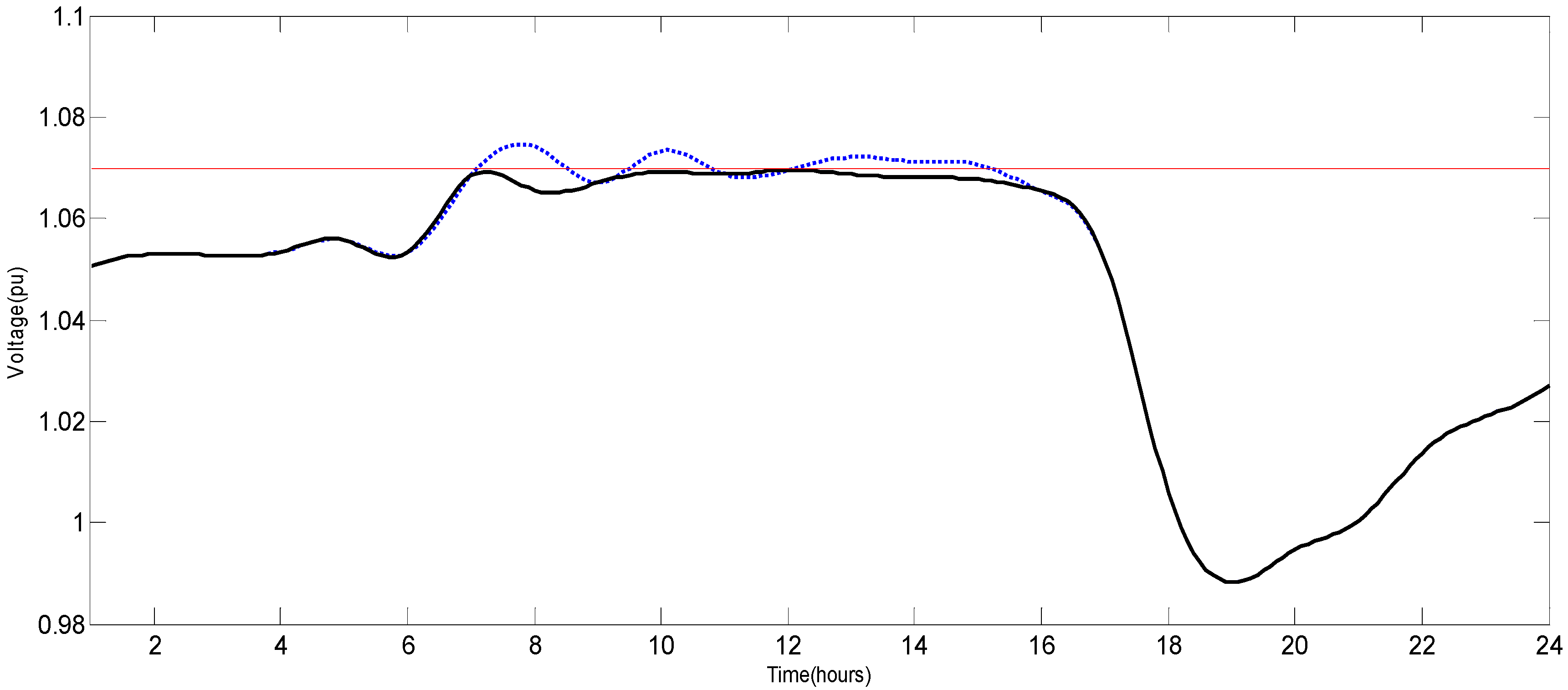
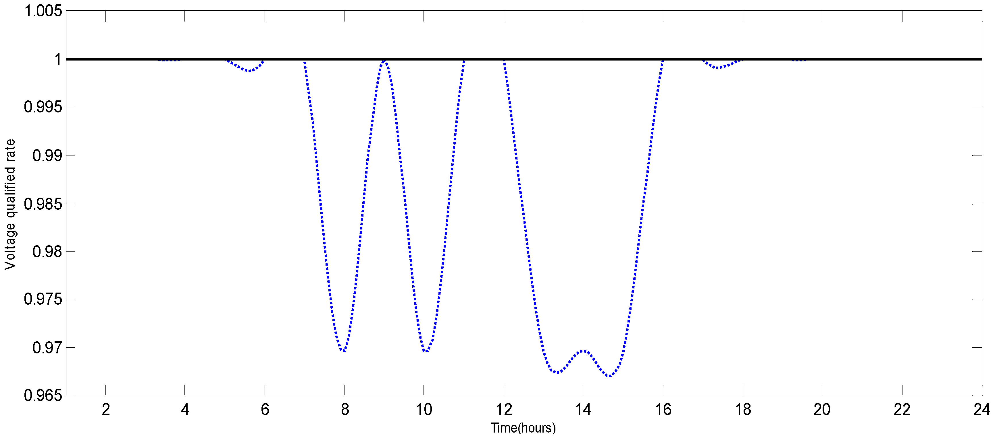
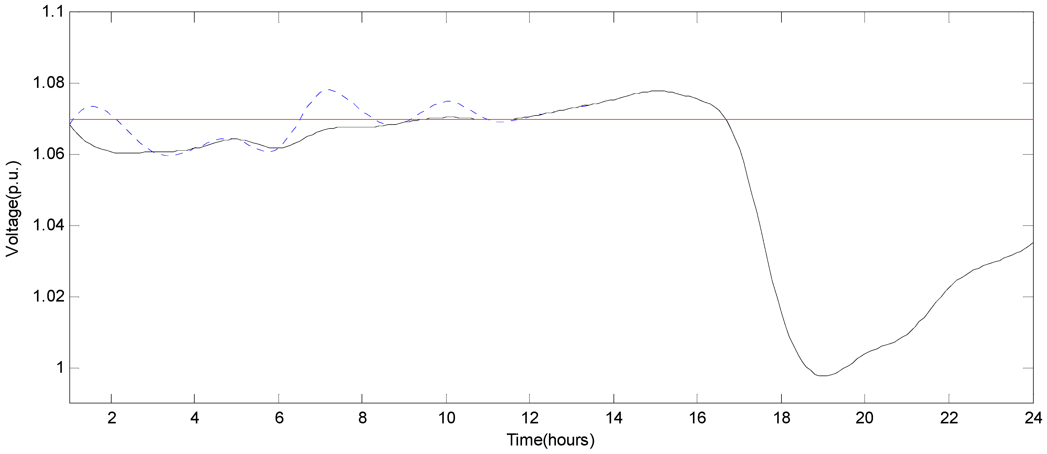
4.4. The Control Effect of Proposed Voltage Control Method

To prove the ability of the proposed decentralized voltage control method, a further simulation was carried out with daily variations of loads and generations.

From Figure 6 and Figure 7, the proposed voltage control strategy reduces the voltage rise effectively and the voltage profile rapidly drops as a consequence. The effect of proposed voltage control method is illustrated. Once the voltage of the monitoring node exceeds specified limits, the voltage control system begins. It is confirmed that the proposed technique contributes to voltage adjustment. With voltage profile adjusted, larger DGs are permitted to be connected to distribution networks. However, the ability to control voltage is limited with the voltage profile worsen as shown in Figure 8. In this case, the voltage at, or around, 4:00 p.m. is still over the limit with control action, as the algorithm cannot find a valid solution.

4.5. Relevance between the Capacity of DG and Load, Circuit Structure

According to the calculation results, distribution of SHP capacity is shown in Figure 9, where SHP 1, SHP 2, SHP 3 and SHP 4 stand for SHP plants connected to node 18, node 22, node 25 and node 33, respectively.

From Figure 8, capacities of SHP 2 and SHP 3 are larger. The reason is that they are at the load center and closer to the system bus with less influence on voltage. As SHP 1 and SHP 4 are far away from the system bus, the load is lighter and the load relevance is weaker, easily making network voltage out of range. Compared to SHP 3, the range of capacity distribution and the maximal achievable capacity of SHP 2 are larger.

5. Conclusions

This study has presented a new ADS planning approach for promoting renewable energy usage and the benefits of DNOs while keeping voltage profile acceptable. Especially, the costs of specific control system and its supporting systems are included in the optimization model, and the effect of voltage control is included in the simulation. Based on the theoretical analysis and simulation results above, this paper draws the following conclusions:

(1)

The cost of control system and its supporting systems are included in the objectives of planning. Therefore, it takes the impacts of control system on the costs of operation and construction into account. The control effect of voltage regulation is included in the simulation. Therefore, the control ability can be verified instead of being estimated roughly. Having made improvements in the above two aspects, the precision of planning can be improved.

(2)

Different control systems have different influences on the planning and operation of the grid. Both the decentralized and centralized approaches can reduce voltage rises and increase the acceptable capacities of DG units to a certain degree, and the effect of the latter is better. However, the centralized approach means a great investment in related costs. With the power grid becoming smarter, more automatic and complicated, the cost of these systems will account for a large share of the total cost. If the cost saving is the priority, adopting the decentralized approach is suggested. If the control effect or DG penetration is the priority, adopting the centralized approach is suggested.

(3)

The proposed approach allows DNOs to obtain benefits by inducing the comprehensive cost and maximizes the usage of renewable energy. The algorithm of MODE can compute the optimal capacity of DG units.

(4)

In the absence of a widespread communication channel, decentralized voltage control method provides an effective solution to mitigate voltage problem. The simulation results show that the proposed voltage control method helps improve voltage to some extent, and DG capacity can be increased by 12.88%.

(5)

Compared with the traditional voltage control methods such as the installation of additional reactive power supply, the proposed voltage control from DGs strategy has more potential. Traditionally, it is difficult to determine the optimal location of reactive power controllers because the configuration of the distribution system may be changed in the future. Furthermore, the setting costs for the installation of additional reactive power compensator is not beneficial for power utilities. The case study proves the effectiveness and advantages of the proposed method.

(6)

The optimal capacity of DG near the system bus is relatively larger. The optimal capacity of DG near heavy loads and with better load relevance is also relatively larger.

References

- Senjyu, T.; Miyazato, Y.; Yona, A.; Urasaki, N.; Funabashi, T. Optimal distribution voltage control and coordination with distributed generation. IEEE Trans. Power Deliv. 2008, 23, 1236–1242. [Google Scholar] [CrossRef]
- Xu, X.; Huang, Y.; Liu, C.; Wang, W.; Wang, Y.L. Influence of Distributed Photovoltaic Generation on Voltage in Distribution Network and Solution of Voltage Beyond Limits. Power Sys. Tech. 2010, 10, 140–146. [Google Scholar]
- NHadjsaid, N.; Canard, J.; Dumas, F. Dispersed generation impact on distribution networks. IEEE Comput. Appl. Power Mag. 1999, 12, 22–28. [Google Scholar] [CrossRef]
- Georgilakis, P.S.; Hatziargyriou, N.D. Optimal distributed generation placement in power distribution networks: Models, methods, and future research. IEEE Trans. Power Syst. 2013, 28, 3420–3428. [Google Scholar] [CrossRef]
- Georgilakis, P.S.; Hatziargyriou, N.D. A review of power distribution planning in the modern power systems era: Models, methods and future research. Elec. Power Syst. Res. 2015, 121, 89–100. [Google Scholar] [CrossRef]
- Kashem, M.A.; Le, A.D.T.; Negnevitsky, M.; Ledwich, G. Distributed generation for minimization of power losses in distribution systems. In Proceedings of the IEEE Power Engineering Society General Meeting, Montreal, QC, Canada, 18–22 June 2006.
- Evangelopoulos, V.A.; Georgilakis, P.S. Optimal distributed generation placement under uncertainties based on point estimate method embedded genetic algorithm. IEE Proc. Generat. Transm. Distrib. 2014, 8, 389–400. [Google Scholar] [CrossRef]
- Jaganathan, S.; Palaniswami, S. Control of voltage profile with optimal control and placement of distributed generation using the refined bacterial foraging algorithm. J. Vib. Contr. 2014, 20, 2006–2018. [Google Scholar] [CrossRef]
- Li, P.; Zhang, L.; Wang, W.; Yang, X.; Zhao, Y. Application and Analysis of Microgrid. Autom. Electr. Power Syst. 2009, 33, 109–114. [Google Scholar]
- Harrison, G.P.; Wallace, A.R. Optimal power flow evaluation of distribution network capacity for the connection of distributed generation. IEE Proc. Generat. Transm. Distrib. 2005, 152, 115–122. [Google Scholar] [CrossRef]
- Borges, C.L.T.; Martins, V.F. Multistage expansion planning for active distribution networks under demand and distributed generation uncertainties. Int. J. Electr. Power Energ. Syst. 2012, 36, 107–116. [Google Scholar] [CrossRef]
- Zhang, W.; Li, F.; Tolbert, L.M. Review of reactive power planning: Objectives, constraints, and algorithm. IEEE Trans. Power Deliv. 2007, 22, 2177–2186. [Google Scholar] [CrossRef]
- Sridhar, S.; Hahn, A.; Govindarasu, M. Cyber–physical system security for the electric power grid. Pro. IEEE 2012, 100, 210–224. [Google Scholar] [CrossRef]
- Raz, D.; Shavitt, Y. Active networks for efficient distributed network management. IEEE Comm. Mag. 2000, 38, 138–143. [Google Scholar] [CrossRef]
- Puttgen, H.B.; MacGregor, P.R.; Lambert, F.C. Distributed generation: semantic hype or the dawn of a new era. IEEE Power Energy Mag. 2003, 1, 22–29. [Google Scholar] [CrossRef]
- Dugan, R.C.; McGranaghan, M.F.; Beaty, H.W. Electrical Power Systems Quality; McGraw-Hill: New York, NY, USA, 1996. [Google Scholar]
- Hashim, T.J.T.; Mohamed, A.; Shareef, H. A review on voltage control methods for active distribution networks. Electr. Rev. 2012, 88, 304–312. [Google Scholar]
- Conti, S.; Greco, A.M. Active MV distribution network planning coordinated with advanced centralized voltage regulation system. In Proceedings of the 2007 IEEE Lausanne Powertech, Lausanne, Switzerland, 1–5 July 2007.
- Sansawatt, T.; O’Donnell, J.; Ochoa, L.F.; Harrison, G.P. Decentralised voltage control for active distribution networks. In Proceedings of the Universities Power Engineering Conference (UPEC), 2009 Proceedings of the 44th International, Glasgow, UK, 1–4 September 2009.
- Ochoa, L.F.; Harrison, G.P. Minimizing energy losses: Optimal accommodation and smart operation of renewable distributed generation. IEEE Trans. Power Syst. 2011, 26, 198–205. [Google Scholar] [CrossRef]
- Unger, D.; Spitalny, L.; Myrzik, J.M.A. Voltage control by small hydro power plants integrated into a virtual power plant. In Proceedings of the 2012 IEEE Energytech, Cleveland, OI, USA, 29–31 May 2012.
- Golshan, M.E.H.; Arefifar, S.A. Optimal allocation of distributed generation and reactive sources considering tap positions of voltage regulators as control variables. Eur. Trans. Electr. Power 2007, 17, 219–239. [Google Scholar] [CrossRef]
- Farag, H.E.Z.; El-Saadany, E.F. A novel cooperative protocol for distributed voltage control in active distribution systems. IEEE Trans. Power Syst. 2013, 28, 1645–1656. [Google Scholar] [CrossRef]
- Vovos, P.N.; Kiprakis, A.E.; Wallace, A.R.; Harrison, G.P. Centralized and distributed voltage control: Impact on distributed generation penetration. IEEE Trans. Power Syst. 2007, 22, 476–483. [Google Scholar] [CrossRef]
- Kiprakis, A.E.; Wallace, A.R. Maximising energy capture from distributed generators in weak networks. IEE Proc. C Generat. Transm. Distrib. 2004, 151, 611–618. [Google Scholar] [CrossRef]
- Eberly, T.W.; Schaefer, R.C. Voltage versus VAr/power-factor regulation on synchronous generators. IEEE Trans. Ind. Appl. 2002, 38, 1682–1687. [Google Scholar] [CrossRef]
- Jin, Y.X.; Cheng, H.Z.; Yan, J.Y.; Zhang, L. New discrete method for particle swarm optimization and its application in transmission network expansion planning. Elec. Power Syst. Res. 2007, 77, 227–233. [Google Scholar] [CrossRef]
- Liu, W.; Li, Y.; Li, H.; Zhao, T.; Zhang, J. Wind power accommodation capability considering economic constraints for western mountain areas. Electr. Power Auto. Equip. 2014, 34, 19–24. (In Chinese) [Google Scholar]
- Smith, T.C.; Lyshevski, S.E. Clean high-energy density renewable power generation systems with soft-switching sliding mode control laws. In Proceedings of the Decision and Control and European Control Conference (CDC-ECC), 2011 50th IEEE Conference, Orlando, FL, USA, 12–15 December 2011.
- Zhou, Y.; Li, X.; Gao, L. A differential evolution algorithm with intersect mutation operator. Appl. Soft Comput. 2013, 13, 390–401. [Google Scholar] [CrossRef]
- Dharageshwari, K.; Nayanatara, C. Multiobjective optimal placement of multiple distributed generations in IEEE 33 bus radial system using simulated annealing. In Proceedings of the 2015 International Conference on Circuit, Power and Computing Technologies (ICCPCT), CEBU, Philippines, 27–28 March 2015.
- Wijesinghe, A.; Lai, L.L. Small hydro power plant analysis and development. In Proceedings of the 2011 4th International Conference on Electric Utility Deregulation and Restructuring and Power Technologies (DRPT), Weihai, China, 6–9 July 2011.
- Xu, Y.; Zhao, L. A fast multi-objective differential evolutionary algorithm based on sorting of non-dominated solutions. In Proceedings of the 2015 IEEE 14th International Conference on Cognitive Informatics & Cognitive Computing (ICCI*CC), Beijing, China, 6–8 July 2015.
- Laodee, P.; Ketjoy, N. A small hydro-power electricity generation system in Thailand. In Proceedings of the 8th IET International Conference on Advances in Power System Control, Operation and Management (APSCOM), London, UK, 8–11 November 2009.
- Peng, Z.; Wang, X.; Peng, X.; Pan, G. Stochastic Modeling of Small Hydropower Generation Based on Reginonal Synchronism Feature and Its Allowed Penetration Level Evaluation. Water Resour. Power 2015, 33, 171–175. (In Chinese) [Google Scholar]
- Borges, C.L.T.; Pinto, R.J. Small hydro power plants energy availability modeling for generation reliability evaluation. IEEE Trans. Power Syst. 2008, 23, 1125–1135. [Google Scholar] [CrossRef]
- Zeng, B.; Liu, N.; Zhang, Y.; Yang, X.; Zhang, J.; Liu, W. Bi-level Scenario Programming of Active Distribution Network for Promoting Intermittent Distributed Generation Utilization. Trans. China Electrotech. Soc. 2013, 28, 155–163. (In Chinese) [Google Scholar]
- Calderaro, V.; Conio, G.; Galdi, V.; Massa, G.; Piccolo, A. Optimal decentralized voltage control for distribution systems with inverter-based distributed generators. IEEE Trans. Power Syst. 2014, 29, 230–241. [Google Scholar] [CrossRef]
- Dudash, A.; Melvin, W.A., Jr.; Vercellotti, L.C. Distribution Network Communication System Having Branch Connected Repeaters; IFI CLAIMS Patent Services: New Haven, CT, USA, 1981. [Google Scholar]