1. Introduction
As the globalization of the economy accelerated, today’s supply chains span the globe with the unexpected changes in market demands and uncertainties of supply. These changes and uncertainties not only increase risks, but also reduce visibility that, in turn, makes supply chain operations more vulnerable to unforeseen disruptions. A supply chain might suffer from major supply disruptions caused by web server internal errors, storms, strikes, workforce reduction, natural disasters, etc. A supply disruption not only directly affects the supplier, but also results in significant loss to the downstream members of the supply chain (Li et al. [
1]). For example, the earthquake in Japan in 2011 caused Japan’s new vehicle sales in April to be halved, sinking to the lowest monthly tally on record. Sales of cars fell 51 percent from the year before, and market leader Toyota put in the worst performance with a 69 percent drop. That is because domestic auto manufacturers felt the full brunt of the 11 March earthquake, which caused unprecedented disruption to car production. Those natural disasters had exerted some serious effects on supply chain management.
Reflecting growing concerns over supply chain disruptions, supply chain risk management has become an emerging research topic (Kihyun et al. [
2]). Generally, a coordinated decentralized supply chain usually performs better than an uncoordinated one (Chen et al. [
3]). Supply chain contracts could provide its coordination; it can also be called coordination in a decentralized supply chain if and only if the total channel profit of the decentralized supply chain of that contract is equal to the centralized supply chain system. The study of the contract strategy has a significant and practical meaning for the supply chain system; recently, scholars have obtained a series of impressive and practical results in related research fields. Interested readers may refer to Liu and Li [
4], Shin and Benton [
5], Zhou [
6] and Arcelus et al. [
7]. In our paper, we specially consider two kinds of supply chain contracts, wholesale price contracts and buy-back contracts, and implement the two contracts for a three-echelon supply chain in terms of both supply disruption and stochastic demand.
The above observations provide us the motivation for the current work. In this paper, we focus on three areas of research: research on supply disruption, research on the inventory model with substitution and research on the contract in a supply chain with stochastic demand. Integrating supply disruption, the inventory model with substitution and contract coordination into one system is the innovation of the article. This paper intends to answer the following questions:
- (1)
How does the supply disruption impact the integrated performance?
- (2)
How does the dual replacement influence the profit of each member and the total profit of the system?
- (3)
How do the wholesale price contract and buy-back contract coordinate the supply chain system of substitute products?
- (4)
Which contract strategy could make the channel gross profit recovered?
- (5)
How does one decide the buy-back price in order to make the channel gross profit recovered?
To answer these questions, we build a three-echelon supply chain setting in which two suppliers provide the components for a manufacturer; then the manufacturer assembles the products; after having been assembled, the manufacturer provides the products for the retailer, who sells the final products to consumers. When the supplier encounters a supply disruption risk, the manufacturer sends out the order to the spot market immediately and then provides the retailer with substitute products. In this paper, we aim to study the coordinated role of the contract decision on the three-echelon supply chain based on substitute products and how to decide the buy-back price to make the performance under a decentralized decision return to the level of the centralized supply chain.
The contribution of this paper contains four parts. First, we obtain a unique optimal order quantity of the centralized supply chain by analyzing the channel gross profit function. Second, under the decentralized decision, we find that the commonly-used wholesale price contracts cannot coordinate the system, and then, we propose a buy-back contract, which can more efficiently coordinate the system than the former. Third, we explore the effects of supply uncertainty and the substitution behavior of customers on the optimal decision of each member through numerical analysis. Fourth, we also illustrate that the integrated performance of the decentralized system can be maximized through choosing the buy-back parameter by the manufacturer.
The remainder of this paper is organized as follows: In
Section 2, we review the relevant literature.
Section 3 gives us the model description, assumptions and symbols used in the paper.
Section 4 presents the model under centralized decision-making. In
Section 5 and
Section 6, we examine the maximal profit of each member under the decentralized decision in the case of the wholesale price contract and the buy-back contract, respectively, and analyze the impact of contract parameter on the total profit of the decentralized supply chain.
Section 7 demonstrates that the manufacturer makes the supply chain more coordinated through controlling the parameter by using numerical examples. The last section summarizes our research findings and future directions.
2. Literature Review
This paper is closely related to disruption management and supply chain coordination management. We review the literature that is representative and particularly relevant to our study.
A great number of articles on supply chain systems always assumed that supply is reliable, namely the quantity of supply equals the quantity of ordering. However, in real commercial activities, the supply disruption of supply chain upstream enterprises is always inevitable because of the influence from various indefinite factors and risks, such as equipment failures, natural disasters, unexpected social events, etc. Serel [
8] explored an extension of the single-period (newsboy) inventory problem when supply is uncertain. Qi et al. [
9] investigated a continuous-review inventory problem for a retailer who faces random disruptions both internally and externally (from its supplier). Hou et al. [
10] studied a buy-back contract between a buyer and a backup supplier when the buyer’s main supplier experiences disruptions. Sargnt and Qi [
11] studied a continuous-review inventory problem of a two-echelon supply chain with random supply and retailer disruption. There are three approaches to characterize supply uncertainty (He et al. [
12]). In our model, the supplier’s status shows the following two situations: one is the stochastic supply problem, which manifests the random function of ordering quantity; the other is the supply disruption, which means that supply quantity equals zero (Lou et al. [
13]). We can group supply disruption into two general categories: one is that the supplier cannot provide components or products to the manufacturer; the other is that the supply of components or products is disrupted in the course of delivery from supplier to manufacturer (Zhang and Xie [
14]). The two kinds of disruptions are contained in this paper. More relevant literature can be found in He and Zhao [
15] and Shao [
16].
Similar to the current literature on supply chain management, this paper assumes that the demand of goods is random. Market demand of some goods is generally unknown in practice. Although retailer make the decision on the market demand of goods according to the year’s experience of sales and the market database, this still lacks accuracy. Arcelus et al. [
17] studied how a single manufacturer and retailer coordinate through a buy-back contract when market demand is uncertain. Hu et al. [
18] studied a flexible ordering policy among a manufacturer and a supplier with random yield and demand uncertainty. The assumption of random demand is more realistic.
There are some more specialized phenomena in the practical commodity transaction market, i.e., a number of products have a certain substitutability. The degree of substitution depends on the cost performance of the alternatives and the preference of consumers. Bassok et al. [
19] studied a single period multi-product inventory problem with substitution and proportional costs and revenues. Balakrishnan and Geunes [
20] described a dynamic-programming solution method to find the production and substitution quantities that satisfy given multi-period downstream demands at minimum total setup, production, conversion and holding cost. We only consider the unidirectional substitutability between the two goods unless otherwise stated in this paper.
In addition, the management and optimization of the supply chain are the focuses of the industry at present and, hence, are used as a tool to reduce negative environmental influence [
21]; furthermore, they are the most popular research fields, as well. In fact, the essence lies in how to coordinate the profit of each member of the supply chain with the total profit of the whole chain. Pasternack [
22] originally proposed the concept of supply chain contracts. Tsay [
23] pointed out that the wholesale price contract is simple and easy to manage, but coordination between supplier and retailer cannot be realized in general. More research also proved the view above, such as Lariviere [
24], Lariviere and Porteus [
25] and He and Zhao [
15]. Padmanabhan [
26] showed that the buy-back contract could lead to the retailer making an irrational order quantity under fixed market demand. For example, in the clothing industry, the manufacturer buys back part of the unsold products to encourage the retailer to order a large quantity. Yao [
27] discussed the influence of information symmetry and information asymmetry on the profit of the manufacturer and retailer under the buy-back contract. Yu et al. [
28] discussed how the supply chain deals with emergencies under whole price contracts and buy-back contracts, respectively. Our work is most related to Yang et al. [
29]. They considered the component-purchasing problem for a supply chain consisting of one retailer and two complementary suppliers with different lead times and showed that the supply chain can be coordinated if both suppliers offer a returns policy and Supplier
charges an order cancellation penalty to the retailer. Our work differs from Yang’s, as we do not consider lead time and order cancellation penalty. Instead, we consider the inventory and contract coordination strategy in a three-echelon supply chain in terms of both supply disruption and stochastic demand based on two substitute products.
This paper is different from the existing research. The above papers on the supply chain only examined the order and coordination policy of a two-echelon supply chain involving a single supplier and a single retailer, and there are few papers on supply chain considering the three-echelon supply chain, which consists of multiple suppliers, a single manufacturer, a single retailer in terms of both supply disruption and stochastic demand; this paper closely relates to these points.
3. Model Description, Assumptions and Symbols
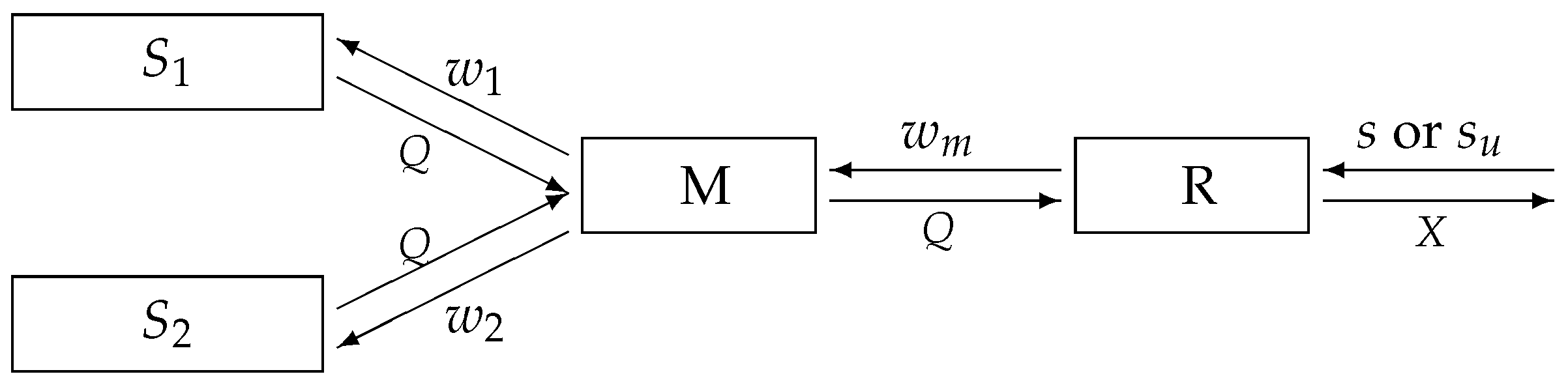
We model an assemble-to-order system involving two component suppliers, a single manufacturer and a single retailer under a single period. Before the beginning of the sales cycle (the primary inventory of the system is zero), the retailer works out
Q units of ordering quantity according to the forecast of the market demands and places an order with the manufacturer in advance. After ordering, the retailer cannot change the quantity. The manufacturer makes its corresponding decision based on the order from the retailer and respectively orders
Q units of necessary component
, which is offered by the supplier
. The final product
A is assembled out of components
and
. Each supplier only provides one kind of component, and the assembly ratio of component
to
is
. Supplier
decides the wholesale price
of component
. Once the necessary components are delivered, the manufacturer starts to assemble product
A immediately. After this is accomplished, it will be sent to the retailer at once. Suppose that the market demand of product
A a
X, and denote the CDF and PDF of
X by
and
, respectively. This form of assumption has been used in Christos and George [
30], Anastasios et al. [
31] and He and Zhao [
15]. The above supply chain can be modeled as in
Figure 1.
When the supply of component is suddenly disrupted with probability p before the start of the production period, the contingency plan replacing with the other component is urgently activated by the manufacturer. The manufacturer sends out Q units of the order of component to the spot market at once (the supply capacity is unlimited). The spot market decides the whole price of component . After the upgrade product is assembled, it will be delivered to the retailer. The manufacturer decides the wholesale price of product A or product .
After the sales cycle begins, on account of the shortage of product
A, customers can choose whether to purchase its upgrade product
according to their needs or preferences. That is, product
A can be replaced by its upgrade product
. We describe the substitution behavior of customers with probability
β in this paper. Obviously, the market demands of product
will be
. Relevant notations are shown in
Table 1.
We make the following assumptions to eliminate unrealistic cases.
Assumption 1. The system is risk-neutral; market information is symmetrical; and the decision-maker is entirely rational.
Assumption 2. The price of is not less than the price s of A, namely .
Assumption 3. .
Assumption 4. .
Assumption 5. , , , .
The assumptions above guarantee that the retailer, the manufacturer and the suppliers are willing to participate in the market. Similar forms of those assumptions have been widely used by many authors (e.g., He et al. [
12], He and Zhao [
15]), which are realistic.
4. The Performance of the Supply Chain under the Centralized Decision
In this section, we first obtain the expected profit function model of a three-echelon supply chain in terms of supply disruption and stochastic demand under centralized decision-making and then analyze the retailer’s optimal decision on the order quantity.
Based on the assumptions above, when the supply of supplier
is normal, the channel gross profit is:
where the first term is the total sales revenue for product
A, the second term is the manufacturing cost of the manufacturer and the third and fourth terms are the cost of supplier
producing component
. The last two terms are holding cost and shortage cost.
When the supply of component
is suddenly disrupted with probability
p, the channel gross profit is:
where the first term is the total sales revenue for product
, the second term is the manufacturing cost of the manufacturer, the third term is the running cost of buying component
of the spot market and the fourth term is the cost of supplier
producing component
. The fifth term is the lost cost of supplier
because of disruption. The last two terms are holding cost and shortage cost.
Hence, the gross profit function of the supply chain under centralized decision-making is given by the following expression:
or, equivalently,
Consequently, the expected profit function of the integrated supply chain can be expressed as:
Note that:
from the first order conditions of profit maximization, we obtain:
Denote the optimal order quantity of the supply chain under centralized decision-making by , and then, we have the following proposition.
Proposition 1. The expected profit function
is concave in
Q, and hence, there exists a unique
to maximize the integrated performance of the centralized supply chain, which satisfies Equation (
2).
Substituting Equation (
2) into Equation (
1), we obtain the maximal expected profit of the centralized supply chain as:
Proposition 1 indicates that the maximal profit function under centralized decision-making and the unique optimal order quantity exist. Hence, the main objective of the contract coordination in the decentralized supply chain is to make the order quantity of the retailer equal to .
5. Analysis on the Decentralized Supply Chain Based on Wholesale Price Contracts
This section considers each member’s profit in the decentralized supply chain under wholesale price contracts. We first develop the expected profit function model of the retailer and then use backward induction to obtain the maximal expected profit of each member. Lastly, we obtain that wholesale price contracts cannot coordinate the decentralized supply chain in terms of both supply disruption and stochastic demand.
5.1. The Retailer’s Expected Profit and Decision-Making
Based on the assumptions above, given the wholesale price set by the supplier and the manufacturer, respectively, the order quantity of the retailer and the profit function of the retailer are as follows.
When disruption occurs, the profit of the retailer is:
where the first term is the total sales revenue for product
, the second term is the purchase cost of
, i.e., the revenue of manufacturer, the third term is holding cost and the fourth term is the shortage cost.
When supply works normally, the profit of the retailer is:
where the first term is the total sales revenue for product
A, the second term is the purchase cost of product
A. The last two terms are the holding cost and shortage cost.
Hence, the expected profit function of the retailer can be expressed as:
Denote the optimal order quantity in the decentralized supply chain under wholesale price contracts by .
Proposition 2. The expected profit function
is concave in
Q, and the maximum,
, is uniquely solved by:
The proof of Proposition 2, as well as the proofs of other propositions are given in the
Appendix. Substituting Equation (
5) into Equation (
A1), we obtain the maximal expected profit of the retailer as:
5.2. The Expected Profit of the Supplier and Spot Market
Based on the assumptions and propositions above, we easily obtain that the maximal expected profit function of supplier
is:
The maximal expected profit of supplier
is:
and the maximal expected profit of spot market is:
5.3. The Expected Profit of Manufacturer
When the supply of supplier
is normal, the profit of the manufacturer is:
where the first term is the total revenue of the manufacturer, the second term is the manufacturing cost of the manufacturer and the third and fourth terms are the purchase cost of component
.
When the supply of component
from supplier
is disrupted with probability
p, the profit of the manufacturer is:
where the first term is the total revenue of the manufacturer, the second term is the manufacturing cost of the manufacturer, the third term is the cost of buying component
from the spot market and the fourth term is the cost of supplier
producing component
.
Consequently, the expected profit function of the manufacturer can be expressed as:
Set
; we then obtain the maximal expected profit of the manufacturer as:
Proposition 3. Under wholesale price contracts, the optimal order quantity in the decentralized supply chain, , is less than that of the supply chain based on centralized decision-making, , namely . Therefore, the wholesale price contracts cannot coordinate the decentralized supply chain.
Proposition 3 is similar to He and Zhao [
15], so we thus omit the proof.
6. Analysis on Decentralized Supply Chain Based on Buy-Back Contracts
In this section, we mainly pay attention to the decentralized supply chain under buy-back contracts. It can be seen from the above analysis that wholesale price contracts cannot coordinate the decentralized supply chain. Thus, we consider the other contract, buy-back contracts, in order to coordinate the supply chain.
Buy-back contracts, also called the return policy, mean that when the order quantity of the retailer is greater than the current demands at the end of the sales cycle, the manufacturer buys back unsold products from the retailer to encourage the retailer to order a larger quantity at the beginning of the next selling season.
6.1. The Retailer’s Expected Profit and Decision-Making
When supplier
supplies normally, the profit of the retailer is:
where
; the first term is the total sales revenue for product
A; the second term is the purchase cost of product
A; the third term is the return values from the manufacturer; and the fourth term is the shortage cost.
When supply disruption occurs, the profit of the retailer is:
where the first term is the total sales revenue for product
; the second term is the purchase cost of
, i.e., the revenue of manufacturer, the third term is the return values from the manufacturer and the fourth term is the shortage cost.
Therefore, the expected profit function of the retailer can be expressed as:
Note that:
from the first order conditions of profit maximization, we obtain:
Denote the optimal order quantity in the decentralized supply chain under buy-back contracts by ; we then have the following proposition.
Proposition 4. The expected profit function
is concave in
Q, and the optimal order quantity
is uniquely derived through solving Equation (
7).
Substituting Equation (
7) into Equation (
6), we obtain the maximal expected profit of the retailer as:
6.2. The Supplier’s and Spot Market’s Expected Profit
Apparently, the maximal expected profit function of supplier
is:
The maximal expected profit of supplier
is:
and the maximal expected profit of the spot market is:
6.3. The Manufacturer’s Expected Profit
When the supply of supplier
is normal, the profit of the manufacturer is:
where the first term is the total revenue of the manufacturer, the second term is the manufacturing cost of the manufacturer, the third and fourth terms are the purchase cost of component
, the fifth term is the buy-back cost and the last term is the holding cost.
When the supply of component
is disrupted with probability
p, the profit of the manufacturer is:
where the first term is the total revenue of the manufacturer, the second term is the manufacturing cost of the manufacturer, the third term is the cost of buying component
from the spot market, the fourth term is the cost of supplier
producing component
, the fifth term is the buy-back cost and the last term is the holding cost.
Consequently, the expected profit function of the manufacturer is given by:
Set
; we then obtain the maximal expected profit of the manufacturer as:
To make each member maximize their own profit while coordinating the supply chain, we can encourage the retailer to order the same amount as the centralized decision-making, namely,
. Combining Equations (
2) and (
7), we have:
or, equivalently,
From Equation (
8), we obtain:
we then have the following proposition.
Proposition 5. The decentralized supply chain can be coordinated by buy-back contracts, only if the buy-back parameter
b satisfies Equation (
9).
Proposition 5 presents a method to coordinate the decentralized supply chain channel through choosing a suitable buy-back parameter.
7. Numerical Examples
In this section, we present some numerical examples to gain further insights. We assume that the final demand faced by the retailer for the products A and is uniformly distributed over the interval . In our numerical study, the basic parameter values are given as: , , , , , , , , , , , , , . Demand has a mean of .
For the model under the centralized decision-making, the optimal order quantity of the retailer,
, and the optimal integrated performance,
, are given in
Table 2.
Table 2 reveals that an increase in the probability of the supply disruption damages the performance of the supply chain under centralized decision-making. As expected, the higher the market share,
β, is, the more integrated the performance,
, is.
Table 3 shows the optimal order quantity,
, each member’s maximal profit and the total profits,
, of the supply chain based on wholesale price contracts under decentralized decision-making. As the probability of disruption increases, both the order quantity of the retailer and the total profit of the supply chain will decrease. As expected, a higher
p reduces the expected profit of the manufacturer and supplier
, while positively influencing the retailer’s and spot-market’s profit.
Table 4 represents the optimal buy-back parameter,
, the optimal order quantity,
, the maximal profit of each member and the maximal channel profits,
, of the supply chain based on buy-back contracts under decentralized decision-making. As shown above, the higher the probability of disruption is, the less buy-back parameter
and the total profit of the supply chain are.
From
Table 2,
Table 3 and
Table 4, we find that the total profit of the supply chain under buy-back contracts can reach the integrated performance of the centralized decision-making through choosing a suitable buy-back parameter,
. Namely, buy-back contracts can efficiently coordinate the decentralized supply chain.
Denote the retailer’s maximal profit, the manufacturer’s, the spot market’s, and the maximal profit of the supplier
by R, M, SM and Si, respectively.
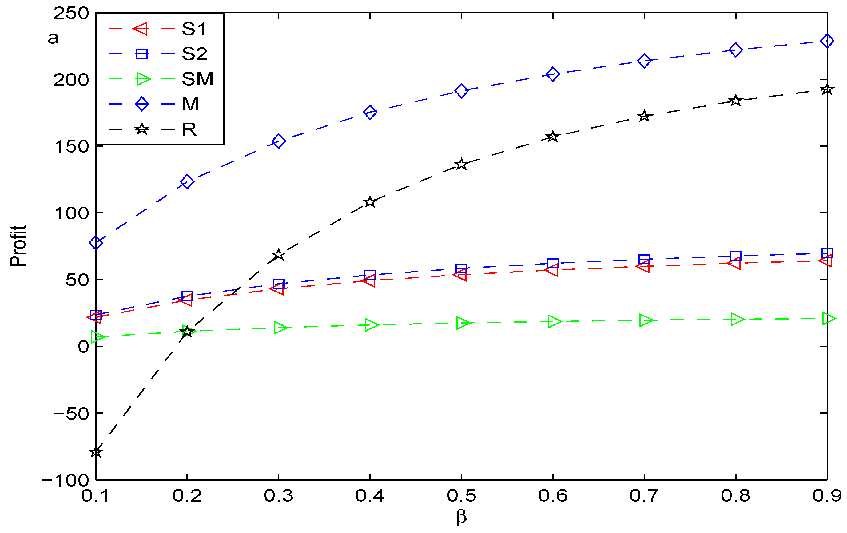
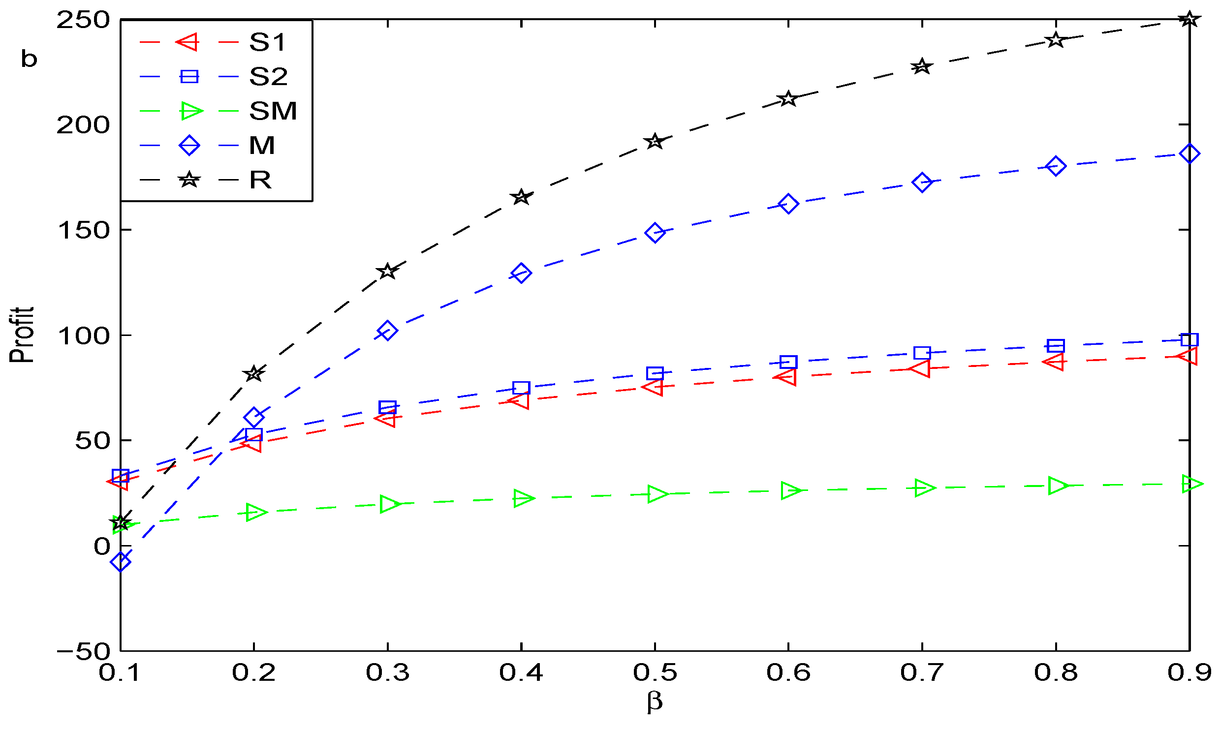
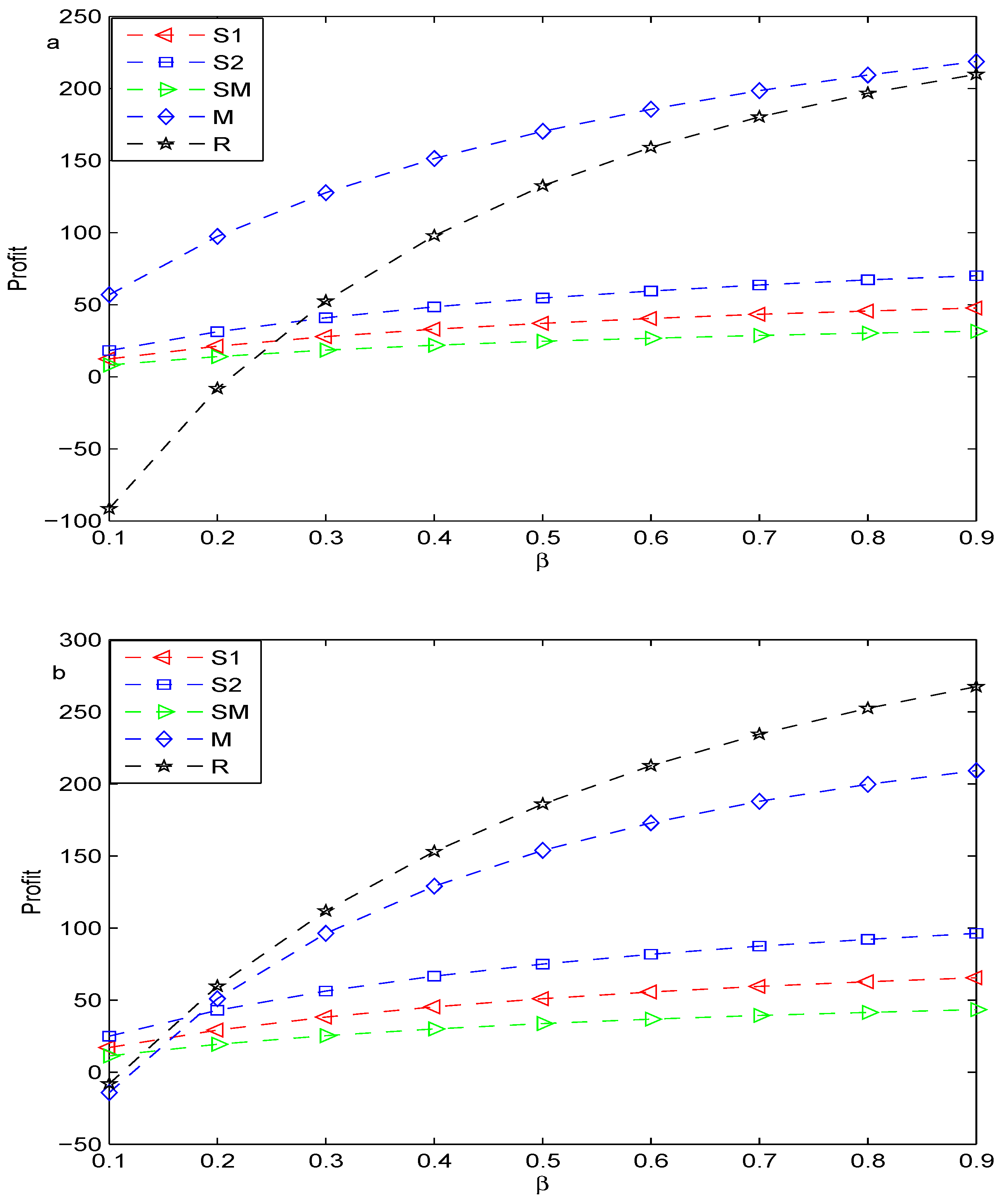
Figure 2,
Figure 3 and
Figure 4 compare the maximal profit of each member under wholesale price contracts with that under buy-back contracts in the decentralized supply chain when
, respectively. We find that coordination can enhance each member’s profit, except the manufacturer’s. As the probability of substituting product
for product
A increases, the maximal profit of each member increases in the sense of both wholesale price contracts and buy-back contracts.
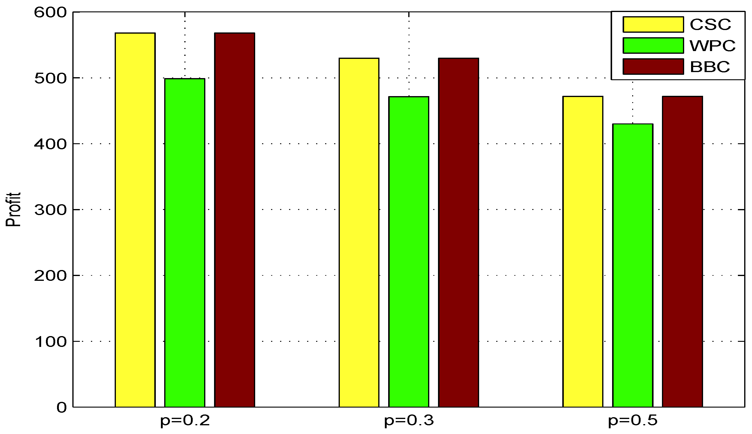
Denote the maximal total channel profits of the centralized supply chain, that of the decentralized system under wholesale price contracts and that of the decentralized system under buy-back contracts by CSC, WPC and BBC, respectively.
Figure 5 shows that the buy-back contracts can coordinate the decentralized supply chain more effectively than the wholesale price contracts when the supply of component
is disrupted, and the total channel profits under the decentralized decision can recover to the level of the centralized decision under the buy-back contracts.
8. Conclusions
This paper investigates the inventory decision of a retailer and the optimal contract in a multi-echelon supply chain in terms of both supply disruption and stochastic demand based on substitute products. We first obtained the optimal quantity of the supply chain under centralized decision-making. Then, we analyzed the corresponding profit function model under the decentralized decision in the case of wholesale price contracts and buy-back contracts, we found that the decentralized supply chain can be coordinated by buy-back contracts rather than by wholesale price contracts and then drew the conclusion that a properly-designed buy-back policy is able to efficiently coordinate the decentralized supply chain by comparing with the channel total profit under the centralized decision. In fact, we present a more effective method to make the channel total profit under the decentralized decision return to the level of that under centralized decision-making.
Our study is constrained by some assumptions and conditions, such as a single period, a single retailer, a single manufacturer, no stochastic supply, etc. Future research can be extended by relaxing or changing some assumptions and conditions made in this paper. For example,
- (1)
considering the optimal order quantity of the retailer under both stochastic demand and supply;
- (2)
giving a more detailed description and quantitative analysis for the influence of substitute products on the performance of the supply chain;
- (3)
considering a multi-period supply chain model based on both stochastic demand and supply.
All of the questions above may be worthwhile to derive theoretical results.


