A Novel Grey Wave Method for Predicting Total Chinese Trade Volume

Abstract

The total trade volume of a country is an important way of appraising its international trade situation. A prediction based on trade volume will help enterprises arrange production efficiently and promote the sustainability of the international trade. Because the total Chinese trade volume fluctuates over time, this paper proposes a Grey wave forecasting model with a Hodrick–Prescott filter (HP filter) to forecast it. This novel model first parses time series into long-term trend and short-term cycle. Second, the model uses a general GM (1,1) to predict the trend term and the Grey wave forecasting model to predict the cycle term. Empirical analysis shows that the improved Grey wave prediction method provides a much more accurate forecast than the basic Grey wave prediction method, achieving better prediction results than autoregressive moving average model (ARMA).

1. Introduction

With the integration of the global economy, international trade has developed rapidly and has become an indispensable source of economic growth. Fluctuations in total trade volume affect not only a country’s economic growth but also its international trade situation. An increasing number of countries earn large revenues from international trade. Total trade volume significantly influences countries’ economies and is an important indicator of a country’s international trade situation. A trade volume forecast helps enterprises to schedule their production efficiently and promote sustainable international trade. For these reasons, it is important for company managers to forecast total trade amounts for relevant government departments and business investors. A trade volume forecast is subject to complicated factors, and because of its complex and irregular patterns, it still has not been explained fully in the academic literature. Consequently, the demand for the accurate modeling and forecasting of trade volume has increased. At present, methods of forecasting total import and export trade are divided into three categories: the linear prediction method, the nonlinear prediction method, and a combination forecasting method. While linear prediction is simple and intuitive, and its parameters have strong economic significance, it has difficulty in fitting complex data [1,2]. The advantage of nonlinear prediction is that it can fit a complicated nonlinear system, so nonlinear predictions have better fitting precision than linear predictions for nonlinear import and export trade volumes [3,4,5]. The combination forecasting method addresses these shortcomings by integrating multiple single-prediction models, including linear and nonlinear prediction models, using advantages of both models to obtain better predictions results [6,7,8]. In this paper, the Grey wave prediction method with an HP filter combines linear and nonlinear predictions, thereby improving prediction accuracy.

Grey system theory [9,10], proposed by Professor Deng, is based on various forms of uncertainty information theory and methods, characterized by small data amounts that can disregard data distribution. The theory is applicable in many fields [11,12,13].

The Grey prediction model is one of the most active and widely used Grey system models. Some data processing programs can scientifically and quantitatively predict the future of a system. Grey prediction models have numerous applications. For instance, Chirwa and Mao, using U.S. and UK data, applied a GM (1,1) model to estimate the risk of car accidents [14]; Cempel used a Grey prediction model to monitor the state of mechanical vibration [15]; Grey system models were also used to analyze and predict hydraulic processes at the Karst watershed [16,17]; Wang adopted a Grey neural network method for the Chinese civil aviation operation’s nonlinear, on-line prediction model [18]; and Li et al. used a Grey system model to predict spacecraft failure [19].

Nearly all previous studies used the GM (1,1) or GM (1,N) model to derive predictions [20,21,22] for monotonic time series. While these studies showed very effective results with high prediction accuracy [23], they are not suitable for cyclical fluctuations and a wide range of data series. Many researchers propose that GM (1,N) models be modified on the basis of the characteristics of data series. For a series of fluctuating data, Feng proposed the GM (1,1, sinω) model [24], and Qian and Dang proposed an oscillation series in the GM (1,1) model. However, the application of both models is very limited [25]. Only Guo et al. used GM (1,1, sinω) to predict epidemiological trends of hemorrhagic fever and renal syndrome in Shenyang [26]. The GM (1,1) model, which is based on an oscillation series, is only proven by a numerical example. Both models of mathematical theory are very complex, and few practitioners can master them. In addition, these two models only apply to stable fluctuations in data series; in other words, they are not suitable for time series with growth trends.

Grey wave predictions based on data series predictions are one of the most important research topics in Grey system prediction research. Grey wave prediction models not only have the advantage of a Grey system prediction model but also that of forecasting short-term fluctuations of time series based on limited data [27,28]. These models do not consider the distribution and stability of a time series. In fact, the Grey wave prediction model accurately predicts data series with large fluctuations, such as that of Chen et al., who analyzed an economic cycle using a Grey wave forecasting model and proposed Grey wave prediction in the economic cycle [29]. However, there is little research regarding Grey wave prediction models for time series forecasting, let alone an improved model for Grey wave forecasting, when compared with the explosive growth of studies on GM (1,1) or GM (1,N) [22,30,31,32,33]. A pioneer in Grey wave prediction is by Wan et al., who advanced a basic Grey wave prediction model beyond data series with a regular fluctuation range based on a data series and trough selection contours [34]. However, this method is inefficient because all crests and valleys are found to carry heavy workloads. Chen proposes a non-equidistant Grey wave prediction model that begins with selecting qualified contour lines and using a GM (1,1) model. This method, however, is only applicable to time series that do not have significant trends [35]. A few international studies exist regarding oscillation series with obvious trend characteristics. Chen proposed a Grey wave prediction method based on general contours. This method uses the least squares method to select contours, which can make up for shortcomings in a Grey wave prediction model by applying ascending and descending trend data [36]. Based on the above research, this paper proposes a Grey wave prediction model with an HP filter that aims to reduce the interference of long-term trend items, using wave prediction by trend decomposition. After applying an improved Grey wave prediction model to China’s total trade volume forecast, this paper concludes that a Grey wave prediction with an HP filter can improve the accuracy of non-equidistant Grey wave predictions.

2. A Grey Wave Prediction Model with an HP Filter

Grey wave prediction is a graphical prediction method that uses information from a time series data graph to predict future series. It focuses on irregular, developing trends of data series, and it is applicable to data series with frequent and irregular fluctuations. Contours are selected and identified to pick up graphical information. The principle is to obtain coordinate information regarding the intersection of the contour lines and the data graph.

Finally, GM (1,1) is used to forecast and model intersections. To improve the adaptability of a Grey wave forecasting model in a fluctuating data series with increasing or decreasing trends, a Grey wave forecasting model with an HP filter is proposed in this research.

2.1. The HP Filter

Proposed by Hodrick and Prescott (1980), an HP filter [37,38,39] method is adopted to eliminate the long-term tendency of a time series in economics. This method is widely used in the field of macroeconomics. An HP-filtering method is a time series decomposition method in state space. The HP-filtering method assumes that macroeconomic data is composed of a long-term tendency and a short-term circulation. Trend decomposition is the first step of a Grey wave prediction model with an HP filter. A traditional Grey wave prediction model is based on original data; hence, subject to trend term interference, it is easy to create a prediction effect of the model.

Given $n$ observations on a variable $s_i$, $t_i$ is the trend component as a smooth series that does not differ too much from the observed $s_i$. The tendency of total trade volume can be decomposed through optimization:

$$\min \left\{{\displaystyle \sum _{t=1}^n{(s_i-t_i)}^2+\lambda {\displaystyle \sum _{t=2}^{n-1}{\left[(t_{i+1}-t_i)-(t_i-t_{i-1})\right]}^2}}\right\}$$

(1)

As we mentioned before, for minimization, we use $\lambda$ to adjust any changes in the long-term trend. When $\lambda =0$, which means that the trends satisfy the minimization problem (in this connection, with increasing $\lambda$), we estimate a smoother tendency, moving toward infinity, with a quasi-linear, long-term trend.

2.2. Predictions of Tendency

The main task of this step is to find a series of trends after HP filtering. We apply a GM (1,1) model to fit and predict the trend series.

Definition: Assume that $T^{(0)}$ is an original series $T^{(0)}=(t^0(1),t^0(2),\cdots t^0(n)),n\ge 1$. Let $T^{(0)}$ be the raw data series, generating the first-order accumulated generating operation (AGO) series $T^{(1)}$, where:

$$t^{(1)}(k)={\displaystyle \sum _{i=1}^k{t}^{(0)}(i)},t^0(i)\ge 0,k=1,2,\cdots ,n$$

(2)

The first-order differential equation of the GM (1,1) model is obtained as follows:

$$\frac{d{t}^{(1)}(x)}{dx}+a{t}^{(1)}(x)=u$$

(3)

By using the least squares method, parameters $a$ and $u$ can be obtained as follows:

$$\begin{array}{l}\widehat{a}=\left(\begin{array}{c}a\\ u\end{array}\right)={\left(B^{T}B\right)}^{-1}{B}^T{y}_n\\ \end{array}$$

$Z^{\left(1\right)}\left(k\right)$ is the sequence mean generated based on consecutive neighbors of $X^{\left(1\right)}\left(k\right)$.

$$z^{(1)}(k)=0.5x^{(1)}(k)+0.5x^{(1)}(k-1)$$

Furthermore, an accumulated matrix B and vector $y_n$ are given by the following:

$$B=\left[\begin{array}{c}\begin{array}{cc}-z^{(1)}(2)& 1\\ -z^{(1)}(3)& 1\end{array}\\ \begin{array}{cc}⋮& ⋮\\ -z^{(1)}(n)& 1\end{array}\end{array}\right],y_n={(t^{(0)}(2),t^{(0)}(3),\cdots ,t^{(0)}(n))}^T$$

The discrete form of the solution for the GM (1,1) model is given below.

$${\widehat{t}}^{(1)}(k+1)=(t^0(1)-\frac{u}{a})e^{-ak}+\frac{u}{a},k=1,2\cdots ,n$$

(4)

The recovered data ${\widehat{t}}^{(0)}(k+1)$ can be retrieved from the following equation:

$$\{\begin{array}{c}{\widehat{t}}^{(0)}(k+1)={\widehat{t}}^{(1)}(k+1)-{\widehat{t}}^{(1)}(k)\\ {\widehat{t}}^{(0)}(1)={\widehat{t}}^{(1)}(1)\end{array}$$

2.3. Prediction of Circulation

The purpose of this step is to obtain a series of circulation after HP filtering. We use a Grey wave prediction model to fit and predict the cycle series.

2.3.1. Choosing Contour Lines

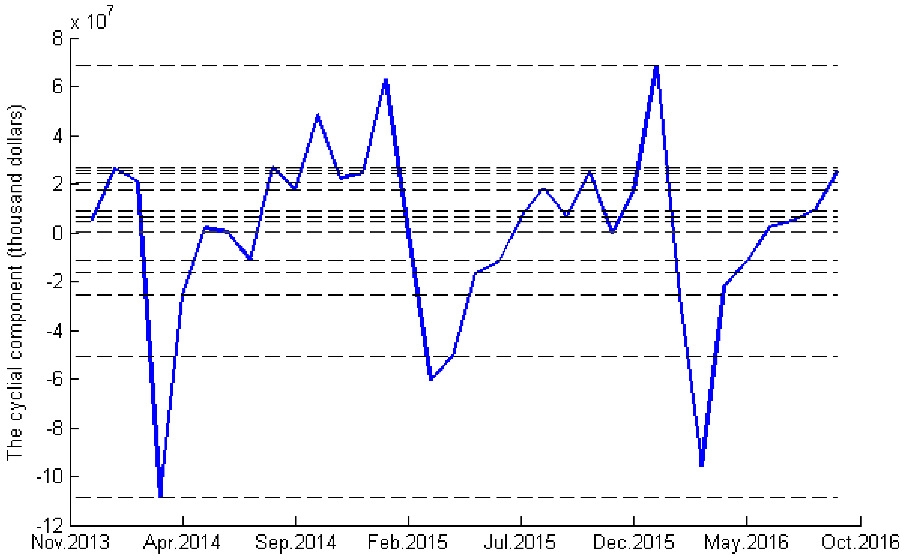
Original Grey wave prediction models utilize horizontal contour lines, which only achieve preferable prediction results when using data series with steady, periodic fluctuations. However, because economic data fluctuates with upward and downward tendencies, an original Grey wave forecasting model is no longer suitable for this type of data series. Therefore, we choose to use the quantile of time series as a contour line to seize graphical information correctly proposed by Chen (2016) [36] (shown in Figure 1).

Definition 1.

(unequal-interval contour lines):

Let the original series be $X=(x(1),x(2),\cdots ,x(n))$, and sort the series in ascending order to get $X^a=(x^a(1),x^a(2),\cdots ,x^a(n))$.

Let ${\xi }_0=x^a(1)$, ${\xi }_S=x^a(n)$, and let $({\xi }_1,{\xi }_2,\cdots ,{\xi }_{s-1})$ be the $s$-quantile of the data $X^a$, where the i ths-quantile is:

$${\zeta }_i=\{\begin{array}{cc}{x}^d\lceil I_p\rceil \hfill & \hspace{1em}\hspace{1em}{I}_p \mathrm{is} \mathrm{not} \mathrm{a} \mathrm{integer}\\ [x^d(I_p)+x^d(I_p+1)]/2& \hspace{1em}\hspace{1em}\hspace{1em}\hspace{1em}{I}_p \mathrm{is} \mathrm{a} \mathrm{integer}\end{array}$$

where $I_p=n\times (i/s)$, the $s+1$ horizontal lines decided by $({\xi }_0,{\xi }_1,{\xi }_2,\cdots ,{\xi }_{s-1},{\xi }_s)$ are unequal-interval contour lines.

2.3.2. Identifying Contour Time Series

The contour time series should be determined according to the quantile of short-term cycle time series. Each element of a contour time series is the abscissa of the intersection point between contour lines and a short-term cyclic time series graph.

Definition 2.

(contour time series):

Let the cyclic time series be $C=(c(1),c(2),\cdots ,c(n))$, with contour line ${\xi }_i$ intersecting with the original time series, and let $C_{{\xi }_i}=(P_1,P_2,\cdots ,P_m)$ be the set of intersection points. $P_j$ is located on the $t_j$th broken line, and the coordinates of $P_j$ are as follows:

$$(c_j+\frac{{\xi }_j-c(t_j)}{c(t_j+1)-c(t_j)},{\xi }_j)$$

and let:

$$q(j)=t_j+\frac{{\xi }_j-c(t_j)}{c(t_j+1)-c(t_j)},j=1,2,\cdots ,m$$

(5)

where by $Q^{(0)}=(q(1),q(2),q(3),\cdots ,q(m)),i=0,1,2,\cdots ,s$ is the contour time series of contour line $\xi$.

2.3.3. Filtrating Contour Time Series

The basic Grey wave prediction method is based on a contour time series of four or more values. However, when the time series fluctuates violently with a long-term tendency component (as shown in Figure 1), the different number of intersection points for different contour lines is obvious. Therefore, the traditional method, based on four or more values, is not appropriate, and the contour time series needs to be filtered to perform the GM (1,1) prediction process.

This paper uses autocorrelation of time series to select the contour lines, which means that future series observations will be affected by current or late observations. Therefore, when the last value of the contour time series is close to the first forecasted observation, we choose it as the qualified contour time series. The rest are defined as unqualified contour time series.

Definition 3.

(qualified and unqualified contour time series):

Let $t_1^f$ be the first predicted observation and $Q_i^{(0)}=(q_i(1),q_i(2),\cdots ,q_i(m_i))$. If $t_1^f-q_i(m_i)$ is less than or equal to the threshold $D$, $Q_i^{(0)}$ is the qualified contour time series. If $t_1^f-q_i(m_i)$ is larger than the threshold $D$, $Q_i^{(0)}$ is the unqualified contour time series.

2.3.4. Establishing GM (1,1) Models

For the final step, we use GM (1,1) models based on qualified contour time series for both in-sample fitting and out-of-sample forecasting, and we use GM (1,1) models based on unqualified contour time series only for in-sample fitting.

Proposition 1 establishes GM (1,1) based on $Q_i^0=(q_i(1),q_i(2),\cdots ,q_i(m_i))$ to obtain forecasting values ${\widehat{q}}_i(m_i+1),{\widehat{q}}_i(m_i+2),\cdots \cdots ,{\widehat{q}}_i(m_i+k_i)$.

Sort all the values in contour time series $Q_0^{(0)},Q_1^{(0)},Q_2^{(0)}\cdots \cdots ,Q_s^{(0)}$ in ascending order, and delete invalid elements. The forecasting series is as follows:

$$\begin{array}{l}\widehat{q}(1)<\widehat{q}(2)<\cdots <\widehat{q}(n_i)\\ n_i={\displaystyle \sum _{i=1}^s(m_i+m_k)}\end{array}$$

In which $n_i\le {\displaystyle \sum _{i=1}^s(m_i+m_k)}$. If $\widehat{q}(k)$ is on contour line ${\xi }_{\widehat{q}(k)}$, the generated wave through in-sample modeling and out-of sample prediction is:

$$X={\widehat{X}}^{(0)}=\left\{{\xi }_{\widehat{q}(k)}+\frac{t-\widehat{q}(k)}{\widehat{q}(k+1)-\widehat{q}(k)}\left[{\xi }_{\widehat{q}(k+1)}-{\xi }_{\widehat{q}(k)}\right]|k=1,2\cdots ,n_s\right\}$$

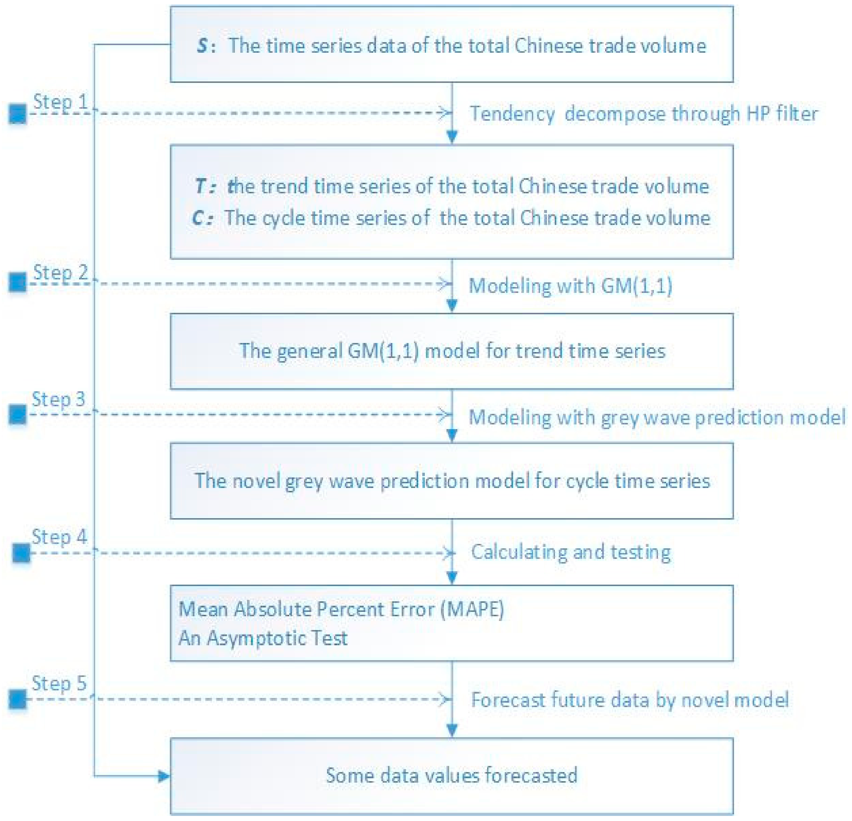
The novel Grey wave predicting procedure of total Chinese trade volume mentioned above is shown in Figure 2.

3. Empirical Studies

3.1. Data

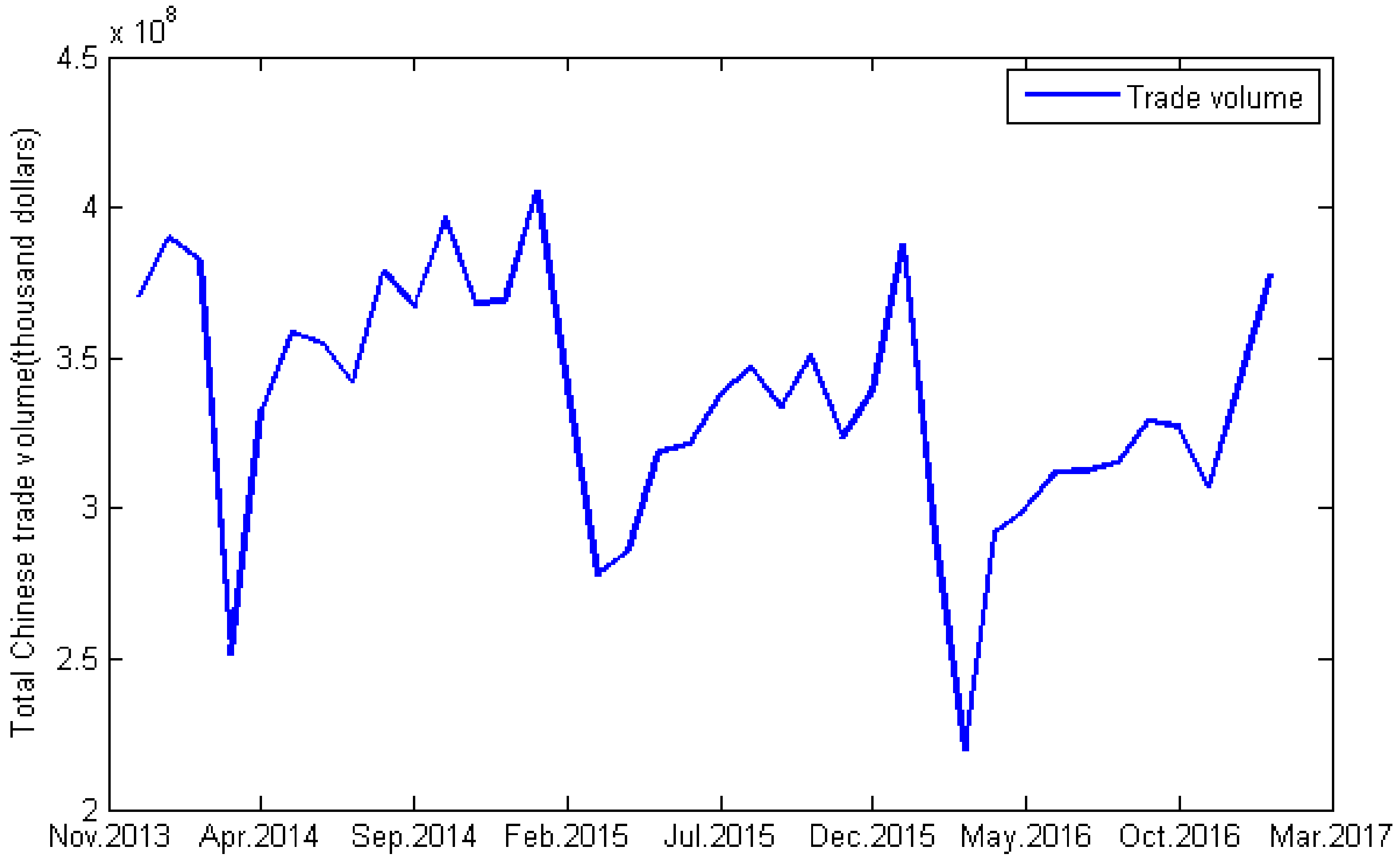
In this study, we use monthly trade data of the total Chinese import and export trade volume, a valid estimation of international trade. The data are prepared and obtained from the National Bureau of Statistics of the People’s Republic of China. Datasets span from November 2013 to December 2016. Figure 3 indicates the frequent and irregular fluctuations in total trade volume.

3.2. The Forecasting Process

This study divides the datasets into two parts: an in-sample data form November 2013 to August 2016 (34 observations) and an out-of-sample data from September 2016 to December 2016 (four observations). In-sample data, which are applied to select contour lines, determine contour time series. Out-of-sample data appraise predictive performance. We expect a four-step prediction process.

Table 1. Autocorrelation analysis of monthly trade volume.

	Lag	1	2	3	4	5	6	7	8	9	10
Trade Volume	AC	0.9690	0.9500	0.9470	0.9390	0.9230	0.9140	0.9050	0.9040	0.8930	0.8810
	Prob.	0.0000	0.0000	0.0000	0.0000	0.0000	0.0000	0.0000	0.0000	0.0000	0.0000

lists the autocorrelation coefficients from 1 to 10 lags. It indicates that the total trade volume incorporates autocorrelation; hence, we can use Definition 3 to classify contour time series.

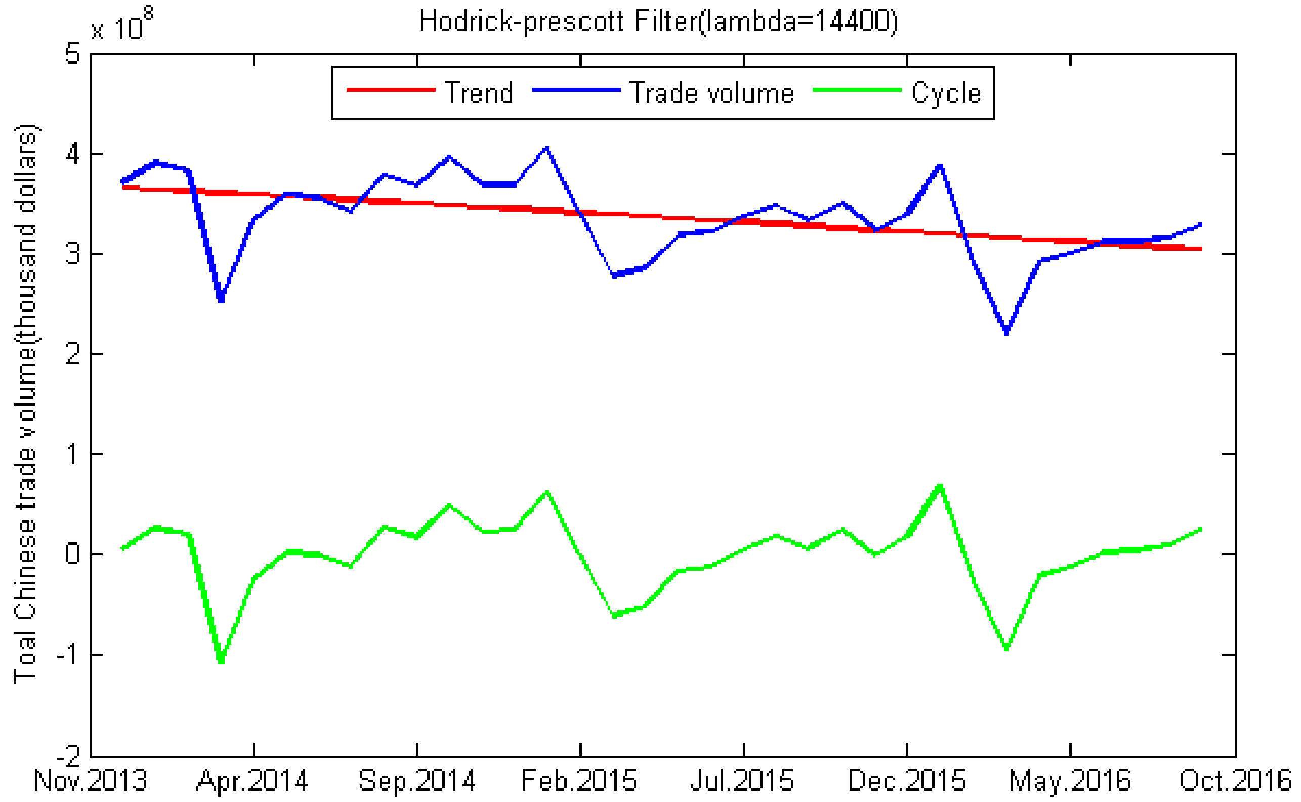
This paper uses a Hodrick–Prescott filter to further decompose long-term trend items and short-term cycle items. According to an ordinary decomposition of the monthly time series, λ was set to 14,400. The result of Hodrick–Prescott filter is shown in Figure 4.

We divide the prediction process into two parts. The first part establishes the GM (1,1) model to predict long-term tendencies, and the second part predicts short-term cyclic time series.

3.2.1. Tendency-Component Prediction

The first part of the Grey forecasting process established the GM (1,1) model to forecast long-term tendency series.

By using the least squares method, matrix $B$ and vector $y_n$ are as follows:

$$B=\left[\begin{array}{cc}\begin{array}{c}-z^{(1)}(2)\\ -z^{(1)}(3)\\ ⋮\\ -z^{(1)}(n)\end{array}& \begin{array}{c}1\\ 1\\ ⋮\\ 1\end{array}\end{array}\right]=\left[\begin{array}{cc}\begin{array}{c}-546795480.10\\ -909332142.15\\ ⋮\\ -11249319045.30\end{array}& \begin{array}{c}1\\ 1\\ ⋮\\ 1\end{array}\end{array}\right],y_n=\left[363390977.60,361682346.50,\cdots ,303987520.00\right]$$

$$\widehat{a}=\left(\begin{array}{c}a\\ u\end{array}\right)={\left(B^{T}B\right)}^{-1}{B}^T{y}_n=\left(\begin{array}{c}0.00559\\ -368247792.22\end{array}\right)$$

According to Equation (3), the first-order differential equation of the GM (1,1) model is as follows:

$$\frac{d{t}^{(1)}(x)}{dx}+0.00559t^{(1)}(x)=-368247792.22$$

The solution of the GM (1,1) model is as given below.

$${\widehat{t}}^{(1)}(k+1)=\left[t^{(0)}(1)-\frac{u}{a}\right]e^{-ak}+\frac{u}{a}=-65429472272.57e^{-0.00559k}-65794572263.88$$

3.2.2. Cyclical Component Predictions

The second part of the forecasting process involves predicting the short-term cyclic time series. Fourteen contour lines are shown, as follows:

$$Q_1^{(0)}=(4)$$

$$Q_2^{(0)}=(26)$$

$$Q_3^{(0)}=(11.00,13.62,14.23,25.60,26.21)$$

$$Q_4^{(0)}=(14.00,25.89,26.06)$$

$$Q_5^{(0)}=(3.63,4.58,16.00,27.50,28.47)$$

$$Q_6^{(0)}=(3.90,4.16,28.00)$$

$$Q_7^{(0)}=(3.36,9.91,13.22,17.64,23.54,31.41)$$

$$Q_8^{(0)}=(3.25,8.44,12.39,18.17,26.66)$$

$$Q_9^{(0)}=(3.16,5.92,7.02,8.29,15.00,19.64,24.00,24.01)$$

$$Q_{10}^{(0)}=(3.12,12.94,15.10,17.63,20.58,24.02,28.04,32.73)$$

$$Q_{11}^{(0)}=(1.04,3.11,8.46,14.90,20.00,21.99,22.00,23.75)$$

$$Q_{12}^{(0)}=(1.60,3.02,8.76,9.93,10.02,14.71,21.00,22.61,23.29)$$

$$Q_{13}^{(0)}=(1.91,6.68,7.75,8.99,10.43,12.10,14.04,16.29,18.89,21.92,25.43,29.50,34.23)$$

$$Q_{14}^{(0)}=(9.00 ,8.96,11.14,13.85,17.21,21.39,26.58,33.03)$$

Since the serial number of the first forecasting observation is 38, and the data show autocorrelation according to Table 1, this paper chooses $Q_{10}^{(0)}$, $Q_{11}^{(0)}$, $Q_{12}^{(0)}$, $Q_{13}^{(0)}$, and $Q_{14}^{(0)}$ as qualified contour time series. Other counter series are just for in-sample fitting purposes.

The final step involves GM (1,1) to predict the contour time series. In this section, we only give the time-modeling series of a qualified contour time series $Q_{10}^{(0)}$, $Q_{11}^{(0)}$, $Q_{12}^{(0)}$, $Q_{13}^{(0)}$, and $Q_{14}^{(0)}$. The modeling process of the remaining contour time series is the same.

$${\widehat{q}}_{10}^{(1)}(k+1)=\left[q_{10}^{(0)}(1)-\frac{u}{a}\right]e^{-ak}+\frac{u}{a}=77.26e^{0.16k}-74.14$$

$${\widehat{q}}_{11}^{(1)}(k+1)=\left[q_{11}^{(0)}(1)-\frac{u}{a}\right]e^{-ak}+\frac{u}{a}=81.76e^{-1.04k}-80.72$$

$${\widehat{q}}_{12}^{(1)}(k+1)=\left[q_{12}^{(0)}(1)-\frac{u}{a}\right]e^{-ak}+\frac{u}{a}=52.77e^{0.15k}-51.17$$

$${\widehat{q}}_{13}^{(1)}(k+1)=\left[q_{13}^{(0)}(1)-\frac{u}{a}\right]e^{-ak}+\frac{u}{a}=41.71e^{0.15k}-39.80$$

$${\widehat{q}}_{14}^{(1)}(k+1)=\left[q_{14}^{(0)}(1)-\frac{u}{a}\right]e^{-ak}+\frac{u}{a}=36.91e^{0.22k}-27.91$$

Let ${\widehat{q}}_i(k+1)={\widehat{q}}_i(k+1)-{\widehat{q}}_i(k)$; thus, the forecasting value of the contour time series is as follows:

$${\widehat{Q}}_{10}^{(0)}=({\widehat{q}}_{10}(9),{\widehat{q}}_{10}(10))=(44.81,57.04)$$

$${\widehat{Q}}_{11}^{(0)}=({\widehat{q}}_{11}(12),{\widehat{q}}_{11}(13))=(37.99,40.89)$$

$${\widehat{Q}}_{12}^{(0)}=({\widehat{q}}_{12}(13),{\widehat{q}}_{12}(14))=(40.58,45.43)$$

$${\widehat{Q}}_{13}^{(0)}=({\widehat{q}}_{13}(14),{\widehat{q}}_{13}(15))=(40.13,44.93)$$

$${\widehat{Q}}_{14}^{(0)}=({\widehat{q}}_{14}(8),{\widehat{q}}_{14}(9))=(33.35,41.86)$$

3.3. Forecasting Results

To better reflect the superiority of a novel Grey predicting method, this paper chooses the improved basic method (using unequal-interval contour lines) and the most commonly used model in time series analysis ARMA (1,3) to forecast China’s total monthly trade volume.

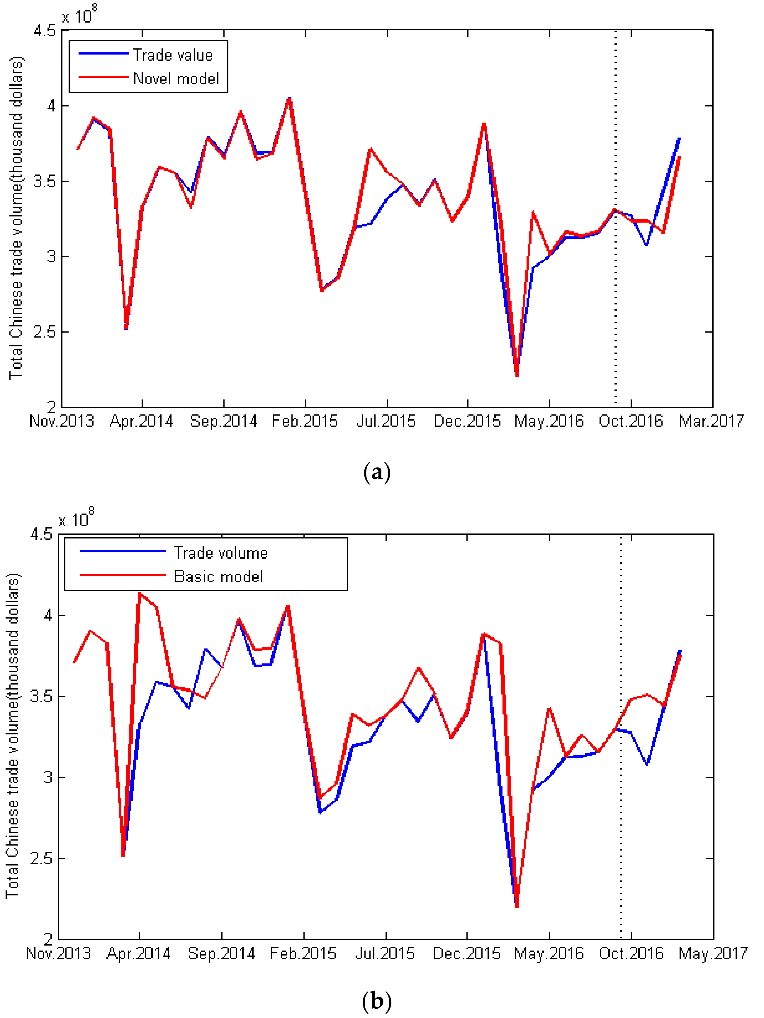
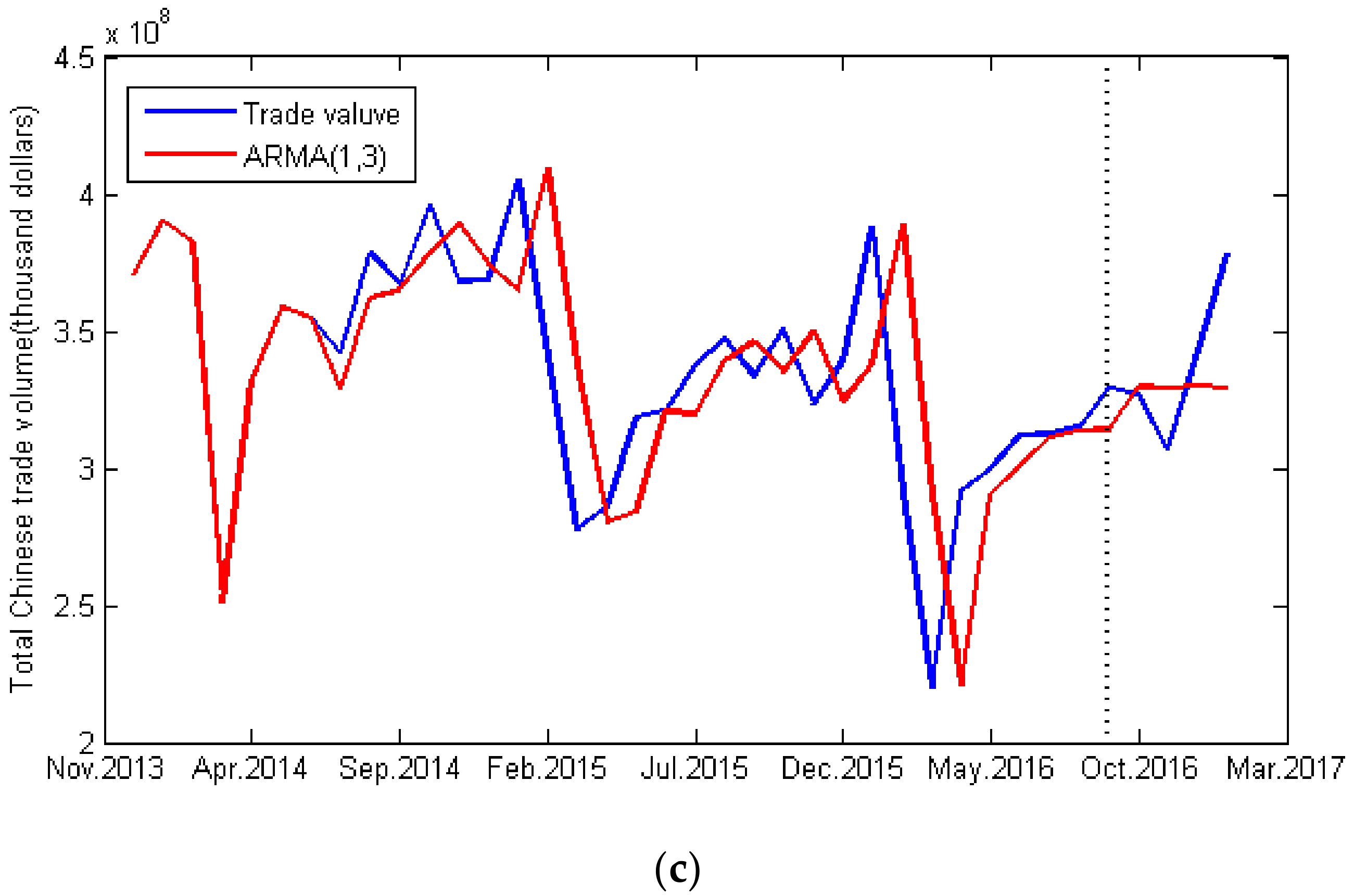
We use the Mean Absolute Percentage Error (MAPE) to evaluate the prediction accuracy of the model.

Table 2. Prediction accuracy comparison of different methods.

Method	In-Sample Data	Out-of-Sample Data
	MAPE	MAPE
Basic method	0.0471	0.0872
Novel method	0.0466	0.0444
ARMA (1,3)	0.0673	0.0618

suggests that the predictive effect of an improved Grey wave prediction method is superior to the basic method, in both modeling and predicting. Although the performance of ARMA (1,3) is better than those of the basic methods for out-of-sample forecasting, the novel Grey wave prediction method is significantly superior to the above mentioned two models, whether using in-sample data-fitting or out-of-sample predictions. Figure 5 compares the forecasting results. In a four-step prediction, ARMA (1,3) tracks the movement of the existing trade volume closely, which affects the accuracy of prediction, whereas the improved method considers possible fluctuations.

3.4. An Asymptotic Test

The asymptotic test is a statistical method used to test the equality of the forecast accuracy [40]. It uses the null hypothesis of equal forecast accuracy for two forecast methods to test the accuracy of the prediction models. The asymptotic test does not assume the distribution of the loss, and there is no limitation to the loss function. Therefore, the asymptotic test is more practical to compare the predictive accuracy of the models.

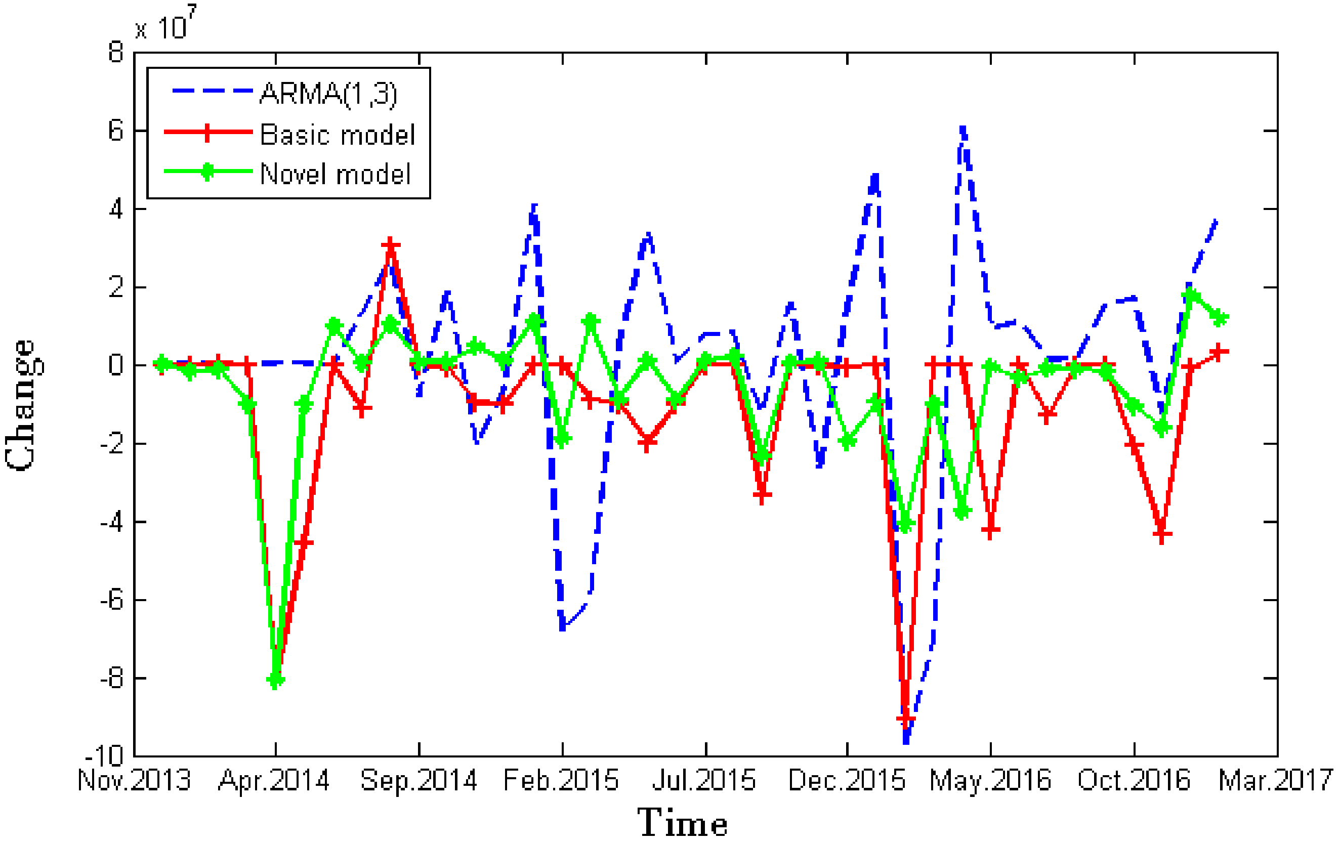
We assess two forecasts, the basic grey wave forecast and the forecast implicit in the grey wave prediction model with HP filter (the difference between the basic model and the novel model). As ARMA forecast have been widely used in time series forecast, we chose ARMA model as the “no change” forecast.

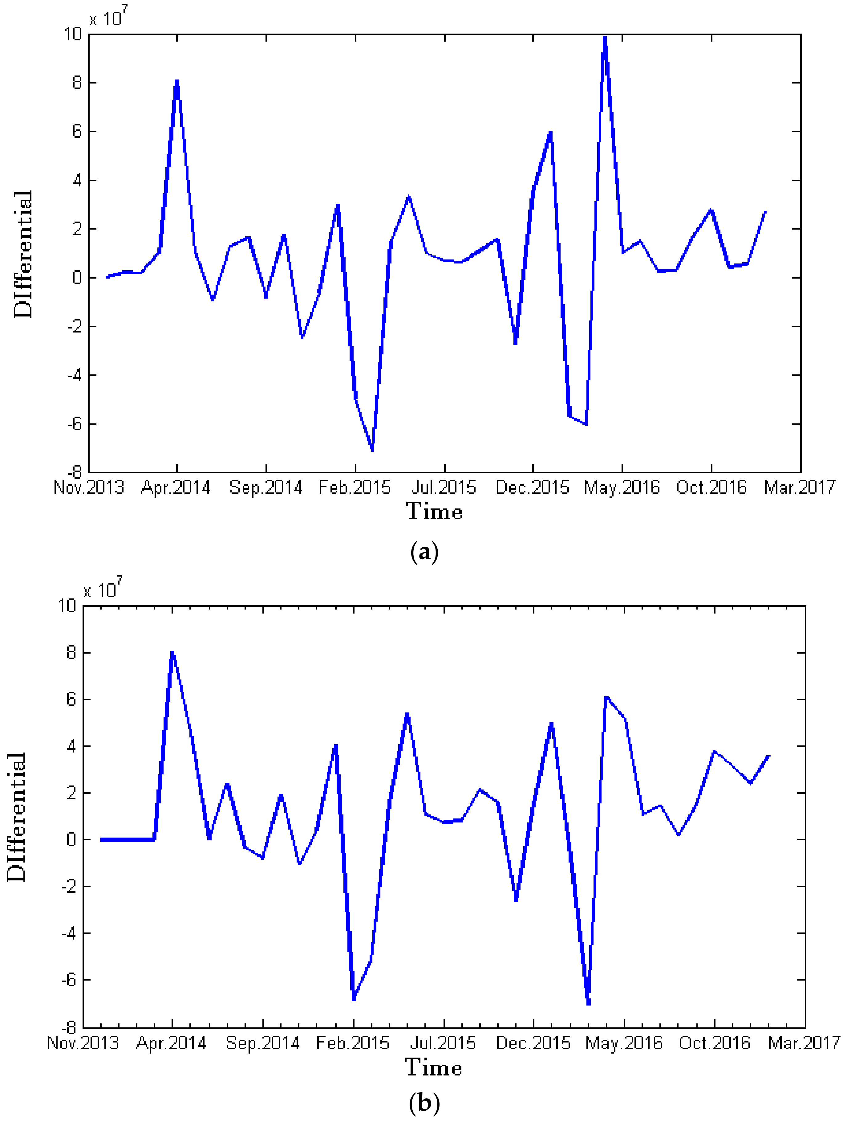
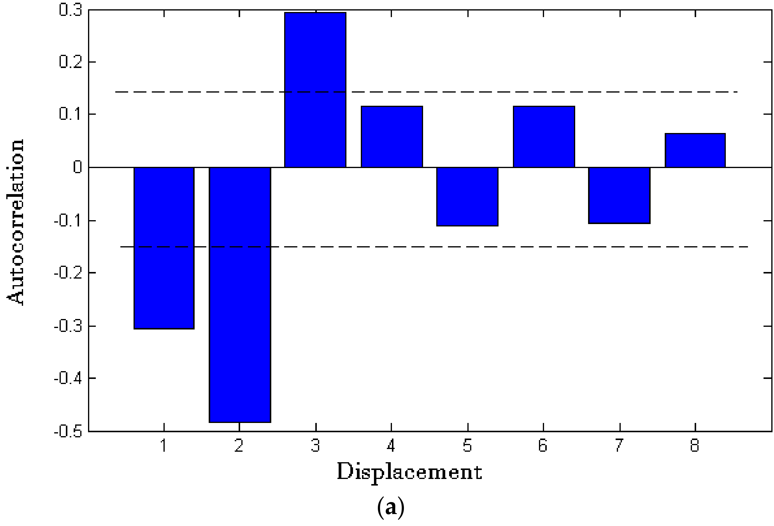
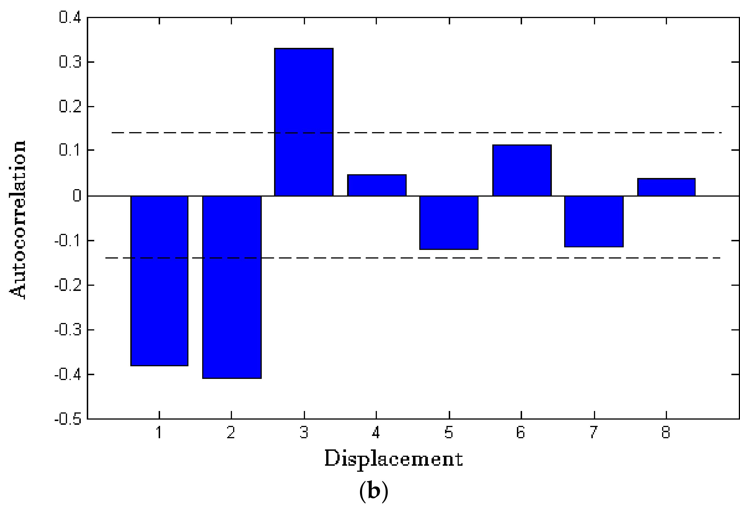
The actual and predicted changes are shown in Figure 6. We shall assess the forecasts’ accuracy under absolute error loss. The loss differential series is shown in Figure 7, in which no obvious non-stationarities are visually apparently. Approximate stationarity is also supported by the sample autocorrelation function of the loss differential, shown in Figure 8, which decays quickly.

Because the forecasts are four-step-ahead, according to the condition of the asymptotic test, the forecast allows least three-dependent forecast error. This intuition is confirmed by the sample autocorrelation function of the loss differential, in which sizable and significant sample autocorrelation appear at lags 1, 2 and 3 and nowhere else.

We then proceed to test the null of equal expected loss. F, MGN, and MR are inapplicable because one or more of their maintained assumptions are explicitly violated. The statistic for testing the null hypotheses of equal forecast accuracy is

$$S_1=\frac{\overline{d}}{\sqrt{\frac{2\pi {\widehat{f}}_d(0)}{T}}}$$

where ${\widehat{f}}_d(0)$ is a consistent estimate of $f_d(0)$.

By taking a weight sum of the available sample autocovariances,

$$2\pi {\widehat{f}}_d(0)={\displaystyle \sum _{\tau =-(T-1)}^{(T-1)}1(\frac{\tau }{S(T)})}\widehat{\gamma }(\tau )$$

where:

$$\widehat{\gamma }(\tau )=\frac{1}{T}{\displaystyle \sum _{t=\left|\tau \right|+1}^T(d_t-\overline{d})(d_{t-\left|\tau \right|}-\overline{d})}$$

$S\left(T\right)$ is the truncation lag$1\left(\tau /S\left(T\right)\right)$ is the lag window, defined as follows:

$$\begin{array}{c}\begin{array}{cc}1(\frac{\tau }{S(T)})\widehat{\gamma }(\tau )=1& for\left|\frac{\tau }{S(T)}\right|\le 1\end{array}\\ \begin{array}{cc}1(\frac{\tau }{S(T)})\widehat{\gamma }(\tau )=0& \begin{array}{cc}otherwise& \end{array}\end{array}\end{array}$$

We therefore focus on test statistic $S_1$ setting the truncation lag at 3 in light of the preceding discussion. We obtain $S_1$ of the novel model is negative 1.2391, implying a p value of 0.2178. Thus, for the sample at hand, we do not reject at conventional levels the hypothesis of equal expected absolute error. Moreover, we can also obtain $S_1$ of the basic model is negative 1.7925 with a p value of 0.1936, the result is the same as the novel model, which means that both the basic Grey wave forecast and the novel Grey wave forecast are not a statistically significantly worse predictor of the future total trade volume than is the ARMA forecast.

4. Discussion

This paper divides the data into in-sample data and out-of-sample data. In-sample data-fitting results obtained are based on 34 observations. The 35th to 38th observations are used for a four-step forward prediction. To better reflect the superiority of the improved Grey wave prediction method, this paper chooses the unequal-interval prediction method (shown in Figure 5b) and the most commonly used ARMA (1,3) model in a time series analysis (shown in Figure 5c) to forecast total monthly Chinese import and export trade volume. From Figure 5, we conclude that the unequal-interval Grey wave prediction method fluctuates more intensely, mainly because in an unequal-interval Grey wave model, it is easy to locate data in the extraction, ignoring the impact of the tendency. Therefore, the amplitude of the restored data series is greater. It can be seen from Figure 5c that a significant hysteresis effect exists for the in-sample fitting value of the ARMA (1,3) model, which is mainly due to the joint action between the AR term and the MA term. Because of this effect, the ARMA (1,3) model shows a slow downward trend in the total import and export volume forecast in the four-step prediction, which is inconsistent with the fact that the actual volume of trade rose suddenly. The novel method obviously has been improved, for both in-sample data-fitting and out-of-sample forecasting. The novel method has the same fluctuation as the in-sample fitting, with little hysteresis effect. In addition, the improved method shows a precipitous rise in the four-step prediction, which is consistent with the actual total trade volume.

5. Conclusions

In recent years, China’s trade in goods has declined substantially, which suggests that the current international trade situation is not optimistic. Through China’s “One Belt One Road” initiative, the country is actively promoting infrastructure construction and the realization of interconnectivity. In the future, with the optimization and upgrading of its industrial structure, China’s reforms will begin to bear fruit. As a measure of China’s foreign trade, its total trade volume, a quantitative indicator of Chinese import and export trade, is currently recognized as a reliable indicator of the country’s actual trade. A prediction of the total Chinese trade volume is important for the country’s export enterprises. It can help them to accurately estimate China’s trade situation and schedule production efficiently. It would also be helpful to China in adjusting its trade policy in due course and to promote sustained international trade.

With graphic prediction, we use a novel method to model China’s total import and export trade volume from November 2013 to December 2016. During this period, the total Chinese trade volume declined in the trend with the irregular cycle characteristics. This method not only reflects the cyclical fluctuation characteristics of trade but also is not limited to conventional time series modeling. Based on limited data, the novel Grey wave prediction model with HP filter performs better than basic Grey wave prediction model and also better than ARMA (1,3). The novel model can be applied in the forecasting of fluctuant data series with upward/downward tendency. In real life, many economic variables such as GDP and PMI Inevitably have the same characteristics of fluctuation with total Chinese trade volume. Therefore, the novel model has a wide range of applications. Besides, the advantage of Grey theory is that it can use limited data to analyze problems systematically. The traditional model must control the stability of the original data and assume that artificial intelligence technology needs a lot of data as training set. Grey wave forecasting with HP filter improves the adaptability of Grey wave forecasting model and is meaningful to forecast the developing tendency of emerging situations.

At present, Grey wave prediction is applied sparingly in Grey system theory, despite being worth further investigation. Although this paper shows that our Grey wave forecasting model with an HP filter outperforms a traditional time series processing method (ARMA), regarding prediction accuracy, forecasts of total Chinese trade volume are based only the on graphical characteristics of the series itself. Trade volume variability always includes other factors, such as exchange rates. Therefore, the processing of raw data or contour line selection needs to be combined with other graphical prediction methods in future research. Our novel method is based on one-side HP filter, while there are still some drawbacks of the HP filter that need to be further studied. Above all, there is still great potential for the improvement of the Grey wave forecasting model.

References

- Lu, X.A.; Dai, G. The Influence of Fluctuation of Real RMB Exchange Rate to Chinese Import and Export: 1994—2003. Econ. Res. J. 2005, 3, 31–39. [Google Scholar]
- Tang, X.B.; Han, X.D. Influence of Global Economic Crisis on China’s Import and Export Trade: Based on Quantitative Analysis by Multi-parameter Smoothing Methods. J. Int. Trade 2011, 4, 3–12. [Google Scholar]
- Li, D.-C.; Yeh, C.-W.; Li, Z.-Y. A case study: The prediction of Taiwan’s export of polyester fiber using small-data-set learning methods. Expert Syst. Appl. 2008, 34, 1983–1994. [Google Scholar] [CrossRef]
- Zhu, S.; Lai, M. An Application of the TDBPNN Model Based on Bayes’ Regularization to Forecasting China’s Foreign Trade and Evaluation. Chin. J. Manag. Sci. 2005, 1, 1–8. [Google Scholar]
- Yu, M.C.; Wang, C.N.; Ho, N.N.Y. A Grey Forecasting Approach for the Sustainability Performance of Logistics Companies. Sustainability 2016, 8, 866. [Google Scholar] [CrossRef]
- Tseng, F.-M.; Yu, H.-C.; Tzeng, G.-H. Combining neural network model with seasonal time series ARIMA model. Technol. Forecast. Soc. Chang. 2002, 69, 71–87. [Google Scholar] [CrossRef]
- Chen, K.-Y.; Wang, C.-H. A hybrid SARIMA and support vector machines in forecasting the production values of the machinery industry in Taiwan. Expert Syst. Appl. 2007, 32, 254–264. [Google Scholar] [CrossRef]
- Bai, S. Import and Export Trade Prediction Algorithm Based on Multi-kernel Weighting RVM Model Optimized by PSO. Comput. Mod. 2014, 8, 111–118. [Google Scholar]
- Deng, J.L. Control problems of Grey systems. Syst. Control Lett. 1982, 1, 288–294. [Google Scholar]
- Liu, S.; Lin, Y. Grey Information: Theory and Practical Applications; Springer Science & Business Media: Berlin, Germany, 2006. [Google Scholar]
- Yin, K.; Zhang, Y.; Li, X. Research on Storm-Tide Disaster Losses in China Using a New Grey Relational Analysis Model with the Dispersion of Panel Data. Int. J. Environ. Res. Public Health 2017, 14, 1330. [Google Scholar] [CrossRef] [PubMed]
- Bai, C.; Sarkis, J. Integrating sustainability into supplier selection with Grey system and rough set methodologies. Int. J. Prod. Econ. 2010, 124, 252–264. [Google Scholar] [CrossRef]
- Heng, Z. Analysis of infrared images based on Grey system and neural network. Kybernetes 2010, 39, 1366–1375. [Google Scholar] [CrossRef]
- Mao, M.; Chirwa, E.C. Application of Grey model GM (1,1) to vehicle fatality risk estimation. Technol. Forecast. Soc. Chang. 2006, 73, 588–605. [Google Scholar] [CrossRef]
- Cempel, C. Decomposition of the Symptom Observation Matrix and Grey Forecasting in Vibration Condition Monitoring of Machines. Int. J. Appl. Math. Comput. Sci. 2008, 18, 569–580. [Google Scholar] [CrossRef]
- Hao, Y.; Zhao, J.; Li, H.; Cao, B.; Li, Z.; Yeh, T.J. Karst hydrological processes and Grey system model. J. Am. Water Resour. Assoc. 2012, 48, 656–666. [Google Scholar] [CrossRef]
- Hao, Y.; Cao, B.; Chen, X.; Yin, J.; Sun, R.; Yeh, T.-C.J. A Piecewise Grey System Model for Study the Effects of Anthropogenic Activities on Karst Hydrological Processes. Water Resour. Manag. 2012, 27, 1207–1220. [Google Scholar] [CrossRef]
- Wang, Y.Y.; Cao, Y.H. Gray neural network model of aviation safety risk. J. Aerosp. Power 2010, 25, 1036–1042. [Google Scholar]
- Li, P.; Yang, H.; Sun, L.; Deng, Z.M. Application of Gray Prediction and Time Series Model in Spacecraft Prognostic. Comput. Meas. Control 2011, 19, 111–113. [Google Scholar] [CrossRef]
- Deng, L.R.; Hu, Z.Y.; Yang, S.G.; Yan, Y. Improved non-equidistant Grey model GM (1,1) applied to the stock market. J. Grey Syst. 2012, 15, 189–194. [Google Scholar]
- Tsai, Y.L.; Li, H.L.; Lee, K.Y. The Prices Prediction of Taiwan Stock via GM (1,1) Method. J. Grey Syst. 2012, 15, 95–102. [Google Scholar]
- Kung, C.Y.; Hsu, K.T.; Yan, T.M.; Liu, P.W. An Application of the Grey Prediction Theory to the Annual Medical Expense of Taiwan. J. Grey Syst. 2006, 9, 75–85. [Google Scholar]
- Liu, S.; Dang, Y.; Fang, Z.; Geng, D. Grey System Theory and Its Application, 5th ed.; Science Press: Beijing, China, 2010. [Google Scholar]
- Feng, J. Grey Swinging Model of Quality Control System for Water and Electricity Projects. J. Hohai Univ. 1999, 5, 58–62. [Google Scholar]
- Qian, W.Y.; Dang, Y.G. GM (1,1) model based on oscillation sequences. Syst. Eng. Theory Prac. 2009, 29, 149–154. [Google Scholar]
- Guo, L.C.; Wu, W.; Guo, J.Q.; Wang, P.; Zhou, B.S. Appling Grey swing model to predict the incidence trend of hemorrhagic fever with renal syndrome in Shenyang. J. China Med. Univ. 2008, 37, 839–842. [Google Scholar]
- Wei, G.W. Grey relational analysis method for 2-tuple linguistic multiple attribute group decision making with incomplete weight information. Expert Syst. Appl. 2011, 38, 4824–4828. [Google Scholar] [CrossRef]
- Kayacan, E.; Ulutas, B.; Kaynak, O. Grey system theory-based models in time series prediction. Expert Syst. Appl. 2010, 37, 1784–1789. [Google Scholar] [CrossRef]
- Chen, K.; Ji, P.; Liu, S.; Zhang, Q. Application of Grey Wave Forecasting to Economic Cycle Analysis. In Proceedings of the 2006 Grey Systems Theory and Application Academic Conference, Beijing, China, 16–19 October 2006; pp. 489–493. [Google Scholar]
- He, Z.; Shen, Y.; Li, J.; Wang, Y. Regularized multivariable Grey model for stable Grey coefficients estimation. Expert Syst. Appl. 2015, 42, 1806–1815. [Google Scholar] [CrossRef]
- Xie, N.M.; Liu, S.F.; Yang, Y.J.; Yuan, C.Q. On novel Grey forecasting model based on non-homogeneous index series. Appl. Math. Model. 2013, 37, 5059–5068. [Google Scholar] [CrossRef]
- Ding, S.; Dang, Y.G.; Li, X.M.; Wang, J.J.; Zhao, K. Forecasting Chinese CO2 emissions from fuel combustion using a novel Grey multivariable model. J. Clean. Prod. 2017, 162, 1527–1538. [Google Scholar] [CrossRef]
- Li, X.; Dang, Y.; Ding, S.; Zhang, J. Grey Accumulation Generation Relational Analysis Model for Nonequidistance Unequal-Length Sequences and Its Application. Math. Probl. Eng. 2014, 2014, 126–134. [Google Scholar] [CrossRef]
- Wan, Q.; Wei, Y.; Yang, X. Research on Grey wave forecasting model. In Proceedings of the IEEE International Conference on Grey Systems and Intelligent Services, Nanjing, China, 10–12 November 2010; pp. 367–372. [Google Scholar]
- Chen, Y.; He, K.; Zhang, C. A novel Grey wave forecasting method for predicting metal prices. Resour. Policy 2016, 49, 323–331. [Google Scholar] [CrossRef]
- Chen, Y.; Liu, B. Forecasting Port Cargo Throughput Based on Grey Wave Forecasting Model with Generalized Contour Lines. J. Grey Syst. 2017, 29, 51–63. [Google Scholar]
- Hodrick, R.J.; Prescott, E.C. Postwar U.S. Business Cycles: An Empirical Investigation. J. Money Crédit Bank. 1997, 29, 1. [Google Scholar] [CrossRef]
- Gao, T.M. Econometric Analysis and Modelling Method; Tsinghua University Press: Beijing, China, 2009. [Google Scholar]
- Hamilton, J.D. Why You Should Never Use the Hodrick-Prescott Filter; National Bureau of Economic Research: Cambridge, MA, USA, 2017. [Google Scholar]
- Diebold, F.X.; Mariano, R.S. Comparing predictive accuracy. J. Bus. Econ. Stat. 2002, 20, 134–144. [Google Scholar] [CrossRef]
Figure 1.
An unequal-interval Grey wave prediction with an Hodrick–Prescott filter (HP filter).
Figure 2.
The modeling flowchart of the novel Grey wave prediction model with HP filter.
Figure 3.
Total Chinese trade volume from November 2013 to December 2016.
Figure 4.
HP filter results for total Chinese trade volume.
Figure 5.
The forecasting results (from November 2013 to December 2016) of each model. (a) The Result of Novel Model; (b) The Result of Basic Model; (c) The Result of ARMA (1,3).
Figure 6.
Actual and predicted total Chinese trade volume changes.
Figure 7.
Loss differential comparison: (a) loss differential (novel model-ARMA); and (b) loss differential (basic model-ARMA).
Figure 8.
Loss differential autocorrelations comparison: (a) loss differential autocorrelations of novel model; and (b) loss differential autocorrelations of basic model.