Article

On the Identification of Sectional Deformation Modes of Thin-Walled Structures with Doubly Symmetric Cross-Sections Based on the Shell-Like Deformation

1
College of Mechanical and Electrical Engineering, Hohai University, Changzhou 213022, China
2
Department of Mechanical Engineering, University of Maryland, Baltimore County, MD 21250, USA
3
State Key Laboratory of Mineral Processing, Beijing General Research Institute of Mining and Metallurgy, Beijing 102600, China
*
Authors to whom correspondence should be addressed.
Submission received: 19 November 2018 / Revised: 10 December 2018 / Accepted: 11 December 2018 / Published: 16 December 2018
(This article belongs to the Special Issue Symmetry in Mechanical Engineering)

Abstract

:
In this paper, a new approach is proposed to identify sectional deformation modes of the doubly symmetric thin-walled cross-section, which are to be employed in formulating a one-dimensional model of thin-walled structures. The approach considers the three-dimensional displacement field of the structure as the linear superposition of a set of sectional deformation modes. To retrieve these modes, the modal analysis of a thin-walled structure is carried out based on shell/plate theory, with the shell-like deformation shapes extracted. The components of classical modes are removed from these shapes based on a novel criterion, with residual deformation shapes left. By introducing benchmark points, these shapes are further classified into several deformation patterns, and within each pattern, higher-order deformation modes are derived by removing the components of identified ones. Considering the doubly symmetric cross-section, these modes are approximated with shape functions applying the interpolation method. The identified modes are finally used to deduce the governing equations of the thin-walled structure, applying Hamilton’s principle. Numerical examples are also presented to validate the accuracy and efficiency of the new model in reproducing three-dimensional behaviors of thin-walled structures.

1. Introduction

Thin-walled structures are widely used in civil, aeronautical, and mechanical engineering. In the processes of designing and manufacturing them, a mathematical model is essential to predict their structural behaviors. For simplicity and efficiency, one-dimensional (beam) models are more widely used than two-dimensional (plate/shell) and three-dimensional (solid) theories. However, conventional beam models face a limit in capturing cross-sectional deformation, which is quite usual but significant for the mechanical properties of a thin-walled structure. Therefore, refined beam models must be developed, taking out-of-plane warping and in-plane distortion into consideration. The issue is that an efficient beam theory needs a general procedure for identifying a complete set of sectional deformation modes [1], which are hierarchically capable of forming a reduced model, and presenting the physical interpretation in a clear way. For this reason, the development of advanced beam theories is still appealing.
During the last few decades, many refined beam models have been proposed. Some main contributions are outlined in the review article by Carrera et al. [2]. For the sake of completeness, a brief review of refined beam theories is given here. First, particular attention should be paid to the work of Vlasov [3], who introduced warping functions in modeling thin-walled beams. The Saint–Venant solution is also useful in developing advanced beam theory. For example, Yoon et al. [4] proposed a finite element formulation for nonlinear torsional analysis of 3D beams with arbitrary composite cross-sections, based on the Saint–Venant solution. In addition, the proper generalized decomposition method is useful in reducing the numerical complexity of reproducing three-dimensional behaviors of thin-walled structures; recent progress can be seen in the work of Sibileau et al. [5]. Asymptotic methods are powerful tools for describing the three-dimensional displacement field of beam models, and have evolved into the well-known variational asymptotic method for thin-walled structures (see Ghorashi [6]). In comparison, the Carrera unified formulation is valuable for defining the displacement field by exploiting arbitrary expansions of unknown variables. In this regard, Carrera et al. [7,8,9] have made sustained efforts and contributed significantly to development of a theory able to consider various structural problems with no need for ad hoc assumptions.
In practical applications, some structural behaviors are observed and fused in the refinement of thin-walled beam models. For example, the shear lag effect is proven to play a certain role in the performances of box bridges, and has been taken into consideration in the definition of shear warping functions by Cambronero-Barrientos et al. [10] and Yu et al. [11]. In addition, shear correction factors have also been introduced to enhance beam models by accounting for shear deformation effects by Lim and Kim [12], and Akgöz and Civalek [13]. The resulting secondary effects of shear deformation on tall buildings have been studied especially by Lacidogna [14]. In manufacturing, thin-walled metal structures have been shown to exhibit time-varying deformation, which was studied by Tuysuz and Altintas [15] in developing an updated model for reduced-order workpiece dynamic parameters. Furthermore, some new concepts, including reliability, have been introduced into the prediction of dynamic behaviors of thin-walled structures [16]. Meanwhile, experiments have always been one of the main methods for studying thin-walled structures. For example, the deformation in coupled bending and torsional vibrations of non-uniform thin-walled beams has been validated and studied in experiments by Zhou et al. [17].
Recently, some higher-order theories have focused on the identification of a complete set of physically meaningful cross-section deformation modes for thin-walled structures. Among them, generalized beam theory (GBT) is one of the most recent contributions. GBT originates from the work of Schardt [18,19], and has been extended into almost every field of structural analysis of thin-walled beams by Davies et al. [20], Silvestre et al. [21], and Camotim et al. [22]. By applying a piece-wise description of cross-sections and performing cross-section analyses, GBT is able to handle arbitrary prismatic cross-sections [23] and provide a set of deformation modes hierarchically organized into several families. Following the development of GBT, Vieira et al. [24,25] have established a criterion for uncoupling the beam governing equations to derive a set of uncoupled deformation modes representing higher-order effects. One might say that these theories are powerful enough to handle almost any prismatic cross-sections, and any structural analyses, with optimal precision. However, the issue lies in the fact that both of them are based on the solution of the nonlinear eigenvalue problem associated with the government of differential equations in the process of defining deformation modes, which is quite demanding for the nonprofessional. In this sense, a more practicable approach, with fewer features but acceptable accuracy, is more suitable in some cases [26].
Towards this end, a new, more user-friendly procedure for identifying higher-order deformation modes in thin-walled structures with a doubly symmetric cross-section is proposed. The displacement field is considered through a linear combination of a set of linear independent deformation modes, defined over the cross-section, and their amplitudes, only dependent on the longitudinal axis, which has naturally separated the variable dependencies of the cross-section and beam axis dimensions. To present these deformation modes, a modal analysis of the thin-walled structure is carried out employing two-dimensional plate/shell elements, with the shell-like deformation shapes extracted and decomposed into in-plane and out-of-plane components. Then, considering the doubly symmetric cross-section, a novel procedure is implemented by uncoupling classical and higher-order deformation modes first and by defining the shape function for each new mode then. The whole procedure only involves elementary calculation of matrix and vectors, being quite simple but effective enough. The new set of deformation modes are finally adopted in the formulation of the one-dimensional higher-order model for thin-walled structures.

2. One-Dimensional Formulation

The thin-walled cross-section is constituted by a set of rectilinear walls that are symmetrically distributed about two axes vertical to each other. The cross-section may be open or closed, but must be sufficiently thin to suit the Kirchhoff hypothesis. On this basis, a brief review of deriving the one-dimensional formulation is presented in this section.

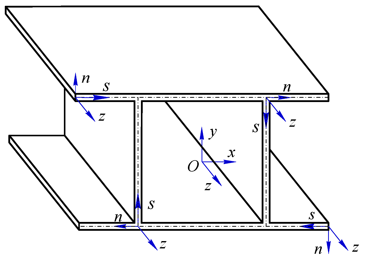
2.1. Displacement Fields

The displacement of a point on the mid-surface of the cross-section is defined with the axial u, tangential v and normal w components, which are prescribed to be positive along the axial direction of the local coordinate system (n, s, z) adopted for each wall. In addition, a global coordinate system (x, y, z) is set with its origin located in the centroid of the cross-section at one end of the structure. The two coordinate systems are shown in Figure 1.
The displacement of an arbitrary point on the structure is described with three components of U, V and W in the global coordinate system. By considering both the membrane and flexural behaviors of the plate, the displacement field, D = [U, V, W], is obtained as
U ( n , s , z ) = u ( s , z ) n w , s ( s , z ) , V ( n , s , z ) = v ( s , z ) n w , s ( s , z ) , W ( n , s , z ) = w ( s , z ) ,
where a subscript comma denotes differentiation with respect to the following variable. Here, the components, v and w, are in-plane (sn plane) displacements and u is the out-of-plane displacement. By separating the variable dependencies on the s (over the cross-section) and z (along the longitudinal axis) dimensions, these components on the mid-surface are approximated through a set of independent basis functions defined along the coordinate s as
u ( s , z ) = k = 1 N 1 ϕ k ( s ) χ k ( z ) , v ( s , z ) = h = 1 N 2 ψ h ( s ) χ N 1 + h ( z ) , w ( s , z ) = h = 1 N 2 ω h ( s ) χ N 1 + h ( z ) ,
where the subscripts k and h are the numbers of out-of-plane and in-plane deformation modes, respectively; φ, ψ, ω are the shape functions of sectional deformation modes on the axial, tangential and normal directions, respectively; and χ is the amplitude function varying along the longitudinal axis, which is also referred to as the generalized displacement. It should be noted that one in-plane mode corresponds to two shape functions ψ and ω, while out-of-plane modes one-to-one match shape functions φ.
Substitute Equation (2) into Equation (1), and the three-dimensional displacement D can be written in a one-dimensional way with a transformation matrix H as
D ( n , s , z ) = H x = [ φ n ω z 0 ψ n ω , s 0 ω ] { x O x I } ,
where the generalized displacement vector x, spanned by the set of amplitude functions χ, is separated into two column submatrices, xO and xI; the two submatrices correspond to the out-of-plane and in-plane deformation modes, respectively; and φ, ψ and ω are the shape function vectors constituted by the set of φ, ψ and ω, respectively.

2.2. Strain and Stress Fields

The strain and stress fields are obtained under the small displacement hypothesis, which are further written in the Kirchhoff’s formulation as
ε ( n , s , z ) = { ε z z ( n , s , z ) ε s s ( n , s , z ) γ s z ( n , s , z ) } = C D ,
σ ( n , s , z ) = { σ z z ( n , s , z ) σ s s ( n , s , z ) τ s z ( n , s , z ) } = E ε ,
where the compatibility operator C and the constitutive matrix E for the plane stress condition are respectively given by
C = [ z 0 0 0 s 0 s z 0 ] , E = [ E 1 ν 2 E ν 1 ν 2 0 E ν 1 ν 2 E 1 ν 2 0 0 0 E 2 ( 1 + ν ) ] .
Here, E and ν are the material Young’s modulus and Poisson’s ratio, respectively.
Substituting Equations (3) and (6) into Equations (4) and (5) yields
ε ( n , s , z ) = [ φ z n ω 2 z 2 0 ψ , s n ω , s s φ , s ( n ω , s + ψ n ω , s ) z ] { x O x I } ,
σ ( n , s , z ) = E 1 + ν [ 1 1 ν φ z 1 1 ν n ω 2 z 2 + ν 1 ν ( ψ , s n ω , s s ) ν 1 ν φ z ν 1 ν n ω 2 z 2 + 1 1 ν ( ψ , s n ω , s s ) 1 2 φ , s 1 2 ( n ω , s + ψ n ω , s ) z ] { x O x I } .

2.3. Beam Governing Equations

The beam energy components are essential for the application of Hamilton’s principle, including the strain energy Ust, the kinetic energy Tkn and the potential energy Upt. By definition, the former two are respectively given by
U st = 1 2 V ε T σ d V ,
T kn = 1 2 V ρ D T t D t d V ,
where V is the beam volume and ρ is the material density. The beam is subjected to distributed loads, being defined with the load vector p = [p, q, r]T. Here p, q and r represent the force densities in the axial, tangential and normal directions, respectively. The potential energy Upt can then be given by
U pt = L A D T p d A d z .
Hamilton’s principle states
δ t 1 t 2 ( T kn U st U pt ) d t = 0 ,
where t1 and t2 are the start time and the end time, respectively.
Substituting Equations (3)–(5) and Equations (9)–(11) into Equation (12) yields
L A δ x T H T ρ H 2 x t 2 d A d z + L A δ x T H T c T E c H x d A d z L A δ x T H T p d A d z = 0 ,
where A and L are the cross-section area and the beam length, respectively. By applying the condition
δ x | t = t 1 = δ x | t = t 2 = 0 ,
Equation (13) becomes
L A ρ φ T φ 2 x O t 2 d A d z + L A E φ T φ x O d A d z + L A G φ , s T φ , s x O d A d z + L A ( E ν φ T ψ , s + G φ , s T ψ ) x I d A d z = L A φ T p d A d z ,
L A ρ n 2 ω T ω 2 x I t 2 d A d z + L A ρ ( ψ T ψ + n 2 ω , s T ω , s + ω T ω ) 2 x I t 2 d A d z + L A E n 2 ω T ω x I ( 4 ) d A d z + L A [ E ν n 2 ω T ω , s s + E ν n 2 ω , s s T ω + G ( 4 n 2 ω , s T ω , s + ψ T ψ ) ] x I d A d z + L A E ( ψ , s T ψ , s + n 2 ω , s s T ω , s s ) x I d A d z + L A ( E ν ψ , s T φ + G ψ T φ , s ) x O d A d z = L A ( ψ T q + ω T r ) d A d z ,
where the superscripts ′ and ″ denote the first and second derivatives with respect to the variable z, respectively; E* = E/(1 − ν2) and G = E/2(1 + ν). Equations (15) and (16) are the governing differential equations of thin-walled structures with a doubly symmetric cross-section.
For the ease of computing, the governing equations are usually interpolated along the longitudinal axis to form one-dimensional finite elements. In view of the two-order partial differential operator in the governing equations, quadratic Lagrange functions are recommended for the interpolation. A special study can be seen in Zhang et al. [26].

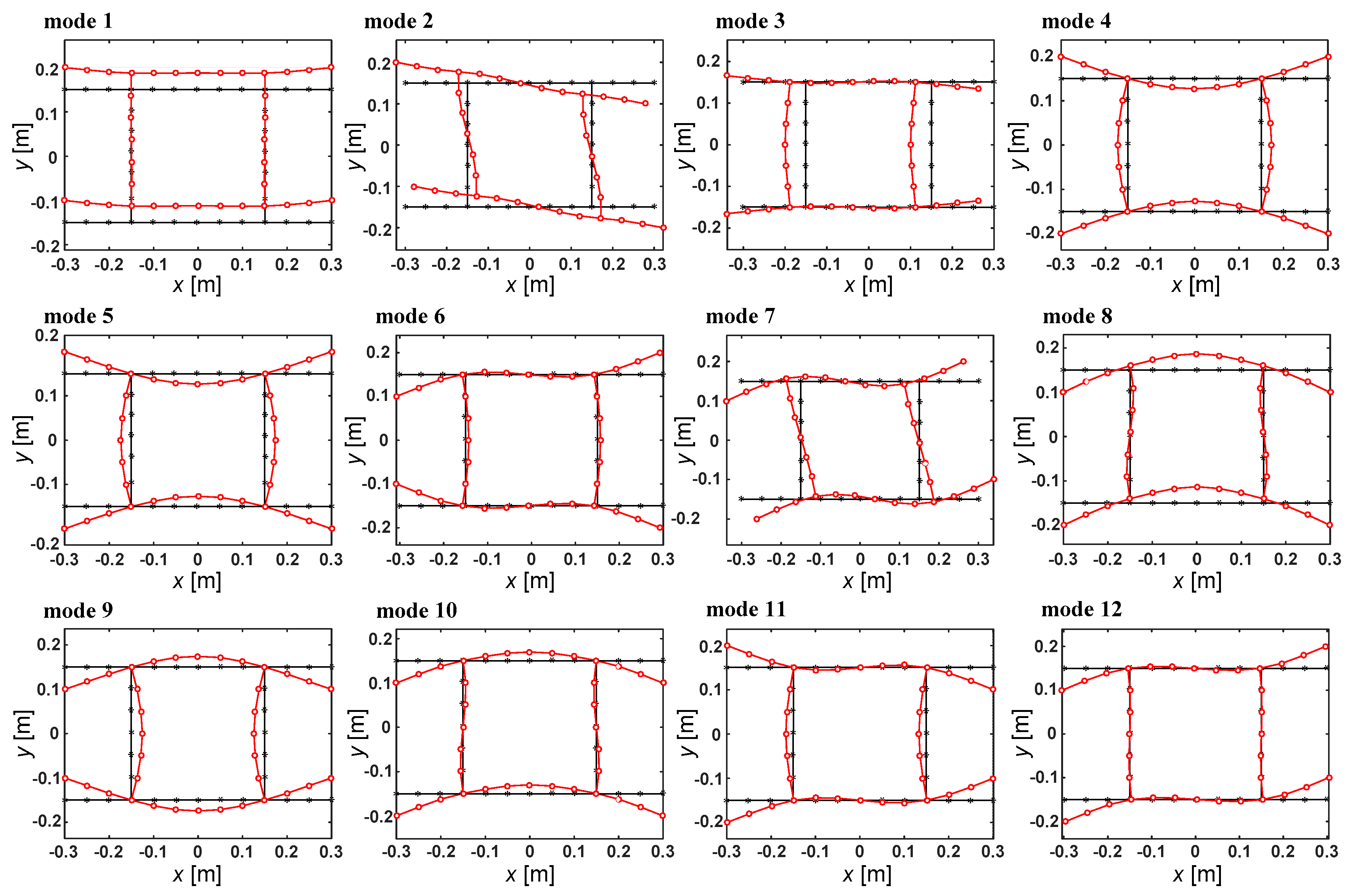
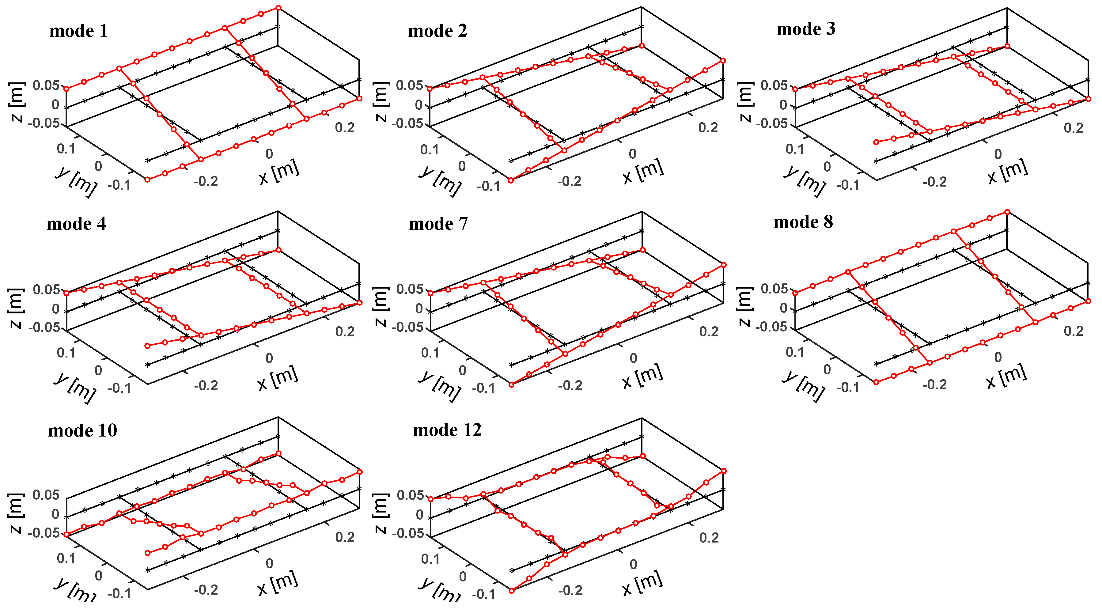
3. Higher-Order Deformation Modes

The procedure to identify sectional deformation modes is begun with the modal analysis based on the shell/plate theory. In this process, the shell-like deformation of the cross-section is presented. The cross-section may be open or closed, with or without branches. Without loss of generality, a thin-walled cross-section possessing all the features above, as shown in Figure 1, is chosen as an example to illustrate the proposed approach.

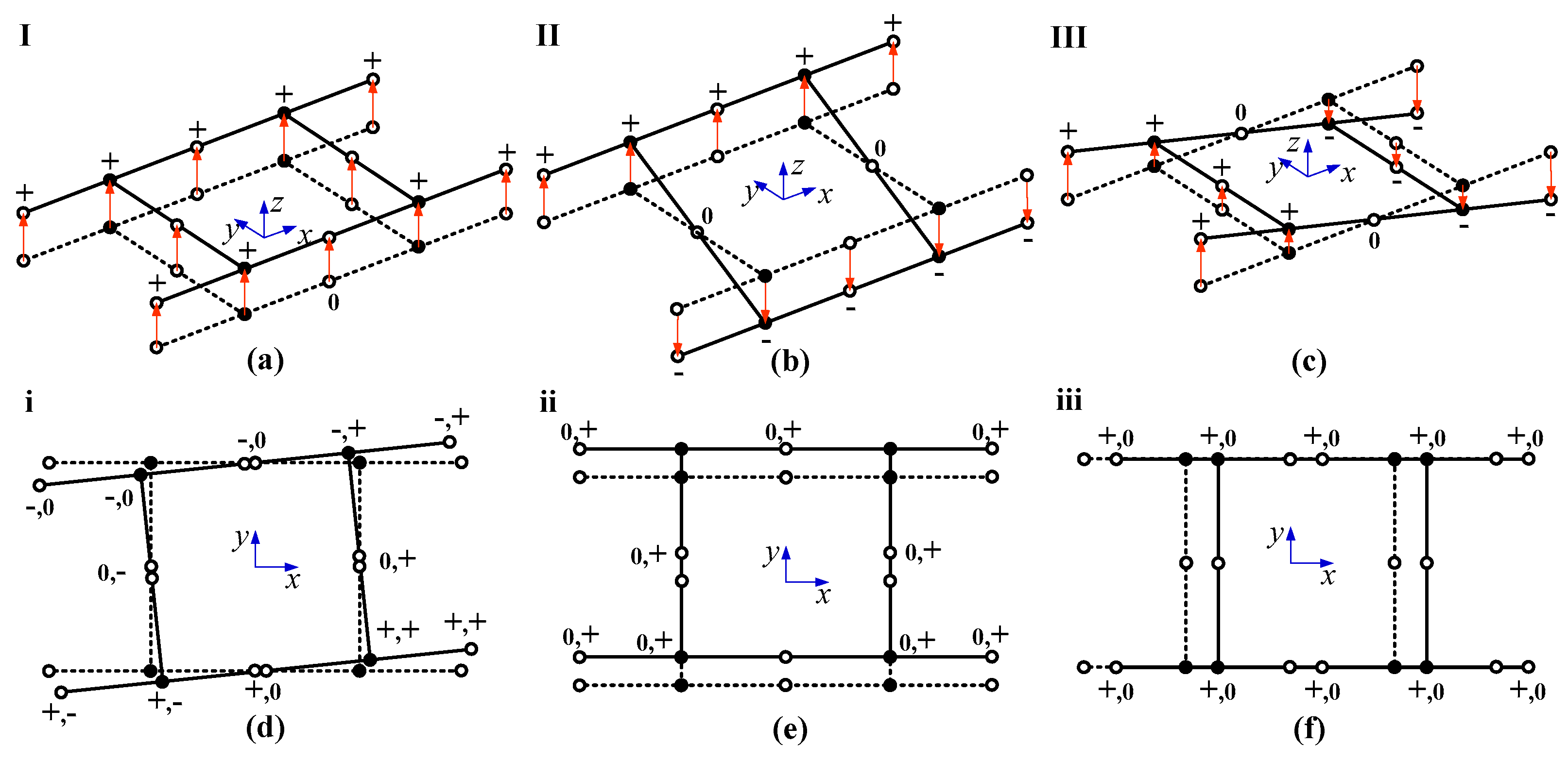
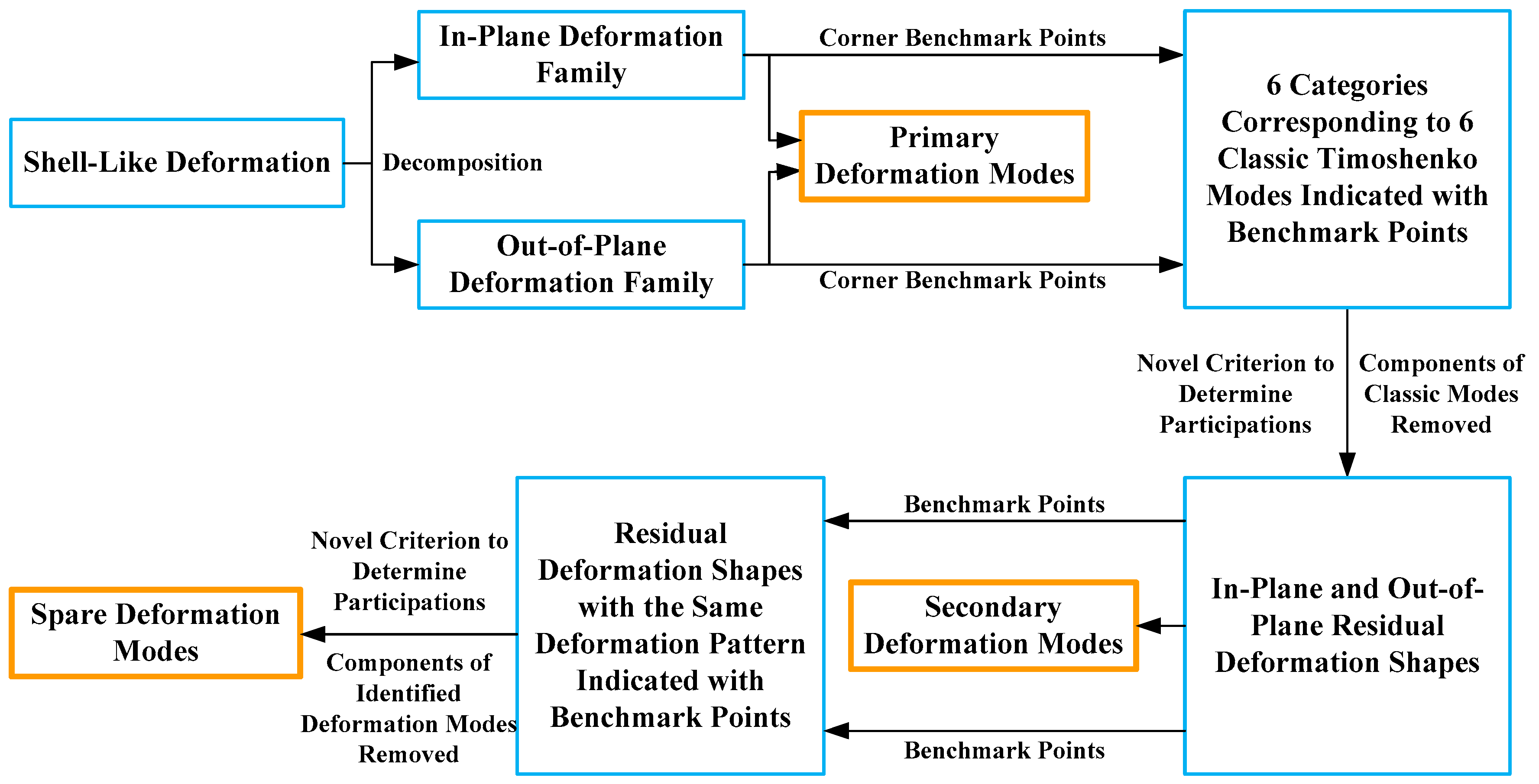
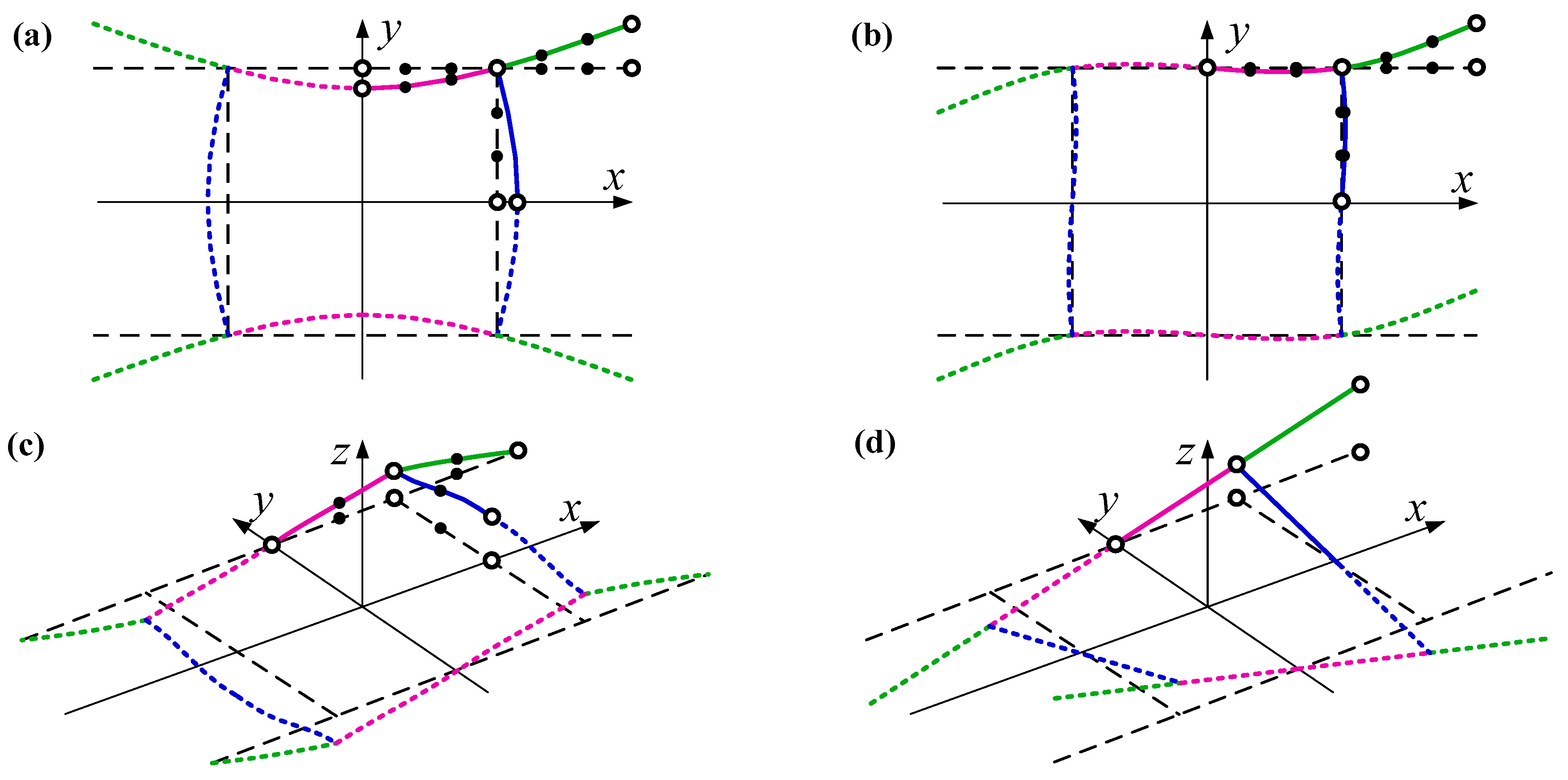
3.1. Shell-Like Deformation

Figure 2 shows a thin-walled structure with a doubly symmetric cross-section. For the convenience of modeling, the structure is fixed at one end with the other end free. Associated geometry and material parameters are set as: section height h = 0.3 m, section width b1 = 0.3 m, flange width b2 = 0.15 m, axial length L = 1.5 m, wall thickness τ = 0.01 m, Young’s modulus E = 2 × 10¹¹ Pa, Poisson’s ratio ν = 0.3 and material density ρ = 7850 kg/m3. It should be pointed out that the choice of these parameters is arbitrary; however, there should be noticeable cross-section deformation.
Since the walls are thin enough, the shell/plate theory is applicable in presenting the shell-like deformation of the cross-section. The shell/plate theory assumes that a mid-surface plane can be used to represent a three-dimensional plate/shell in a two-dimensional form. Currently, the theory has been developed for various shell/plate elements that have been employed in commercial finite element software, such as ANSYS, ABAQUS, ADINA and MSC. ANSYS Shell 181 element is available to be used to model the thin-walled structure in Figure 2. A total of 1080 quadrilateral elements are employed, with 30 elements evenly distributed in the longitudinal direction and 36 over the cross-section. By applying the modal analysis function, the first 12 modal shapes are obtained as the object modes. It should be noted that the number of object modes is related to the number of sectional deformation modes to be identified, which can affect the accuracy of the final one-dimensional model.
Figure 3 presents the deformed contours of the thin-walled structure that have been projected onto the global xy plane. The results show that sectional deformations are dominant for almost every mode shape and that they have become non-negligible factors for the performances of thin-walled structures. In fact, the phenomenon has also been observed in some experiments. For example, noticeable cross-section deformations due to axial and transversal loadings are recreated and exhibited by Debski et al. [27] (see Figure 4) and Ciesielczyk and Studziński [28] (see Figure 5), respectively. In this sense, the conventional beam theory is no longer suitable for these cases. At the same time, it also explains why it is important to study the higher-order deformation of thin-walled structures. Moreover, the sectional deformation modes have been presented, and the next challenge is how to retrieve them.
To obtain these deformation modes, the nodal displacements of the free end cross-section are extracted and decomposed into in-plane (distortion in the xy plane) and out-of-plane (warping vertical to the xy plane, see Carpinteri et al. [29]) components. Figure 6 and Figure 7 exhibit the two deformation mode families, respectively. It should be noted that the out-of-plane family members are not definite before a numerical analysis since not all deformation modes possess out-of-plane components. For example, the z-direction displacements of modes 5, 6, 9 and 11 are almost zero or less than 1/100,000 of the ones along the x- or y-axis. In these cases, the relevant deformation will be passed over. Therefore, only eight out-of-plane deformation modes are obtained from the first 12 modal shapes.
Obviously, those deformed cross-section shapes in Figure 6 and Figure 7 are the superposition of rigid movements of the whole cross-section (classical Timoshenko modes including three translations and three rotations) and sectional elastic deformations (higher-order deformation modes). Since the classical modes have been obtained, the next procedure is pivotal to retrieve the higher-order deformation modes from the modal shapes by removing the components of classical modes.

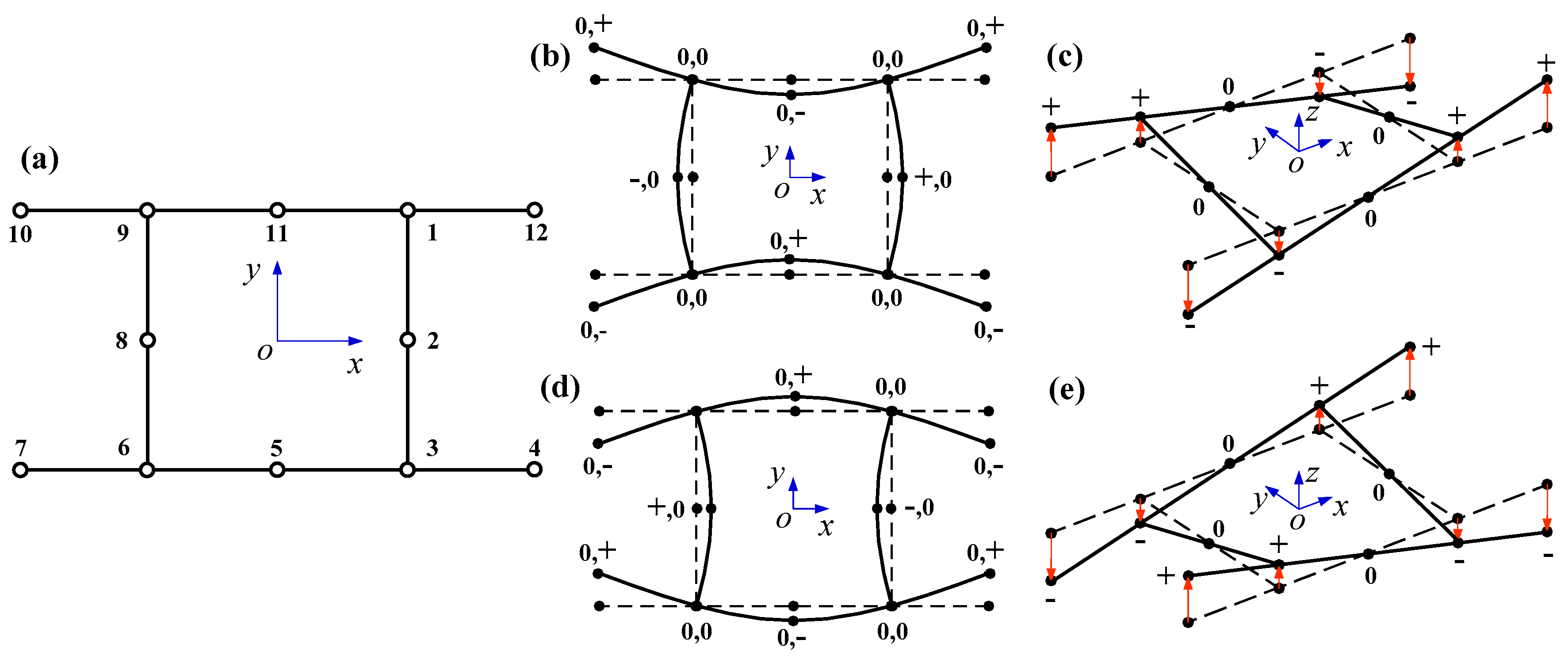
3.2. Benchmark Points

The retrieval of higher-order deformation modes is also mandatory from the view of obtaining a set of sectional deformation modes in hierarchy to form a reduced model. The implementation presupposes the uncoupling of the classical and higher-order modes in the sectional deformation shapes shown in Figure 6 and Figure 7.
For the implementation with a computer, a set of benchmark points are defined on the cross-section to indicate deformation patterns in a digitized way. In other words, each deformation pattern corresponds to a kind of cross-section deformation shapes described with a group of displacement signs stemming from the benchmark points. Therefore, the deformation pattern can indicate whether one sectional deformation mode participates in an object modal shape or not. In Figure 8, 12 benchmark points are set on the corner nodes (points 1, 3, 6 and 9), free end nodes (points 4, 7, 10 and 12) and intermediate nodes (2, 5, 8 and 11). The displacement component of one benchmark point may be one of the three cases: positive (marked as “+”), negative (marked as “-”) or null (marked as “0”). The in-plane deformation modes are expressed with the normal and tangential displacements (two degrees of freedom) of the benchmark points while axial displacements for the out-of-plane modes. In this sense, the 12 benchmark points can identify a total of 3 (number of displacement signs) × 12 (number of benchmark points) × 2 (degrees of freedom) = 72 in-plane modes. Similarly, half of out-of-plane modes can be distinguished since half of degrees of freedom are set for them.
Figure 8b,c show one in-plane and one out-of-plane deformation modes indicated with the deformation signs of benchmark points, respectively. The problem is that two deformation modes, such as the two shown in Figure 8b,d or the two shown in Figure 8c,d, may have opposite displacement components. Essentially, the two forms describe the same deformation mode from the view of the energy method. That is to say, the two forms of deformation modes are equivalent in mechanics. Accordingly, the set of 12 benchmark points can distinguish only half of the sectional deformation modes, namely 36 in-plane modes and 18 out-of-plane ones. In fact, these modes are enough to form a reduced one-dimensional model with a qualified accuracy in most structural analyses.
Moreover, it should be noted that the number of benchmark points needed is related not only to the number of sectional deformation modes to be identified but also to the cross-section configuration. Generally, the corner points and free end points on the cross-section are basic, and a certain number of intermediate points are optional. For example, eight benchmark points may be employed in the cross-section shown in Figure 9a, which can determine 24 in-plane deformation modes and 12 out-of-plane ones. However, the number of benchmark points can be reduced to 4, as shown in Figure 9b, when less sectional deformation modes are needed. In addition, for a cross-section where the lengths of walls vary a lot, some amount of intermediate nodes may be essential to separate the walls into several segments with approximately equal lengths. This measurement is supposed to contribute to the accurate description of the sectional deformation. For example, the I-section in Figure 9c employs two intermediate benchmark points on the web wall, while no intermediate points are introduced in the flange walls of the dual-cell cross-section in Figure 9d. The difference stems from the experience that relatively longer walls usually deform more complexly, where more interpolation nodes are needed to capture the deformation features.

3.3. Identification of Deformation Modes

As shown in Figure 6 and Figure 7, the modal shapes consist of rigid movements of the whole cross-section and the sectional elastic deformation. A novel approach is needed to uncouple them by removing the components of rigid movements of the whole cross-section.
Here, classical Timoshenko modes [30], including three translations and three rotations, are adopted to describe the rigid movements of the cross-section, which are shown in Figure 10. The first three indicate the out-of-plane modes, being numbered as modes I, II and III corresponding to the rotation about z-axis, the translations along y- and x-axis, respectively, while the latter three embody the in-plane ones, which are given the numbers as modes i, ii and iii to represent the extension along z-axis, the rotations about x- and y-axis, respectively. In addition, 12 benchmark points are employed to distinguish these modes for the identification with a computer.
To remove the components of rigid movements of the cross-section, the key is to determine their participations in the sectional deformation shape. Here, a criterion is proposed to uncouple deformation modes in this subsection.

3.3.1. Uncoupling Deformation Modes with a Novel Criterion

The uncoupling is first implemented within each category of sectional deformations. The concept means a group of deformation shapes which contain the components of the same classical Timoshenko mode. In consideration of the doubly symmetric cross-section, the concept can be further simplified to be the deformation patterns indicated with the displacement component signs of the four corner benchmark points (the solid circles in Figure 10). Actually, there are six categories of sectional deformation modes in accordance with the six classical Timoshenko modes. We might as well classify them into categories 1–6 for convenience. In other words, focusing on the four corner benchmark points, if all their nodal displacements along z-, y- or x-axis are with the same values, the corresponding deformation shapes are supposed to belong to category 1, category 5 or category 6, respectively; if the nodal displacements are opposite about x- or y-axis, the corresponding deformation shapes are supposed to belong to category 2 or category 3, respectively; if the nodal displacement components along x- and y-axis are central symmetric about the cross-section centroid, the corresponding deformation shape is supposed to belong to category 4.
Hence, the modal shapes shown in Figure 6 and Figure 7 can be separated into several categories. Among the in-plane family, modes 1, 8 and 10 belong to category 5, modes 2, 7 and 12 belong to category 4, and modes 3, 6 and 11 belong to category 6. In particular, the deformation of modes 4, 5 and 9 are zero on the corner benchmark points, implying no components of classical modes. Among the out-of-plane family shown in Figure 7, modes 1, 8 and 10 belong to category 2, and modes 3 and 4 belong to category 3.
Then, within each category, the participations of classical modes can be determined and removed from the modal shapes. Since the cross-section is doubly symmetric, the process can be implemented just on a quarter of the cross-section. For the categories above except category 4, the process can be carried out with the solution of the following equation:
Θ k Θ k γ Θ c Θ c = Θ i ,   γ = { Θ k ( m , 1 ) Θ c Θ c ( m , 1 ) Θ k ,   for   Θ k ( m , 1 ) 0 ,   Θ k ( m , 2 ) = 0 Θ k ( m , 2 ) Θ c Θ c ( m , 2 ) Θ k ,   for   Θ k ( m , 1 ) = 0 ,   Θ k ( m , 2 ) 0 ,
where ‖‖ means the infinite norm; Θk is the vector constructed by the corresponding nodal displacement components of a deformation shape to be identified; γ is a ratio to guarantee the displacement components of a corner benchmark point to be null after the process; Θc is the vector consisting of nodal displacements of an classical mode; Θi is the vector constituted with the nodal displacements of the newly identified deformation mode, and m is the node number of one corner benchmark point.
For category 4, where both the tangential and normal displacement components are nonzero, another formulation needs to be solved to determine the participation of one sectional mode:
Θ k Θ k γ Θ c Θ c λ Θ r Θ r = Θ i ,   γ = [ Θ k ( m , 1 ) + Θ k ( m , 2 ) ] Θ c [ Θ c ( m , 1 ) + Θ c ( m , 1 ) ] Θ k ,
where Θr is the vector constructed by the nodal displacements of Vlasov distortion [30] and λ is the ratio to guarantee removing the corresponding deformation components.
Actually, a novel criterion has just been expressed in Equations (17) and (18) in uncoupling classical modes and sectional deformation modes. With the process above, the components of sectional rigid movements are removed from the modal shapes, with the residual deformation shapes left to define sectional deformation modes. Furthermore, the process is also useful in the identification of new sectional deformation modes from residual deformation shapes sharing the same deformation pattern. The implementation is to be illustrated in the next subsection.

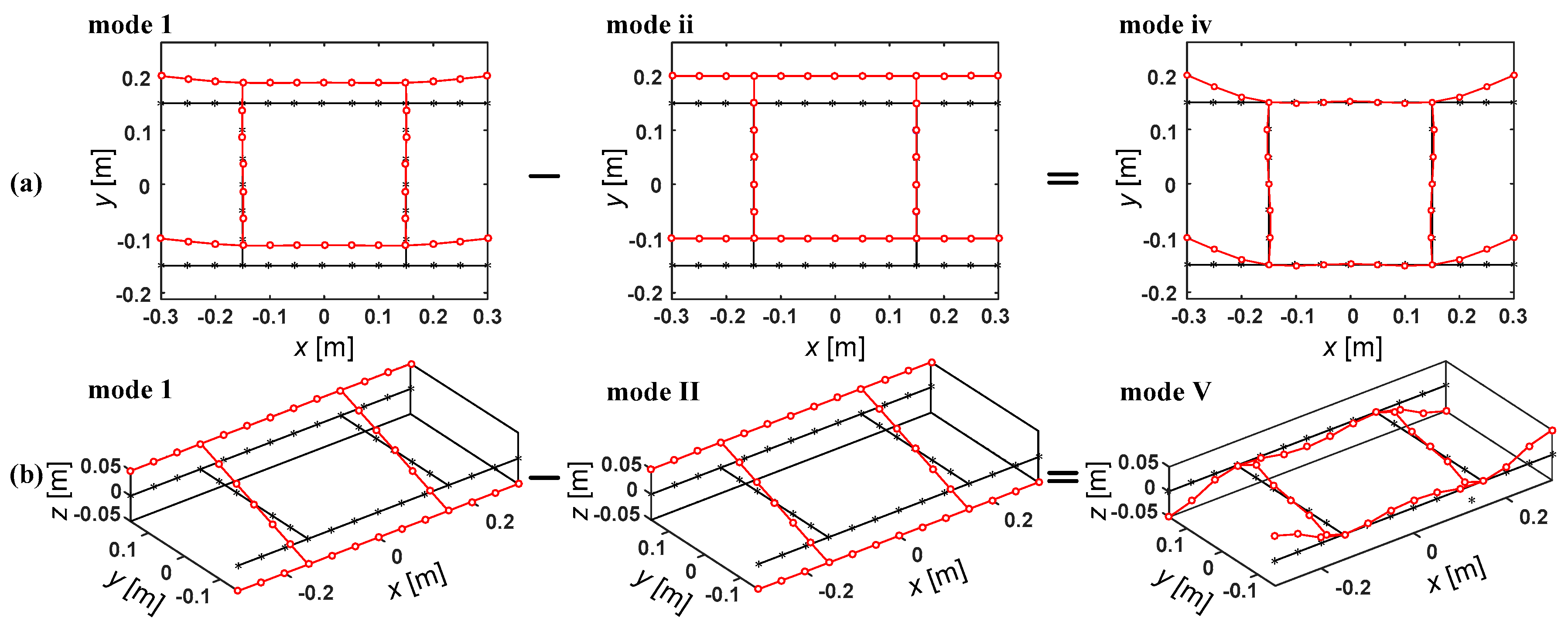
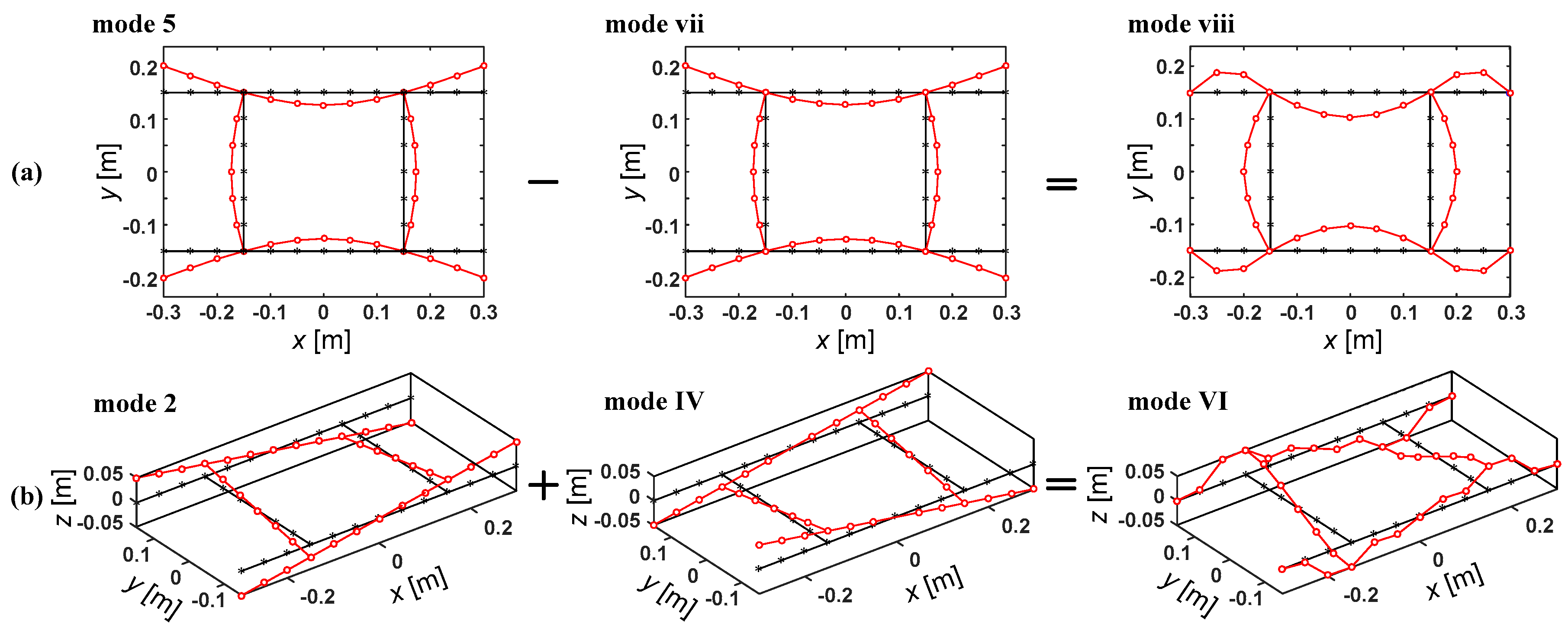
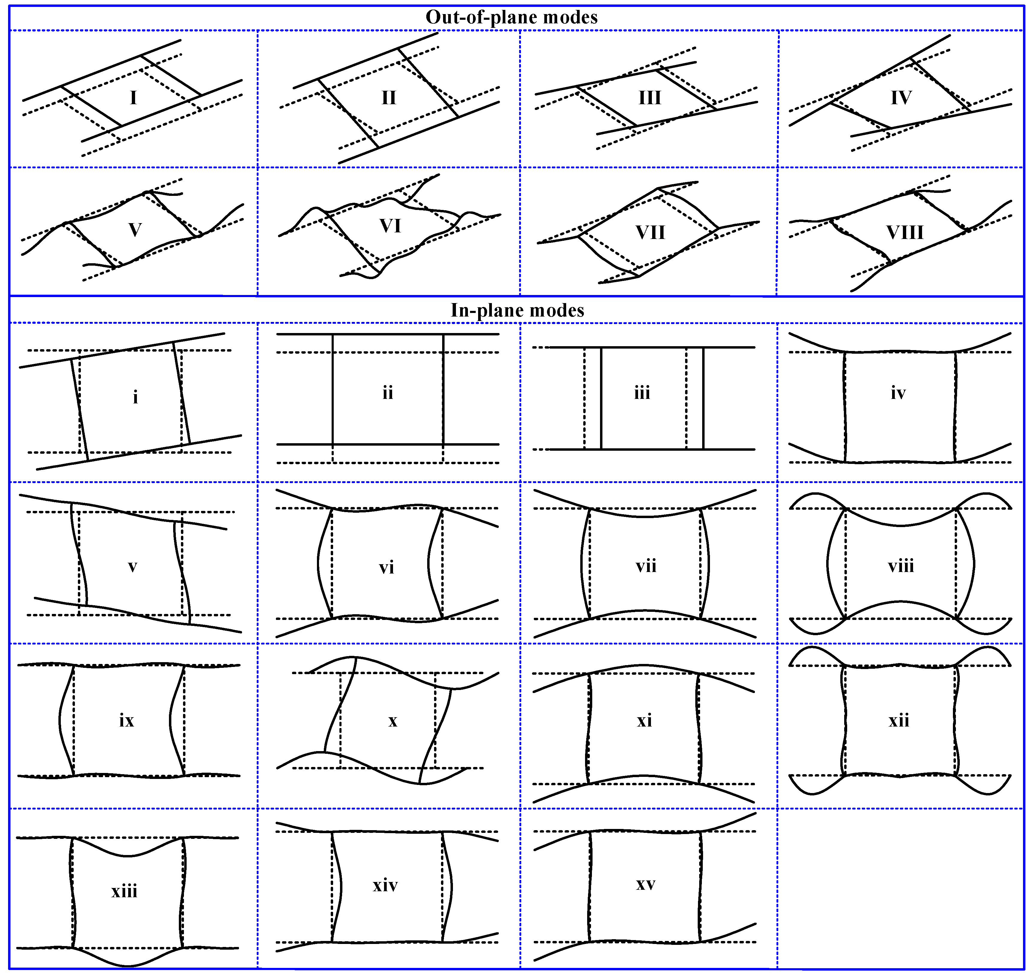
3.3.2. Higher-Order Deformation Modes

The identification of higher-order deformation modes can be classified into three cases, considering the physical interpretation and the clear hierarchy to form a reduced one-dimensional model.
In the first case, the object modal shapes that fall outside of the six categories are directly identified as higher-order deformation modes, which reflect the distortion or warping of the thin-walled cross-section. In modeling a thin-walled structure, these modes play important roles in the improvement of the model accuracy. In this respect, they are classified as the primary deformation modes, next to the classical Timoshenko modes. In the present example, two deformation modes of this kind can be identified, including mode 4 of the in-plane family in Figure 6, and mode 2 of the out-of-plane family in Figure 7.
In the second case, the object modal shapes that fall inside of the six categories are decomposed into the components of classical modes and those of residual deformation shapes, by applying the criterion shown in Equations (17) and (18). The residual deformation shapes can be identified as higher-order deformation modes. Since always working with the classical modes, rather than playing roles independently in a modal shape, they are not vital for the accuracy of a one-dimensional model. Hence, they are classified as the secondary deformation modes, next to the primary ones. For example, within category 5, removing the components of mode iii from the deformation shape of mode 3 yields mode vi, as a secondary mode. Figure 11 demonstrates the whole process, where one in-plane and one out-of-plane secondary deformation modes are identified, respectively.
In the third case, more than one higher-order mode, sharing the same deformation pattern, is identified in the former two cases. These modes are different in physical interpretation, but cannot be distinguished through deformation patterns indicated with the displacement signs of benchmark points. To guarantee their independency, among these residual deformation shapes, the ones derived from a higher order modal will eliminate the components of the one derived from a lower order modal. In this process, the criterion expressed with Equations (17) and (18) should be applied again. The final residual deformation shapes can be identified as new higher-order deformation modes. However, since they are not dominant in any modal shapes, their priority is lower than the secondary modes. Therefore, they are classified as the spare deformation modes. In fact, they can be neglected in a reduced model when the computation efficiency is more significant. Figure 12 has displayed the process, where one in-plane and one out-of-plane spare modes are identified, respectively.
To better exhibit the procedure above, a flow chart is provided in Figure 13, which shows how to uncouple the deformation modes to retrieve primary, secondary and spare deformation modes, respectively. It should be noted that the procedure does not refer to the geometry parameters of the cross-section. However, the double symmetry of the cross-section should be guaranteed since it is essential in the uncoupling of deformation modes by means of the novel criteria. That is to say, the proposed procedure of identifying higher-order deformation modes is general for any doubly symmetric cross-sections.

3.3.3. Shape Functions of Sectional Deformation Modes

To be adopted in the approximation of the displacement field shown in Equation (2), these identified deformation modes need to be described with shape functions in a mathematical way. This process can be carried out by means of the curve fitting technique or the interpolation method. Since the shape functions should be continuous at end nodes of each cross-section wall, the interpolation method is more advisable in this case for the determinacy of passing through one point. Furthermore, the piecewise interpolation is deemed to enhance the capability of capturing the sectional deformation with lower-order polynomials.
As shown in Figure 14, the interpolation is conducted in the first quadrant, actually. Then, the piecewise shape functions for the other three quadrants are completed by applying the symmetry condition. Even in the first quadrant, the interpolation has been separated into three pieces corresponding to the three wall segments. The derived shape function is also related to the number of interpolation nodes to be applied. Generally, the most frequently used interpolation polynomials, namely the linear, quadratic and cubic ones, need two, three and four nodes to determine the unknown coefficients, respectively. Just as shown in Figure 14, the two in-plane modes are interpolated with cubic polynomials, involving four nodes for each segment, while the two out-of-plane modes apply quadratic and linear polynomials, respectively. Naturally, the latter two employ fewer interpolation nodes. It should be pointed out that the two end nodes must be taken into account in the interpolation though a variable number of nodes may be needed for different polynomials. The purpose is to ensure the continuity of the shape function over the whole cross-section.
Although polynomials of any order may be acceptable in describing a sectional mode, some conventional experience still deserves attention. For example, the tangential component of a sectional deformation mode is usually interpolated with a linear polynomial since it usually varies moderately along the cross-section mid-surface, while the normal component needs a cubic function to make its two-order partial derivative with respect to s keep nonzero in the governing equations. As for the axial component, it is always approximated with linear functions in view of the relatively small values compared with the normal ones. However, quadratic or cubic polynomials may also be used in some cases where an in-depth cross-section analysis is in need. For example, the identified deformation modes of the presented cross-section are described with cubic polynomials for the normal and axial components and with linear ones for the tangential component, as shown in Figure 15.

4. Applications and Illustrative Examples

The application of the proposed approach to the presented doubly symmetric cross-section leads to a set of 15 sectional deformation modes, being exhibited in Figure 15. They can be divided into classical modes and higher-order deformation modes, and the latter ones can be further classified into primary, secondary and spare ones according to the way they are identified. By substituting them into the governing equations, a new one-dimensional higher-order model can be obtained for the analysis of thin-walled structures. In this section, numerical studies are carried out to validate the versatility of the new model. Furthermore, for the ease, the thin-walled cross-section in Figure 1 is employed in numerical studies.

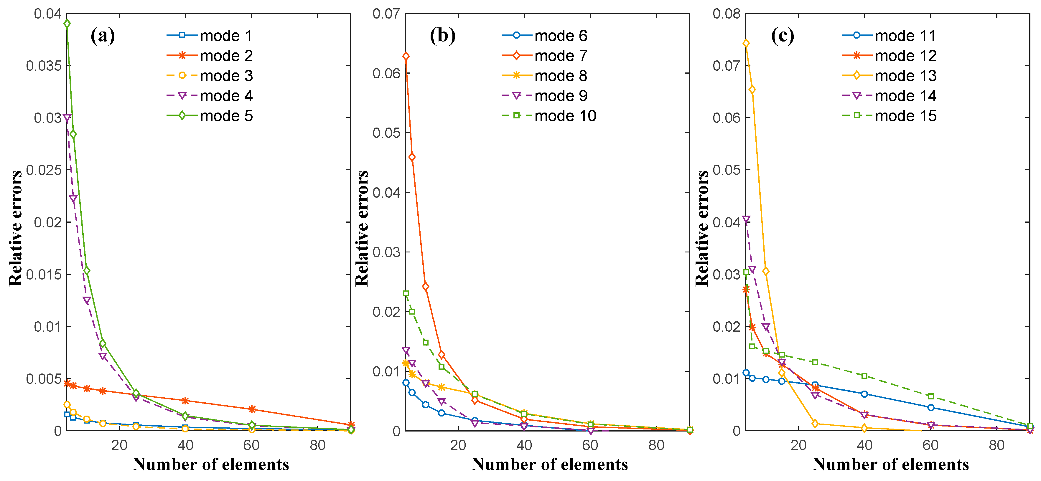
4.1. Convengence of the Finite Element

A quadratic finite element has been developed based on the governing equations, and its convergence is checked in this part. By applying the element in the free vibration analysis of the structure in Figure 2, the relative errors of the first 15 natural frequencies have been demonstrated in Figure 16, varying with the number of employed elements. It should be noted that the structure is meshed equally along the length, and that the converged frequencies are obtained with 100 proposed finite elements, which are considered to become stable.
The presentation reveals that the frequencies of the first 15 modes converge with different rates but finally achieve similar relative errors smaller than 0.1%, when 90 proposed elements are employed. As a consequence, we just employ no fewer than 90 elements in the numerical examples of thin-walled structures.

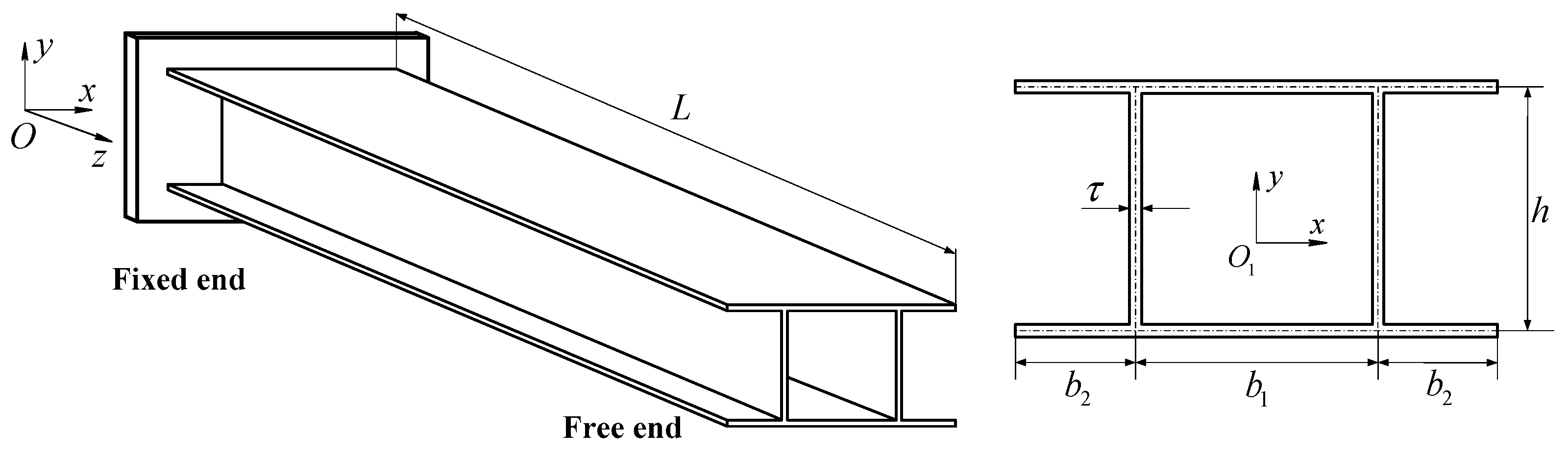
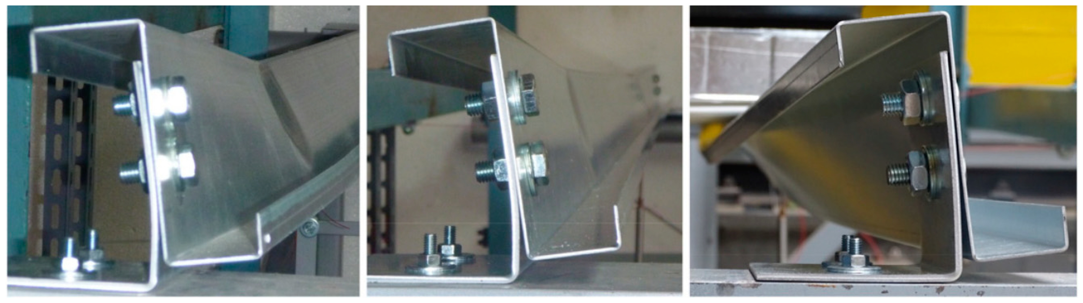
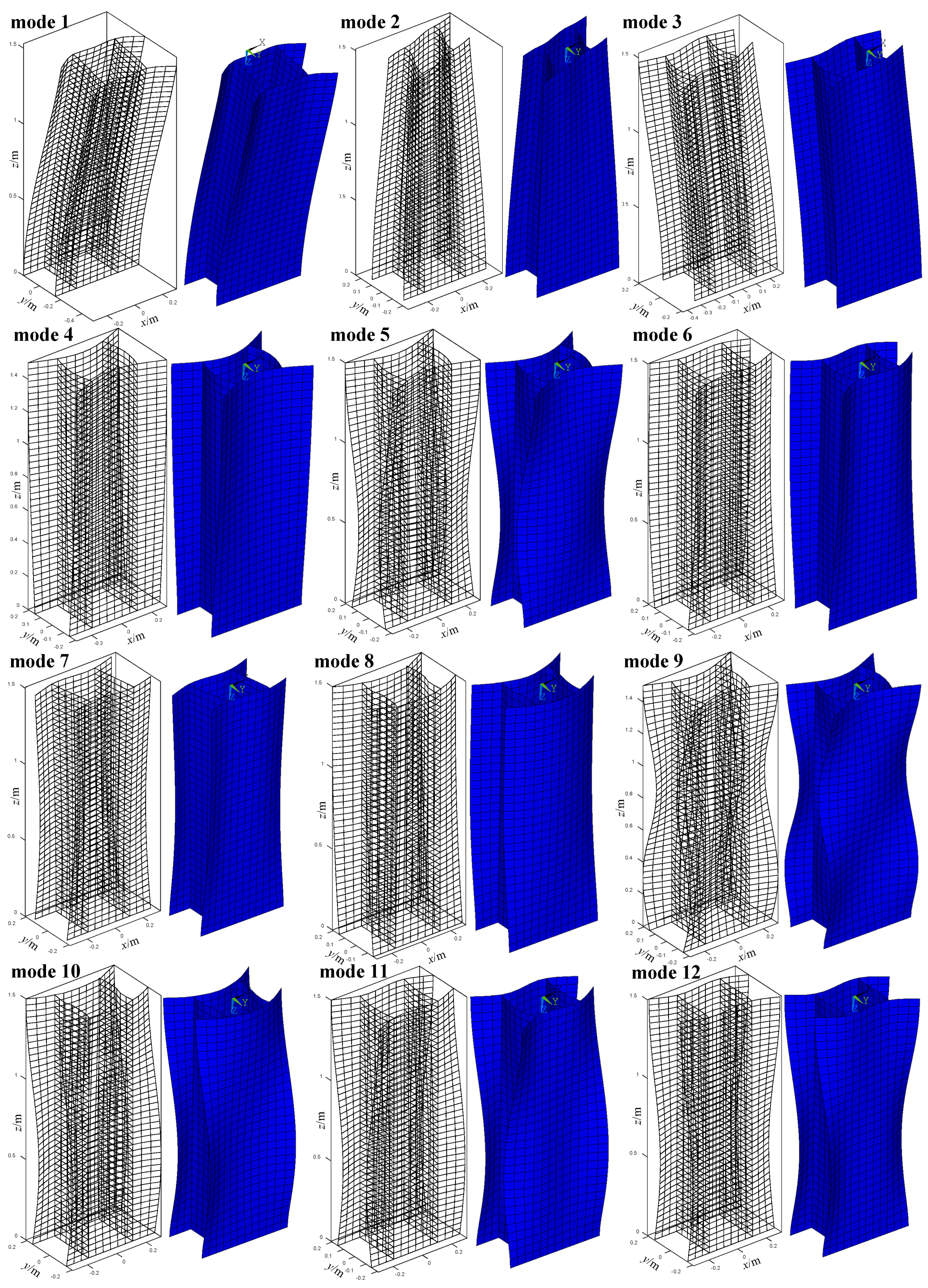
4.2. Case Study 1: A Thin-Walled Structure Fixed at One End

In order to demonstrate the validity and the accuracy of the proposed element, the thin-walled structure with one end fixed and the other end free is considered as the first numerical example. Accordingly, 90 proposed elements are employed to mesh it along the beam axis with an equal length. The results are compared with those of the ANSYS shell model, which consists of 1440 Shell 181 4-node shell elements, distributed as 30 along the length and 48 over the cross-section. Table 1 presents the results about the natural frequencies of the first 15 modes. It should be pointed out that the relative errors are calculated based on the assumption that the results derived from ANSYS shell theory are accurate enough.
The results in Table 1 indicate that the natural frequencies obtained from the proposed model are very close to those from ANSYS shell theory, with relative errors smaller than 4.5%. The results might be not as accurate as those of two- or three-dimensional models, but one should bear in mind that a one-dimensional theory has achieved this with fewer than 1/10 even 1/100 degrees of freedom. It is a great improvement on the computation efficiency. In addition, not any one-dimensional model can predict the first 15 natural frequencies of a thin-walled structure with a similar accuracy. In this sense, the proposed model possesses the advantage of giving balanced consideration both on the precision and the efficiency.
In addition, the longitudinal analysis has also been carried out to prove the hierarchic capability of the identified deformation modes. Since in-plane modes have been specially researched by Zhang et al. [28], this study is focused on the out-of-plane ones. As shown in Figure 17, the amplitudes of these modes (χi in Equation (2)), also known as generalized displacements, fluctuate along the beam axis. Plainly, each modal shape consists of the components of several deformation modes. The most typical case is that a classical mode plays the predominant role with a secondary mode being auxiliary, such as the first, the third, the fourth, the seventh, the ninth and the tenth modes among the first 12 modes. The second case is that the participations of higher-order modes can almost be neglected compared with those of classical modes, such as the fifth, the sixth and the eighth modes. The third case is that the primary modes are dominant with the spare modes playing supplementary roles, such as the second and the eleventh modes. The results confirm that the identified deformation modes possess the hierarchic capability, being able to obtain a reduced model.
Moreover, the proposed model may also have the potential of reproducing three-dimensional behaviors of the thin-walled structure. To check this, the free vibration shapes are analyzed and presented in Figure 18. The results are compared with those of a three-dimensional model based on ANSYS Shell 181. The comparison reconfirms that the proposed model agrees well with ANSYS shell theory. Meanwhile, it is also proved that the presented model can accurately reproduce three-dimensional deformations of the first 12 natural modes, with the higher-order deformation modes identified from the first 12 shell-like deformation shapes.
Actually, with the higher-order deformation modes identified from the first 12 shell-like deformation shapes, the proposed one-dimensional model can also predict higher order mode shapes. In order to validate the idea, the free vibration shapes of the 13th-15th are also studied and presented in Figure 19. The results support the dedication that the proposed model can accurately calculate more modal shapes with fewer sectional deformation modes. It is also a clear proof of the hierarchic capability of the set of the deformation modes.

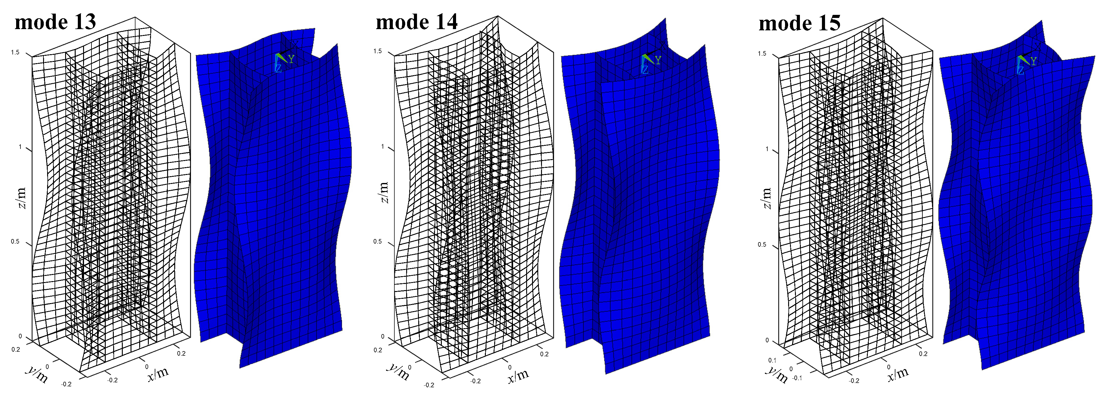
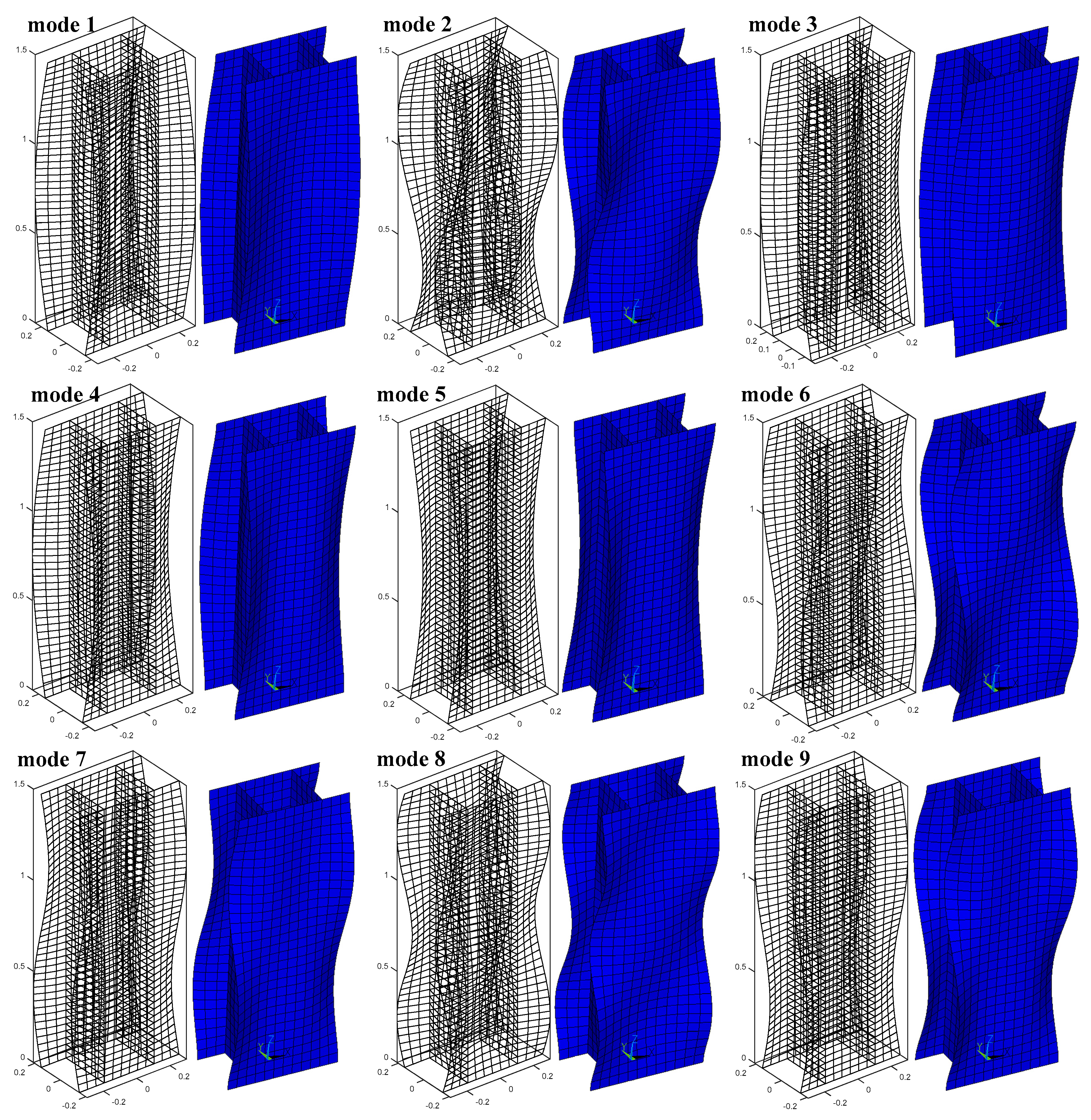
4.3. Case Study 2: A Thin-Walled Structure Fixed at Two Ends

As a next example, the thin-walled structure in Figure 2, being fixed at two ends, is chosen for the free vibration analysis. The example stems from the idea of testing the proposed model with different boundary conditions. One should bear in mind that the set of sectional deformation modes are derived through the cross-section analysis implemented on a cantilevered thin-walled structure; then, whether they are applicable to a structure with different boundary conditions will be very significant for the practicability of the derived model. In fact, they should be equally effective if the set of sectional deformation modes are positively the natural characteristic of the thin-walled cross-section.
Table 2 presents the information about the first 10 modes, consisting of the values of the natural frequencies, obtained with the proposed model and ANSYS shell theory, and the relative errors. Similarly, the data of the proposed model are calculated with 90 quadratic finite elements equally distributed along the axial direction. As a comparison, the ANSYS shell model is discretized into 1120 Shell 181 4-node elements, distributed as 30 elements along the length, and 48 over the cross-section.
The results in Table 2 show that the natural frequencies obtained from the proposed model agree well with those from ANSYS shell theory, with relative errors smaller than 4.5%. The accuracy is similar to that of the cantilevered structure, and even the values of some modes are more accurate than those of the cantilevered structure, such as the first mode. Thus, it can be seen as a preliminary proof of the supposition above.
Furthermore, the capability of reproducing three-dimensional behaviors of the model is checked again, focusing on the modal shapes. Figure 20 provides the comparison concerning the 1st to 9th modal shapes of the fixed-fixed thin-walled structure. The results reconfirm the good agreements with ANSYS shell theory. Hence, it is rational to declare that the proposed model with the same set of sectional deformation modes can accurately reproduce three-dimensional behaviors of thin-walled structures with different boundary conditions. It also embodies the applicability and the generality of the proposed model.

5. Conclusions

The paper focuses on the identification of sectional deformation modes of the doubly symmetric cross-section. The plate/shell theory is utilized to present the shell-like deformation shapes of a thin-walled structure, which are further uncoupled by applying a proposed criterion, with residual deformation shapes left. By introducing benchmark points, these shapes are classified into several deformation patterns, within which the higher-order deformation modes are derived by removing the components of identified ones. By considering the doubly symmetric cross-section, these modes are approximated with shape functions. The identified modes are finally used to formulate the governing equations of the thin-walled structure. The proposed model is examined in numerical examples, and the results validate the accuracy, the efficiency and the practicability of the new model in reproducing three-dimensional behaviors of thin-walled structures. Actually, the authors plan to develop a similar procedure for thin-walled cross-sections with curved walls, by improving the method of approximating the shape functions. In addition, the approach may be also applicative for arbitrary cross-sections, and related study is currently under development.

Author Contributions

Methodology, L.Z.; Project Administration, A.J.; Supervision, A.J.; Visualization, L.P.; Writing—Original Draft, L.Z.; Writing—Review and Editing, W.Z.

Funding

This research was funded by the National Natural Science Foundation of China (Grant No. 51805144), the Foundation of the State Key Laboratory of Mineral Processing (Grant No. BGRIMM-KJSKL-2016-04), the Natural Science Foundation of Jiangsu Province (Grant No. BK20170300), and the Fundamental Research Funds for the Central Universities (Grant No. 2016B14914).

Conflicts of Interest

The authors declare no conflict of interest.

References

  1. Peres, N.; Gonçalves, R.; Camotim, D. GBT-based cross-section deformation modes for curved thin-walled members with circular axis. Thin-Walled Struct. 2018, 127, 769–780. [Google Scholar] [CrossRef]
  2. Carrera, E.; Pagani, A.; Petrolo, M.; Zappino, E. Recent developments on refined theories for beams with applications. Mech. Eng. Rev. 2015, 2, 1400298. [Google Scholar] [CrossRef]
  3. Vlasov, V.Z. Thin-Walled Elastic Beams; Israel Program for Scientific Translations: Jerusalem, Israel, 1961. [Google Scholar]
  4. Yoon, K.; Kim, D.N.; Lee, P.S. Nonlinear torsional analysis of 3D composite beams using the extended St. Venant solution. Struct. Eng. Mech. 2017, 62, 33–42. [Google Scholar] [CrossRef]
  5. Sibileau, A.; García-González, A.; Auricchio, F.; Morganti, S.; Díez, P. Explicit parametric solutions of lattice structures with proper generalized decomposition (PGD). Comput. Mech. 2018, 62, 871–891. [Google Scholar] [CrossRef]
  6. Ghorashi, M. Nonlinear static and stability analysis of composite beams by the variational asymptotic method. Int. J. Eng. Sci. 2018, 128, 127–150. [Google Scholar] [CrossRef]
  7. Carrera, E.; Pagani, A.; Banerjee, J.R. Linearized buckling analysis of isotropic and composite beam-columns by Carrera Unified Formulation and dynamic stiffness method. Mech. Adv. Mater. Struct. 2016, 23, 1092–1103. [Google Scholar] [CrossRef]
  8. Petrolo, M.; Nagaraj, M.H.; Kaleel, I.; Carrera, E. A global-local approach for the elastoplastic analysis of compact and thin-walled structures via refined models. Comput. Struct. 2018, 206, 54–65. [Google Scholar] [CrossRef]
  9. Pagani, A.; Carrera, E. Large-deflection and post-buckling analyses of laminated composite beams by Carrera Unified Formulation. Compos. Struct. 2017, 170, 40–52. [Google Scholar]
  10. Cambronero-Barrientos, F.; Díaz-del-Valle, J.; Martínez-Martínez, J.A. Beam element for thin-walled beams with torsion, distortion, and shear lag. Eng. Struct. 2017, 143, 571–588. [Google Scholar] [CrossRef]
  11. Yu, J.; Hu, S.W.; Xu, Y.C.; Fan, B. Coupled mechanism on interfacial slip and shear lag for twin-cell composite box beam under even load. J. Mech. 2018, 34, 601–616. [Google Scholar] [CrossRef]
  12. Lim, T.K.; Kim, J.H. Thermo-elastic effects on shear correction factors for functionally graded beam. Compos. Part B-Eng. 2017, 123, 262–270. [Google Scholar] [CrossRef]
  13. Akgöz, B.; Civalek, Ö. Effects of thermal and shear deformation on vibration response of functionally graded thick composite microbeams. Compos. Part B-Eng. 2017, 129, 77–87. [Google Scholar] [CrossRef]
  14. Lacidogna, G. Tall buildings: Secondary effects on the structural behaviour. Proc. Inst. Civ. Eng.-Struct. Build. 2017, 170, 391–405. [Google Scholar] [CrossRef]
  15. Tuysuz, O.; Altintas, Y. Time-domain modeling of varying dynamic characteristics in thin-wall machining using perturbation and reduced-order substructuring methods. J. Manuf. Sci. Eng.-Trans. ASME 2018, 140, 011015. [Google Scholar] [CrossRef]
  16. de Lacalle, L.N.L.; Viadero, F.; Hernández, J.M. Applications of dynamic measurements to structural reliability updating. Probab. Eng. Mech. 1996, 11, 97–105. [Google Scholar] [CrossRef]
  17. Zhou, J.; Wen, S.; Li, F.; Zhu, Y. Coupled bending and torsional vibrations of non-uniform thin-walled beams by the transfer differential transform method and experiments. Thin-Walled Struct. 2018, 127, 373–388. [Google Scholar] [CrossRef]
  18. Schardt, R. Eine erweiterung der technischen biegetheorie zur berechnung prismatischer faltwerke. Der Stahlbau 1966, 35, 161–171. [Google Scholar]
  19. Schardt, R. Lateral torsional and distortional buckling of channel-and hat-sections. J. Constr. Steel Res. 1994, 31, 243–265. [Google Scholar] [CrossRef]
  20. Davies, J.M.; Leach, P.; Heinz, D. Second-order generalised beam theory. J. Constr. Steel Res. 1994, 31, 221–241. [Google Scholar] [CrossRef]
  21. Silvestre, N.; Camotim, D.; Silva, N.F. Generalized beam theory revisited: From the kinematical assumptions to the deformation mode determination. Int. J. Struct. Stab. Dyn. 2011, 11, 969–997. [Google Scholar] [CrossRef]
  22. Martins, A.D.; Camotim, D.; Gonçalves, R.; Dinis, P.B. Enhanced geometrically nonlinear generalized beam theory formulation: Derivation, numerical implementation, and illustration. J. Eng. Mech. 2018, 144, 04018036. [Google Scholar] [CrossRef]
  23. de Miranda, S.; Madeo, A.; Melchionda, D.; Patruno, L.; Ruggerini, A.W. A corotational based geometrically nonlinear Generalized Beam Theory: Buckling FE analysis. Int. J. Solids Struct. 2017, 121, 212–227. [Google Scholar] [CrossRef]
  24. Vieira, R.F.; Virtuoso, F.B.E.; Pereira, E.B.R. Buckling of thin-walled structures through a higher order beam model. Comput. Struct. 2017, 180, 104–116. [Google Scholar] [CrossRef]
  25. Vieira, R.F.; Virtuoso, F.B.; Pereira, E.B.R. A higher order model for thin-walled structures with deformable cross-sections. Int. J. Solids Struct. 2014, 51, 575–598. [Google Scholar] [CrossRef]
  26. Zhang, L.; Zhu, W.; Ji, A.; Peng, L. A simplified approach to identify sectional deformation modes of thin-walled beams with prismatic cross-sections. Appl. Sci. 2018, 8, 1847. [Google Scholar] [CrossRef]
  27. Debski, H.; Teter, A.; Kubiak, T.; Samborski, S. Local buckling, post-buckling and collapse of thin-walled channel section composite columns subjected to quasi-static compression. Compos. Struct. 2016, 136, 593–601. [Google Scholar] [CrossRef]
  28. Ciesielczyk, K.; Studziński, R. Experimental and numerical investigation of stabilization of thin-walled Z-beams by sandwich panels. J. Constr. Steel Res. 2017, 133, 77–83. [Google Scholar]
  29. Carpinteri, A.; Lacidogna, G.; Nitti, G. Open and closed shear-walls in high-rise structural systems: Static and dynamic analysis. Curved Layer. Struct. 2016, 3, 154–171. [Google Scholar] [CrossRef]
  30. Zhu, Z.; Zhang, L.; Shen, G.; Cao, G. A one-dimensional higher-order theory with cubic distortional modes for static and dynamic analyses of thin-walled structures with rectangular hollow sections. Acta Mech. 2016, 227, 2451–2475. [Google Scholar] [CrossRef]
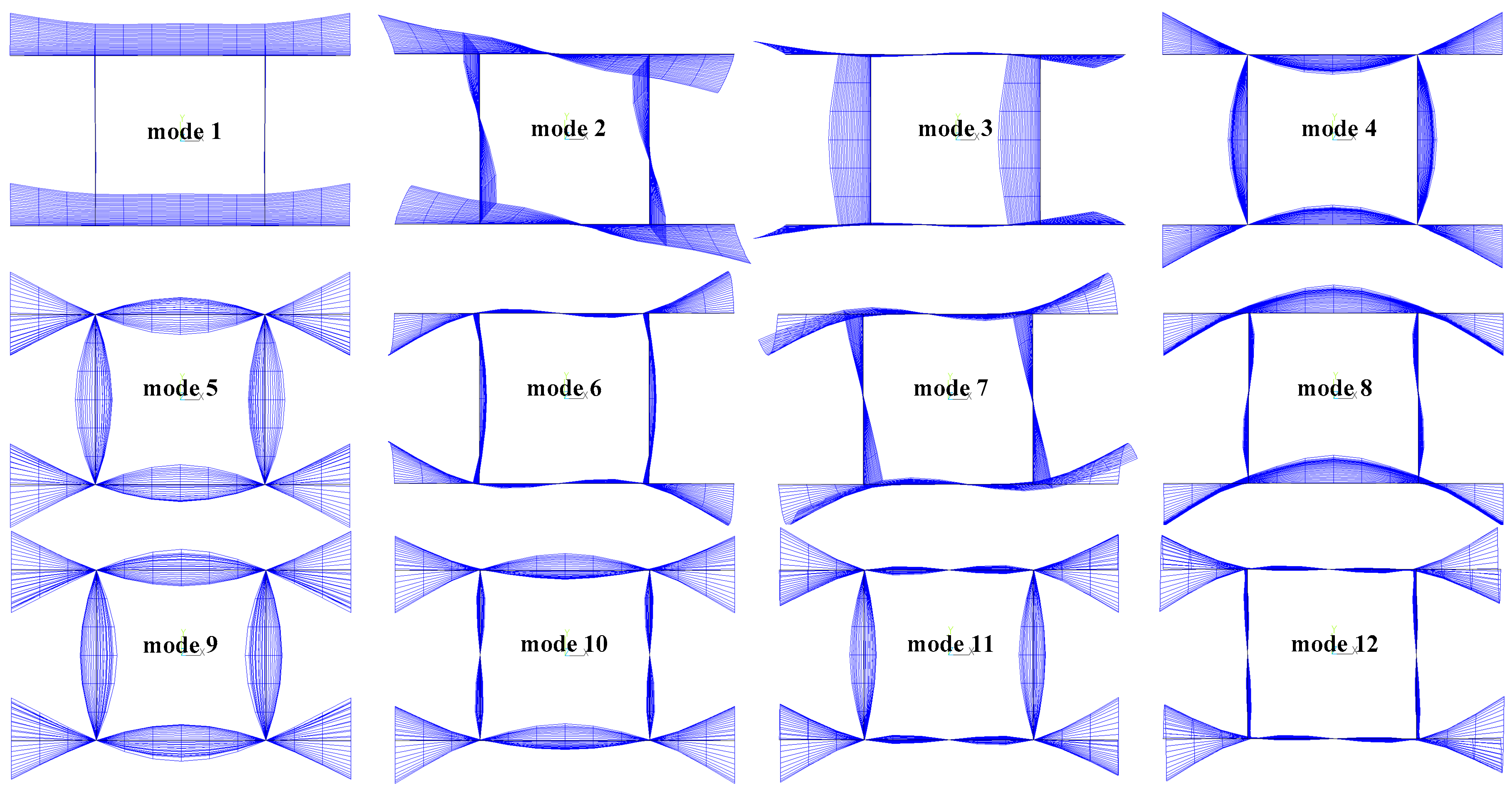
Figure 1. The global (x, y, z) and local (s, n, z) coordinate systems of the thin-walled structure with a doubly symmetric cross-section.
Symmetry 10 00759 g001
Figure 2. A cantilevered thin-walled structure with a branched, doubly symmetric cross-section.
Symmetry 10 00759 g002
Figure 3. Axial projections of the first 12 modal shapes of the thin-walled structure with a branched, doubly symmetric cross-section.
Symmetry 10 00759 g003
Figure 4. Deformation of the thin-walled structure with a channel section under axial loading.
Symmetry 10 00759 g004
Figure 5. Deformation of the Z-section thin-walled structure under transversal loading.
Symmetry 10 00759 g005
Figure 6. In-plane deformation mode family retrieved from the first 12 modal shapes of the thin-walled structure with a branched, doubly symmetric cross-section.
Symmetry 10 00759 g006
Figure 7. Out-of-plane deformation mode family retrieved from the first 12 modal shapes of the thin-walled structure with a branched, doubly symmetric cross-section.
Symmetry 10 00759 g007
Figure 8. Benchmark points on the doubly symmetric cross-section: (a) 12 benchmark points; (b) one in-plane mode and (c) one out-of-plane mode indicated with benchmark points; (d) equivalent form of the in-plane mode shown in (b); (e) equivalent form of the out-of-plane mode shown in (c).
Symmetry 10 00759 g008
Figure 9. Benchmark points for different thin-walled cross-sections: (a) eight benchmark points and (b) four benchmark points for a rectangular cross-section; (c) eight benchmark points for the I-section; and (d) nine benchmark points for a dual-cell cross-section.
Symmetry 10 00759 g009
Figure 10. Classical modes indicated with benchmark points, numbered as modes I, II, III for the out-of-plane ones and modes i, ii, iii for the in-plane ones: (a) rotation about z-axis; (b) translation along y-axis; (c) translation along x-axis; (d) extension along z-axis; (e) rotation about x-axis and (f) rotation about y-axis.
Symmetry 10 00759 g010
Figure 11. Deriving the secondary deformation modes for the doubly symmetric thin-walled cross-section: (a) in-plane mode iv from in-plane mode 1; (b) out-of-plane mode V from out-of-plane mode 1.
Symmetry 10 00759 g011
Figure 12. Deriving the spare deformation modes for the doubly symmetric thin-walled cross-section: (a) mode viii from mode 5; (b) mode xiii from mode 10.
Symmetry 10 00759 g012
Figure 13. The flowchart providing a brief view of the process involved in uncoupling higher-order deformation modes of the doubly symmetric thin-walled cross-section.
Symmetry 10 00759 g013
Figure 14. Interpolation of the shape functions of the doubly symmetric thin-walled cross-section: (a) one in-plane mode in symmetry and (b) one in-plane mode in anti-symmetry described with cubic functions, respectively; (c) one out-of-plane mode in symmetry described with quadratic functions; (d) one out-of-plane mode in anti-symmetry described with linear functions.
Symmetry 10 00759 g014
Figure 15. The shape functions of the identified out-of-plane and in-plane higher-order deformation modes of the doubly symmetric thin-walled cross-section.
Symmetry 10 00759 g015
Figure 16. Convergence of the first 15 natural frequencies of the thin-walled structure varying along with the number of employed proposed elements: (a) the 1st-5th modes; (b) the 6th-10th modes and (c) the 11th-15th modes.
Symmetry 10 00759 g016
Figure 17. Longitudinal variations of generalized displacements of the thin-walled structure in free vibration analyses.
Symmetry 10 00759 g017
Figure 18. Comparison of free vibration shapes of the cantilevered thin-walled structure between ANSYS shell model (right) and proposed model (left) concerning the first 12 modes.
Symmetry 10 00759 g018
Figure 19. Comparison of free vibration shapes of the cantilevered thin-walled structure between ANSYS shell model (right) and proposed model (left) concerning the 13th–15th modes.
Symmetry 10 00759 g019
Figure 20. Comparison of free vibration shapes of the fixed-fixed thin-walled structure between ANSYS shell model (right) and proposed model (left) concerning the first nine modes.
Symmetry 10 00759 g020
Table 1. Natural frequencies of the first 15 modes of the cantilevered thin-walled structure.
ModePresent Model [Hz]ANSYS Shell [Hz]Relative Errors [%]
1st145.63140.383.74
2nd178.26171.893.71
3rd181.35175.633.26
4th183.62185.45−0.99
5th207.44215.37−3.68
6th256.86262.87−2.29
7th257.87263.73−2.22
8th262.62263.86−0.47
9th263.46270.28−2.52
10th274.70277.07−0.86
11th279.30278.060.45
12th297.71309.49−3.81
13th310.89324.74−4.26
14th312.69324.75−3.71
15th332.30346.36−4.06
Table 2. Natural frequencies of the first 10 modes of the fixed-fixed thin-walled structure.
ModePresent Model (Hz)ANSYS Shell (Hz)Relative Errors (%)
1st192.92199.38−3.24
2nd236.09247.04−4.43
3rd251.2262.52−4.31
4th261.05264.38−1.26
5th272.95285.35−4.35
6th290.23303.77−4.46
7th290.85303.95−4.31
8th309.11319.79−3.34
9th321.77335.58−4.12
10th351.7367.43−4.28

