Classification of Two Dimensional Cellular Automata Rules for Symmetric Pattern Generation

Abstract

Cellular automata (CA) are parallel computational models that comprise of a grid of cells. CA is mainly used for modeling complex systems in various fields, where the geometric structure of the lattices is different. In the absence of a CA model to accommodate different types of lattices in CA, an angle-based CA model is proposed to accommodate various lattices. In the proposed model, the neighborhood structure in a two dimensional cellular automata (2D-CA) is viewed as a star graph. The vertices of the proposed graph are determined by a parameter, angle $\left(\theta \right)$. Based on the angle $\left(\theta \right)$, the neighborhood of the CA, which is treated as the vertices of the graph, varies. So this model is suitable for the representation of different types of two dimensional lattices such as square lattice, rectangular lattice, hexagonal lattice, etc. in CA. A mathematical model is formulated for representing CA rules which suit for different types of symmetric lattices. The star graph representation helps to find out the internal symmetries exists in CA rules. Classification of CA rules based on the symmetry exists in the rules, which generates symmetric patterns are discussed in this work.

1. Introduction

Cellular automata (CA) [1] are computational model which consists of a grid of cells where each of the cells acts as a finite automaton. The neighborhood of a cell $C_{ij}$ in a two dimensional CA is the set of surrounding cells on which the updation of $C_{ij}$ depends upon. The updation of each cell is based on a transition function, which is called a rule of the CA. Data are represented as states of the cell in a CA. The states of each cell get updated in unit time steps in parallel, based on rules which are characterized by the neighborhood in synchronous fashion. The states of the CA get updated by the application of rules uniformly in each cell in the CA and it produces patterns at each time step. The output pattern of the CA shows the dynamic and complex behavior. One of the reasons for the complex behavior of the CA is due to the various properties exists in the CA rules. The pattern generated by the CA is the cumulative observation of the output of the CA in successive time steps.

Cellular automata have enormous applications in various domains such as engineering, physics, biology, etc. CA are used for modeling complex systems [2,3,4,5,6]. This has motivated the interest to do the research on the structure of cellular automata. The major components of the CA are its rules that vary according to the number of states, the size of the neighborhood and the geometric structure of the lattice. Since, CA is used as a computational model to model complex problems; the underlying lattices of the CA are different in shape. The primary objective of this work is to propose a model which can represent various types of symmetric lattices and find out the behavior of the rules characterized by the proposed neighborhood structure. Here the neighborhood of a CA is viewed as a type of star graph, so the rules of the model vary according to the lattice structure and size of the neighborhood. In this proposed work, we classify the rules based on the internal symmetric behavior that exists in the rules, which are leading to a symmetric pattern.

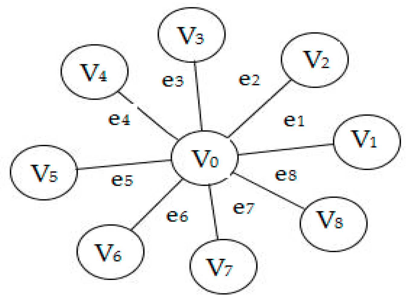
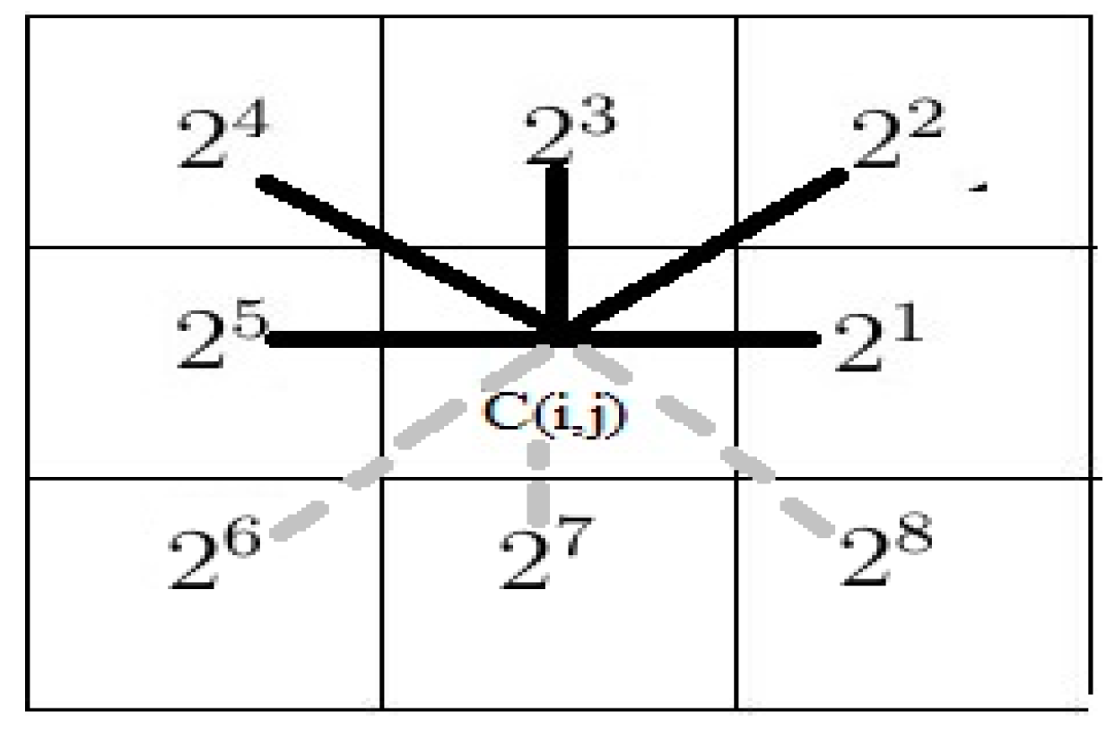
The existing neighborhood structures used in CA are using a fixed neighborhood structure for a specific lattice. Major neighboring structures such as vonNeumann neighborhood [7] contains five neighborhood cells and the Moore neighborhood [8] contains nine neighborhood cells for each cell in a two dimensional CA. Wolfram has done an extensive study on totalistic CA [9] based on two dimensional cellular automata with the Moore neighborhood structure, where the updation of every cell in a CA is based on the sum of the state values of the neighborhood of every cell. A.R. Khan [10] used a different approach to represent rules in a rectangular nine neighborhood CA. In a nine neighborhood CA, fixed positional weight is assigned [10] to each cell in the neighborhood of a cell $C_{ij}$ to indicate the dependency of the neighborhood with the cell $C_{ij}$ to update the cell $C_{ij}$. In Ref. [10] rule 1 indicates the dependency of the cell $C_{ij}$ on itself. Rule 2 indicates the dependency of the cell $C_{ij}$ on its right neighborhood and rule 4 indicate the dependency of the cell $C_{ij}$ on its bottom diagonal cell; rule 8 indicates the dependency of the cell $C_{ij}$ on its bottom cell, etc. in such a way that the nine neighboring cells are considered as nine distinct rules. Figure 1 refers to the two dimensional CA model described in [10] shows the dependency of the neighborhood cells to the cell to be updated, $C_{ij}$. In another approach, two dimensional CA is viewed as a tree [11] with $k+1$ cell structure where each cell has $k$ neighbors. In Ref. [11] the nodes are indexed by numbers $1, 2, 3,.., k$ and the root node is indexed by $\left(k+1\right)$, the rules are defined based on the traditional approach [1]. In order to represent a hexagonal lattice, a seven neighborhood [12] structure is used analogously to a CA model described in [10]. To update a cell in a hexagonal lattice, the dependency of the six surrounding cells [12] on the cell to be updated is considered. In Ref. [12] analogous to the two dimensional model described in [10] positional weight is assigned to each cell in clockwise direction to indicate the dependency of the neighborhood cells on the cells to be updated.

Cellular automata rules have the immense computation power. Depending upon the structure of the neighborhood and the nature of the operations used to define rules [13], the characteristics of the rule may change. In order to find out an exact CA rule for a particular application, we need to classify the CA rules according to its properties. One such property that exists in the CA rule is the internal symmetry exists in it. The output pattern of CA at any iteration varies according to the rule of the CA. The various ways of classification of the rules are discussed in Ref. [14], classification of CA rules into reversible rules, self-symmetric rules and symmetry on pair rules are using matrix algebra on a hexagonal neighborhood model. Linear CA rules are classified based on the patterns generated at $k^{th}$ iteration [15] using fixed positional weight 2D-CA model [10]. Two dimensional CA rules are classified into symmetric rules and nonequivalent rules under black and white $\left(BW\right)$ transformations [11] on the possible permutations in the rule table. Uniform group rules in a two dimensional cellular automata [14] are classified into four classes based on the characteristic matrix called T matrix. Totalistic rules, outer totalistic rules [9] are classified on a 2D-CA based on the number of neighborhoods considered for the updating of each cell.

Symmetry is a property existing in objects; it has a lot of applications [16,17,18,19] in day to day life in various fields. CA is used for modeling complex systems in various domains, in various types of underlying lattices. So a CA model which is capable of generating symmetric patterns helps to model lots of applications [20] in various fields such as architecture, biology, human body, etc. where symmetry plays a vital role. Based on the symmetric nature of the CA rules, one can decide that whether the CA can generate symmetric patterns or not. Various studies exist on symmetry in CA rules based on various methods. Internal symmetries of CA rules based on permutation states [21], β-calculus, and a universal map derived based on β-calculus [22], discrete Walsh analysis [23], and polynomial representation of one dimensional CA [24] symmetropy [25] are the various methods that exist to measure the symmetry of CA rules. If the rule possesses symmetry, it reflects in the output pattern. By modeling symmetric objects in a CA, one can identify the anomalies present in the objects easily based on the symmetric patterns generated from the objects. So, the main objectives of this paper are as follows.

In the absence of a generic CA model to represent various types of lattices, the main objective of this paper is to propose an angle-based CA model to accommodate various types of symmetric lattices and propose a generic mathematical equation to represent CA rules for any symmetric lattice. In this paper, we propose the classification of CA rules based on the amount of the internal symmetries that exists in the CA rules, which will lead to symmetric patterns generated by a CA.

2. Materials and Methods

2.1. Angle-Based Address for Cells in a Lattice

Since one of the objectives of this paper is to represent various types of symmetric lattices using CA, a mechanism is required to accommodate various types of lattice in a CA. A finite lattice is a regular arrangement of objects such as rectangle, circle, hexagon, etc. called a rectangular grid, circular grid, or hexagonal grid, respectively. Here we assume a two dimensional CA with two states. In order to accommodate various types of symmetric lattice, we use polar coordinate system to refer a cell with respect to the cell to be updated. The cell to be updated is considered as the pole and the horizontal line drawn from the pole is the polar axis (initial line). For this purpose, we define the distance of a cell from the pole as the number of cells traversed (other than the cell to be updated) by the line joining the pole and the center of the cell. For example, in a rectangular lattice, the distance of a neighbor cell from the cell to be updated is one unit. In various symmetric lattices, the neighboring cells w.r.t. a pole is arranged at different angles such as $60°$ in a hexagonal lattice, $45°$ in a rectangular lattice, etc. In order to accommodate various symmetric lattices in a two dimensional CA, we define the polar angle ($\Phi$) and input angle ($\theta$) as follows.

Definition 1 (Polar angle ($\Phi$) of a cell).

It is the angle measured in the counter clockwise direction from the reference point (pole) to the center of a neighboring cell in the unit distance in a two dimensional regular lattice.

The reference point is considered as the center of the cell to be updated. The polar angle of each cell varies according to the pole. Every cell will have a unique polar angle w.r.t. a fixed pole.

Definition 2 (Input angle ($\mathbf{\theta }$)).

It is a constant, which is determined by the formula, $\theta =360°/p$, $0<\theta \le 180°$ where $‘p\text{'}$is a positive even integer which produces $\theta$ as a whole number.

Figure 2 shows the addressing of cells w.r.t a cell in a rectangular lattice. We refer a neighboring cell as $C\left(1, \Phi \right)$, as the distance from the cell to be updated $C\left(0, 0\right)$ to a neighboring cell is one unit and $\Phi$ is the polar angle measured between $C\left(0, 0\right)$ and any specific neighboring cell.

In the two dimensional CA, the existing neighborhood structures such as Moore neighborhood and von Neumann neighborhood uses fixed neighborhood size. With an idea of having a flexible number of neighborhoods in any type of symmetric lattice, and to have a general representation of neighborhood, an n-star graph CA (nSG-CA) is proposed to represent the neighborhood structure in a two dimensional CA.

2.2. An n-Star Graph Cellular Automata Model for Two Dimensional CA

Definition 3 (Graph).

A graph is an ordered pair, G = (V, E), where V is the vertex set and E is the edge set [26].

For example, a graph G is shown in Figure 3.

In the graph $G=\left(V,E\right)$, where $V=\left\{V_0,V_1,V_2,V_3,V_4,V_5,V_6,V_7,V_8\right\}$ and

$$E=\left\{e_1=\left(V_0, V_1\right), e_2=\left(V_0,V_2\right), \dots .,e_8=\left(V_0,V_8\right)\right\}$$

Definition 4 (n-star graph).

It is defined as a type of star graph with one internal node and $N$ leaves.

Figure 3 is a sample n-star graph. The vertex set in the n-star graph, $\mathrm{G}$ as shown in Figure 3 is, $\mathrm{V}=\left\{{\mathrm{V}}_0\right\}\mathrm{U}\left\{{\mathrm{V}}_1,{\mathrm{V}}_2,{\mathrm{V}}_3,{\mathrm{V}}_4,{\mathrm{V}}_5,{\mathrm{V}}_6,{\mathrm{V}}_7,{\mathrm{V}}_8\right\}$ and edge set, $\mathrm{E}=\left\{{\mathrm{e}}_1=\left({\mathrm{V}}_0,{\mathrm{V}}_1\right),{\mathrm{e}}_2=\left({\mathrm{V}}_0,{\mathrm{V}}_2\right),\dots ,{\mathrm{e}}_8=\left({\mathrm{V}}_0,{\mathrm{V}}_8\right)\right\}$.

Definition 5 (2D-CA).

It is a two dimensional cellular automata have five tuples, $2DCA=\left(L, S, N_b, N, f\right)$, where:

i. 

$L$ is a two dimensional regular lattice.

ii. 

$S$ is the set of nonempty binary states.

iii. 

$N_b$describes the finite set of neighborhood of each cell$C_{ij}$,$N_b$=$\left\{C_{ij}\right\} U \{N$} and$\left\{C_{ij}\right\}{\displaystyle \cap }\left\{N\right\}=\Phi$where$C_{ij}$is the cell to be updated in a two dimensional lattice,$i$indicates the distance of the cell$C$from the cell to be updated, and$j$indicates the polar angle of the cell$C$with the cell to be updated, so$C_{ij}$is$C\left(0, 0\right)$and$N$is the set of the neighborhood of the cell$C_{ij}$, which excludes cell$C_{ij}$from the set$N_b$.

iv. 

$f$is the transition function, defines the local rule to be applied to each cell,$f:$$S_{t+1}$($C_{ij}$) =$S_t$($C_{ij}$),$S_t$($n_1$),$S_t$($n_2$), …,$S_t$($n_8$), where$S_{t+1}$($C_{ij}$) indicates the successor state of the cell$C_{ij}$at$t+1$time step,$S_t$($C_{ij}$) indicates the current state of the cell$C_{ij}$at$t$time step and$S_t$($n_1$), …,$S_t$($n_8$), indicates the current state of each cell in the neighbourhood of$C_{ij}$.

The neighborhood structure of 2D-CA is can be viewed as one type of a star graph, so it can be called as n-star graph where ‘n’ indicates the neighborhood structure.

Definition 6 (n-Star graph cellular automata model (nSG-CA)).

It is a type of star graph cellular automata, where the cell to be updated and its neighborhood in a two dimensional CA are viewed as an n-star graph,nSG-CA$=\left(L,S, N_b, N,f,V, E\right)$, where:

i. 

L is a regular symmetric lattice where cells are arranged in such a way that, each cell $C_{ij}$ is surrounded by an even number of cells in unit distance.

ii. 

$S$ is the set of binary states.

iii. 

$N_b$describes the finite set of neighborhood of each cell$C_{ij}$in an nSG-CA,$N_b$=$C_{ij}U$$N$and$C_{ij}{\displaystyle \cap }$$N=\Phi$, the cardinality,$\left|N_b\right|$ at every cell position must be odd.

iv. 

$N$is the set of neighborhood cells of each cell$C_{ij}$, excluding the cell$C_{ij}.$

v. 

$f$ is the transition function termed as a rule in nSG-CA which is characterized by the neighborhood as in the definition of 2D-CA.

vi. 

$V$is the set of vertices in the nSG-CA; for each cell in nSG-CA, the cells in the neighborhood$N_b$is mapped into vertices V such that$C_{ij}$is mapped into$V_0$and every element in$N$is mapped into vertices of the n-star graph such that$n_1\to V_1$,$n_2\to V_2, n_3\to V_3, \dots n_N\to V_N$for all$n_i ϵ N$.

vii. 

$E$is the set of edges in the nSG-CA, which is formed by connecting each cell in the neighbourhood with$C_{ij}$such as$\{(V_0, V_1),\{(V_0, V_2),\dots \{(V_0, V_N\left)\right\}.$

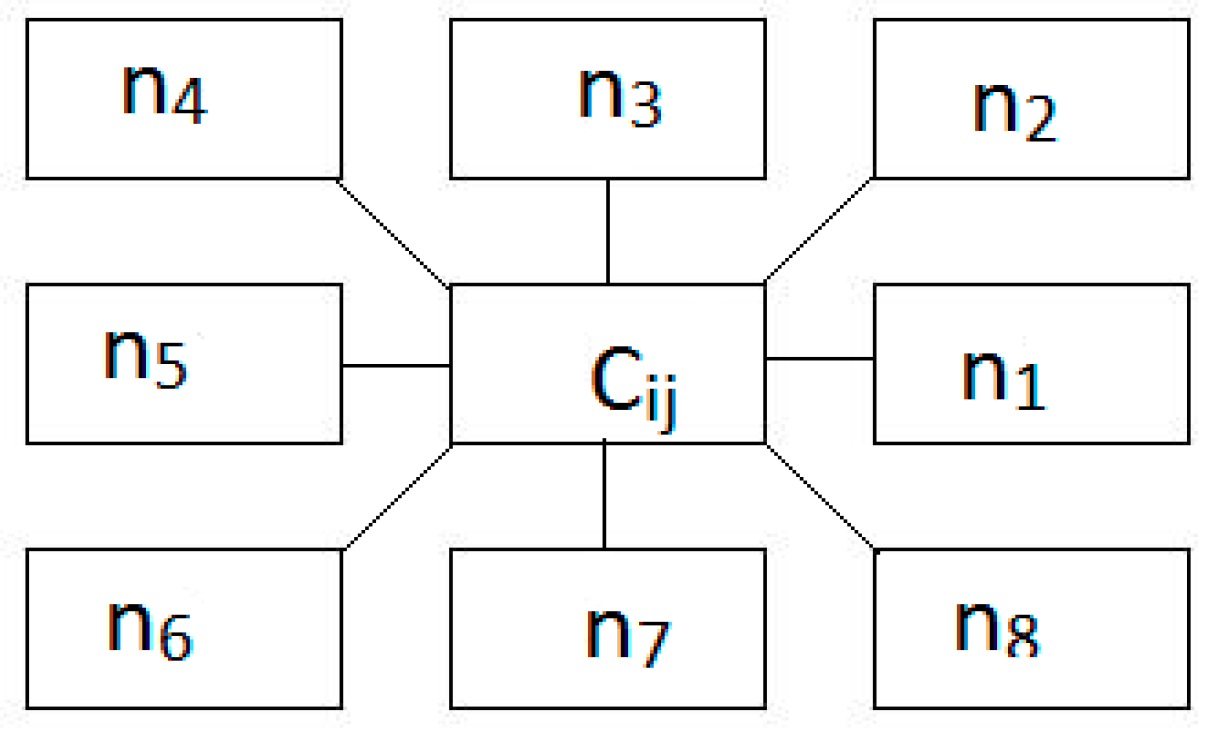
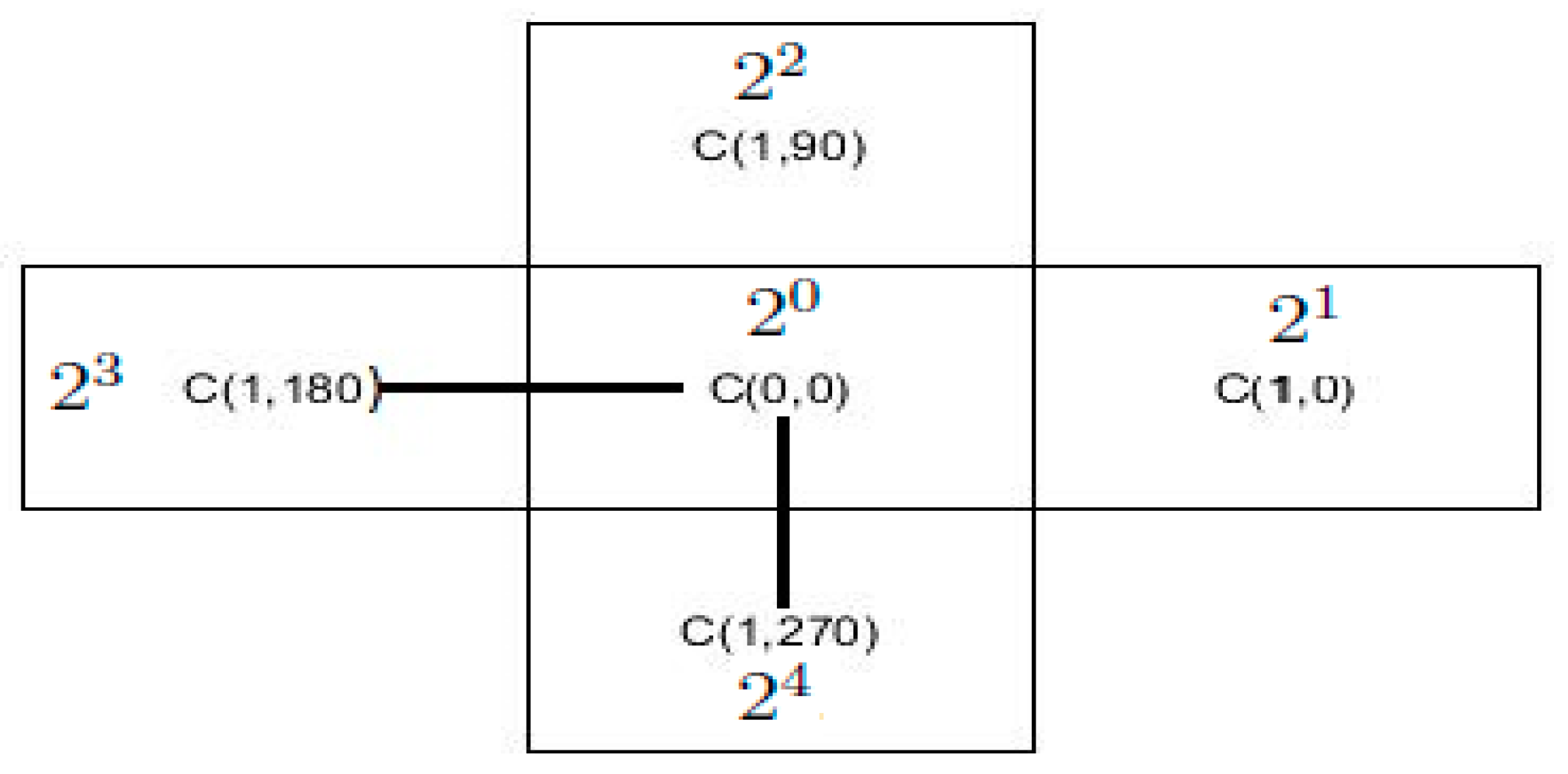
The nSG-CA model for a rectangular lattice with nine neighborhood is shown in Figure 4, where $C_{ij}$ is the cell to be updated and the cells in the neighborhood such as $n_1, n_2, n_3,..., n_8$ are equivalent to:

$$C\left(1,0°\right), C\left(1,45°\right), C\left(1,90°\right),C\left(1,135°\right),C\left(1,180°\right),C\left(1,225°\right),C\left(1,270°\right), C\left(1,315°\right)$$

3. Generic Rule Convention of nSG-CA Model

In a star graph CA, the state of each cell gets updated at every time step based on a rule, which is characterized by the neighborhood. A cell in the neighborhood of $C_{ij}$ is indicated as $n_{ij}$, where $i$ is unit distance and $j$ is $\Phi$, the polar angle of the neighborhood cell. The CA rules are defined based on the dependency of the cell to be updated with the neighboring cells, i.e., the dependency of $C_{ij}$, the cell to be updated with $n_{ij}$, any cell in the neighborhood of $C_{ij}$ is defined as that, the state of $n_{ij}$ at every time step take part in the updation of $C_{ij}.$ The rule may depend on a maximum of $\left|N_b\right|$ cells in a neighborhood structure, which include the cell $C_{ij}$, and its N neighborhood in the unit distance. Different rules are used to update a cell $C_{ij}$, based on the dependency of $C_{ij}$ with its neighbourhood cells.

Since rules are characterized by the neighborhood, every rule can also be represented as a star graph.

In order to distinguish the rules, a positional weight, $P_w$ is assigned to each cell in the neighborhood. The positional weight of each cell $n_{ij}$ in the neighborhood w.r.t the $C_{ij}$, the cell to be updated is determined by the equation,

$$P_w\left(n_{ij}\right)=2^{\left(\left(\frac{\mathsf{\Phi }\left(n_{ij}\right)}{\theta }\right)+1\right)}, n_{ij} ϵ N\left(C_{ij}\right)$$

(1)

where $\Phi$ is the polar angle of each neighborhood cells, $n_{ij}ϵ\mathrm{N}$ with the $C_{ij}$ the cell to be updated. The positional weight, $P_w$ of the cell to be updated, is $2^0$. The positional weight of each cell varies according to the cell to be updated. In Equation (1), the positional weight, $P_w\left(n_{ij}\right)$, of each cell represents the rule number characterizing the dependency of the cell to be updated, $C_{ij}$ to each element $n_{ij} ϵ N$ of its neighborhood cell. The $C_{ij}$ has got dependency only on itself, referred as rule 1. If the cell $C_{ij}$ has dependency on two or more cells, the rule number is calculated by the arithmetic sum of the rule numbers of the relevant cells.

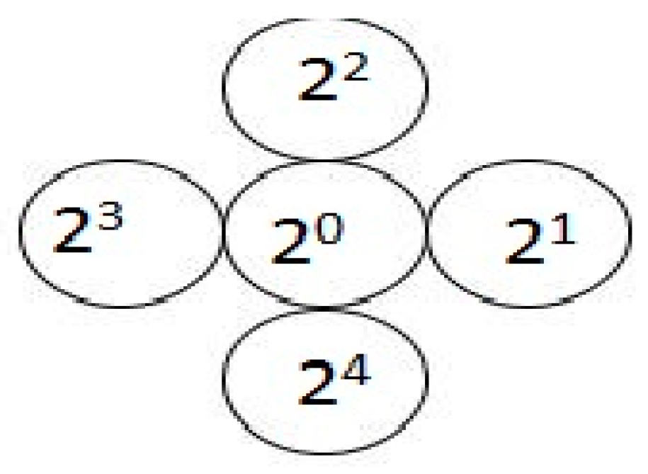
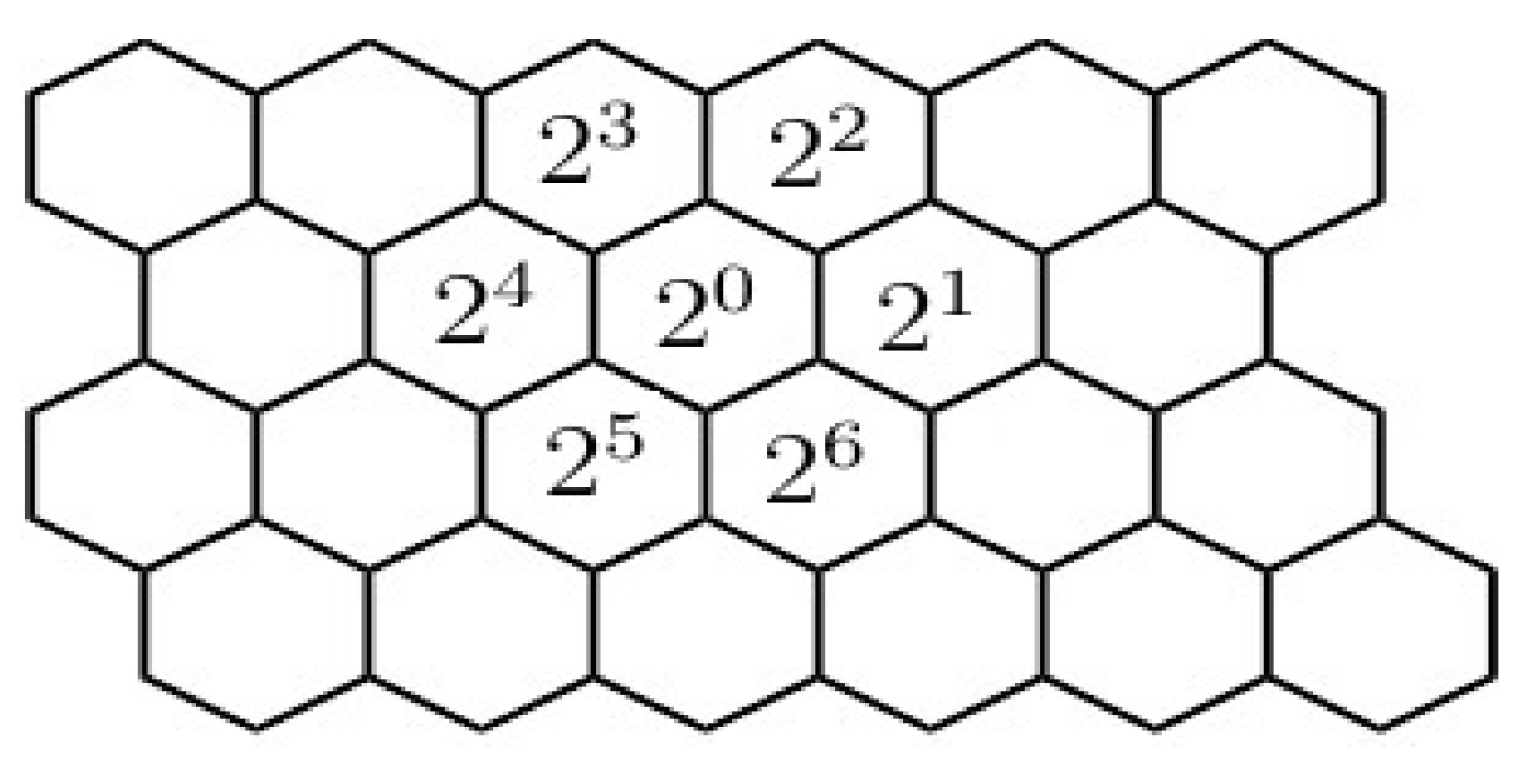
For example, for a circular lattice shown in Figure 5, five neighborhood structures are used. nSG-CA rule $14$ refers to the three neighborhood dependency of the cell $C_{ij}$ to its three neighbors is calculated by the formulae $2^3+2^2+2^1$, where $2^0$ is the positional weight of the cell to be updated ($C_{ij}$). The total number of rules for a two dimensional CA depends on the value of neighborhood, $N_b$. The total number of rules of the nSG-CA model is $2^{N_b}$, which includes the rule characterizing no dependency. For an nSG-CA with a hexagonal lattice has 7 neighborhoods and its positional weight with respect to the cell to be updated ($C_{ij}$) is shown in Figure 6.

In this paper, X-OR is the operation used to update a cell $C_{ij}$ based on its rule number. X-OR is a binary operator and it is commutative.

The total number of rules for different types of two dimensional lattice is different. For a hexagonal lattice, the size of the neighborhood for each cell $C_{ij },$|$N_b$| is 7, so the total rules are 2⁷ = 128, in a square lattice, for each cell $C_{ij}$ with five neighborhood has 32 rules and for each cell $C_{ij}$ in a rectangular lattice with nine neighborhood can generate 512 rules. A variant of hexagonal lattice, where a cell is placed at every 30$°$ w.r.t the cell to be updated has |$N_b$| = 13. So the total number of rules are 2¹³. So in order to find out a rule for a particular application, classification of cellular automata is required.

4. Classification of Two Dimensional Cellular Automata Rules

One principal direction of research in cellular automata is to study the CA dynamics (patterns) which evolves in successive time steps. A detailed analysis of CA dynamics will enable us to understand the emergent behavior of a pattern and the computational capacity of a CA. In other words, CA classification based on the study of its dynamics has been the major focus of researchers. The CA dynamics vary according to the CA rules. To comprehend the behavior of the rules in the proposed model, it is necessary to have a classification based on their properties. Symmetry is a property exists in CA rules. If a CA rule is symmetric its equivalent pattern is also symmetric. Based on this property, classification of CA rules of nSG-CA model for any heterogeneous symmetric lattice is discussed. Since the nSG-CA model is a type of star graph representation of the neighborhood structure, rules are characterized by the neighborhood, each rule in an nSG-CA can also be represented as a star graph. In order to distinguish the neighborhood structure and rule, the star graph representation of a rule is denoted as r-star graph, where r denote rule.

Definition 7 (r-star graph).

It is a subgraph of n-star graph, in which all the vertices and edges are the subsets of nSG-CA.

In order to measure the symmetry in a star graph, graph automorphism [26] can be used.

Definition 8 (Isomorphic graph).

Two graphs$G_1$and$G_2$are isomorphic graphs if$\exists$structure preserving vertex bijection$f: V\left(G_1\right)\to V\left(G_2\right)$.

Definition 9 (Vertex bijection in a graph).

A vertex bijection$f: V\left(G_1\right)\to V\left(G_2\right)$between two graphs$G_1$and$G_2$if, the total number of edges between every pair of vertices$V_i$and$V_j$in graph$G_1$is equal to the total number of edges between their images$f(V_i)$and$f(V_j$) in graph G₂. A vertex bijection$f: V\left(G_1\right)\to V\left(G_2\right)$is structure preserving if$V_i$and$V_j$are adjacent in$G_1$⇔$f(V_i)$and$f(V_j)$are adjacent in$G_2$.

Definition 10 (Graph automorphism).

An automorphism of a graph G is the isomorphism [26] with itself, i.e., $\exists$ structure preserving vertex bijection $f: V\left(G\right)\to V\left(G\right)$.

The set of automorphisms defines a permutation group known as the automorphisms group. A permutation $\gamma$ of $V\left(G\right)$ is an automorphism of $G$ if for all $V_i$, $V_j$ $ϵ V \left(G\right)$ then, $\left\{\left(V_i, V_j\right)\right\} ϵ E\left(G\right)\iff \left\{\gamma \left(V_i\right), \gamma \left(V_j\right)\right\} ϵ E\left(G\right)$. The set of automorphisms of a graph $G$ under the operation, composition of functions, forms a subgroup of the symmetric group of $V\left(G\right)$ called the automorphism group [26,27] of G. For example, the total number of automorphism for a star graph ($S_N$) is $N!$. In Ref. [28], graph automorphism is used to find the symmetries in a cellular automata, where the global dynamics of a CA are viewed as a graph. So, the concept of graph automorphism can be used as a transformation in an r-star graph to measure the symmetry in a rule.

4.1. CA Rules Based on Symmetry

The r-star graph representation of rule 62 in a rectangular lattice with nine neighborhood nSG-CA is shown in Figure 7. In rule 62, the cell $C_{ij}$ depends on five neighborhood cells among nine neighborhoods for its updation. The dependant cells of $C_{ij}$ are marked using bold line and the nondependant cells are marked using a dotted line in the r-star graph representation of rule 62.

4.1.1.Representation of a given rule

A rule $f$ can be represented as

$$f={{\displaystyle \sum }}_{l=0}^{N-1} a\ast 2^l$$

(2)

where $a$ is coefficient and $a ϵ \left\{0, 1\right\}$, $\ast$ is the multiplication operator.

For example, Rule 25 in a rectangular lattice with five neighborhoods can be represented as shown in Figure 8.

$$\left(1\ast 2^4\right)+\left(1\ast 2^3\right)+\left(0\ast 2^2\right)+\left(0\ast 2^1\right)+\left(1\ast 2^0\right)=25$$

Automorphisms of a graph is a permutation of its vertex set that preserves incidences of vertices and edges. Since automorphism of a graph is a structure preserving vertex bijection, a transformation is required for the possible mapping of vertices in the r-star graph. So a transformation called $\Theta$-transformation is defined as follows.

Definition 11 ($\Theta$-transformation).

Let$f={\alpha }_{0}C\left(0,0\right)\oplus {\alpha }_{1}C\left(1, 0\ast \theta \right)\oplus {\alpha }_{2}C\left(1, 1\ast \theta \right)\oplus ,\dots ,\oplus {\alpha }_{N}C\left(1, \left(N-1\right)\ast \theta \right)$be a rule in nSG-CA, where${\alpha }_i ϵ\left\{0,1\right\}\forall i ϵ\left\{0,\dots ,N\right\}$, let$\mathit{\Theta }=\left(0,l_0\theta ,l_1\theta ,\dots ,l_{N-1}\theta \right)$be a transform on the rule$f$, where$l_0, l_1, l_2 ,\dots ,l_{N-1} ϵ \left\{0, 1,\dots ,N-1\right\}$.

The $\Theta$-transform on $f$ is defined as,

$$f^{*}=f\Theta ={\mathsf{\alpha }}_{0}C\left(0,0\right)\oplus {\mathsf{\alpha }}_{1}C\left(1,(0\theta +l_1\theta \right)\mathrm{Mod}\mathrm{N}\theta )\oplus {\mathsf{\alpha }}_{2}C\left(1,(1\theta +l_2\theta \right)\mathrm{Mod}\mathrm{N}\theta ),\dots .,{\mathsf{\alpha }}_{N}C\left(1,(\left(N-1\right)\theta +l_{N-1}\theta \right)\mathrm{Mod}\mathrm{N}\theta )$$

The set of all $\Theta$-transformations of the rule $f$ are the set of automorphisms of the r-star graph; that is $N!$. It is equivalent to the total automorphisms of the star graph.

Definition 12 (Symmetric rule).

A rule$f$is said to be symmetric rule, if ∃ a bijective$\mathit{\Theta }$transformation such that$f\mathit{\Theta }=f$.

One of the major focus of this work is to find out the symmetric rules (local internal symmetry), which generate symmetric patterns w.r.t. the line $\theta =90°$. The following theorem supports to define the symmetry in rules w.r.t vertical axis, line $\theta =90°$.

Theorem 1.

In a two state two dimensional nSG-CA, the reflection of the edge$\left(C\left(0, 0\right), C\left(1, l \theta \right)\right)$w.r.t line$\theta =90°$in the r-star graph of any rule$f$is$\left(C\left(0,0\right), C\left(180-l \theta \right)\right)$.

Proof. 

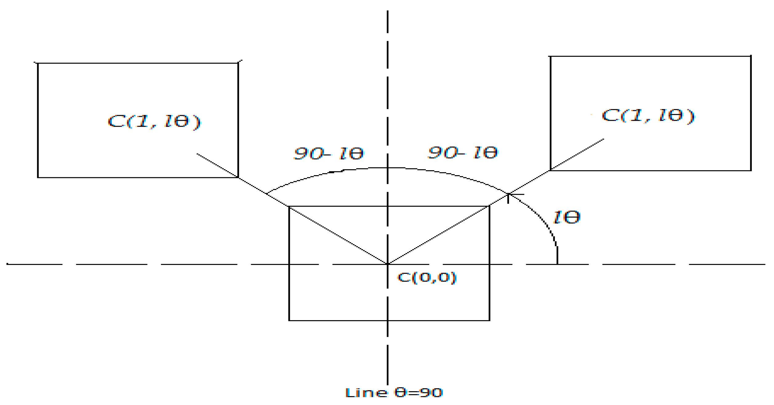
Without loss of any generality, we assume a rectangular lattice for two dimensional nSG-CA. Let $C\left(1,l\theta \right)$ be a cell in the neighborhood of $C\left(0, 0\right)$. By the description of our nSG-CA model, the polar angle($\theta )$, between the edge $\left(C\left(0, 0\right), C\left(1, l \theta \right)\right)$ with the initial line is $l \theta$. Then the angle between the edge $\left(C\left(0, 0\right), C\left(1, l \theta \right)\right)$ with the axis of reflection $\theta =90°$ is $90-l\theta$. In a reflection of a line w.r.t an axis, the axis of reflection should bisect the angle between the original line and the reflected line. The only line which will make an angle $90-l\theta$ with the axis of reflection $\theta =90°$ is the edge of the star graph which will have a polar angle of $l\theta +90-l \theta +90-l \theta$ = $180-l \theta$, as shown in Figure 9, i.e. in our nSG-CA model, edge, $\left(C\left(0,0\right), C\left(180-l \theta \right)\right)$ can have an angle of $180-l\theta$ with the pole. Further, we observe that line $\theta =90°$ is the perpendicular bisector of the angle between the edges ($C\left(0,0\right), C\left(1, l\theta \right))$ and ($C\left(0, 0\right), C\left(1, 180-l\theta \right))$. Hence the reflection of the edge ($C\left(0,0\right), C\left(1, \theta \right))$ w.r.t line $\theta =90°$ is ($C\left(0, 0\right), C\left(1,180-l \theta \right))$. This completes the proof.

Based on the above Theorem 1, the symmetry in rules w.r.t. the line $\theta =90°$, which is denoted as self symmetry is defined.

Definition 13 (Self-symmetry in a rule).

A rule$f$is said to be self symmetric in the r-star graph, if it satisfies the following conditions:

1. 

$f$is a symmetric rule, where$\mathit{\Theta }=\left(0,l_0\theta ,l_1\theta ,\dots \dots ,l_{N-1}\theta \right)$is a bijective transform of$f$

2. 

$l_i\theta$$ϵ$$\mathit{\Theta }$if and only if$180-l_i\theta ϵ \mathit{\Theta } \forall i ϵ \left\{0,1,\dots N-1\right\}$

Definition 14 (Pairwise symmetric rules).

Let$f={\alpha }_{0}C\left(0,0\right)\oplus {\alpha }_{1}C\left(1,0\theta \right)\oplus {\alpha }_{2}C\left(1,1\theta \right)\oplus \dots \dots \oplus {\alpha }_{N}C\left(1,\left(N-1\right)\theta \right)$be a rule in an r-star graph, where${\alpha }_0, {\alpha }_1,\dots ,{\alpha }_N ϵ\left\{0,1\right\}$. Let a transform${\mathit{\Theta }}^{*}=\left(0, 180-0\theta , 180-1\theta ,\dots ,180-\left(N-1\right)\theta \right)$on the rule$f$. The rules$f{\mathit{\Theta }}^{*}$and$f$are said to be pairwise symmetric rules if$f{\mathit{\Theta }}^{*}\ne f$.

4.2. Algorithm to Identify the Nature of Symmetry in CA Rules

The following algorithm (Algorithm 1) is used to identify the nature of symmetry in CA rules.

Algorithm 1. Identification of type of symmetry in a rule.
Input: Rule number, $f$ or Conclude that $f$  Output: Returns the pairwise symmetric pair rules of f or      Conclude that f is self-symmetric
Initialization	1 Let $2^p$ be a partition of $f$ with coefficient 1 2 Let $L$ be a horizontal line passing through the cell to be updated on $X$-Axis. 3 Initialize variables, $‘s’$, $image$ and $d$ as 0
Iteration for partition checking	4 for each $2^p$ in $f$ 5 case 1: 6 Let $2^i$ and $2^j$ be two partitions coincide with $L$ such that $2^i$ is on the left side and $2^j$ is on the right side w.r.t the cell to be updated. 7 Assign $2^j=2^1$
Partition is in upper half	8  If $(0<\Phi \left(2^p\right)<=180)$ 9   If $\left(2^p equals 2^i\right)$ 10     $image=2^j$ 11     $else if (2^p<2^i)$ 12      $d=i–p$ 13      $image=2^{j+d}$ 14     $end elseIf$ 15$s=s+image$ 16 case 2:
Partition is in the lower half	17 $Let 2^j=2^{N+1}$ where $N=360/\theta$ 18 $If (180<\Phi \left(2^p\right)<=360)$ 19  $If(2^p>2^i)$ 20   $d=p–i$ 21    $image=2^{j-d}$ 22   $end if$ 23  $s=s+image$ 24  case 3: 25  $If\left(2^{p}equals 2^0\right)$ 26  $image=2^0$ 27  $s=s+image$
Partition checking iteration	28  $end for$
Nature of rule	29  $if \left(s equals f\right)$ given rule $f$ is self-symmetric 30 else 31  rules $s and f$ are pairwise symmetric

4.2.1. Description of Algorithm

The algorithm to identify the nature of symmetry for a given rule is shown in Algorithm1. In order to identify the nature of symmetry exists in a rule, the given rule is partitioned into powers of 2 based on the Equation (2). Assuming that a horizontal line L is passed through the cell to be updated and it contains two partitions such as $2^i$ in the left side of cell to be updated and $2^j$ in the right side of the cell to be updated. Each partition of a rule is either at the top or bottom of the line L. Thus, two cases are considered. Case 1 checks whether the partition is in the top of the line L or not and find out the equivalent reflection of each partition. Case 2 checks for the partitions which are in the bottom of the line L and find out its equivalent reflections. Case 3 checks whether the partition includes the cell to be updated or not and find out the reflection. If the sum of the reflections of a rule is same as the given rule number, then conclude that the given rule is self-symmetric and the sum of the reflections of its partitions of the given rule differs from the given rule, then conclude that they are pairwise symmetric rules. The Algorithm 1 takes polynomial time complexity only to check the nature of the rules.

4.2.2. Illustration

Consider a rule 25 in a hexagonal lattice with seven neighborhoods. The partitions of the rule 25 with coefficient 1 are $2^4$, $2^3$, and $2^0$. Consider each of the partitions, $2^p$ as $2^4$, then $2^p$ equals $2^i$ so, the image is $2^1$. The second partition is $2^3$, so consider $2^p$ as $2^3$ which is lesser than $2^p$, then $d=4–3$, i.e., 1. Then the image is $2^{1+1}$ i.e., $2^2$. The third partition is $2^0$, then the image is $2^0$ itself. So the sum of $2^1$, $2^2$, and $2^0$ is 7, which is not equal to 25. So conclude that rule 7 and rule 25 are pairwise symmetric rules in a hexagonal lattice with seven neighborhoods.

4.3. Global Symmetry (Symmetry in Pattern)

The local internal symmetry of the rule $f$ is discussed in the session 4.2. The connection between local internal symmetries and the dynamics of nSG-CA is provided by global symmetries, which are obtained as concatenations of local internal symmetries. Figure 10 shows the r-star graph of a self-symmetric rule, in the figure 10, the edges present in the r-star graph is marked as bold. If the rule is self symmetric, the cell state set of the rule is partitioned into three disjoint sets w.r.t. the vertical line. They are as follows:

(a)

State set in the left side of the vertical line;

(b)

State set on the right side of the vertical line;

(c)

State set is on the vertical line.

To illustrate this, let us consider a rule $f$,

$$f=C\left(0,0\right)\oplus \mathrm{C}\left(1,45°\right)\oplus \mathrm{C}\left(1,135°\right)\oplus \mathrm{C}\left(1,225°\right)\oplus \mathrm{C}\left(1,315°\right),\Theta =\left(0, 90°,270°,90°,270°\right)$$

is a transform of the rule $f,$ since $f\Theta =f$ and $f$ is a symmetric rule, $\left\{\mathrm{C}\left(1,135°\right), \mathrm{C}\left(1,45°\right)\right\},\left\{\mathrm{C}\left(1,225°\right), \mathrm{C}\left(1,315°\right)\right\}$ are local internal symmetries of the rule $f$ as shown in the Figure 10. The cell state set of $f$ is $A=\left\{C\left(0,0\right), \mathrm{C}\left(1,45°\right),\mathrm{C}\left(1,135°\right),\mathrm{C}\left(1,225°\right),\mathrm{C}\left(1,315°\right)\right\}$ can be divided into three sets. They are,

• $A_1=\left\{\mathrm{C}\left(1,135°\right),\mathrm{C}\left(1,225°\right)\right\}$ is on the left side of the vertical line
• $A_2=\left\{\mathrm{C}\left(1,45°\right),\mathrm{C}\left(1,315°\right)\right\}$ is in the right side of the vertical line
• $A_3=\left\{C\left(0,0\right)\right\}$ is the cell on the vertical line.

nSG-CA is a dynamical system $({(Z_K)}^z$ x, $\left(Z_K{)}^z,f\right)$ where evolution is the state space ${(Z_K)}^z$ x, ${(Z_K)}^z$ is obtained in discrete steps by the repeated iteration of the global evolution rule.

$F:{(Z_K)}^z$ x, ${(Z_K)}^z$ → ${(Z_K)}^z$ x, ${(Z_K)}^z$, where $K=\left\{0,1\right\}$. The global evolution rule $F$ is induced by a local rule $f: {(Z_K)}^{2r+1}$ x, ${(Z_K)}^{2r+1}\to Z_K$, $2r$ is the number of neighbors of the central cell. If $f$ is self symmetric, then the rule set can be partitioned into three disjoint sets. Let $A_1$ is the cells of the left side, $A_2$ is the cells on the right side of the vertical line, $\theta =90°$, and $A_3$ is on the vertical line. For the input configuration $x$, the evolving state set of $A_1$ and the evolving state of $A_2$ are symmetric, because of the internal symmetry of each cell. The evolving state set of $A_3$ are also symmetric since, cells of $A_3$ are on the vertical line. Therefore, the self-symmetric rule $f$ generates symmetric pattern $F$, which is symmetric w.r.t. line $\theta =90°$ obtained by $A_1$, $A_2$ and $A_3$ act on an input configuration $x$.

5. Results

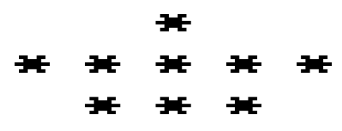
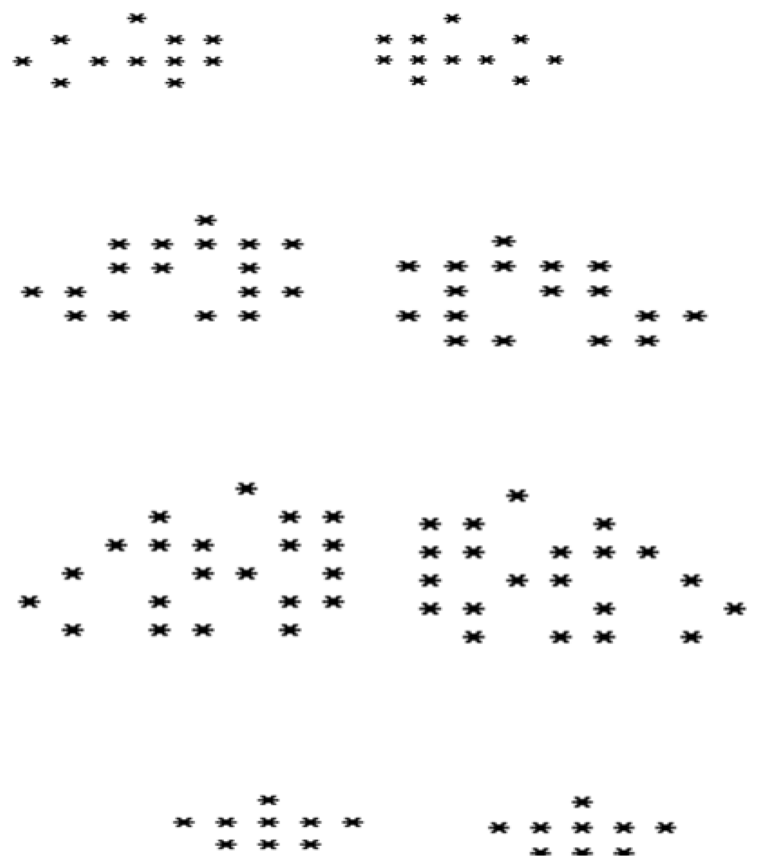
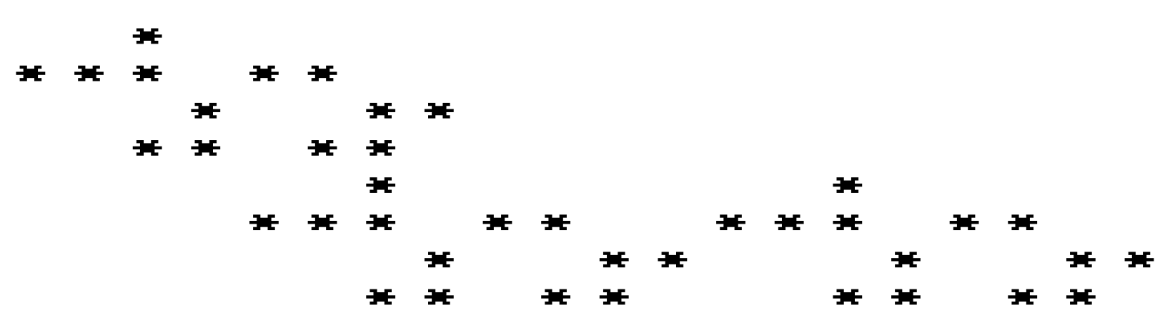
There are two types of symmetric rules with respect to line $\theta =90°$ in an nSG-CA model. They are pairwise symmetric rules and self-symmetric rules. The nSG-CA model is based on null boundary conditions. X-OR is considered as the operator for the experiments. Consider a rectangular lattice with five neighborhood cells. Figure 11 shows the initial seed image, where $\ast$ represents 1 and space represents 0. In order to generate a pattern, X-OR operation is applied to all the cells in the neighborhood with the cell to be updated. The uniform rule is applied to all the cells w.r.t the cell to be updated at each time step in parallel. Null boundary conditions are applied. The symmetry axis is a vertical line passing through 90$°$. Figure 12 shows the pattern of rule 19 and rule 25 in a rectangular lattice with five neighborhood structure. The evolving pattern in four iterations are shown in the Figure 12. From the figure, it is observed that both the patterns are pairwise symmetric. i.e., symmetric with respect to axis, $\theta =90°$. Figure 13 shows the pattern of the rule 31 in a rectangular lattice with five neighborhoods at 8th iteration, which shows a self-symmetric pattern.

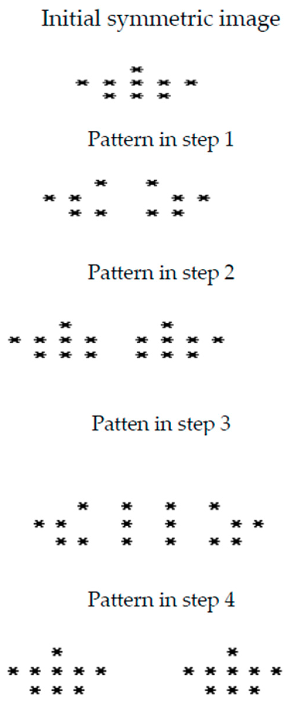
In order to understand the behavior of the X-OR rule, an evolution of X-OR for four iterations on a symmetric initial seed is shown in Figure 14. From this, one can observe that if the input is symmetric and if we apply a symmetric rule it generates a symmetric pattern at every time step.

The classification of symmetric rules in a rectangular lattice with five neighborhood is shown in

Table 1. Classification of rules in a rectangular CA lattice with N = 5, where PR denotes pairwise symmetric rules and self-denotes self-symmetric rules.

5C1		5C2		5C3		5C4		5C5
PR	Self	PR	Self	PR	Self	PR	Self	PR	Self
$R \left(2,8\right)$	$R\left(1\right)$	$R\left(12,6\right)$	$R\left(5\right)$	$R\left(7,13\right)$	$R\left(11\right)$	$R\left(23,29\right)$	$R(15$)	-	$R\left(31\right)$
$R\left(4,16\right)$		$R(3,9$)	$R(10$)	$R\left(25,19\right)$	$R\left(14\right)$		$R\left(27\right)$	-
		$R\left(24,18\right)$	$R(17$)	$R\left(22,28\right)$	$R\left(21\right)$		$R\left(30\right)$	-
			$R\left(20\right)$		$R\left(26\right)$			-

. The total 31 rules are classified into five classes based on the number of cells dependent on the cells to be updated among the five neighborhood cells. Thus ⁵C₁ indicates dependency of one neighborhood to the cell to be updated among five neighborhoods; ⁵C₂, ⁵C₃, ⁵C₄, ⁵C₅ indicates the dependency of two, three, four, and five neighborhood cells to the cell to be updated, respectively.

Consider a hexagonal lattice with seven neighborhoods and an initial seed image shown in Figure 11. Then, Figure 15 and Figure 16 indicate two pair rules which are generating pairwise symmetric patters. Figure 16 indicates the pattern of rule 28 in a hexagonal lattice for six iterations. The Pattern generated for Rule 14 in a hexagonal lattice for six iterations is shown in Figure 16. Self-symmetric pattern of rule 97 for eight iterations is shown in Figure 17.

The classification of symmetric rules in a hexagonal lattice with seven neighborhood cells are shown in

Table 2. Classification of rules in a hexagonal lattice with seven neighboring cells.

7C1		7C2		7C3		7C4		7C5		7C6		7C7
PR	Self	PR	Self	PR	Self	PR	Self	PR	Self	PR	Self	Self
(8,4)	1	(17,3)	12	(25,7)	13	(92,46)	30	(93,47)	31	(123,119)	126	127
(16,2)		(9,5)	96	(21,11)	97	(60,78)	114	(61,79)	109	(125,111)
(32,64)		(33,65)	18	(81,35)	19	(102,120)	108	(103,121)	115	(63,95)
		(24,6)		(49,67)		(86,58)		(87,59)
		(48,66)		(37,73)		(106,116)		(107,117)
		(20,10)		(69,41)		(54,90)		(55,91)
		(80,34)		(28,14)		(105,101)		(62,94)
		(72,36)		(88,38)		(71,57)		(118,122)
		(68,40)		(56,70)		(39,89)		(124,110)
				(84,42)		(99,113)
				(52,74)		(29,15)
				(82,50)		(27,23)
				(112,98)		(85,43)
				(74,44)		(53,75)
				(104,100)		(83,51)
				(22,26)		(77,45)

. There are 128 rules in a two dimensional CA with hexagonal lattice including rule 0. These rules are classified into seven classes based on the number of cells dependent on the cells to be updated among the seven neighborhood cells. Thus ⁷C₁ indicates dependency of one neighborhood to the cell to be updated among seven neighborhoods cells; ⁷C₂, ⁷C₃, ⁷C₄, ⁷C₅, ⁷C₆, ⁷C₇ indicates the dependency of two, three, four, five, six, and seven neighborhood cells to the cell to be updated respectively. PR denote pairwise symmetric rules, which are mentioned in brackets and self-denote the self-symmetric rules in a two dimensional CA with hexagonal lattice. There are no pairwise symmetric rules in ⁷C₇ category.

6. Discussion

In order to simulate various complex systems, where the underlying lattices may be different in nature using cellular automata, the angle based model is used. nSG-CA model can be used to accommodate various types of neighborhood structures with the angle($\theta$) concept. The generic rule convention used in nSG-CA generates unique rules for each symmetric lattice. Every rule in an nSG-CA model with a specific lattice gets a unique number i.e., no two rules have the same number in a lattice.

The algorithm proposed in this paper can be used to check the symmetric nature of each rule in a specific lattice. In order to measure the symmetry in a rule, which is represented as r-star graph, a $\Theta$-transform based on graph automorphism is used. A rule $f$ is said to be symmetric if $f=f\Theta$.

Self-symmetric rule is defined based on subset of $\Theta$-transform, i.e., a rule is self-symmetric w.r.t the line $=90°$, if the reflection of all the vertices in the r-star graph w.r.t line $\theta =90°$ is a vertex in the r-star graph if self. The self-symmetric rules generate self-symmetric patterns if the input data are symmetric. A mechanism is discussed in this paper to reflect the self-symmetry exists in a rule to the output pattern (global symmetry). Pairwise symmetric rules are also defined based on ${\Theta }^{*}$-transformation. Two pairwise symmetric rules together generate a bilateral symmetric pattern if the input is symmetric.

The angle concept used in this work is as follows, the polar angle and input angle ($\theta$) are the key parameters of this work. With the input angle$\left(\theta \right)$, we can accommodate any two dimensional symmetric lattices in a CA. A generic rule convention, which suits for any symmetric lattice could derive with relationship between the polar angle and input angle $\left(\theta \right)$ of cells in a two dimensional CA. In order to find the symmetry in rules, $\Theta$-transform is used based on the angle. So, with one parameter, all the concepts discussed in this work are covered.

6.1. Applications of the Proposed nSG-CA Model

Symmetry is a property observed in many objects in our day to day life, such as architectures, arts, natural objects, human body, etc. has a lot of applications in our day to day life [29]. Bilateral symmetry i.e., vertical symmetry computation of shapes and images is a basic problem in computer vision, image processing, and mathematics. The work, such as the use of bilateral symmetry in facial recognition [30,31], 3D face authentication, and recognition based on bilateral symmetry analysis [32,33], bilateral symmetry in modeling the human body to recognize an automated person [34], and in feature restoration to recover features that are invisible [34], has used bilaterally symmetry analysis of the pattern generated from the models; CA is used for image processing [35] applications.

The main application of the nSG-CA model is to find out the asymmetry in symmetric images such as brain anomaly detection, anomaly detection in mammograms, etc. The brain exhibits a high level of bilateral symmetry and it gets violated in the presence of an anomaly. So with the pairwise symmetric rules, one can find out the anomaly in brain images. Similarly like any other objects which exhibits symmetry with respect to line $\theta =90°$.

Since CA is used for modeling complex systems [36], the nSG-CA model is suitable for modeling different types of symmetric regular lattices such as the square lattice, rectangular lattice, hexagonal lattice, etc. In crashworthy applications, in order to absorb more crash energy, different variants hexagonal lattice such as honeycomb structures [37,38] where cells are placed in $60°,30°,15°,$ etc. are used. Since cellular automata can be used as a platform to simulate crash worthy applications [39], using the nSG-CA model, one can simulate any applications with honeycomb structures because, the representation of honeycomb structure is easy with this proposed model. Moreover, all the rules of the proposed model are bilaterally symmetric. Since the symmetric rules are capable of generating symmetric patterns, using this nSG-CA model, one can generate symmetric patterns based on various types of lattice to model various complex systems.

6.2. Comparison with Existing Models

The existing two dimensional CA models such as the Moore neighborhood [1] and von Neumann neighborhood [8] are used for the representation of rectangular lattices with nine neighborhoods and five neighborhoods. Other fixed weight neighborhood models [10] and the seven neighborhood hexagonal model [12], which is based on the fixed weight neighborhood model, also exist. Instead of multiple models, one can represent any symmetric lattice such as a rectangular lattice, hexagonal lattice, circular lattice, square lattice, etc. using the nSG-CA model based on an angle itself.

In many of the applications, in order to generate bilateral symmetric patterns i.e., vertical symmetric patterns, pairwise symmetrical CA rules are required. The classification of symmetric rules discussed in [14,15,16] requires exponential time complexity to identify a pairwise symmetric rules which can generate a bilateral symmetric pattern, because they are defined based on a permutation approach. However in this work an algorithm is proposed to find the self-symmetric rule and a pairwise symmetric rule in polynomial time, which generates bilateral symmetric patterns.

7. Conclusions

This paper has described a cellular automata model with which one can model any uniform CA with various types of regular lattices such as rectangular lattice, circular lattice, hexagonal lattice etc. where each cell is surrounded by an even number of cells. A mathematical formula is proposed to generate rules in a 2D-CA based on various types of underlying lattice. A polynomial time algorithm is proposed to identify self-symmetric rules and pairwise symmetric rules in any type of symmetric lattice in a two dimensional CA, which are capable of generating symmetric patterns. This paper focused on the symmetry w.r.t the middle of the lattice. The scope of this paper can be extended to study any type of symmetry with reference to any axis. The results of this paper can be applied to anomaly detection in symmetric objects that exists in nature, leading to many vital applications such as brain tumor, facial anomaly etc.

References

- Wolfram, S. Statistical mechanics of cellular automata. Rev. Mod. Phys. 1983, 55, 601. [Google Scholar] [CrossRef]
- Brockfeld, E.; Barlovic, R.; Schadschneider, A.; Schreckenberg, M. Optimizing traffic lights in a cellular automaton model for city traffic. Phys. Rev. E 2001, 64, 056132. [Google Scholar] [CrossRef] [PubMed]
- Mozumder, C.K. Topometry Optimization of Sheet Metal Structures for Crashworthiness Design Using Hybrid Cellular Automata; University of Notre Dame: Notre Dame, IN, USA, 2010. [Google Scholar]
- Arredo, J.I.; Kasanko, M.; McCormick, N.; Lavalle, C. Modelling dynamic spatial processes: Simulation of urban future scenarios through cellular automata. Landsc. Urban Plan. 2003, 64, 145–160. [Google Scholar] [CrossRef]
- Batty, M.; Xie, Y.; Sun, Z. Modeling urban dynamics through GIS-based cellular automata. Comput. Environ. Urban Syst. 1999, 23, 205–233. [Google Scholar] [CrossRef] [Green Version]
- Małecki, K. Two-Way Road Cellular Automaton Model with Loading/Unloading Bays for Traffic Flow Simulation. In Proceedings of the 13th International Conference on Cellular Automata for Research and Industry, ACRI 2018, Como, Italy, 17–21 September 2018; pp. 218–229. [Google Scholar]
- Packard, N.H.; Wolfram, S. Two-dimensional cellular automata. J. Stat. Phys. 1985, 38, 901–946. [Google Scholar] [CrossRef]
- Von Neumann, J.; Burks, A.W. Theory of Self-Reproducing Automata; University of Illinois: Urbana, IL, USA, 1996; p. 8. [Google Scholar]
- Toffoli, T.; Margolus, N. Cellular Automata Machines: A New Environment for Modeling; MIT Press: Cambridge, MA, USA, 1987. [Google Scholar]
- Khan, A.R.; Choudhury, P.P.; Dihidar, K.; Mitra, S.; Sarkar, P. VLSI architecture of a cellular automata Machine. Comput. Math. Appl. 1997, 33, 79–94. [Google Scholar] [CrossRef]
- Kornyak, V.V. Cellular automata with symmetric local rules. In International Workshop on Computer Algebra in Scientific Computing; Springer: Berlin/Heidelberg, Germany, 2006; pp. 240–250. [Google Scholar]
- Mohammed, J.; Sahoo, S. Design and Analysis of Matrices for Two Dimensional Cellular Automata Linear rules in Hexagonal Neighborhood. Math. Atern. 2011, 1, 537–545. [Google Scholar]
- Uguz, S.; Ugur, S.; Ferat, S. Uniform cellular automata linear rules for edge detection. In Proceedings of the 2013 IEEE International Conference on Systems, Man, and Cybernetics, Manchester, UK, 13–16 October 2013; pp. 2945–2950. [Google Scholar]
- Choudhury, P.P.; Sahoo, S.; Hasssan, S.; Basu, S.; Ghosh, S.; Kar, D. Classification of cellular automata rules based on their properties. arXiv, 2009; arXiv:0905.1769. [Google Scholar]
- Khan, A.R. Classification of 2D cellular automata uniform group rules. Eur. J. Sci. Res. 2011, 64, 51–57. [Google Scholar]
- Kazlacheva, Z. Symmetry in Nature and Symmetry in Fashion Design. Econ. Manag. Inf. Technol. EMIT 2013, 1, 267. [Google Scholar]
- Nakashima, M.; Reddi, A.H. The application of bone morphogenetic proteins to dental tissue engineering. Nat. Biotechnol. 2003, 21, 1025. [Google Scholar] [CrossRef] [PubMed]
- Mardia, K.V.; Bookstein, F.L.; Moreton, I.J. Statistical assessment of bilateral symmetry of shapes. Biometrika 2000, 87, 285–300. [Google Scholar] [CrossRef]
- Mara, D.; Owens, R. Measuring bilateral symmetry in digital images. In Proceedings of the Digital Processing Applications (TENCON ′96), Perth, Australia, 29–29 November 1996; pp. 151–156. [Google Scholar]
- Shi, P.; Zheng, X.; Ratkowsky, D.A.; Li, Y.; Wang, P.; Cheng, L. A Simple Method for Measuring the Bilateral Symmetry of Leaves. Symmetry 2018, 10, 118. [Google Scholar] [CrossRef]
- Enciso, A. Symmetry in Cellular Automata. Electromagn. Phenom. 2006, 6, 17. [Google Scholar]
- García-Morales, V. Symmetry analysis of cellular automata. Phys. Lett. A 2013, 377, 276–285. [Google Scholar] [CrossRef]
- Tanaka, I. Effects of initial symmetry on the global symmetry of one-dimensional legal cellular automata. Symmetry 2015, 7, 1768–1779. [Google Scholar] [CrossRef]
- Salazar, G.; Jesús, U. Internal symmetries of cellular automata via their polynomial representation. Chaos An Interdiscip. J. Nonlinear Sci. 1998, 8, 711–716. [Google Scholar] [CrossRef]
- Yamasaki, K.; Nanjo, K.Z.; Chiba, S. Symmetry and entropy of one-dimensional legal cellular automata. Complex Syst. 2012, 20, 351. [Google Scholar]
- Herstein, I.N. Topics in Algebra; John Wiley & Sons: Hoboken, NJ, USA, 2006. [Google Scholar]
- Golumbic, M.C. Algorithmic Graph Theory and Perfect Graphs; Elsevier: Amsterdam, The Netherlands, 2008; p. 57. [Google Scholar]
- Powley, E.J.; Stepney, S. Automorphisms of Transition Graphs for Elementary Cellular Automata. J. Cell. Autom. 2009, 4, 125–136. [Google Scholar]
- Field, M.; Golubitsky, M. Symmetry in Chaos: A Search for Pattern in Mathematics, Art, and Nature; SIAM: Philadelphia, PA, USA, 2009; p. 111. [Google Scholar]
- Troje, N.F.; Bülthoff, H.H. How is bilateral symmetry of human faces used for recognition of novel views? Vis. Res. 1998, 38, 79–89. [Google Scholar] [CrossRef]
- Zhang, L.; Razdan, A.; Farin, G.; Femiani, J.; Bae, M.; Lockwood, C. 3D face authentication and recognition based on bilateral symmetry analysis. Vis. Comput. 2006, 22, 43–55. [Google Scholar] [CrossRef]
- Yam, C.; Nixon, M.S.; Carter, J.N. Automated person recognition by walking and running via model-based approaches. Pattern Recognit. 2004, 37, 1057–1070. [Google Scholar] [CrossRef]
- Zhao, W. Face recognition: A literature survey. ACM Comput. Surv. (CSUR) 2003, 35, 399–458. [Google Scholar] [CrossRef]
- Tyler, C.W. Human Symmetry Perception and Its Computational Analysis; Psychology Press: Santa Rosa, CA, USA, 2003. [Google Scholar]
- Popovici, A.; Popovici, D. Cellular automata in image processing. In Proceedings of the Fifteenth International Symposium on Mathematical Theory of Networks and Systems, Notre Dame, Indiana, 12 August 2002; Volume 1, pp. 1–6. [Google Scholar]
- Małecki, K. Graph cellular automata with relation-based neighborhoods of cells for complex systems modelling: A case of traffic simulation. Symmetry 2017, 9, 322. [Google Scholar] [CrossRef]
- Schultz, J.; Griese, D.; Ju, J.; Shankar, P.; Summers, J.D.; Thompson, L. Design of honeycomb mesostructures for crushing energy absorption. J. Mech. Des. 2012, 134, 071004. [Google Scholar] [CrossRef]
- Pankaj, P.A. Honeycomb safety structure: Design, analysis and applications in safe road transport. Int. J. Sci. Res. 2018, 7, 133–141. [Google Scholar]
- Guo, L.; Tovar, A.; Penninger, C.L.; Renaud, J.E. Strain-based topology optimisation for crashworthiness using hybrid cellular automata. Int. J. Crashworth. 2011, 16, 239–252. [Google Scholar] [CrossRef]
Figure 1.
Fixed positional weight neighborhood model.
Figure 2.
Angle-based addressing of a cell in a rectangular lattice.
Figure 3.
Graph G.
Figure 4.
n-star graph CA(nSG-CA) neighborhood model of a rectangular lattice with nine neighborhood cells.
Figure 5.
Circular lattice with .
Figure 6.
Hexagonal lattice with .
Figure 7.
r-star graph representation of rule 62 in rectangular lattice with nine neighborhood nSG-CA.
Figure 8.
r-star graph representation of rule 25 in five neighborhood nSG-CA.
Figure 9.
Reflection in the r-star graph.
Figure 10.
r-star graph of a self-symmetric rule.
Figure 11.
Initial seed image.
Figure 12.
Pattern evolution of of rule 19 and rule 25 in a five neighborhood rectangular lattice.
Figure 13.
Self-symmetric pattern of rule 31 with five neighborhoods at 9th iteration in a rectangular lattice.
Figure 14.
Evolution of an X-OR operation of rule 10 in a rectangular axis-5 neighborhood CA based on an initial seed in four steps.
Figure 15.
Rule 28 in a hexagonal lattice at 5th-iteration.
Figure 16.
Rule 14 in a hexagonal lattice at 5th iteration.
Figure 17.
Self-symmetric pattern of rule 97 at 7th iteration in a hexagonal lattice.