Some Applications of the (G′/G,1/G)-Expansion Method for Finding Exact Traveling Wave Solutions of Nonlinear Fractional Evolution Equations

Abstract

In this paper, the $(G^{\prime }/G,1/G)$-expansion method is applied to acquire some new, exact solutions of certain interesting, nonlinear, fractional-order partial differential equations arising in mathematical physics. The considered equations comprise the time-fractional, (2+1)-dimensional extended quantum Zakharov-Kuznetsov equation, and the space-time-fractional generalized Hirota-Satsuma coupled Korteweg-de Vries (KdV) system in the sense of the conformable fractional derivative. Applying traveling wave transformations to the equations, we obtain the corresponding ordinary differential equations in which each of them provides a system of nonlinear algebraic equations when the method is used. As a result, many analytical exact solutions obtained of these equations are expressed in terms of hyperbolic function solutions, trigonometric function solutions, and rational function solutions. The graphical representations of some obtained solutions are demonstrated to better understand their physical features, including bell-shaped solitary wave solutions, singular soliton solutions, solitary wave solutions of kink type, and so on. The method is very efficient, powerful, and reliable for solving the proposed equations and other nonlinear fractional partial differential equations with the aid of a symbolic software package.

1. Introduction

Nonlinear evolution equations (NLEEs), which can be described using partial differential equations (PDEs), play a significant role for understanding qualitative behaviors of many real-world phenomena. Obtaining exact solutions of a complicated nonlinear evolution system makes it possible to visually comprehend the mechanism of the system considered. Nonlinear wave phenomena occur in various scientific and engineering fields, such as quantum mechanics [1], fluid mechanics [2], optical fibers [3], chemical physics and geochemistry [4], solid-state physics [5], and biology [6]. With the advanced development of symbolically computational packages, such as Maple or Mathematica, constructing for the exact traveling wave solutions of NLEEs has become one of the important themes of challenging interest in mathematical physics and the applied sciences.

Over the last few decades, many kinds of solutions of NLEEs, including exact solutions, analytical approximate solutions, and numerical solutions, have been successfully obtained using various and efficient methods. Examples of the methods for obtaining analytical approximate solutions of NLEEs are the Adomian decomposition method (ADM) [7,8], the revised variational iteration method (RVIM) [9], the reduced differential transform method [10], and the homotopy perturbation method (HPM) [11,12]. Useful methods for solving NLEEs numerically are those such as the finite element method [13], the finite volume method [14], and the finite-difference predictor–corrector method [15]. Several efficient and reliable methods which have recently been developed to obtain exact explicit solutions for NLEEs are, for instance, the Jacobi elliptic function method [16], the $(G{}^{\prime }/G)$-expansion method and its various modifications [17,18,19,20], the Exp-function method [21], the sub-equation method [22], the first integral method [23], the modified trial equation method [24,25], and the simplest equation method [26].

Recently, fractional differential equations (FDEs) has been able to be used extensively as the generalized type of integer-order differential equations, including ordinary differential equations and partial differential equations. FDEs have attracted the researchers’ attention for modeling real-world phenomena, such as modeling anomalous diffusion using a nonlinear fractional Fokker–Planck equation with fractional velocity derivatives and Langevin dynamics to elucidate the effect of non-local transport in the plasma turbulence [27]. More examples of applications of FDEs for real-world problems can be found in [28,29,30] and the references therein. In general, systems actually may not rely only on the local time but also on the former time in history. Hence, the memory and hereditary properties of materials and processes can be described using the theory of fractional derivatives and integrals [31,32,33]. In consequence, nonlinear fractional evolution equations (NLFEEs) have been widely investigated in many aspects, for example, solving the equations for solutions and establishing conditions for which their solutions are asymptotically stable. The exploration for exact solutions of NLFEEs is currently of high interest in applied mathematics and engineering research [19,34,35]. However, the objective of our work is to use the $(G{}^{\prime }/G,1/G)$-expansion method to construct exact traveling wave solutions of the following two NLFEEs in the sense of the conformable fractional derivative.

1. The time-fractional (2+1)-dimensional extended quantum Zakharov-Kuznetsov equation [36] is written as:

$$\begin{array}{c}\hfill D_t^{\alpha }u+au{u}_x+b(u_{xxx}+u_{yyy})+c(u_{xyy}+u_{yxx})=0,\end{array}$$

(1)

where $D_t^{\alpha }u$ denotes the conformable fractional derivative of u with respect to t of order $\alpha$ and $a,b,c$ are real constants, and the solution $u(x,y,t)$, which is a function of the time variable t and space variables x and y, represents the potential of electrostatic wave in space. Solutions of the equation elucidates the spreading of optical pulse in fiber optics [36]. Some articles involved in finding exact solutions of Equation (1) are as follows. Raza et al., [36] found the exact solutions of Equation (1), consisting of the trigonometric function, Jacobi elliptic sine-cosine functions, and hyperbolic function solutions, using the trial equation method. Conversely, Ali et al., [37] obtained the exact solutions of Equation (1) using the $(G{}^{\prime }/G^2)$-expansion method and the modified Kudryashov method. Their exact solutions include the trigonometric, hyperbolic, and rational solutions.

2. The space-time-fractional generalized Hirota-Satsuma coupled Korteweg de Vries (KdV) system [38] can be expressed as:

$$\begin{array}{c}\hfill \begin{array}{cc}\hfill D_t^{\rho }u& ={\displaystyle \frac{1}{4}}{D}_x^{3\eta }u+3u{D}_x^{\eta }u+3D_x^{\eta }(-v^2+w),\hfill \\ \hfill D_t^{\rho }v& =-{\displaystyle \frac{1}{2}}{D}_x^{3\eta }v-3u{D}_x^{\eta }v,\hfill \\ \hfill D_t^{\rho }w& =-{\displaystyle \frac{1}{2}}{D}_x^{3\eta }w-3u{D}_x^{\eta }w,\hfill \end{array}\end{array}$$

(2)

where $D_t^{\rho }\phi$ and $D_x^{\eta }\phi$ denote the conformable fractional derivative of $\phi$ with respect to t of order $\rho$ and to x of order $\eta$, respectively. The first-order Hirota-Satsuma coupled KdV system [39], which was first proposed by Satsuma and Hirota in 1981 and obtained from the four reductions of Kadomtsev-Petviashvili (KP) hierarchy [40], describes interactions of two long waves with different dispersion relations, while the generalized first-order Hirota-Satsuma coupled KdV system [40] is one of the essential nonlinear equations in applied mathematics and physics. The system emerges as a special case of the Toda lattice equation, which is used to describe the interaction of neighboring particles of equal mass in a lattice formation with a crystal [41]. The interesting applications of the generalized Hirota-Satsuma coupled KdV system are as follows [41,42,43]. Firstly, it can be used to explain generic properties of string dynamics for strings and multi-strings in constant curvature space. Secondly, the system is associated with most types of long waves with weak dispersion, internal, acoustic, and planetary waves in geophysical hydrodynamics. Therefore, finding solutions of Equation (2) is potentially useful to describing the physical behaviors of the applications, as mentioned above. The associated equations of the generalized Hirota-Satsuma coupled KdV system have been solved using different methods as follows. In 2007, Zhang [44] used the direct algebraic method to construct the exact solutions for the first-order generalized Hirota-Satsuma coupled KdV systems. In 2010, Zigao et al., [45] applied the improved F-expansion method to the variable-coefficient first-order generalized Hirota-Satsuma coupled KdV system for obtaining the new exact solutions. In 2017, Khater et al., [46] found the exact traveling wave solutions of the system using the modified simple equation method, while the time-fractional generalized Hirota-Satsuma coupled KdV system was solved using the direct algebraic method by Neirameh [41] in 2015.

The rest of this article is organized as follows. In Section 2, the description of the conformable fractional derivative and its important properties are presented. In Section 3, the main steps of the $(G{}^{\prime }/G,1/G)$-expansion method is provided. The applications of the method for solving the two problems mentioned are given in Section 4. Finally, the conclusions of this paper are discussed in Section 5.

2. Conformable Fractional Derivative and Its Properties

In this section, the definition of the conformable fractional derivative and its important properties are given as follows.

Definition 1.

Given a function $f:[0,\infty )\to \mathbb{R}$, the conformable fractional derivative of f of order α is defined by [47,48]

$$\begin{array}{c}\hfill D_t^{\alpha }f\left(t\right)=\underset{\epsilon \to 0}{lim}{\displaystyle \frac{f(t+\epsilon t^{1-\alpha })-f\left(t\right)}{\epsilon }},\mathit{for}\mathit{all}t>0,0<\alpha \le 1.\end{array}$$

(3)

If the limit in Equation (3) exists, then we say that f is α-conformable differentiable at a point $t>0$.

Theorem 1.

Let $\alpha \in (0,1]$, and $f\left(t\right),g\left(t\right)$ be α-conformable differentiable at a point $t>0$, then

$$\begin{array}{ccc}\hfill D_t^{\alpha }\left(\lambda \right)& =& 0,\mathrm{where}\lambda =\mathrm{constant},\hfill \\ \hfill D_t^{\alpha }\left(t^{\mu }\right)& =& \mu t^{\mu -\alpha },\mathrm{for}\mathrm{all}\mu \in \mathbb{R},\hfill \\ \hfill D_t^{\alpha }(af\left(t\right)+bg\left(t\right))& =& a{D}_t^{\alpha }f\left(t\right)+b{D}_t^{\alpha }g\left(t\right),\mathrm{for}\mathrm{all}a,b\in \mathbb{R},\hfill \\ \hfill D_t^{\alpha }\left(f\left(t\right)g\left(t\right)\right)& =& f\left(t\right)D_t^{\alpha }g\left(t\right)+g\left(t\right)D_t^{\alpha }f\left(t\right),\hfill \\ \hfill D_t^{\alpha }\left({\displaystyle \frac{f\left(t\right)}{g\left(t\right)}}\right)& =& {\displaystyle \frac{g\left(t\right)D_t^{\alpha }f\left(t\right)-f\left(t\right)D_t^{\alpha }g\left(t\right)}{g{\left(t\right)}^2}}.\hfill \end{array}$$

Remark 1.

Conformable fractional derivative of some functions are as follows [47].

(1) 

$D_t^{\alpha }\left(e^{ct}\right)=c{t}^{1-\alpha }{e}^{ct},$$c\in \mathbb{R}$.

(2) 

$D_t^{\alpha }(sinbt)=b{t}^{1-\alpha }cosbt,b\in \mathbb{R}$.

(3) 

$D_t^{\alpha }(cosbt)=-b{t}^{1-\alpha }sinbt,b\in \mathbb{R}$.

(4) 

$D_t^{\alpha }\left(\frac{1}{\alpha }{t}^{\alpha }\right)=1$.

(5) 

$D_t^{\alpha }\left(f\left(t\right)\right)=t^{1-\alpha }{\displaystyle \frac{df\left(t\right)}{dt}}$, provided that $f\left(t\right)$ is differentiable.

The following chain rule is very useful for transforming a partial differential equation into an ordinary differential equation, which is required for the methods in finding exact solutions of the equations.

Theorem 2.

Let $f:(0,\infty )\to \mathbb{R}$ be a function such that f is differentiable and α-conformable differentiable. Also, let g be a differentiable function defined in the range of f. Then,

$$D_t^{\alpha }(f\circ g)\left(t\right)=t^{1-\alpha }{f}^{\prime }\left(g\left(t\right)\right)g^{\prime }\left(t\right),$$

where the prime notation ${(}^{\prime })$ represents the ordinary derivative.

3. Algorithm of the $(\mathit{G}{}^{\prime }/\mathit{G},\mathbf{1}/\mathit{G})$-Expansion Method

In this section, the description of the $(G{}^{\prime }/G,1/G)$-expansion method [19,49,50,51] is concisely provided. Consider a nonlinear fractional evolution partial differential equation in three independent variables, $x,y$, and t, as follows:

$$F(u,D_t^{\alpha }u,D_x^{\beta }u,D_y^{\gamma }u,D_t^{2\alpha }u,D_t^{\alpha }{D}_x^{\beta }u,D_t^{\alpha }{D}_y^{\gamma }u,\dots )=0,0<\alpha ,\beta ,\gamma \le 1,$$

(4)

where $D_t^{\alpha }u$, $D_x^{\beta }u$, and $D_y^{\gamma }u$ are the conformable derivatives of a dependent variable u with respect to independent variables $t,x,$ and y when F is a polynomial of unknown function $u=u(x,y,t)$, and its various partial derivatives are those in which the highest order derivatives and nonlinear terms are involved.

Using the following traveling wave transformation

$$u(x,y,t)=U\left(\xi \right),\xi =\frac{k{x}^{\beta }}{\beta }+\frac{l{y}^{\gamma }}{\gamma }+\frac{c{t}^{\alpha }}{\alpha },$$

(5)

where $k,l,\mathrm{and}c$ are constants to be determined later, then Equation (4) is reduced to an ODE in $U=U\left(\xi \right)$ as

$$P(U,U^{\prime },U^{″},\dots )=0,$$

(6)

where P is a polynomial of $U\left(\xi \right)$ and its various derivatives. The prime notation ${(}^{\prime })$ in the above equation denotes the derivative with respect to $\xi .$

The following necessary concepts are introduced before providing the main steps of the $(G{}^{\prime }/G,1/G)$-expansion method. Consider the following second-order linear ODE:

$$\begin{array}{c}\hfill G^{″}\left(\xi \right)+\lambda G\left(\xi \right)=\mu ,\end{array}$$

(7)

where the prime notation (${}^{\prime }$) denotes the derivative with respect to $\xi$ and where $\lambda ,\mu ,$ are constants. Next, we set

$$\begin{array}{c}\hfill \varphi \left(\xi \right)={\displaystyle \frac{G^{\prime }\left(\xi \right)}{G\left(\xi \right)}}\mathrm{and}\psi \left(\xi \right)={\displaystyle \frac{1}{G\left(\xi \right)}}.\end{array}$$

(8)

Equations (7) and (8) can be transformed into the system of two nonlinear ODEs, as follows:

$$\begin{array}{c}\hfill {\varphi }^{\prime }=-{\varphi }^2+\mu \psi -\lambda ,{\psi }^{\prime }=-\varphi \psi .\end{array}$$

(9)

The solutions of Equation (7) can be classified into the following three cases.

Case 1: If $\lambda <0,$ then the general solution of Equation (7) is written as

$$\begin{array}{c}\hfill G\left(\xi \right)=A_{1}sinh\left(\xi \sqrt{-\lambda }\right)+A_{2}cosh\left(\xi \sqrt{-\lambda }\right)+{\displaystyle \frac{\mu }{\lambda }},\end{array}$$

(10)

and we have

$$\begin{array}{c}\hfill {\psi }^2={\displaystyle \frac{-\lambda }{{\lambda }^2{\sigma }_1+{\mu }^2}}\left({\varphi }^2-2\mu \psi +\lambda \right),\end{array}$$

(11)

where $A_1$ and $A_2$ are arbitrary constants and ${\sigma }_1=A_1^2-A_2^2.$

Case 2: If $\lambda >0,$ then the general solution of Equation (7) can be given as

$$\begin{array}{c}\hfill G\left(\xi \right)=A_{1}sin\left(\xi \sqrt{\lambda }\right)+A_{2}cos\left(\xi \sqrt{\lambda }\right)+{\displaystyle \frac{\mu }{\lambda }},\end{array}$$

(12)

and we have the following relation

$$\begin{array}{c}\hfill {\psi }^2={\displaystyle \frac{\lambda }{{\lambda }^2{\sigma }_2-{\mu }^2}}\left({\varphi }^2-2\mu \psi +\lambda \right),\end{array}$$

(13)

where $A_1$ and $A_2$ are arbitrary constants and ${\sigma }_2=A_1^2+A_2^2.$

Case 3: If $\lambda =0,$ then the general solution of Equation (7) can be provided as

$$\begin{array}{c}\hfill G\left(\xi \right)={\displaystyle \frac{\mu }{2}}{\xi }^2+A_1\xi +A_2,\end{array}$$

(14)

and the corresponding relation is

$$\begin{array}{c}\hfill {\psi }^2={\displaystyle \frac{1}{A_1^2-2\mu A_2}}\left({\varphi }^2-2\mu \psi \right),\end{array}$$

(15)

where $A_1$ and $A_2$ are arbitrary constants.

The main steps of the $(G{}^{\prime }/G,1/G)$-expansion method are described as follows.

Step 1: Suppose that the solution to Equation (6) can be expressed by a polynomial of the two variables $\varphi$ and $\psi$, as follows:

$$\begin{array}{c}\hfill U\left(\xi \right)=a_0+\sum _{j=1}^N{a}_j{\varphi }^j+\sum _{j=1}^N{b}_j{\varphi }^{j-1}\psi ,\end{array}$$

(16)

where $a_0,a_j$ and $b_j(j=1,2,\dots ,N)$ are constants to be determined later with $a_N^2+b_N^2\ne 0$ and where the functions $\varphi =\varphi \left(\xi \right)$ and $\psi =\psi \left(\xi \right)$ are implicitly associated with Equation (7) using the relations in Equation (8).

Step 2: Determine the positive integer N in Equation (16) by inserting Equation (16) into Equation (6), and then using the homogeneous balance between the highest-order derivatives and the nonlinear terms in Equation (6). If the degree of $U\left(\xi \right)$ is Deg$\left[U\right(\xi \left)\right]=N$, then the degree of other terms will be formulated as follows:

$$\begin{array}{c}\hfill \mathrm{Deg}\left[{\displaystyle \frac{d^{q}U\left(\xi \right)}{d{\xi }^q}}\right]=N+q,\mathrm{Deg}\left[{\left(U\left(\xi \right)\right)}^p{\left({\displaystyle \frac{d^{q}U\left(\xi \right)}{d{\xi }^q}}\right)}^s\right]=Np+s(N+q).\end{array}$$

(17)

In particular, if the balance number N of some nonlinear equations is not a positive integer (e.g., a fraction and a negative integer), then the special transformations are applied for $U\left(\xi \right)$ in Equation (6) to have a new equation in terms of the new function $W\left(\xi \right)$ with a positive integer balance number (see details in [51,52]).

Step 3: Substituting the resulting equation of Equation (16) into Equation (6) with the aid of Equations (9) and (11), the function P in Equation (6) can be transformed into a polynomial in $\varphi$ and $\psi$, in which the degree of $\psi$ is not larger than one. Equating each coefficient of the resulting polynomial to zero, we obtain a system of algebraic equations, which can be solved using symbolic computational packages, such as Maple or Mathematica, for the following unknowns: $a_0,a_j,b_j(j=1,2,\dots ,N),k,l,c,\mu ,\lambda (<0),A_1,\mathrm{and}{A}_2$. The resulting traveling wave solutions generated by this step with the transformation in Equation (5) are expressed in terms of hyperbolic functions.

Step 4: In the same manner as Step 3, substituting the resulting equation of Equation (16) into Equation (6) with the aid of Equations (9) and (13) for the case $\lambda >0$, we can obtain the exact solutions of Equation (4) by using the transformation in Equation (5). They are written as trigonometric functions.

Step 5: Similarly to Step 3, substituting the resulting equation of Equation (16) into Equation (6) with the aid of Equations (9) and (15) for the case $\lambda =0$, we can obtain the traveling wave solutions of Equation (4) by using the transformation in Equation (5). The resulting exact solutions are expressed as rational functions.

Remark 2.

The two-variable $(G^{\prime }/G,1/G)$-expansion method reduces to the $(G^{\prime }/G)$-expansion method when $\mu =0$ and $b_j=0$ in Equations (7) and (16), respectively. In consequence, the $(G^{\prime }/G,1/G)$-expansion method is an extension of the $(G^{\prime }/G)$-expansion method. Hence, the strength of the $(G^{\prime }/G,1/G)$-expansion method beyond the $(G^{\prime }/G)$-expansion method is that the solutions obtained using the second method can be drawn from the solutions obtained using the first one. This is the reason why the $(G^{\prime }/G,1/G)$-expansion method is used in our work instead of the $(G^{\prime }/G)$-expansion method.

4. Applications of the $(\mathit{G}{}^{\prime }/\mathit{G},\mathbf{1}/\mathit{G})$-Expansion Method

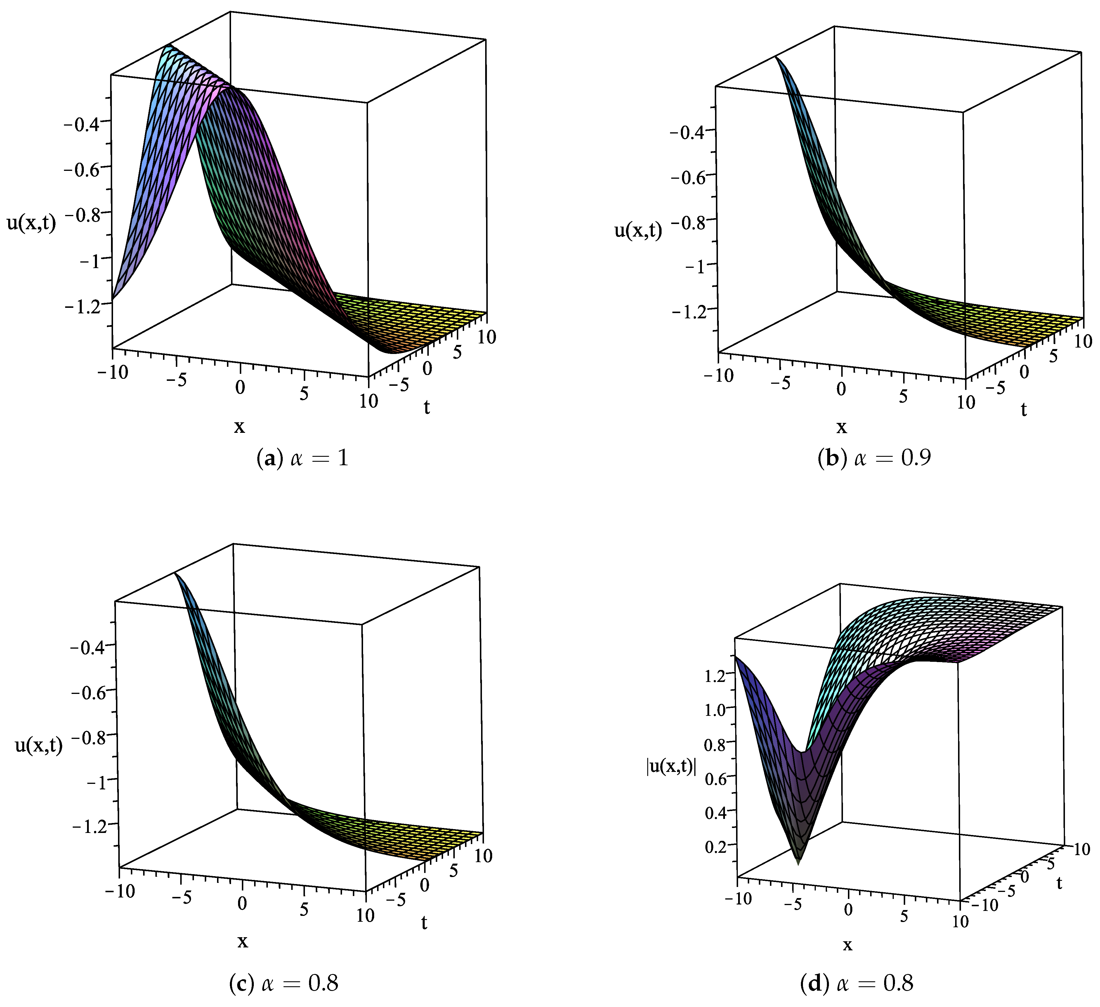
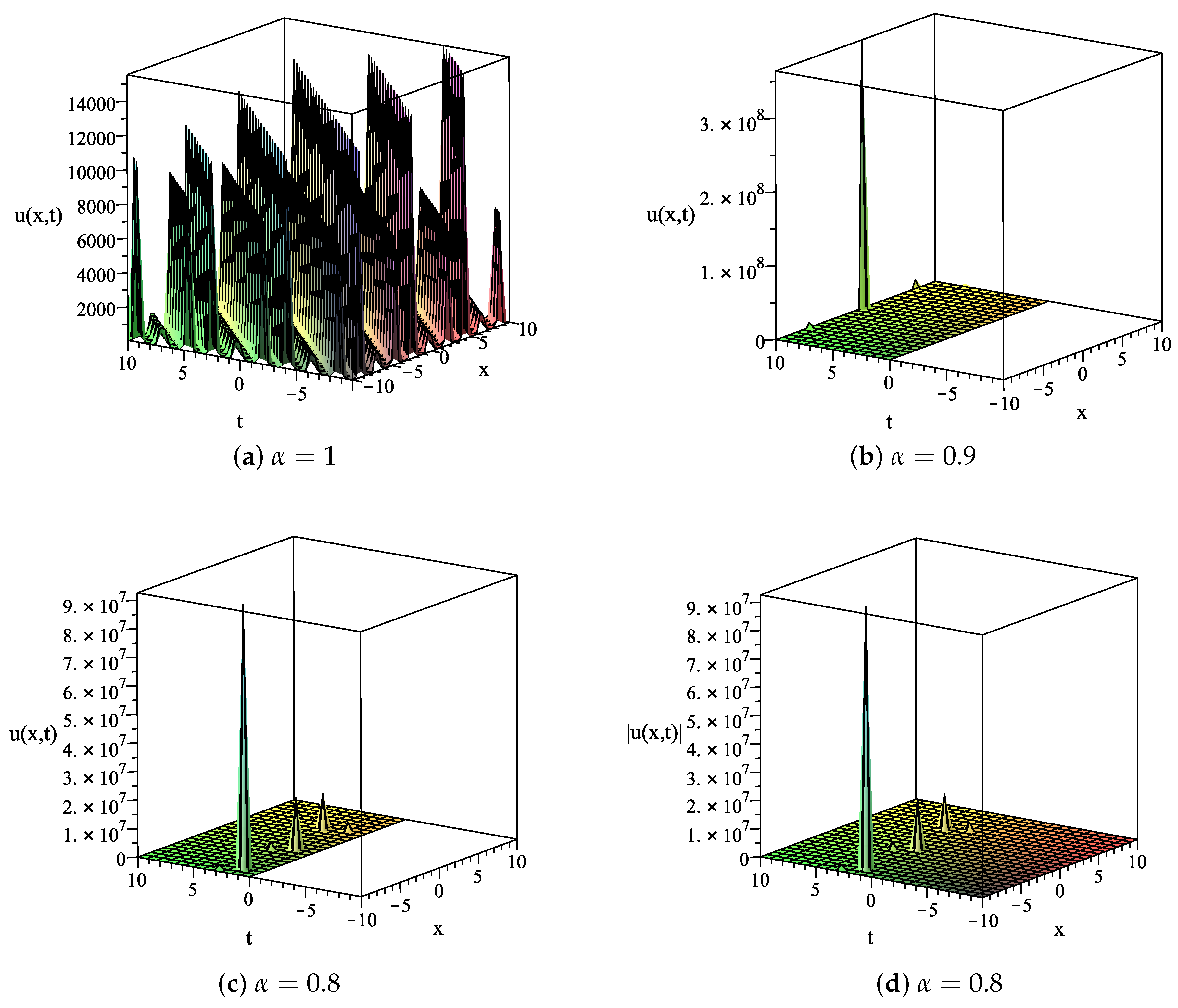
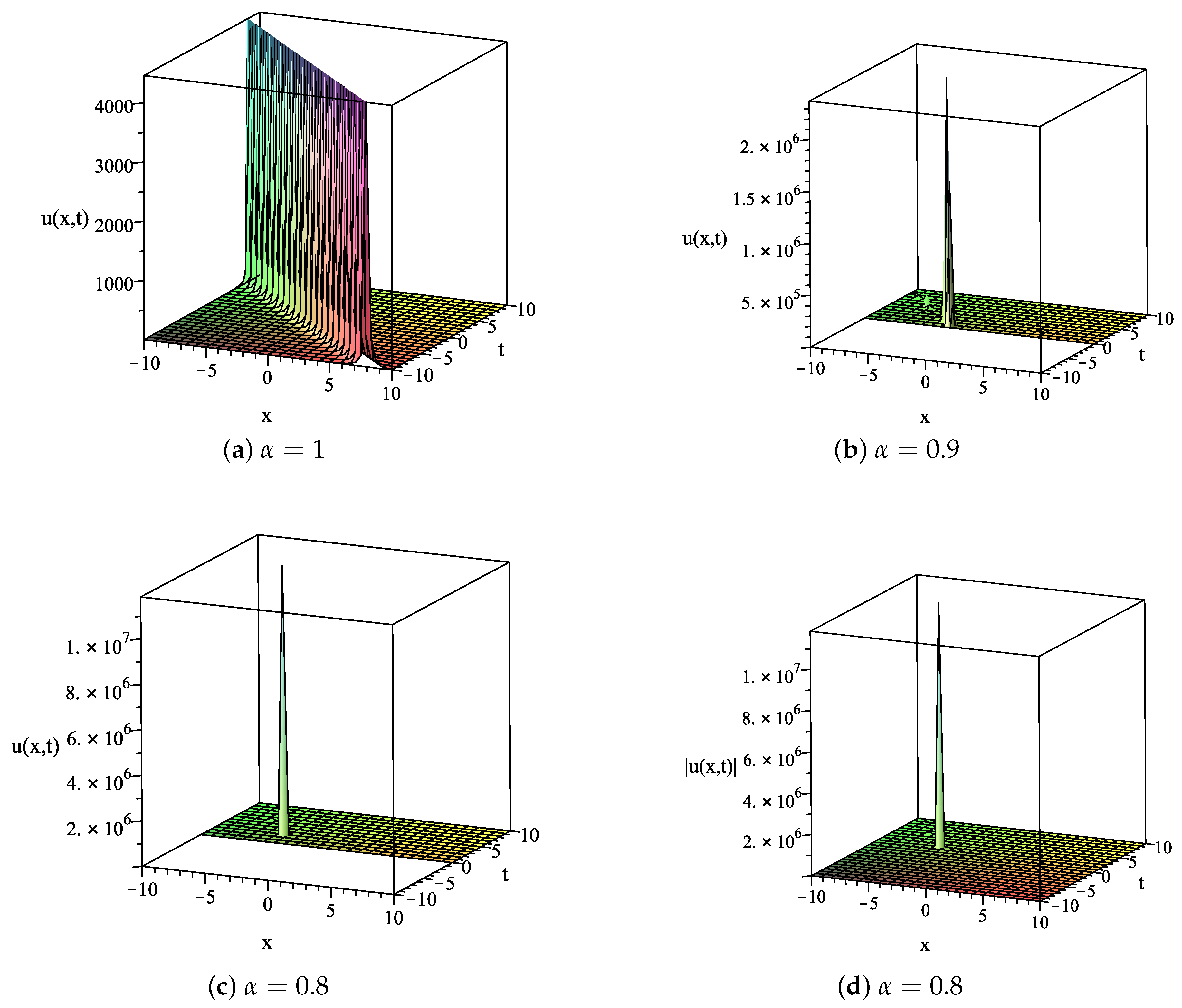
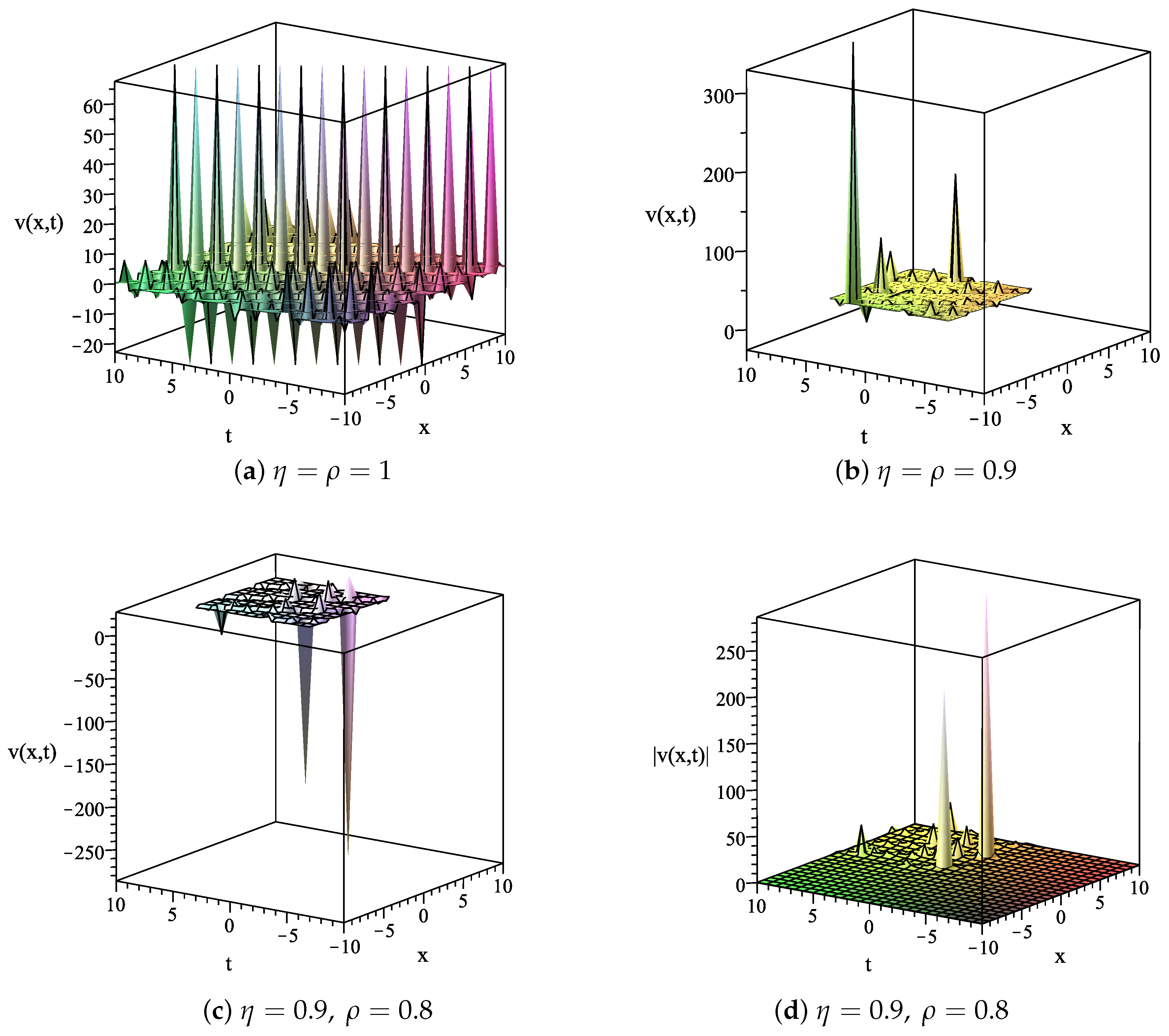
4.1. The Time-Fractional (2+1)-Dimensional Extended Quantum Zakharov-Kuznetsov Equation

Applying the transformation $\xi =-k\frac{t^{\alpha }}{\alpha }+x+y$ to Equation (1), we attain the following ordinary differential equation

$$\begin{array}{c}\hfill -k{U}^{\prime }+aU{U}^{\prime }+2(b+c)U^{‴}=0.\end{array}$$

(18)

Integrating (18) with respect to $\xi$, it gives

$$\begin{array}{c}\hfill -kU+\frac{a}{2}{U}^2+2(b+c)U^{″}+p=0,\end{array}$$

(19)

where p is a constant of integration. Applying the homogeneous balance principle to the terms $U^2$ and $U^{″}$ in Equation (18), we obtain $N=2$. Hence, the specific form of the solution in Equation (16) is written as

$$\begin{array}{c}\hfill U\left(\xi \right)=a_0+a_1\varphi \left(\xi \right)+a_2\varphi {\left(\xi \right)}^2+b_1\psi \left(\xi \right)+b_2\psi \left(\xi \right)\varphi \left(\xi \right),\end{array}$$

(20)

where the constant coefficients $a_0,a_1,a_2,b_1$, and $b_2$ are determined at a later step, provided that $a_2^2+b_2^2\ne 0$. Using the $(G{}^{\prime }/G,1/G)$-expansion method, there are three cases of the function $G\left(\xi \right)$ associated with the functions $\varphi \left(\xi \right)$ and $\psi \left(\xi \right)$, depending on the sign of $\lambda$ in Equation (7) as described above.

Case 1: Hyperbolic function solutions ($\mathbf{\lambda }<\mathbf{0}$)

If $\lambda <0$, we substitute Equation (20) into Equation (19) along with the use of Equation (9) and Equation (11). Then, the left-hand side of (19) turns out to be a polynomial in $\varphi \left(\xi \right)$ and $\psi \left(\xi \right)$. Equating all the coefficients of the resulting polynomial to be zero, we obtain the following system of nonlinear algebraic equations in $a_0,a_1,a_2,b_1,b_2,A_1,A_2,\lambda ,\mu ,k,$ and p, provided that ${\lambda }^2\left(A_1^2-A_2^2\right)+{\mu }^2\ne 0$.

$$\begin{array}{c}\hfill \begin{array}{cc}\hfill {\varphi }^4\left(\xi \right)& :2a{\lambda }^2{A}_1^2{a}_1{b}_2+2a{\lambda }^2{A}_1^2{a}_2{b}_1-2a{\lambda }^2{A}_2^2{a}_1{b}_2-2a{\lambda }^2{A}_2^2{a}_2{b}_1-40b{\lambda }^2\mu A_1^2{a}_2+8c{\mu }^2{b}_1\hfill \\ & +40b{\lambda }^2\mu A_2^2{a}_2-40c{\lambda }^2\mu A_1^2{a}_2+40c{\lambda }^2\mu A_2^2{a}_2+8b{\lambda }^2{A}_1^2{b}_1-8b{\lambda }^2{A}_2^2{b}_1+8c{\lambda }^2{A}_1^2{b}_1\hfill \\ & -8c{\lambda }^2{A}_2^2{b}_1+2a\lambda \mu b_2^2+2a{\mu }^2{a}_1{b}_2+2a{\mu }^2{a}_2{b}_1-40b{\mu }^3{a}_2-40c{\mu }^3{a}_2+8b{\mu }^2{b}_1=0,\hfill \\ \hfill {\varphi }^3\left(\xi \right)& :2a{\lambda }^2{A}_1^2{a}_1{a}_2-2a{\lambda }^2{A}_2^2{a}_1{a}_2+8b{\lambda }^2{A}_1^2{a}_1-8b{\lambda }^2{A}_2^2{a}_1+8c{\lambda }^2{A}_1^2{a}_1-8c{\lambda }^2{A}_2^2{a}_1\hfill \\ & +2a{\mu }^2{a}_1{a}_2-2a\lambda b_1{b}_2+24b\lambda \mu b_2+8b{\mu }^2{a}_1+24c\lambda \mu b_2+8c{\mu }^2{a}_1=0,\hfill \\ \hfill {\varphi }^3\left(\xi \right)\psi \left(\xi \right)& :2a{\lambda }^2{A}_1^2{a}_2{b}_2-2a{\lambda }^2{A}_2^2{a}_2{b}_2+24b{\lambda }^2{A}_1^2{b}_2-24b{\lambda }^2{A}_2^2{b}_2+24c{\lambda }^2{A}_1^2{b}_2-24c{\lambda }^2{A}_2^2{b}_2\hfill \\ & +2a{\mu }^2{a}_2{b}_2+24b{\mu }^2{b}_2+24c{\mu }^2{b}_2=0,\hfill \\ \hfill {\varphi }^2\left(\xi \right)& :2a{\lambda }^2{A}_1^2{a}_0{a}_2+a{\lambda }^2{A}_1^2{a}_1^2-2a{\lambda }^2{A}_2^2{a}_0{a}_2-a{\lambda }^2{A}_2^2{a}_1^2+32b{\lambda }^3{A}_1^2{a}_2-32b{\lambda }^3{A}_2^2{a}_2\hfill \\ & +32c{\lambda }^3{A}_1^2{a}_2-32c{\lambda }^3{A}_2^2{a}_2-2k{\lambda }^2{A}_1^2{a}_2+2k{\lambda }^2{A}_2^2{a}_2-a{\lambda }^2{b}_2^2+2a{\mu }^2{a}_0{a}_2+a{\mu }^2{a}_1^2\hfill \\ & +24b\lambda {\mu }^2{a}_2+24c\lambda {\mu }^2{a}_2-a\lambda b_1^2+4b\lambda \mu b_1+4c\lambda \mu b_1-2k{\mu }^2{a}_2=0,\hfill \\ \hfill {\varphi }^2\left(\xi \right)\psi \left(\xi \right)& :2a{\lambda }^2{A}_1^2{a}_1{b}_2+2a{\lambda }^2{A}_1^2{a}_2{b}_1-2a{\lambda }^2{A}_2^2{a}_1{b}_2-2a{\lambda }^2{A}_2^2{a}_2{b}_1-40b{\lambda }^2\mu A_1^2{a}_2+2a\lambda \mu b_2^2\hfill \\ & -40c{\lambda }^2\mu A_1^2{a}_2+40c{\lambda }^2\mu A_2^2{a}_2+8b{\lambda }^2{A}_1^2{b}_1-8b{\lambda }^2{A}_2^2{b}_1+8c{\lambda }^2{A}_1^2{b}_1-8c{\lambda }^2{A}_2^2{b}_1\hfill \\ & +2a{\mu }^2{a}_1{b}_2+2a{\mu }^2{a}_2{b}_1-40b{\mu }^3{a}_2-40c{\mu }^3{a}_2+8b{\mu }^2{b}_1+8c{\mu }^2{b}_1+40b{\lambda }^2\mu A_2^2{a}_2=0,\hfill \\ \hfill \varphi \left(\xi \right)& :2a{\lambda }^2{A}_1^2{a}_0{a}_1-2a{\lambda }^2{A}_2^2{a}_0{a}_1+8b{\lambda }^3{A}_1^2{a}_1-8b{\lambda }^3{A}_2^2{a}_1+8c{\lambda }^3{A}_1^2{a}_1-8c{\lambda }^3{A}_2^2{a}_1\hfill \\ & -2k{\lambda }^2{A}_1^2{a}_1+2k{\lambda }^2{A}_2^2{a}_1-2a{\lambda }^2{b}_1{b}_2+2a{\mu }^2{a}_0{a}_1+24b{\lambda }^2\mu b_2+8b\lambda {\mu }^2{a}_1+24c{\lambda }^2\mu b_2\hfill \\ & +8c\lambda {\mu }^2{a}_1-2k{\mu }^2{a}_1=0,\hfill \\ \hfill \varphi \left(\xi \right)\psi \left(\xi \right)& :2a{\lambda }^2{A}_1^2{a}_0{b}_2+2a{\lambda }^2{A}_1^2{a}_1{b}_1-2a{\lambda }^2{A}_2^2{a}_0{b}_2-2a{\lambda }^2{A}_2^2{a}_1{b}_1+20b{\lambda }^3{A}_1^2{b}_2-20b{\lambda }^3{A}_2^2{b}_2\hfill \\ & -12b{\lambda }^2\mu A_1^2{a}_1+12b{\lambda }^2\mu A_2^2{a}_1+20c{\lambda }^3{A}_1^2{b}_2-20c{\lambda }^3{A}_2^2{b}_2-12c{\lambda }^2\mu A_1^2{a}_1-2k{\mu }^2{b}_2\hfill \\ & -2k{\lambda }^2{A}_1^2{b}_2+2k{\lambda }^2{A}_2^2{b}_2+4a\lambda \mu b_1{b}_2+2a{\mu }^2{a}_0{b}_2+2a{\mu }^2{a}_1{b}_1-28b\lambda {\mu }^2{b}_2-12b{\mu }^3{a}_1\hfill \\ & -28c\lambda {\mu }^2{b}_2-12c{\mu }^3{a}_1+12c{\lambda }^2\mu A_2^2{a}_1=0,\hfill \\ \hfill \psi \left(\xi \right)& :-16b{\lambda }^3\mu A_1^2{a}_2+16b{\lambda }^3\mu A_2^2{a}_2-16c{\lambda }^3\mu A_1^2{a}_2+16c{\lambda }^3\mu A_2^2{a}_2+2a{\lambda }^2{A}_1^2{a}_0{b}_1\hfill \\ & -2a{\lambda }^2{A}_2^2{a}_0{b}_1+4b{\lambda }^3{A}_1^2{b}_1-4b{\lambda }^3{A}_2^2{b}_1+4c{\lambda }^3{A}_1^2{b}_1-4c{\lambda }^3{A}_2^2{b}_1-2k{\lambda }^2{A}_1^2{b}_1\hfill \\ & +2k{\lambda }^2{A}_2^2{b}_1+2a\lambda \mu b_1^2+2a{\mu }^2{a}_0{b}_1-4b\lambda {\mu }^2{b}_1-4c\lambda {\mu }^2{b}_1-2k{\mu }^2{b}_1=0,\hfill \\ \hfill \varphi {\left(\xi \right)}^0& :8b{\lambda }^4{A}_1^2{a}_2-8b{\lambda }^4{A}_2^2{a}_2+8c{\lambda }^4{A}_1^2{a}_2-8c{\lambda }^4{A}_2^2{a}_2+a{\lambda }^2{A}_1^2{a}_0^2-a{\lambda }^2{A}_2^2{a}_0^2-2{\lambda }^{2}p{A}_2^2\hfill \\ & -2k{\lambda }^2{A}_1^2{a}_0+2k{\lambda }^2{A}_2^2{a}_0-a{\lambda }^2{b}_1^2+a{\mu }^2{a}_0^2+4b{\lambda }^2\mu b_1+4c{\lambda }^2\mu b_1+2{\lambda }^{2}p{A}_1^2+2{\mu }^{2}p\hfill \\ & -2k{\mu }^2{a}_0=0.\hfill \end{array}\end{array}$$

(21)

Using the Maple package program to solve the above algebraic system, we obtain the following results.

Result 1:

$$\begin{array}{c}\hfill \begin{array}{c}{a}_0=-\frac{16(b+c)-k}{a},a_1=0,a_2=-\frac{24(b+c)}{a},b_1=0,b_2=0,\hfill \\ p=-\frac{64{\left(b+c\right)}^2{\lambda }^2-k^2}{2a},\mu =0,\lambda =\lambda ,k=k,\hfill \end{array}\end{array}$$

(22)

where $a\ne 0,b,c,\lambda (<0),\mu ,k$ are arbitrary constants. From Equations (10), (20), and (22), we obtain the traveling wave solution of Equation (1) as follows:

$$\begin{array}{c}\hfill \begin{array}{cc}\hfill u(x,y,t)& =-\frac{16(b+c)+k}{a}+\frac{24\lambda {\left(cosh\left(\xi \sqrt{-\lambda }\right)A_1+sinh\left(\xi \sqrt{-\lambda }\right)A_2\right)}^2\left(b+c\right)}{{\left(A_{1}sinh\left(\xi \sqrt{-\lambda }\right)+A_{2}cosh\left(\xi \sqrt{-\lambda }\right)\right)}^{2}a},\hfill \end{array}\end{array}$$

(23)

where $\xi =-k\frac{t^{\alpha }}{\alpha }+x+y$ and $A_1,A_2$ are arbitrary constants.

Result 2:

$$\begin{array}{c}\hfill \begin{array}{c}{a}_0=a_0,a_1=0,a_2=-\frac{12\left(b+c\right)}{a},b_1=\frac{12\mu \left(b+c\right)}{a},b_2=\pm \frac{12(b+c)}{a}\sqrt{\frac{-{\sigma }_1{\lambda }^2-{\mu }^2}{\lambda }},\hfill \\ p=\frac{\left(12\lambda \left(b+c\right)+a{a}_0\right)\left(8\lambda \left(b+c\right)+a{a}_0\right)}{2a},\mu =\mu ,\lambda =\lambda ,k=a{a}_0+10b\lambda +10c\lambda ,\hfill \end{array}\end{array}$$

(24)

where $a_0,a\ne 0,b,c,\lambda (<0),\mu$ are arbitrary constants and ${\sigma }_1=A_1^2-A_2^2,$ where $A_1,A_2$ are arbitrary constants. From Equations (12), (20), and (24), we obtain the exact solution of Equation (1) as follows:

$$\begin{array}{c}\hfill \begin{array}{cc}\hfill u(x,y,t)& =a_0+\frac{{12\lambda }^3{\left(cosh\left(\xi \sqrt{-\lambda }\right)A_1+sinh\left(\xi \sqrt{-\lambda }\right)A_2\right)}^2\left(b+c\right)}{{\left(A_{2}cosh\left(\xi \sqrt{-\lambda }\right)\lambda +A_{1}sinh\left(\xi \sqrt{-\lambda }\right)\lambda +\mu \right)}^{2}a}\hfill \\ & +\frac{12\lambda \mu \left(b+c\right)}{\left(A_{2}cosh\left(\xi \sqrt{-\lambda }\right)\lambda +A_{1}sinh\left(\xi \sqrt{-\lambda }\right)\lambda +\mu \right)a}\hfill \\ & \mp \frac{12{\left(-\lambda \right)}^{3/2}\sqrt{\lambda }\left(cosh\left(\xi \sqrt{-\lambda }\right)A_1+sinh\left(\xi \sqrt{-\lambda }\right)A_2\right)\sqrt{{-{\sigma }_1\lambda }^2-{\mu }^2}\left(b+c\right)}{{\left(A_{2}cosh\left(\xi \sqrt{-\lambda }\right)\lambda +A_{1}sinh\left(\xi \sqrt{-\lambda }\right)\lambda +\mu \right)}^{2}a},\hfill \end{array}\end{array}$$

(25)

where $\xi =-k\frac{t^{\alpha }}{\alpha }+x+y$ with k defined in Equation (24).

Case 2: Trigonometric function solutions ($\mathbf{\lambda }>\mathbf{0}$)

If $\lambda >0$, we insert Equation (20) into Equation (19) along with the use of Equations (9) and (13). Then, the left-hand side of (19) becomes a polynomial in $\varphi \left(\xi \right)$ and $\psi \left(\xi \right)$. Setting all of coefficients of this resulting polynomial to be zero, we have the following system of nonlinear algebraic equations in $a_0,a_1,a_2,b_1,b_2,A_1,A_2,\lambda ,\mu ,k,$ and p, provided that ${\lambda }^2\left(A_1^2+A_2^2\right)-{\mu }^2\ne 0$.

$$\begin{array}{c}\hfill \begin{array}{cc}\hfill {\varphi }^4\left(\xi \right)& :a{\lambda }^2{A}_1^2{a}_2^2+a{\lambda }^2{A}_2^2{a}_2^2+24b{\lambda }^2{A}_1^2{a}_2+24b{\lambda }^2{A}_2^2{a}_2+24c{\lambda }^2{A}_1^2{a}_2+24c{\lambda }^2{A}_2^2{a}_2\hfill \\ & -a{\mu }^2{a}_2^2+a\lambda b_2^2-24b{\mu }^2{a}_2-24c{\mu }^2{a}_2=0,\hfill \\ \hfill {\varphi }^3\left(\xi \right)& :2a{\lambda }^2{A}_1^2{a}_1{a}_2+2a{\lambda }^2{A}_2^2{a}_1{a}_2+8b{\lambda }^2{A}_1^2{a}_1+8b{\lambda }^2{A}_2^2{a}_1+8c{\lambda }^2{A}_1^2{a}_1+8c{\lambda }^2{A}_2^2{a}_1\hfill \\ & -2a{\mu }^2{a}_1{a}_2+2a\lambda b_1{b}_2-24b\lambda \mu b_2-8b{\mu }^2{a}_1-24c\lambda \mu b_2-8c{\mu }^2{a}_1=0,\hfill \\ \hfill {\varphi }^3\left(\xi \right)\psi \left(\xi \right)& :2a{\lambda }^2{A}_1^2{a}_2{b}_2+2a{\lambda }^2{A}_2^2{a}_2{b}_2+24b{\lambda }^2{A}_1^2{b}_2+24b{\lambda }^2{A}_2^2{b}_2+24c{\lambda }^2{A}_1^2{b}_2+24c{\lambda }^2{A}_2^2{b}_2\hfill \\ & -2a{\mu }^2{a}_2{b}_2-24b{\mu }^2{b}_2-24c{\mu }^2{b}_2=0,\hfill \\ \hfill {\varphi }^2\left(\xi \right)& :2a{\lambda }^2{A}_1^2{a}_0{a}_2+a{\lambda }^2{A}_1^2{a}_1^2+2a{\lambda }^2{A}_2^2{a}_0{a}_2+a{\lambda }^2{A}_2^2{a}_1^2+32b{\lambda }^3{A}_1^2{a}_2+32b{\lambda }^3{A}_2^2{a}_2\hfill \\ & +32c{\lambda }^3{A}_1^2{a}_2+32c{\lambda }^3{A}_2^2{a}_2-2k{\lambda }^2{A}_1^2{a}_2-2k{\lambda }^2{A}_2^2{a}_2+a{\lambda }^2{b}_2^2-2a{\mu }^2{a}_0{a}_2-a{\mu }^2{a}_1^2\hfill \\ & -24b\lambda {\mu }^2{a}_2-24c\lambda {\mu }^2{a}_2+a\lambda b_1^2-4b\lambda \mu b_1-4c\lambda \mu b_1+2k{\mu }^2{a}_2=0,\hfill \\ \hfill {\varphi }^2\left(\xi \right)\psi \left(\xi \right)& :2a{\lambda }^2{A}_1^2{a}_1{b}_2+2a{\lambda }^2{A}_1^2{a}_2{b}_1+2a{\lambda }^2{A}_2^2{a}_1{b}_2+2a{\lambda }^2{A}_2^2{a}_2{b}_1-40b{\lambda }^2\mu A_1^2{a}_2-8c{\mu }^2{b}_1\hfill \\ & -40b{\lambda }^2\mu A_2^2{a}_2-40c{\lambda }^2\mu A_1^2{a}_2-40c{\lambda }^2\mu A_2^2{a}_2+8b{\lambda }^2{A}_1^2{b}_1+8b{\lambda }^2{A}_2^2{b}_1+8c{\lambda }^2{A}_1^2{b}_1\hfill \\ & +8c{\lambda }^2{A}_2^2{b}_1-2a\lambda \mu b_2^2-2a{\mu }^2{a}_1{b}_2-2a{\mu }^2{a}_2{b}_1+40b{\mu }^3{a}_2+40c{\mu }^3{a}_2-8b{\mu }^2{b}_1=0,\hfill \\ \hfill \varphi \left(\xi \right)& :2a{\lambda }^2{A}_1^2{a}_0{a}_1+2a{\lambda }^2{A}_2^2{a}_0{a}_1+8b{\lambda }^3{A}_1^2{a}_1+8b{\lambda }^3{A}_2^2{a}_1+8c{\lambda }^3{A}_1^2{a}_1+8c{\lambda }^3{A}_2^2{a}_1\hfill \\ & -2k{\lambda }^2{A}_1^2{a}_1-2k{\lambda }^2{A}_2^2{a}_1+2a{\lambda }^2{b}_1{b}_2-2a{\mu }^2{a}_0{a}_1-24b{\lambda }^2\mu b_2-8b\lambda {\mu }^2{a}_1-24c{\lambda }^2\mu b_2\hfill \\ & -8c\lambda {\mu }^2{a}_1+2k{\mu }^2{a}_1=0,\hfill \\ \hfill \varphi \left(\xi \right)\psi \left(\xi \right)& :2a{\lambda }^2{A}_1^2{a}_0{b}_2+2a{\lambda }^2{A}_1^2{a}_1{b}_1+2a{\lambda }^2{A}_2^2{a}_0{b}_2+2a{\lambda }^2{A}_2^2{a}_1{b}_1+20b{\lambda }^3{A}_1^2{b}_2+2k{\mu }^2{b}_2\hfill \\ & +20b{\lambda }^3{A}_2^2{b}_2-12b{\lambda }^2\mu A_1^2{a}_1-12b{\lambda }^2\mu A_2^2{a}_1+20c{\lambda }^3{A}_1^2{b}_2+20c{\lambda }^3{A}_2^2{b}_2+12c{\mu }^3{a}_1\hfill \\ & -12c{\lambda }^2\mu A_1^2{a}_1-12c{\lambda }^2\mu A_2^2{a}_1-2k{\lambda }^2{A}_1^2{b}_2-2k{\lambda }^2{A}_2^2{b}_2-4a\lambda \mu b_1{b}_2-2a{\mu }^2{a}_0{b}_2\hfill \\ & -2a{\mu }^2{a}_1{b}_1+28b\lambda {\mu }^2{b}_2+12b{\mu }^3{a}_1+28c\lambda {\mu }^2{b}_2=0,\hfill \\ \hfill \psi \left(\xi \right)& :-16b{\lambda }^3\mu A_1^2{a}_2-16b{\lambda }^3\mu A_2^2{a}_2-16c{\lambda }^3\mu A_1^2{a}_2-16c{\lambda }^3\mu A_2^2{a}_2+2a{\lambda }^2{A}_1^2{a}_0{b}_1\hfill \\ & +2a{\lambda }^2{A}_2^2{a}_0{b}_1+4b{\lambda }^3{A}_1^2{b}_1+4b{\lambda }^3{A}_2^2{b}_1+4c{\lambda }^3{A}_1^2{b}_1+4c{\lambda }^3{A}_2^2{b}_1-2k{\lambda }^2{A}_1^2{b}_1\hfill \\ & -2k{\lambda }^2{A}_2^2{b}_1-2a\lambda \mu b_1^2-2a{\mu }^2{a}_0{b}_1+4b\lambda {\mu }^2{b}_1+4c\lambda {\mu }^2{b}_1+2k{\mu }^2{b}_1=0,\hfill \\ \hfill \varphi {\left(\xi \right)}^0& :8b{\lambda }^4{A}_1^2{a}_2+8b{\lambda }^4{A}_2^2{a}_2+8c{\lambda }^4{A}_1^2{a}_2+8c{\lambda }^4{A}_2^2{a}_2+a{\lambda }^2{A}_1^2{a}_0^2+a{\lambda }^2{A}_2^2{a}_0^2-2{\mu }^{2}p\hfill \\ & -2k{\lambda }^2{A}_1^2{a}_0-2k{\lambda }^2{A}_2^2{a}_0+a{\lambda }^2{b}_1^2-a{\mu }^2{a}_0^2-4b{\lambda }^2\mu b_1-4c{\lambda }^2\mu b_1+2{\lambda }^{2}p{A}_1^2\hfill \\ & +2k{\mu }^2{a}_0+2{\lambda }^{2}p{A}_2^2=0.\hfill \end{array}\end{array}$$

(26)

By solving the above algebraic system using the Maple package program, we obtain the following results.

Result 1:

$$\begin{array}{c}\hfill \begin{array}{c}{a}_0=-\frac{16(b+c)-k}{a},a_1=0,a_2=-\frac{24(b+c)}{a},b_1=0,b_2=0,\hfill \\ p=-\frac{64{\left(b+c\right)}^2{\lambda }^2-k^2}{2a},\mu =0,\lambda =\lambda ,k=k,\hfill \end{array}\end{array}$$

(27)

where $a\ne 0,b,c,\lambda (>0),k$ are arbitrary constants. From Equations (12), (20) and (27), we obtain the exact solution of Equation (1) as follows:

$$\begin{array}{c}\hfill \begin{array}{cc}\hfill u(x,y,t)& =-\frac{16(b+c)-k}{a}-\frac{24\lambda {\left(cos\left(\xi \sqrt{\lambda }\right)A_1-sin\left(\xi \sqrt{\lambda }\right)A_2\right)}^2\left(b+c\right)}{{\left(A_{1}sin\left(\xi \sqrt{\lambda }\right)+A_{2}cos\left(\xi \sqrt{\lambda }\right)\right)}^{2}a},\hfill \end{array}\end{array}$$

(28)

where $\xi =-k\frac{t^{\alpha }}{\alpha }+x+y$ and $A_1,A_2$ are arbitrary constants.

Result 2:

$$\begin{array}{c}\hfill \begin{array}{c}{a}_0=a_0,a_1=0,a_2=-\frac{12(b+c)}{a},b_1=\frac{12\mu \left(b+c\right)}{a},b_2=\pm \frac{12(b+c)}{a}\sqrt{\frac{{\sigma }_2{\lambda }^2-{\mu }^2}{\lambda }},\hfill \\ p=\frac{\left(12\lambda \left(b+c\right)+a{a}_0\right)\left(8\lambda \left(b+c\right)+a{a}_0\right)}{2a},\mu =\mu ,\lambda =\lambda ,k=a{a}_0+10b\lambda +10c\lambda ,\hfill \end{array}\end{array}$$

(29)

where $a_0,a\ne 0,b,c,\lambda (>0),\mu$ are arbitrary constants and ${\sigma }_2=A_1^2+A_2^2,$ where $A_1,A_2$ are arbitrary constants. From Equations (12), (20), and (29), we obtain the exact solution of Equation (1) as follows:

$$\begin{array}{c}\hfill \begin{array}{cc}\hfill u(x,y,t)& =a_0-\frac{12{\lambda }^3{\left(cos\left(\xi \sqrt{\lambda }\right)A_1-sin\left(\xi \sqrt{\lambda }\right)A_2\right)}^2\left(b+c\right)}{{\left(A_{2}cos\left(\xi \sqrt{\lambda }\right)\lambda +A_{1}sin\left(\xi \sqrt{\lambda }\right)\lambda +\mu \right)}^{2}a}\hfill \\ & +\frac{12\lambda \mu \left(b+c\right)}{\left(A_{2}cos\left(\xi \sqrt{\lambda }\right)\lambda +A_{1}sin\left(\xi \sqrt{\lambda }\right)\lambda +\mu \right)a}\hfill \\ & \pm \frac{12{\lambda }^{5/2}\left(cos\left(\xi \sqrt{\lambda }\right)A_1-sin\left(\xi \sqrt{\lambda }\right)A_2\right)\sqrt{{\sigma }_2{\lambda }^2-{\mu }^2}\left(b+c\right)}{{\left(A_{2}cos\left(\xi \sqrt{\lambda }\right)\lambda +A_{1}sin\left(\xi \sqrt{\lambda }\right)\lambda +\mu \right)}^{2}a},\hfill \end{array}\end{array}$$

(30)

where $\xi =-k\frac{t^{\alpha }}{\alpha }+x+y$ with k defined in Equation (29).

Case 3: Rational function solutions ($\mathbf{\lambda }=\mathbf{0}$)

If $\lambda =0$, we substitute Equation (20) into Equation (19) along with the use of Equations (9) and (15). Then, the left-hand side of (19) becomes a polynomial in variables $\varphi \left(\xi \right)$ and $\psi \left(\xi \right)$. Setting all of the coefficients of the resulting polynomial to be zero, we have the following system of nonlinear algebraic equations in $a_0,a_1,a_2,b_1,b_2,A_1,A_2,\lambda ,\mu ,k,$ and p, provided that $A_1^2-2\mu A_2\ne 0$.

$$\begin{array}{c}\hfill \begin{array}{cc}\hfill {\varphi }^4\left(\xi \right)& :-2a\mu A_2{a}_2^2+a{A}_1^2{a}_2^2-48b\mu A_2{a}_2+24b{A}_1^2{a}_2-48c\mu A_2{a}_2+24c{A}_1^2{a}_2+a{b}_2^2=0,\hfill \\ \hfill {\varphi }^3\left(\xi \right)& :-4a\mu A_2{a}_1{a}_2+2a{A}_1^2{a}_1{a}_2-16b\mu A_2{a}_1+8b{A}_1^2{a}_1-16c\mu A_2{a}_1+8c{A}_1^2{a}_1+2a{b}_1{b}_2\hfill \\ & -24b\mu b_2-24c\mu b_2=0,\hfill \\ \hfill {\varphi }^3\left(\xi \right)\psi \left(\xi \right)& :-4a\mu A_2{a}_2{b}_2+2a{A_1}^2{a}_2{b}_2-48b\mu A_2{b}_2+24b{A}_1^2{b}_2-48c\mu A_2{b}_2+24c{A}_1^2{b}_2=0,\hfill \\ \hfill {\varphi }^2\left(\xi \right):& -4a\mu A_2{a}_0{a}_2-2a\mu A_2{a}_1^2+2a{A}_1^2{a}_0{a}_2+a{A}_1^2{a}_1^2+8b{\mu }^2{a}_2+8c{\mu }^2{a}_2+4k\mu A_2{a}_2\hfill \\ & -2k{A}_1^2{a}_2+a{b}_1^2-4b\mu b_1-4c\mu b_1=0,\hfill \\ \hfill {\varphi }^2\left(\xi \right)\psi \left(\xi \right)& :-4a\mu A_2{a}_1{b}_2-4a\mu A_2{a}_2{b}_1+2a{A}_1^2{a}_1{b}_2+2a{A}_1^2{a}_2{b}_1+80b{\mu }^2{A}_2{a}_2-40b\mu A_1^2{a}_2\hfill \\ & +80c{\mu }^2{A}_2{a}_2-40c\mu A_1^2{a}_2-2a\mu b_2^2-16b\mu A_2{b}_1+8b{A}_1^2{b}_1-16c\mu A_2{b}_1+8c{A_1}^2{b}_1=0,\hfill \\ \hfill \varphi \left(\xi \right)& :-4a\mu A_2{a}_0{a}_1+2a{A}_1^2{a}_0{a}_1+4k\mu A_2{a}_1-2k{A}_1^2{a}_1=0,\hfill \\ \hfill \varphi \left(\xi \right)\psi \left(\xi \right)& :-4a\mu A_2{a}_0{b}_2-4a\mu A_2{a}_1{b}_1+2a{A}_1^2{a}_0{b}_2+2a{A}_1^2{a}_1{b}_1+24b{\mu }^2{A}_2{a}_1-12b\mu A_1^2{a}_1\hfill \\ & +24c{\mu }^2{A}_2{a}_1-12c\mu A_1^2{a}_1-4a\mu b_1{b}_2+48b{\mu }^2{b}_2+48c{\mu }^2{b}_2+4k\mu A_2{b}_2-2k{A}_1^2{b}_2=0,\hfill \\ \hfill \psi \left(\xi \right)& :-4a\mu A_2{a}_0{b}_1+2a{A}_1^2{a}_0{b}_1-16b{\mu }^3{a}_2-16c{\mu }^3{a}_2-2a\mu b_1^2+8b{\mu }^2{b}_1+8c{\mu }^2{b}_1+4k\mu A_2{b}_1\hfill \\ & -2k{A}_1^2{b}_1=0,\hfill \\ \hfill \varphi {\left(\xi \right)}^0& :-2a\mu A_2{a}_0^2+a{A}_1^2{a}_0^2+4k\mu A_2{a}_0-2k{A}_1^2{a}_0-4\mu p{A}_2+2p{A}_1^2=0.\hfill \end{array}\end{array}$$

(31)

On solving the above algrebraic system using the Maple package program, we obtain the following results.

Result 1:

$$\begin{array}{c}\hfill \begin{array}{c}{a}_0=a_0,a_1=0,a_2=-\frac{24(b+c)}{a},b_1=0,b_2=0,p=\frac{a{a}_0^2}{2},\mu =0,k=a{a}_0,\hfill \end{array}\end{array}$$

(32)

where $a_0,a\ne 0,b,c$ are arbitrary constants. From Equations (14), (20) and (32), we obtain the traveling wave solution of Equation (1) as follows:

$$\begin{array}{c}\hfill \begin{array}{cc}\hfill u(x,y,t)& =a_0-\frac{A_1^2\left(24b+24c\right)}{{\left(A_1\xi +A_2\right)}^{2}a},\hfill \end{array}\end{array}$$

(33)

where $\xi =-k\frac{t^{\alpha }}{\alpha }+x+y$ with k defined in Equation (32) and $A_1,A_2$ are arbitrary constants.

Result 2:

$$\begin{array}{c}\hfill \begin{array}{c}{a}_0=a_0,a_1=0,a_2=-\frac{12(b+c)}{a},b_1=\frac{144{\left(b+c\right)}^2{A}_1^2-a^2{b}_2^2}{24a{A}_2\left(b+c\right)},b_2=b_2,p=\frac{a{a}_0^2}{2},\hfill \\ \mu =\frac{b_{1}a}{12(b+c)},k=a{a}_0,\hfill \end{array}\end{array}$$

(34)

where $a_0,b_2,a,b,c,A_1,A_2$ are arbitrary constants such that $a{A}_2\left(b+c\right)\ne 0$. From Equations (14), (20), and (34), we obtain the traveling wave solution of Equation (1) as follows:

$$\begin{array}{c}\hfill \begin{array}{cc}\hfill u(x,y,t)& =-\frac{48\left(b+c\right){\left(12\left(b+c\right)A_1+b_{1}a\xi \right)}^2}{{\left(24A_1\xi \left(b+c\right)+b_{1}a{\xi }^2+24A_2\left(b+c\right)\right)}^{2}a}+\frac{24b_1\left(b+c\right)}{24A_1\xi \left(b+c\right)+b_{1}a{\xi }^2+24A_2\left(b+c\right)}\hfill \\ & +\frac{48b_2\left(b+c\right)\left(12\left(b+c\right)A_1+b_{1}a\xi \right)}{{\left(24A_1\xi \left(b+c\right)+b_{1}a{\xi }^2+24A_2\left(b+c\right)\right)}^2},\hfill \end{array}\end{array}$$

(35)

where $\xi =-k\frac{t^{\alpha }}{\alpha }+x+y$ with k defined in Equation (34).

In the following part, the selected exact solutions of Equation (1), which are expressed in Equations (25), (28) and (35), are plotted for the three-dimensional representations. They will be portrayed on $-10\le x,t\le 10$ by varying the fractional order $\alpha \in \{1,0.9,0.8\}.$ The graphical results are as follows.

The following fixed values $a_0=1,\mu =1,\lambda =-0.1,A_1=2,A_2=1,a=1,b=1,c=1$ and the variation of $\alpha \in \{1,0.9,0.8\}$ are utilized to plot associated graphs of $u(x,y,t)$ expressed in Equation (25). In Figure 1a, the solution $u(x,y,t)$ with $\alpha =1$ is plotted to describe the bell-shaped solitary wave solution. The graphs of the solution $u(x,y,t)$ for $\alpha =0.9$ and $\alpha =0.8$ are shown in Figure 1b,c, respectively. The graph of $\left|u\right(x,y,t\left)\right|$ for $\alpha =0.8$ is depicted in Figure 1d. Figure 1b,c cannot show a graphical representation for $-10<t<0$ since $u(x,y,t)$ is a complex-valued function on this interval.

In Figure 2a, the periodic traveling wave solution, obtained using the solution $u(x,y,t)$ in Equation (28), is displayed using the parameter values $k=1,\lambda =2,A_1=2,A_2=1,a=-1,$$b=1,c=1,$ and the fractional orders $\alpha =1$. Using the above parameter values, Figure 2b,c, represent the solution $u(x,y,t)$ describing singular soliton solutions for $\alpha =0.9$ and $\alpha =0.8$, respectively. The graph of $\left|u\right(x,y,t\left)\right|$ with $\alpha =0.8$ is portrayed in Figure 2d. We can observe that Figure 2b,c cannot give a graphical representation for $-10<t<0$, since $u(x,y,t)$ is a complex-valued function on this interval.

For the fixed values $a_0=1,b_2=1,A_1=2,A_2=1,a=-1,b=1,c=1,$ the graphs of the exact solutions $u(x,y,t)$ in Equation (35) of Equation (1) corresponding to the given variation of $\alpha$ are investigated. The solution $u(x,y,t)$ with $\alpha =1$, describing the solitary wave solution of singular soliton type, is depicted in Figure 3a. The solutions $u(x,y,t)$ with $\alpha =0.9$ and $\alpha =0.8$, showing the discontinuous singular single-soliton solution, are presented in Figure 3b,c, respectively. Since $u(x,y,t)$ is a complex-valued function on $-10<t<0$, then these figures do not present any graph for this interval. The graph of $\left|u\right(x,y,t\left)\right|$ with $\alpha =0.8$ is plotted in Figure 3d.

Next, we compare our exact solutions of Equation (1), achieved using the $(G^{\prime }/G,1/G)$-expansion method to the ones obtained using the different methods, which were reported before. In 2019, Ali et al., [37] analytically solved Equation (1) using the modified Kudryashov method and the $(G^{\prime }/G^2)$-expansion method. They found that the former method provided the two exact solutions written in terms of the reciprocal of exponential function solutions. The latter method, which they employed, released six sets of the coefficients and parameter values in which each set generated three classes of the solutions, including trigonometric, hyperbolic, and rational function solutions, while our results generated using the $(G^{\prime }/G,1/G)$-expansion method included two hyperbolic function solutions, two trigonometric function solutions, and two rational function solutions. When comparing the number of solution classes obtained using the $(G^{\prime }/G^2)$-expansion method and the $(G^{\prime }/G,1/G)$-expansion method, they are the same number. However, their solutions and our solutions are not exactly the same. Applying the $(G^{\prime }/G,1/G)$-expansion method to Equation (1), our solutions are new and distinct from the results in [37].

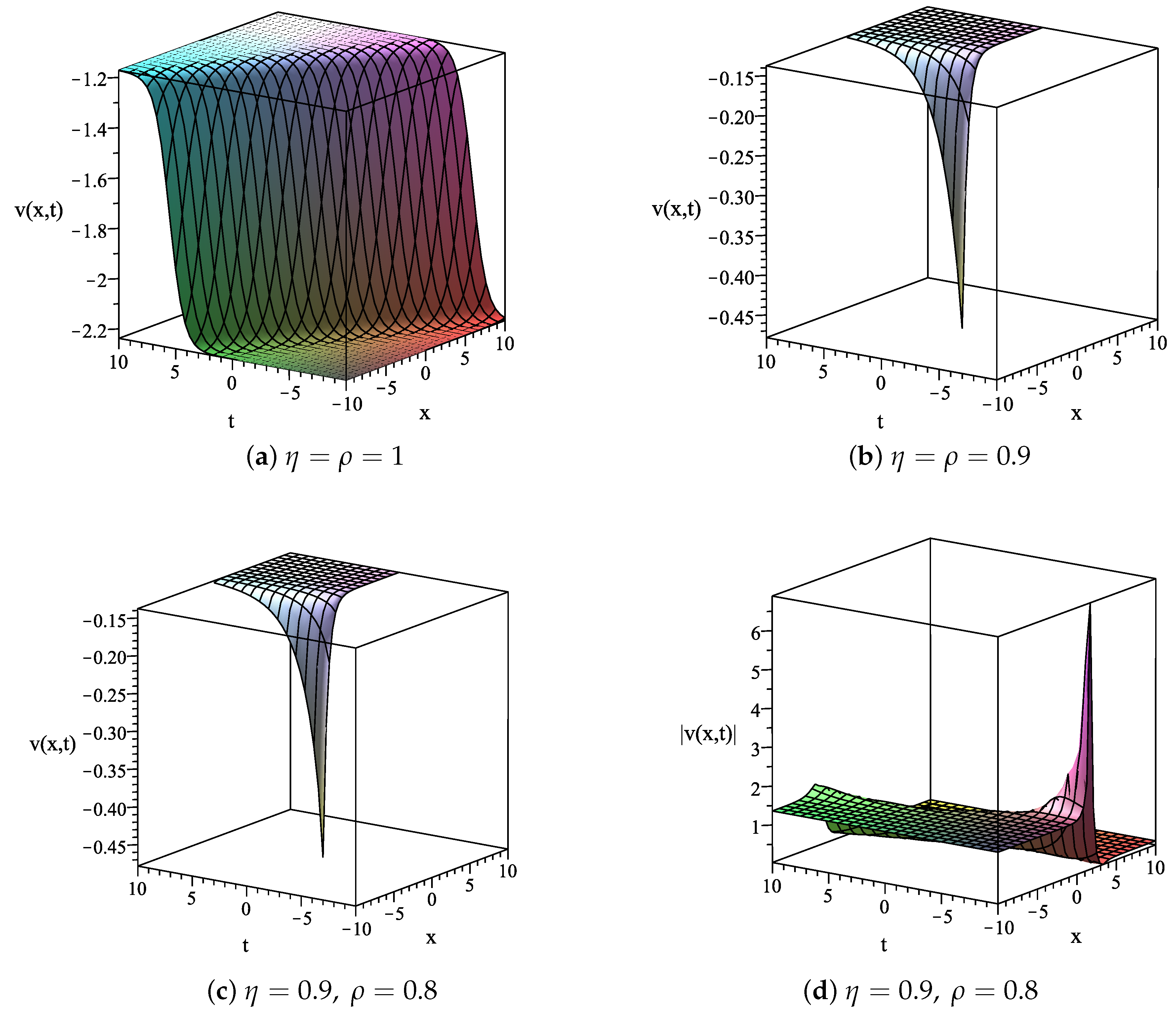
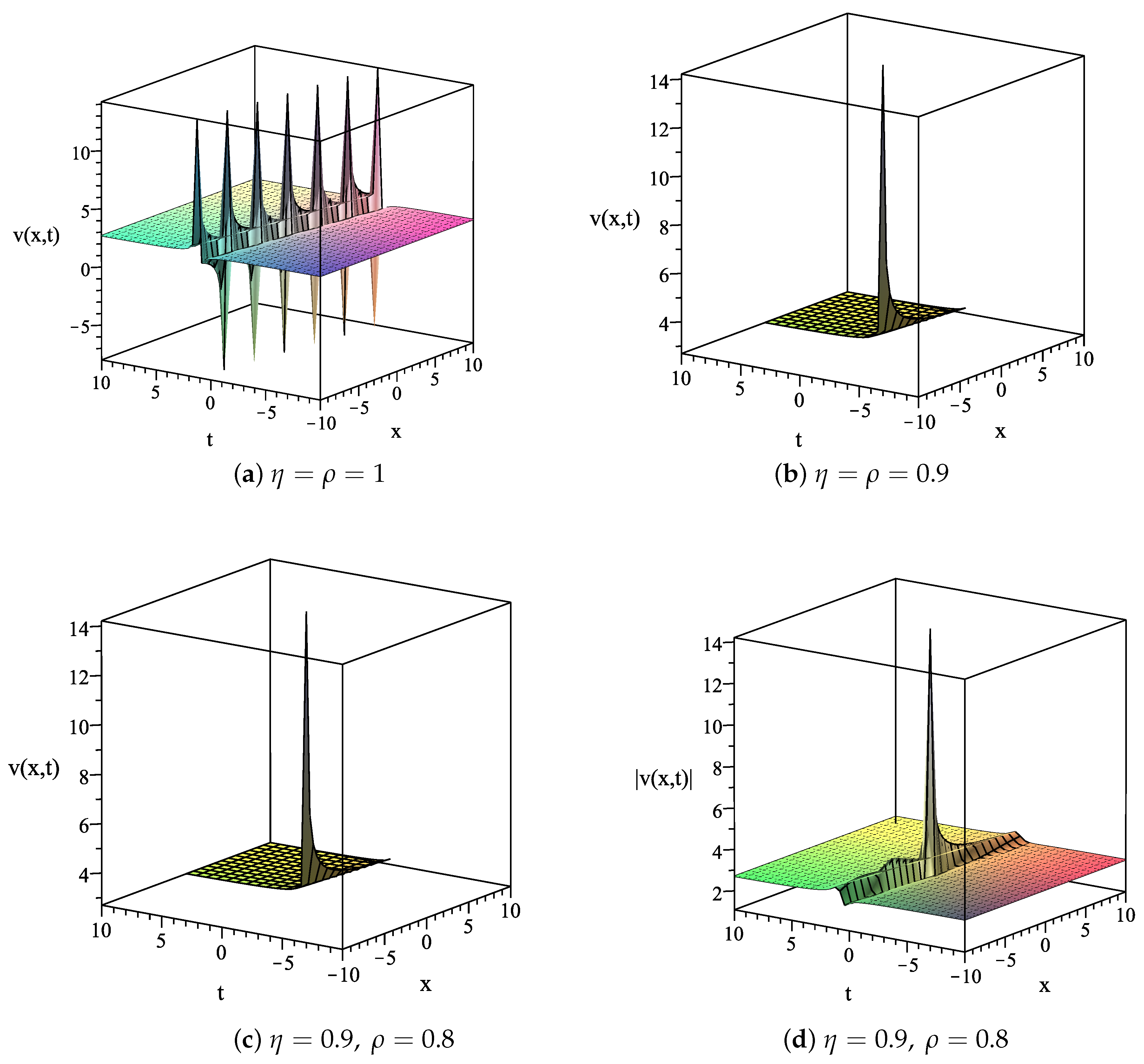
4.2. The Space-Time-Fractional Generalized Hirota-Satsuma Coupled KdV System

Before finding exact traveling wave solutions of the space-time-fractional generalized Hirota-Satsuma coupled KdV system in Equation (2) by using the $(G{}^{\prime }/G,1/G)$-expansion method, we must convert it to a system of ordinary differential equations using the following transformations

$$\begin{array}{c}\hfill u(x,t)=U\left(\xi \right),v(x,t)=V\left(\xi \right),w(x,t)=W\left(\xi \right),\xi =k\left(\frac{x^{\eta }}{\eta }-c\frac{t^{\rho }}{\rho }\right),\end{array}$$

(36)

where k and c are non-zero arbitrary constants to be determined later. Substituting Equation (36) into Equation (2), we yield a system of ODEs, as follows:

$$\begin{array}{ccc}\hfill -ck{U}^{\prime }& =& {\displaystyle \frac{1}{4}}{k}^3{U}^{‴}+3kU{U}^{\prime }+3k{(-V^2+W)}^{\prime },\hfill \end{array}$$

(37)

$$\begin{array}{ccc}\hfill -ck{V}^{\prime }& =& -{\displaystyle \frac{1}{2}}{k}^3{V}^{‴}-3kU{V}^{\prime },\hfill \end{array}$$

(38)

$$\begin{array}{ccc}\hfill -ck{W}^{\prime }& =& -{\displaystyle \frac{1}{2}}{k}^3{W}^{‴}-3kU{W}^{\prime }..\hfill \end{array}$$

(39)

Let [53]

$$\begin{array}{c}\hfill U=\alpha V^2+\beta V+\gamma ,W=AV+B,\end{array}$$

(40)

where $\alpha ,\beta ,\gamma ,A$ and B are constants to be determined later.

Substituting Equation (40) into Equations (38) and (39), and then integrating once, we know that Equations (38) and (39) give the same resulting equation as follows:

$$\begin{array}{c}\hfill k^{2}V{}^{″}=-2\alpha V^3-3\beta V^2+2(c-3\gamma )V+c_1,\end{array}$$

(41)

where $c_1$ is a constant of integration. Multiplying Equation (41) by $V^{\prime }$ and then integrating the resulting equation with respect to $\xi$, we obtain

$$\begin{array}{c}\hfill k^2{\left(V{}^{\prime }\right)}^2=-\alpha V^4-2\beta V^3+2(c-3\gamma )V^2+2c_{1}V+c_2,\end{array}$$

(42)

where $c_2$ is also a constant of integration.

Differentiating Equation (40) with respect to $\xi$ and then using Equations (41) and (42), we obtain

$$\begin{array}{ccc}\hfill k^{2}U{}^{″}& =& 2\alpha k^2{\left(V{}^{\prime }\right)}^2+k^2(2\alpha V+\beta )V{}^{″},\hfill \\ & =& 2\alpha \left[-\alpha V^4-2\beta V^3+2(c-3\gamma )V^2+2c_{1}V+c_2\right]\hfill \\ & & +(2\alpha V+\beta )\left[-2\alpha V^3-3\beta V^2+2(c-3\gamma )V+c_1\right].\hfill \end{array}$$

(43)

Integrating Equation (37) once, we get

$$\begin{array}{c}\hfill {\displaystyle \frac{1}{4}}{k}^{2}U{}^{″}+{\displaystyle \frac{3}{2}}{U}^2+cU+3(-V^2+W)+c_3=0,\end{array}$$

(44)

where $c_3$ is a constant of integration. Substituting Equations (40) and (43) into Equation (44), we obtain that the following coefficients of the resulting polynomial are zero, as follows:

$$\begin{array}{c}\hfill \begin{array}{ccc}\hfill 3\alpha c-3\alpha \gamma +{\displaystyle \frac{3}{4}}{\beta }^2-3& =\hfill & \hfill 0,\\ \hfill {\displaystyle \frac{1}{2}}\left(\alpha c_1+\beta c+\gamma \beta \right)+A& =\hfill & \hfill 0,\\ \hfill {\displaystyle \frac{1}{4}}\left(2\alpha c_2+\beta c_1\right)+{\displaystyle \frac{3}{2}}{\gamma }^2+c\gamma +3B+c_3& =\hfill & \hfill 0.\end{array}\end{array}$$

(45)

Let

$$\begin{array}{c}\hfill c_1=\frac{1}{2{\alpha }^2}({\beta }^3+2c\alpha \beta -6\alpha \beta \gamma ),V\left(\xi \right)=aP\left(\xi \right)-\frac{\beta }{2\alpha }.\end{array}$$

(46)

We find from (45) that

$$\begin{array}{cc}\hfill \alpha & =\frac{{\beta }^2-4}{4(\gamma -c)},A=\frac{4\beta (c-\gamma )}{{\beta }^2-4},\hfill \\ \hfill B& ={\displaystyle \frac{1}{6\left(-\gamma +c\right){\left({\beta }^2-4\right)}^2}}(16c_{3}c{\beta }^2-2c_{3}c{\beta }^4-16c_3\gamma {\beta }^2+2c_3\gamma {\beta }^4\hfill \\ & +56c^2\gamma {\beta }^2-48{\gamma }^{2}c{\beta }^2-16c_2+\frac{1}{4}{c}_2{\beta }^6-3c_2{\beta }^4+12c_2{\beta }^2-16{\gamma }^{2}c\hfill \\ & -32c^2\gamma -8c^3{\beta }^2+{\beta }^4{\gamma }^3-2{\beta }^4{c}^3+32c_3\gamma -32c_{3}c+48{\gamma }^3+{\beta }^4{\gamma }^{2}c).\hfill \end{array}$$

(47)

From (41), we hence acquire

$$a{k}^{2}P{}^{″}-a\left(2c-6\gamma +{\displaystyle \frac{3{\beta }^2}{2\alpha }}\right)P+2\alpha a^3{P}^3=0.$$

(48)

Applying the homogeneous balance principle and the formulas in Equation (17) mentioned in Step 3 to the terms $P^{″}$ and $P^3$, we then have that

$$\begin{array}{c}\hfill \mathrm{Deg}\left[P^{″}\right]=N+2=\mathrm{Deg}\left[P^3\right]=3N,\end{array}$$

(49)

which leads to $N=1$. Hence, the form of exact solutions of the ODE in Equation (48) using the method is

$$P\left(\xi \right)=a_0+a_1\varphi \left(\xi \right)+b_1\psi \left(\xi \right),$$

(50)

where the constant coefficients $a_0,a_1$ and $b_1$ are determined at a later step, provided that $a_1^2+b_1^2\ne 0$. Using the $(G{}^{\prime }/G,1/G)$-expansion method, the following three cases of the obtained exact traveling solutions of Equation (2), depending on the function $G\left(\xi \right)$ which is a solution of the auxiliary Equation (7), are as follows.

Case 1: Hyperbolic function solutions ($\mathbf{\lambda }<\mathbf{0}$)

If $\lambda <0$, we substitute Equation (50) into Equation (48), along with the use of Equations (9) and (11). Then, the left-hand side of Equation (48) becomes a polynomial in $\varphi \left(\xi \right)$ and $\psi \left(\xi \right)$. Setting all of the coefficients of this resulting polynomial to be zero, we obtain the following system of nonlinear algebraic equations in $a_0,a_1,b_1,A_1,A_2,\lambda ,\mu ,k,$ and c, provided that ${\lambda }^2\left(A_1^2-A_2^2\right)+{\mu }^2\ne 0$.

$$\begin{array}{c}\hfill \begin{array}{cc}\hfill {\varphi }^3\left(\xi \right)& :4a^3{\alpha }^2{\lambda }^4{A}_1^4{a}_1^3-8a^3{\alpha }^2{\lambda }^4{A}_1^2{A}_2^2{a}_1^3+4a^3{\alpha }^2{\lambda }^4{A}_2^4{a}_1^3+8a^3{\alpha }^2{\lambda }^2{\mu }^2{A}_1^2{a}_1^3-8a^3{\alpha }^2{\lambda }^2{\mu }^2{A}_2^2{a}_1^3\hfill \\ & -12a^3{\alpha }^2{\lambda }^3{A}_1^2{a}_1{b}_1^2+12a^3{\alpha }^2{\lambda }^3{A}_2^2{a}_1{b}_1^2+4a\alpha k^2{\lambda }^4{A}_1^4{a}_1-8a\alpha k^2{\lambda }^4{A}_1^2{A}_2^2{a}_1+4a\alpha k^2{\lambda }^4{A}_2^4{a}_1\hfill \\ & +4a^3{\alpha }^2{\mu }^4{a}_1^3-12a^3{\alpha }^2\lambda {\mu }^2{a}_1{b}_1^2+8a\alpha k^2{\lambda }^2{\mu }^2{A}_1^2{a}_1-8a\alpha k^2{\lambda }^2{\mu }^2{A}_2^2{a}_1+4a\alpha k^2{\mu }^4{a}_1=0,\hfill \\ \hfill {\varphi }^2\left(\xi \right)& :12a^3{\alpha }^2{\lambda }^4{A}_1^4{a}_0{a}_1^2-24a^3{\alpha }^2{\lambda }^4{A}_1^2{A}_2^2{a}_0{a}_1^2+12a^3{\alpha }^2{\lambda }^4{A}_2^4{a}_0{a}_1^2+24a^3{\alpha }^2{\lambda }^2{\mu }^2{A}_1^2{a}_0{a}_1^2\hfill \\ & -24a^3{\alpha }^2{\lambda }^2{\mu }^2{A}_2^2{a}_0{a}_1^2-12a^3{\alpha }^2{\lambda }^3{A}_1^2{a}_0{b}_1^2+12a^3{\alpha }^2{\lambda }^3{A}_2^2{a}_0{b}_1^2+12a^3{\alpha }^2{\mu }^4{a}_0{a}_1^2-8a^3{\alpha }^2{\lambda }^2\mu b_1^3\hfill \\ & -12a^3{\alpha }^2\lambda {\mu }^2{a}_0{b}_1^2+2a\alpha k^2{\lambda }^3\mu A_1^2{b}_1-2a\alpha k^2{\lambda }^3\mu A_2^2{b}_1+2a\alpha k^2\lambda {\mu }^3{b}_1=0,\hfill \\ \hfill {\varphi }^2\left(\xi \right)\psi \left(\xi \right)& :12a^3{\alpha }^2{\lambda }^4{A}_1^4{a}_1^2{b}_1-24a^3{\alpha }^2{\lambda }^4{A}_1^2{A}_2^2{a}_1^2{b}_1+12a^3{\alpha }^2{\lambda }^4{A}_2^4{a}_1^2{b}_1+24a^3{\alpha }^2{\lambda }^2{\mu }^2{A}_1^2{a}_1^2{b}_1\hfill \\ & -24a^3{\alpha }^2{\lambda }^2{\mu }^2{A}_2^2{a}_1^2{b}_1-4a^3{\alpha }^2{\lambda }^3{A}_1^2{b}_1^3+4a^3{\alpha }^2{\lambda }^3{A}_2^2{b}_1^3+4a\alpha k^2{\lambda }^4{A}_1^4{b}_1-8a\alpha k^2{\lambda }^4{A}_1^2{A}_2^2{b}_1\hfill \\ & +4a\alpha k^2{\lambda }^4{A}_2^4{b}_1+12a^3{\alpha }^2{\mu }^4{a}_1^2{b}_1-4a^3{\alpha }^2\lambda {\mu }^2{b}_1^3+8a\alpha k^2{\lambda }^2{\mu }^2{A}_1^2{b}_1-8a\alpha k^2{\lambda }^2{\mu }^2{A}_2^2{b}_1\hfill \\ & +4a\alpha k^2{\mu }^4{b}_1=0,\hfill \\ \hfill \varphi \left(\xi \right)& :12a^3{\alpha }^2{\lambda }^4{A}_1^4{a}_0^2{a}_1-24a^3{\alpha }^2{\lambda }^4{A}_1^2{A}_2^2{a}_0^2{a}_1+12a^3{\alpha }^2{\lambda }^4{A}_2^4{a}_0^2{a}_1-12a^3{\alpha }^2{\lambda }^4{A}_1^2{a}_1{b}_1^2\hfill \\ & +12a^3{\alpha }^2{\lambda }^4{A}_2^2{a}_1{b}_1^2+24a^3{\alpha }^2{\lambda }^2{\mu }^2{A}_1^2{a}_0^2{a}_1-24a^3{\alpha }^2{\lambda }^2{\mu }^2{A}_2^2{a}_0^2{a}_1+4a\alpha k^2{\lambda }^5{A}_1^4{a}_1\hfill \\ & -8a\alpha k^2{\lambda }^5{A}_1^2{A}_2^2{a}_1+4a\alpha k^2{\lambda }^5{A}_2^4{a}_1-12a^3{\alpha }^2{\lambda }^2{\mu }^2{a}_1{b}_1^2+12a^3{\alpha }^2{\mu }^4{a}_0^2{a}_1-4a\alpha c{\lambda }^4{A}_1^4{a}_1\hfill \\ & +8a\alpha c{\lambda }^4{A}_1^2{A}_2^2{a}_1-4a\alpha c{\lambda }^4{A}_2^4{a}_1+12a\alpha \gamma {\lambda }^4{A}_1^4{a}_1-24a\alpha \gamma {\lambda }^4{A}_1^2{A}_2^2{a}_1+12a\alpha \gamma {\lambda }^4{A}_2^4{a}_1\hfill \\ & +8a\alpha k^2{\lambda }^3{\mu }^2{A}_1^2{a}_1-8a\alpha k^2{\lambda }^3{\mu }^2{A}_2^2{a}_1-3a{\beta }^2{\lambda }^4{A}_1^4{a}_1+6a{\beta }^2{\lambda }^4{A}_1^2{A}_2^2{a}_1-3a{\beta }^2{\lambda }^4{A}_2^4{a}_1\hfill \\ & -8a\alpha c{\lambda }^2{\mu }^2{A}_1^2{a}_1+8a\alpha c{\lambda }^2{\mu }^2{A}_2^2{a}_1+24a\alpha \gamma {\lambda }^2{\mu }^2{A}_1^2{a}_1-24a\alpha \gamma {\lambda }^2{\mu }^2{A}_2^2{a}_1+4a\alpha k^2\lambda {\mu }^4{a}_1\hfill \\ & -6a{\beta }^2{\lambda }^2{\mu }^2{A}_1^2{a}_1+6a{\beta }^2{\lambda }^2{\mu }^2{A}_2^2{a}_1-4a\alpha c{\mu }^4{a}_1+12a\alpha \gamma {\mu }^4{a}_1-3a{\beta }^2{\mu }^4{a}_1=0,\hfill \\ \hfill \varphi \left(\xi \right)\psi \left(\xi \right)& :24a^3{\alpha }^2{\lambda }^4{A}_1^4{a}_0{a}_1{b}_1-48a^3{\alpha }^2{\lambda }^4{A}_1^2{A}_2^2{a}_0{a}_1{b}_1+24a^3{\alpha }^2{\lambda }^4{A}_2^4{a}_0{a}_1{b}_1+24a^3{\alpha }^2{\lambda }^3\mu A_1^2{a}_1{b}_1^2\hfill \\ & -24a^3{\alpha }^2{\lambda }^3\mu A_2^2{a}_1{b}_1^2+48a^3{\alpha }^2{\lambda }^2{\mu }^2{A}_1^2{a}_0{a}_1{b}_1-48a^3{\alpha }^2{\lambda }^2{\mu }^2{A}_2^2{a}_0{a}_1{b}_1-6a\alpha k^2{\lambda }^4\mu A_1^4{a}_1\hfill \\ & +12a\alpha k^2{\lambda }^4\mu A_1^2{A}_2^2{a}_1-6a\alpha k^2{\lambda }^4\mu A_2^4{a}_1+24a^3{\alpha }^2\lambda {\mu }^3{a}_1{b_1}^2+24a^3{\alpha }^2{\mu }^4{a}_0{a}_1{b}_1\hfill \\ & -12a\alpha k^2{\lambda }^2{\mu }^3{A}_1^2{a}_1+12a\alpha k^2{\lambda }^2{\mu }^3{A}_2^2{a}_1-6a\alpha k^2{\mu }^5{a}_1=0,\hfill \\ \hfill \psi \left(\xi \right)& :12a^3{\alpha }^2{\lambda }^4{A}_1^4{a}_0^2{b}_1-24a^3{\alpha }^2{\lambda }^4{A}_1^2{A}_2^2{a}_0^2{b}_1+12a^3{\alpha }^2{\lambda }^4{A}_2^4{a}_0^2{b}_1-4a^3{\alpha }^2{\lambda }^4{A}_1^2{b}_1^3+4a^3{\alpha }^2{\lambda }^4{A}_2^2{b}_1^3\hfill \\ & +24a^3{\alpha }^2{\lambda }^3\mu A_1^2{a}_0{b}_1^2-24a^3{\alpha }^2{\lambda }^3\mu A_2^2{a}_0{b}_1^2+24a^3{\alpha }^2{\lambda }^2{\mu }^2{A}_1^2{a}_0^2{b}_1-24a^3{\alpha }^2{\lambda }^2{\mu }^2{A}_2^2{a}_0^2{b}_1\hfill \\ & +2a\alpha k^2{\lambda }^5{A}_1^4{b}_1-4a\alpha k^2{\lambda }^5{A}_1^2{A}_2^2{b}_1+2a\alpha k^2{\lambda }^5{A}_2^4{b}_1+12a^3{\alpha }^2{\lambda }^2{\mu }^2{b}_1^3+24a^3{\alpha }^2\lambda {\mu }^3{a}_0{b}_1^2\hfill \\ & +12a^3{\alpha }^2{\mu }^4{a}_0^2{b}_1-4a\alpha c{\lambda }^4{A}_1^4{b}_1+8a\alpha c{\lambda }^4{A}_1^2{A}_2^2{b}_1-4a\alpha c{\lambda }^4{A}_2^4{b}_1+12a\alpha \gamma {\lambda }^4{A}_1^4{b}_1\hfill \\ & -24a\alpha \gamma {\lambda }^4{A}_1^2{A}_2^2{b}_1+12a\alpha \gamma {\lambda }^4{A}_2^4{b}_1-3a{\beta }^2{\lambda }^4{A}_1^4{b}_1+6a{\beta }^2{\lambda }^4{A}_1^2{A}_2^2{b}_1-3a{\beta }^2{\lambda }^4{A}_2^4{b}_1\hfill \\ & -8a\alpha c{\lambda }^2{\mu }^2{A}_1^2{b}_1+8a\alpha c{\lambda }^2{\mu }^2{A}_2^2{b}_1+24a\alpha \gamma {\lambda }^2{\mu }^2{A}_1^2{b}_1-24a\alpha \gamma {\lambda }^2{\mu }^2{A}_2^2{b}_1-2a\alpha k^2\lambda {\mu }^4{b}_1\hfill \\ & -6a{\beta }^2{\lambda }^2{\mu }^2{A}_1^2{b}_1+6a{\beta }^2{\lambda }^2{\mu }^2{A}_2^2{b}_1-4a\alpha c{\mu }^4{b}_1+12a\alpha \gamma {\mu }^4{b}_1-3a{\beta }^2{\mu }^4{b}_1=0,\hfill \\ \hfill {\varphi }^0\left(\xi \right)& :4a^3{\alpha }^2{\lambda }^4{A}_1^4{a}_0^3-8a^3{\alpha }^2{\lambda }^4{A}_1^2{A}_2^2{a}_0^3+4a^3{\alpha }^2{\lambda }^4{A}_2^4{a}_0^3-12a^3{\alpha }^2{\lambda }^4{A}_1^2{a}_0{b}_1^2+12a^3{\alpha }^2{\lambda }^4{A}_2^2{a}_0{b}_1^2\hfill \\ & +8a^3{\alpha }^2{\lambda }^2{\mu }^2{A}_1^2{a}_0^3-8a^3{\alpha }^2{\lambda }^2{\mu }^2{A}_2^2{a}_0^3-8a^3{\alpha }^2{\lambda }^3\mu b_1^3-12a^3{\alpha }^2{\lambda }^2{\mu }^2{a}_0{b}_1^2+4a^3{\alpha }^2{\mu }^4{a}_0^3\hfill \\ & -4a\alpha c{\lambda }^4{A}_1^4{a}_0+8a\alpha c{\lambda }^4{A}_1^2{A}_2^2{a}_0-4a\alpha c{\lambda }^4{A}_2^4{a}_0+12a\alpha \gamma {\lambda }^4{A}_1^4{a}_0-24a\alpha \gamma {\lambda }^4{A}_1^2{A}_2^2{a}_0\hfill \\ & +12a\alpha \gamma {\lambda }^4{A}_2^4{a}_0+2a\alpha k^2{\lambda }^4\mu A_1^2{b}_1-2a\alpha k^2{\lambda }^4\mu A_2^2{b}_1-3a{\beta }^2{\lambda }^4{A}_1^4{a}_0+6a{\beta }^2{\lambda }^4{A}_1^2{A}_2^2{a}_0\hfill \\ & -3a{\beta }^2{\lambda }^4{A}_2^4{a}_0-8a\alpha c{\lambda }^2{\mu }^2{A}_1^2{a}_0+8a\alpha c{\lambda }^2{\mu }^2{A}_2^2{a}_0+24a\alpha \gamma {\lambda }^2{\mu }^2{A}_1^2{a}_0-24a\alpha \gamma {\lambda }^2{\mu }^2{A}_2^2{a}_0\hfill \\ & +2a\alpha k^2{\lambda }^2{\mu }^3{b}_1-6a{\beta }^2{\lambda }^2{\mu }^2{A}_1^2{a}_0+6a{\beta }^2{\lambda }^2{\mu }^2{A}_2^2{a}_0-4a\alpha c{\mu }^4{a}_0+12a\alpha \gamma {\mu }^4{a}_0-3a{\beta }^2{\mu }^4{a}_0=0.\hfill \end{array}\end{array}$$

(51)

Solving the above algebraic system using the Maple package program, we have the following results.

Result 1:

$$\begin{array}{c}\hfill a_0=0,a_1=\pm \frac{k\sqrt{-\frac{1}{\alpha }}}{a},b_1=0,k=k,c=\frac{12\gamma -\lambda k^2({\beta }^2-4)}{2({\beta }^2+2)},\mu =0,\lambda =\lambda ,\end{array}$$

(52)

where $k,a\ne 0,\beta ,\gamma ,\lambda (<0)$ are arbitrary constants and $\alpha$ is defined in Equation (47). From Equations (10), (50) and (52), we obtain the traveling wave solutions of Equation (2), as follows:

$$\begin{array}{c}\hfill \begin{array}{cc}\hfill v_1^1(x,t)& =\pm k\sqrt{-\frac{1}{\alpha }}\frac{\left(A_1\sqrt{-\lambda }cosh\left(\xi \sqrt{-\lambda }\right)+A_2\sqrt{-\lambda }sinh\left(\xi \sqrt{-\lambda }\right)\right)}{A_{1}sinh\left(\xi \sqrt{-\lambda }\right)+A_{2}cosh\left(\xi \sqrt{-\lambda }\right)}-\frac{\beta }{2\alpha },\hfill \\ \hfill u_1^1(x,t)& =\alpha \left(v_1^1(x,t)\right)+\beta \left(v_1^1(x,t)\right)+\gamma ,w_1^1(x,t)=A\left(v_1^1(x,t)\right)+B,\hfill \end{array}\end{array}$$

(53)

where $\xi$ is defined in Equation (36) with $k,c$ defined in Equation (52), $A_1,A_2$ are arbitrary constants and $A,B$ are defined in Equation (47).

Result 2:

$$\begin{array}{c}{a}_0=0,a_1=\pm \frac{k\sqrt{-\frac{1}{\alpha }}}{2a},b_1=b_1,k=k,\hfill \\ c=\frac{\left({\beta }^2-4\right)\sqrt{4{\gamma }^2{\sigma }_1^2+2a^2{b}_1^2\left({\beta }^2+2\right){\sigma }_1}+2\gamma {\sigma }_1\left({\beta }^2+8\right)}{4{\sigma }_1\left({\beta }^2+2\right)},\hfill \\ \mu =0,\lambda =\frac{4\alpha a^2{b}_1^2}{k^2{\sigma }_1}<0,\hfill \end{array}$$

(54)

where $b_1,k,a\ne 0,\beta ,\gamma$ are arbitrary constants, $\alpha$ is defined in Equation (47) and ${\sigma }_1=A_1^2-A_2^2,$ where $A_1,A_2$ are arbitrary constants. From Equations (10), (50) and (54), we obtain the traveling wave solutions of Equation (2) as follows:

$$\begin{array}{c}\hfill \begin{array}{cc}\hfill v_2^1(x,t)& =\pm k\sqrt{-\frac{1}{\alpha }}\frac{\left(A_1\sqrt{-\frac{\alpha a^2{b}_1^2}{k^2{\sigma }_1}}cosh\left(2\xi \sqrt{-\frac{\alpha a^2{b}_1^2}{k^2{\sigma }_1}}\right)+A_2\sqrt{-\frac{\alpha a^2{b}_1^2}{k^2{\sigma }_1}}sinh\left(2\xi \sqrt{-\frac{\alpha a^2{b}_1^2}{k^2{\sigma }_1}}\right)\right)}{\left(A_{1}sinh\left(2\xi \sqrt{-\frac{\alpha a^2{b}_1^2}{k^2{\sigma }_1}}\right)+A_{2}cosh\left(2\xi \sqrt{-\frac{\alpha a^2{b}_1^2}{k^2{\sigma }_1}}\right)\right)}\hfill \\ & +\frac{a{b}_1}{\left(A_{1}sinh\left(2\xi \sqrt{-\frac{\alpha a^2{b}_1^2}{k^2{\sigma }_1}}\right)+A_{2}cosh\left(2\xi \sqrt{-\frac{\alpha a^2{b}_1^2}{k^2{\sigma }_1}}\right)\right)}-\frac{\beta }{2\alpha },\hfill \\ \hfill u_2^1(x,t)& =\alpha \left(v_2^1(x,t)\right)+\beta \left(v_2^1(x,t)\right)+\gamma ,w_2^1(x,t)=A\left(v_2^1(x,t)\right)+B,\hfill \end{array}\end{array}$$

(55)

where $\xi$ is defined in Equation (36) with $k,c$ defined in Equation (54) and $A,B$ are defined in Equation (47).

Result 3:

Result 3.1

$$\begin{array}{cc}\hfill & a_0=0,a_1=\frac{k\sqrt{-\frac{1}{\alpha }}}{2a},b_1=\pm \frac{k}{2a}\sqrt{\frac{{\lambda }^2{\sigma }_1+{\mu }^2}{\alpha \lambda }},k=k,c=\frac{48\gamma -\lambda k^2({\beta }^2-4)}{8({\beta }^2+2)},\hfill \\ \mu =\mu ,\lambda =\lambda ,\hfill \end{array}$$

(56)

Result 3.2

$$\begin{array}{c}{a}_0=0,a_1=-\frac{k\sqrt{-\frac{1}{\alpha }}}{2a},b_1=\pm \frac{k}{2a}\sqrt{\frac{{\lambda }^2{\sigma }_1+{\mu }^2}{\alpha \lambda }},k=k,c=\frac{48\gamma -\lambda k^2({\beta }^2-4)}{8({\beta }^2+2)},\hfill \\ \mu =\mu ,\lambda =\lambda ,\hfill \end{array}$$

(57)

where $k,a\ne 0,\beta ,\gamma ,\mu ,\lambda (<0)$ are arbitrary constants, $\alpha$ is defined in Equation (47) and ${\sigma }_1=A_1^2-A_2^2,$ where $A_1,A_2$ are arbitrary constants. From Equations (10), (50) and (56), we obtain the traveling wave solutions of Equation (2) as follows:

$$\begin{array}{c}\hfill \begin{array}{cc}\hfill v_3^1(x,t)& =k\sqrt{-\frac{1}{\alpha }}\frac{\left(A_1\sqrt{-\lambda }cosh\left(\xi \sqrt{-\lambda }\right)+A_2\sqrt{-\lambda }sinh\left(\xi \sqrt{-\lambda }\right)\right)}{2\left(A_{1}sinh\left(\xi \sqrt{-\lambda }\right)+A_{2}cosh\left(\xi \sqrt{-\lambda }\right)+\frac{\mu }{\lambda }\right)}\hfill \\ & \pm \frac{k\sqrt{\frac{{\lambda }^2{\sigma }_1+{\mu }^2}{\alpha \lambda }}}{2\left(A_{1}sinh\left(\xi \sqrt{-\lambda }\right)+A_{2}cosh\left(\xi \sqrt{-\lambda }\right)+\frac{\mu }{2\lambda }\right)}-\frac{\beta }{2\alpha },\hfill \\ \hfill u_3^1(x,t)& =\alpha \left(v_3^1(x,t)\right)+\beta \left(v_3^1(x,t)\right)+\gamma ,w_3^1(x,t)=A\left(v_3^1(x,t)\right)+B,\hfill \end{array}\end{array}$$

(58)

where $\xi$ is defined in Equation (36) with $k,c$ defined in Equation (56) and $A,B$ are defined in Equation (47). Similarly, we can use Equations (10), (50) and (57) to obtain the traveling wave solutions of Equation (2), but they are omitted here.

Case 2: Trigonometric function solutions ($\mathbf{\lambda }>\mathbf{0}$)

If $\lambda >0$, we substitute Equation (50) into Equation (48), along with the use of Equations (9) and (13). Then, the left-hand side of Equation (48) becomes a polynomial in $\varphi \left(\xi \right)$ and $\psi \left(\xi \right)$. Setting all of the coefficients of the resulting polynomial to be zero, we obtain the following system of nonlinear algebraic equations in $a_0,a_1,b_1,A_1,A_2,\lambda ,\mu ,k,c$, provided that ${\lambda }^2\left(A_1^2+A_2^2\right)-{\mu }^2\ne 0$

$$\begin{array}{c}\hfill \begin{array}{cc}\hfill {\varphi }^3\left(\xi \right)& :4a^3{\alpha }^2{\lambda }^4{A}_1^4{a}_1^3+8a^3{\alpha }^2{\lambda }^4{A}_1^2{A}_2^2{a}_1^3+4a^3{\alpha }^2{\lambda }^4{A}_2^4{a}_1^3-8a^3{\alpha }^2{\lambda }^2{\mu }^2{A}_1^2{a}_1^3-8a^3{\alpha }^2{\lambda }^2{\mu }^2{A}_2^2{a}_1^3\hfill \\ & +12a^3{\alpha }^2{\lambda }^3{A}_1^2{a}_1{b}_1^2+12a^3{\alpha }^2{\lambda }^3{A}_2^2{a}_1{b}_1^2+4a\alpha k^2{\lambda }^4{A}_1^4{a}_1+8a\alpha k^2{\lambda }^4{A}_1^2{A}_2^2{a}_1+4a\alpha k^2{\lambda }^4{A}_2^4{a}_1\hfill \\ & +4a^3{\alpha }^2{\mu }^4{a}_1^3-12a^3{\alpha }^2\lambda {\mu }^2{a}_1{b}_1^2-8a\alpha k^2{\lambda }^2{\mu }^2{A}_1^2{a}_1-8a\alpha k^2{\lambda }^2{\mu }^2{A}_2^2{a}_1+4a\alpha k^2{\mu }^4{a}_1=0,\hfill \\ \hfill {\varphi }^2\left(\xi \right)& :12a^3{\alpha }^2{\lambda }^4{A}_1^4{a}_0{a}_1^2+24a^3{\alpha }^2{\lambda }^4{A}_1^2{A}_2^2{a}_0{a}_1^2+12a^3{\alpha }^2{\lambda }^4{A}_2^4{a}_0{a}_1^2-24a^3{\alpha }^2{\lambda }^2{\mu }^2{A}_1^2{a}_0{a}_1^2\hfill \\ & -24a^3{\alpha }^2{\lambda }^2{\mu }^2{A}_2^2{a}_0{a}_1^2+12a^3{\alpha }^2{\lambda }^3{A}_1^2{a}_0{b}_1^2+12a^3{\alpha }^2{\lambda }^3{A}_2^2{a}_0{b}_1^2+12a^3{\alpha }^2{\mu }^4{a}_0{a}_1^2-8a^3{\alpha }^2{\lambda }^2\mu b_1^3\hfill \\ & -12a^3{\alpha }^2\lambda {\mu }^2{a}_0{b}_1^2-2a\alpha k^2{\lambda }^3\mu A_1^2{b}_1-2a\alpha k^2{\lambda }^3\mu A_2^2{b}_1+2a\alpha k^2\lambda {\mu }^3{b}_1=0,\hfill \\ \hfill {\varphi }^2\left(\xi \right)\psi \left(\xi \right)& :12a^3{\alpha }^2{\lambda }^4{A}_1^4{a}_1^2{b}_1+24a^3{\alpha }^2{\lambda }^4{A}_1^2{A}_2^2{a}_1^2{b}_1+12a^3{\alpha }^2{\lambda }^4{A}_2^4{a}_1^2{b}_1-24a^3{\alpha }^2{\lambda }^2{\mu }^2{A}_1^2{a}_1^2{b}_1\hfill \\ & -24a^3{\alpha }^2{\lambda }^2{\mu }^2{A}_2^2{a}_1^2{b}_1+4a^3{\alpha }^2{\lambda }^3{A}_1^2{b}_1^3+4a^3{\alpha }^2{\lambda }^3{A}_2^2{b}_1^3+4a\alpha k^2{\lambda }^4{A}_1^4{b}_1+8a\alpha k^2{\lambda }^4{A}_1^2{A}_2^2{b}_1\hfill \\ & +4a\alpha k^2{\lambda }^4{A}_2^4{b}_1+12a^3{\alpha }^2{\mu }^4{a}_1^2{b}_1-4a^3{\alpha }^2\lambda {\mu }^2{b}_1^3-8a\alpha k^2{\lambda }^2{\mu }^2{A}_1^2{b}_1-8a\alpha k^2{\lambda }^2{\mu }^2{A}_2^2{b}_1\hfill \\ & +4a\alpha k^2{\mu }^4{b}_1=0,\hfill \\ \hfill \varphi \left(\xi \right)& :-3a{\beta }^2{\mu }^4{a}_1-24a^3{\alpha }^2{\lambda }^2{\mu }^2{A}_2^2{a}_0^2{a}_1+12a\alpha \gamma {\lambda }^4{A}_1^4{a}_1+12a^3{\alpha }^2{\mu }^4{a}_0^2{a}_1-12a^3{\alpha }^2{\lambda }^2{\mu }^2{a}_1{b}_1^2\hfill \\ & -8a\alpha k^2{\lambda }^3{\mu }^2{A}_2^2{a}_1+12a\alpha \gamma {\mu }^4{a}_1-24a\alpha \gamma {\lambda }^2{\mu }^2{A}_1^2{a}_1+8a\alpha c{\lambda }^2{\mu }^2{A}_1^2{a}_1+12a^3{\alpha }^2{\lambda }^4{A}_1^4{a}_0^2{a}_1\hfill \\ & +12a^3{\alpha }^2{\lambda }^4{A}_2^4{a}_0^2{a}_1-4a\alpha c{\mu }^4{a}_1-8a\alpha k^2{\lambda }^3{\mu }^2{A}_1^2{a}_1+24a^3{\alpha }^2{\lambda }^4{A}_1^2{A}_2^2{a}_0^2{a}_1+4a\alpha k^2\lambda {\mu }^4{a}_1\hfill \\ & +8a\alpha c{\lambda }^2{\mu }^2{A}_2^2{a}_1-4a\alpha c{\lambda }^4{A}_1^4{a}_1+6a{\beta }^2{\lambda }^2{\mu }^2{A}_1^2{a}_1-24a^3{\alpha }^2{\lambda }^2{\mu }^2{A}_1^2{a}_0^2{a}_1+12a^3{\alpha }^2{\lambda }^4{A}_1^2{a}_1{b}_1^2\hfill \\ & +12a^3{\alpha }^2{\lambda }^4{A}_2^2{a}_1{b}_1^2+12a\alpha \gamma {\lambda }^4{A}_2^4{a}_1-8a\alpha c{\lambda }^4{A}_1^2{A}_2^2{a}_1-3a{\beta }^2{\lambda }^4{A}_2^4{a}_1-6a{\beta }^2{\lambda }^4{A}_1^2{A}_2^2{a}_1\hfill \\ & +4a\alpha k^2{\lambda }^5{A}_2^4{a}_1+24a\alpha \gamma {\lambda }^4{A}_1^2{A}_2^2{a}_1-4a\alpha c{\lambda }^4{A}_2^4{a}_1+6a{\beta }^2{\lambda }^2{\mu }^2{A}_2^2{a}_1-3a{\beta }^2{\lambda }^4{A}_1^4{a}_1\hfill \\ & +8a\alpha k^2{\lambda }^5{A}_1^2{A}_2^2{a}_1+4a\alpha k^2{\lambda }^5{A}_1^4{a}_1-24a\alpha \gamma {\lambda }^2{\mu }^2{A}_2^2{a}_1=0,\hfill \end{array}\end{array}$$

(59)

$$\begin{array}{c}\hfill \begin{array}{cc}\hfill \varphi \left(\xi \right)\psi \left(\xi \right)& :24a^3{\alpha }^2{\lambda }^4{A}_1^4{a}_0{a}_1{b}_1+48a^3{\alpha }^2{\lambda }^4{A}_1^2{A}_2^2{a}_0{a}_1{b}_1+24a^3{\alpha }^2{\lambda }^4{A}_2^4{a}_0{a}_1{b}_1-24a^3{\alpha }^2{\lambda }^3\mu A_1^2{a}_1{b}_1^2\hfill \\ & -24a^3{\alpha }^2{\lambda }^3\mu A_2^2{a}_1{b}_1^2-48a^3{\alpha }^2{\lambda }^2{\mu }^2{A}_1^2{a}_0{a}_1{b}_1-48a^3{\alpha }^2{\lambda }^2{\mu }^2{A}_2^2{a}_0{a}_1{b}_1-6a\alpha k^2{\lambda }^4\mu A_1^4{a}_1\hfill \\ & -12a\alpha k^2{\lambda }^4\mu A_1^2{A}_2^2{a}_1-6a\alpha k^2{\lambda }^4\mu A_2^4{a}_1+24a^3{\alpha }^2\lambda {\mu }^3{a}_1{b}_1^2+24a^3{\alpha }^2{\mu }^4{a}_0{a}_1{b}_1\hfill \\ & +12a\alpha k^2{\lambda }^2{\mu }^3{A}_1^2{a}_1+12a\alpha k^2{\lambda }^2{\mu }^3{A}_2^2{a}_1-6a\alpha k^2{\mu }^5{a}_1=0,\hfill \\ \hfill \psi \left(\xi \right)& :12a\alpha \gamma {\mu }^4{b}_1-2a\alpha k^2\lambda {\mu }^4{b}_1-24a^3{\alpha }^2{\lambda }^3\mu A_1^2{a}_0{b}_1^2-3a{\beta }^2{\mu }^4{b}_1+24a^3{\alpha }^2{\lambda }^4{A}_1^2{A}_2^2{a}_0^2{b}_1\hfill \\ & -24a^3{\alpha }^2{\lambda }^3\mu A_2^2{a}_0{b}_1^2-24a^3{\alpha }^2{\lambda }^2{\mu }^2{A}_2^2{a}_0^2{b}_1+4a^3{\alpha }^2{\lambda }^4{A}_2^2{b}_1^3+12a^3{\alpha }^2{\lambda }^4{A}_1^4{a}_0^2{b}_1+2a\alpha k^2{\lambda }^5{A}_1^4{b}_1\hfill \\ & +12a^3{\alpha }^2{\lambda }^4{A}_2^4{a}_0^2{b}_1+2a\alpha k^2{\lambda }^5{A}_2^4{b}_1+12a\alpha \gamma {\lambda }^4{A}_2^4{b}_1+6a{\beta }^2{\lambda }^2{\mu }^2{A}_1^2{b}_1+4a^3{\alpha }^2{\lambda }^4{A}_1^2{b}_1^3\hfill \\ & +12a^3{\alpha }^2{\mu }^4{a}_0^2{b}_1-4a\alpha c{\lambda }^4{A}_1^4{b}_1+4a\alpha k^2{\lambda }^5{A}_1^2{A}_2^2{b}_1-24a\alpha \gamma {\lambda }^2{\mu }^2{A}_2^2{b}_1+24a^3{\alpha }^2\lambda {\mu }^3{a}_0{b}_1^2\hfill \\ & -8a\alpha c{\lambda }^4{A}_1^2{A}_2^2{b}_1-6a{\beta }^2{\lambda }^4{A}_1^2{A}_2^2{b}_1+6a{\beta }^2{\lambda }^2{\mu }^2{A}_2^2{b}_1+8a\alpha c{\lambda }^2{\mu }^2{A}_1^2{b}_1+12{\alpha }^2{a}^3{b}_1^3{\lambda }^2{\mu }^2\hfill \\ & +12a\alpha \gamma {\lambda }^4{A}_1^4{b}_1-3a{\beta }^2{\lambda }^4{A}_1^4{b}_1-4a\alpha c{\lambda }^4{A}_2^4{b}_1-4a\alpha c{\mu }^4{b}_1-24a\alpha \gamma {\lambda }^2{\mu }^2{A}_1^2{b}_1\hfill \\ & -24a^3{\alpha }^2{\lambda }^2{\mu }^2{A}_1^2{a}_0^2{b}_1-3a{\beta }^2{\lambda }^4{A}_2^4{b}_1+24a\alpha \gamma {\lambda }^4{A}_1^2{A}_2^2{b}_1+8a\alpha c{\lambda }^2{\mu }^2{A}_2^2{b}_1=0,\hfill \\ \hfill {\varphi }^0\left(\xi \right)& :-24a\alpha \gamma {\lambda }^2{\mu }^2{A}_2^2{a}_0-8a^3{\alpha }^2{\lambda }^2{\mu }^2{A}_1^2{a}_0^3+12a^3{\alpha }^2{\lambda }^4{A}_2^2{a}_0{b}_1^2+12a^3{\alpha }^2{\lambda }^4{A}_1^2{a}_0{b}_1^2-8a^3{\alpha }^2{\lambda }^2{\mu }^2{A}_2^2{a}_0^3\hfill \\ & -4a\alpha c{\lambda }^4{A}_2^4{a}_0-8{\alpha }^2{a}^3{b}_1^3{\lambda }^3\mu +24a\alpha \gamma {\lambda }^4{A}_1^2{A}_2^2{a}_0+12a\alpha \gamma {\lambda }^4{A}_1^4{a}_0-4a\alpha c{\mu }^4{a}_0-4a\alpha c{\lambda }^4{A}_1^4{a}_0\hfill \\ & -3a{\beta }^2{\lambda }^4{A}_1^4{a}_0-12a^3{\alpha }^2{\lambda }^2{\mu }^2{a}_0{b}_1^2+4a^3{\alpha }^2{\lambda }^4{A}_2^4{a}_0^3+8a^3{\alpha }^2{\lambda }^4{A}_1^2{A}_2^2{a}_0^3+4a^3{\alpha }^2{\lambda }^4{A}_1^4{a}_0^3\hfill \\ & -8a\alpha c{\lambda }^4{A}_1^2{A}_2^2{a}_0+6a{\beta }^2{\lambda }^2{\mu }^2{A}_2^2{a}_0-3a{\beta }^2{\lambda }^4{A}_2^4{a}_0+12a\alpha \gamma {\mu }^4{a}_0+12a\alpha \gamma {\lambda }^4{A}_2^4{a}_0\hfill \\ & -2a\alpha k^2{\lambda }^4\mu A_1^2{b}_1+2a\alpha k^2{\lambda }^2{\mu }^3{b}_1-2a\alpha k^2{\lambda }^4\mu A_2^2{b}_1-24a\alpha \gamma {\lambda }^2{\mu }^2{A}_1^2{a}_0+6a{\beta }^2{\lambda }^2{\mu }^2{A}_1^2{a}_0\hfill \\ & +8a\alpha c{\lambda }^2{\mu }^2{A}_1^2{a}_0+8a\alpha c{\lambda }^2{\mu }^2{A}_2^2{a}_0-6a{\beta }^2{\lambda }^4{A}_1^2{A}_2^2{a}_0-3a{\beta }^2{\mu }^4{a}_0+4a^3{\alpha }^2{\mu }^4{a}_0^3=0.\hfill \end{array}\end{array}$$

On solving the above algebraic system using the Maple package program, we obtain the following results.

Result 1:

$$\begin{array}{c}\hfill a_0=0,a_1=\pm \frac{k\sqrt{-\frac{1}{\alpha }}}{a},b_1=0,k=k,c=\frac{12\gamma -\lambda k^2({\beta }^2-4)}{2({\beta }^2+2)},\mu =0,\lambda =\lambda ,\end{array}$$

(60)

where $k,a\ne 0,\beta ,\gamma ,\lambda (>0)$ are arbitrary constants, $\alpha$ is defined in Equation (47). From Equations (12), (50) and (60), we obtain the traveling wave solutions of Equation (2) as follows:

$$\begin{array}{c}\hfill \begin{array}{cc}\hfill v_1^2(x,t)& =\pm k\sqrt{-\frac{1}{\alpha }}\frac{\left(A_1\sqrt{\lambda }cos\left(\xi \sqrt{\lambda }\right)-A_2\sqrt{\lambda }sin\left(\xi \sqrt{\lambda }\right)\right)}{A_{1}sin\left(\xi \sqrt{\lambda }\right)+A_{2}cos\left(\xi \sqrt{\lambda }\right)}-\frac{\beta }{2\alpha },\hfill \\ \hfill u_1^2(x,t)& =\alpha \left(v_1^2(x,t)\right)+\beta \left(v_1^2(x,t)\right)+\gamma ,w_1^2(x,t)=A\left(v_1^2(x,t)\right)+B,\hfill \end{array}\end{array}$$

(61)

where $\xi$ is defined in Equation (36) with $k,c$ defined in Equation (60), $A_1,A_2$ are arbitrary constants and $A,B$ are defined in Equation (47).

Result 2:

$$\begin{array}{c}{a}_0=0,a_1=\pm \frac{k\sqrt{-\frac{1}{\alpha }}}{2a},b_1=b_1,k=k,\hfill \\ c=\frac{\left({\beta }^2-4\right)\sqrt{{\gamma }^2{\sigma }_2^2+\left({\beta }^2-4\right)b_1^2{a}^2{\sigma }_2}-2\gamma {\sigma }_2\left({\beta }^2+8\right)}{2{\sigma }_2\left({\beta }^2-4\right)},\hfill \\ \mu =0,\lambda =-\frac{4\alpha a^2{b}_1^2}{k^2{\sigma }_2}>0,\hfill \end{array}$$

(62)

where $b_1,k,a\ne 0,\beta ,\gamma$ are arbitrary constants, $\alpha$ is defined in Equation (47) and ${\sigma }_2=A_1^2+A_2^2,$ where $A_1,A_2$ are arbitrary constants. From Equations (12), (50) and (62), we obtain the traveling wave solutions of Equation (2) as follows:

$$\begin{array}{c}\hfill \begin{array}{cc}\hfill v_2^2(x,t)& =\pm k\sqrt{-\frac{1}{\alpha }}\frac{\left(A_1\sqrt{-\frac{\alpha a^2{b}_1^2}{k^2{\sigma }_2}}cos\left(2\xi \sqrt{-\frac{\alpha a^2{b}_1^2}{k^2{\sigma }_2}}\right)-A_2\sqrt{-\frac{\alpha a^2{b}_1^2}{k^2{\sigma }_2}}sin\left(2\xi \sqrt{-\frac{\alpha a^2{b}_1^2}{k^2{\sigma }_2}}\right)\right)}{\left(A_{1}sin\left(2\xi \sqrt{-\frac{\alpha a^2{b}_1^2}{k^2{\sigma }_2}}\right)+A_{2}cos\left(2\xi \sqrt{-\frac{\alpha a^2{b}_1^2}{k^2{\sigma }_2}}\right)\right)}\hfill \\ & +\frac{a{b}_1}{\left(A_{1}sin\left(2\xi \sqrt{-\frac{\alpha a^2{b}_1^2}{k^2{\sigma }_2}}\right)+A_{2}cos\left(2\xi \sqrt{-\frac{\alpha a^2{b}_1^2}{k^2{\sigma }_2}}\right)\right)}-\frac{\beta }{2\alpha },\hfill \\ \hfill u_2^2(x,t)& =\alpha \left(v_2^2(x,t)\right)+\beta \left(v_2^2(x,t)\right)+\gamma ,w_2^2(x,t)=A\left(v_2^2(x,t)\right)+B,\hfill \end{array}\end{array}$$

(63)

where $\xi$ is defined in Equation (36) with $k,c$ defined in Equation (62) and $A,B$ are defined in Equation (47).

Result 3:

Result 3.1

$$\begin{array}{c}{a}_0=0,a_1=\frac{k\sqrt{-\frac{1}{\alpha }}}{2a},b_1=\pm \frac{k}{2a}\sqrt{\frac{{\mu }^2-{\lambda }^2{\sigma }_2}{\alpha \lambda }},k=k,c=\frac{48\gamma -\lambda k^2({\beta }^2-4)}{8({\beta }^2+2)},\hfill \\ \mu =\mu ,\lambda =\lambda ,\hfill \end{array}$$

(64)

Result 3.2

$$\begin{array}{c}{a}_0=0,a_1=-\frac{k\sqrt{-\frac{1}{\alpha }}}{2a},b_1=\pm \frac{k}{2a}\sqrt{\frac{{\mu }^2-{\lambda }^2{\sigma }_2}{\alpha \lambda }},k=k,c=\frac{48\gamma -\lambda k^2({\beta }^2-4)}{8({\beta }^2+2)},\hfill \\ \mu =\mu ,\lambda =\lambda ,\hfill \end{array}$$

(65)

where $k,a\ne 0,\beta ,\gamma ,\mu ,\lambda (>0)$ are arbitrary constants, $\alpha$ is defined in Equation (47) and ${\sigma }_2=A_1^2+A_2^2,$ where $A_1,A_2$ are arbitrary constants. From Equations (12), (50) and (64), we obtain the traveling wave solutions of Equation (2), as follows:

$$\begin{array}{c}\hfill \begin{array}{cc}\hfill v_3^2(x,t)& =k\sqrt{-\frac{1}{\alpha }}\frac{\left(A_1\sqrt{\lambda }cos\left(\xi \sqrt{\lambda }\right)-A_2\sqrt{\lambda }sin\left(\xi \sqrt{\lambda }\right)\right)}{\left(2A_{1}sin\left(\xi \sqrt{\lambda }\right)+2A_{2}cos\left(\xi \sqrt{\lambda }\right)+2\frac{\mu }{\lambda }\right)}\hfill \\ & \pm \frac{k\sqrt{\frac{{\mu }^2-{\lambda }^2{\sigma }_2}{\alpha \lambda }}}{\left(2A_{1}sin\left(\xi \sqrt{\lambda }\right)+2A_{2}cos\left(\xi \sqrt{\lambda }\right)+2\frac{\mu }{\lambda }\right)}-\frac{\beta }{2\alpha },\hfill \\ \hfill u_3^2(x,t)& =\alpha \left(v_3^2(x,t)\right)+\beta \left(v_3^2(x,t)\right)+\gamma ,w_3^2(x,t)=A\left(v_3^2(x,t)\right)+B,\hfill \end{array}\end{array}$$

(66)

where $\xi$ is defined in Equation (36) with $k,c$ defined in Equation (64) and $A,B$ are defined in Equation (47). Similarly, we can use Equations (12), (50) and (65) to construct the traveling wave solutions of Equation (2), but they are omitted here.

Case 3: Rational function solutions ($\mathbf{\lambda }=\mathbf{0}$)

If $\lambda =0$, we substitute Equation (50) into Equation (48), along with the use of Equations (9) and (15). Then, the left-hand side of Equation (48) becomes a polynomial in $\varphi \left(\xi \right)$ and $\psi \left(\xi \right)$. Setting all of the coefficients of this polynomial to be zero, we obtain the following system of nonlinear algebraic equations in $a_0,a_1,b_1,A_1,A_2,\lambda ,\mu ,k,c$, provided that $A_1^2-2\mu A_2\ne 0$.

$$\begin{array}{c}\hfill \begin{array}{cc}\hfill {\varphi }^3\left(\xi \right)& :16a^3{\alpha }^2{\mu }^2{A}_2^2{a}_1^3-16a^3{\alpha }^2\mu A_1^2{A}_2{a}_1^3+4a^3{\alpha }^2{A}_1^4{a}_1^3-24a^3{\alpha }^2\mu A_2{a}_1{b}_1^2+12a^3{\alpha }^2{A}_1^2{a}_1{b}_1^2\hfill \\ & +16a\alpha k^2{\mu }^2{A}_2^2{a}_1-16a\alpha k^2\mu A_1^2{A}_2{a}_1+4a\alpha k^2{A}_1^4{a}_1=0,\hfill \\ \hfill {\varphi }^2\left(\xi \right)& :48a^3{\alpha }^2{\mu }^2{A}_2^2{a}_0{a}_1^2-48a^3{\alpha }^2\mu A_1^2{A}_2{a}_0{a}_1^2+12a^3{\alpha }^2{A}_1^4{a}_0{a}_1^2-24a^3{\alpha }^2\mu A_2{a}_0{b}_1^2+12a^3{\alpha }^2{A}_1^2{a}_0{b}_1^2\hfill \\ & -8a^3{\alpha }^2\mu b_1^3+4a\alpha k^2{\mu }^2{A}_2{b}_1-2a\alpha k^2\mu A_1^2{b}_1=0,\hfill \\ \hfill {\varphi }^2\left(\xi \right)\psi \left(\xi \right)& :48a^3{\alpha }^2{\mu }^2{A}_2^2{a}_1^2{b}_1-48a^3{\alpha }^2\mu A_1^2{A}_2{a}_1^2{b}_1+12a^3{\alpha }^2{A}_1^4{a}_1^2{b}_1-8a^3{\alpha }^2\mu A_2{b}_1^3+4a^3{\alpha }^2{A}_1^2{b}_1^3\hfill \\ & +16a\alpha k^2{\mu }^2{A}_2^2{b}_1-16a\alpha k^2\mu A_1^2{A}_2{b}_1+4a\alpha k^2{A}_1^4{b}_1=0,\hfill \\ \hfill \varphi \left(\xi \right)& :48a^3{\alpha }^2{\mu }^2{A}_2^2{a}_0^2{a}_1-48a^3{\alpha }^2\mu A_1^2{A}_2{a}_0^2{a}_1+12a^3{\alpha }^2{A}_1^4{a}_0^2{a}_1-16a\alpha c{\mu }^2{A}_2^2{a}_1+16a\alpha c\mu A_1^2{A}_2{a}_1\hfill \\ & -4a\alpha c{A}_1^4{a}_1+48a\alpha \gamma {\mu }^2{A}_2^2{a}_1-48a\alpha \gamma \mu A_1^2{A}_2{a}_1+12a\alpha \gamma A_1^4{a}_1-12a{\beta }^2{\mu }^2{A}_2^2{a}_1\hfill \\ & +12a{\beta }^2\mu A_1^2{A}_2{a}_1-3a{\beta }^2{A}_1^4{a}_1=0,\hfill \\ \hfill \varphi \left(\xi \right)\psi \left(\xi \right)& :96a^3{\alpha }^2{\mu }^2{A}_2^2{a}_0{a}_1{b}_1-96a^3{\alpha }^2\mu A_1^2{A}_2{a}_0{a}_1{b}_1+24a^3{\alpha }^2{A}_1^4{a}_0{a}_1{b}_1+48a^3{\alpha }^2{\mu }^2{A}_2{a}_1{b}_1^2\hfill \\ & -24a^3{\alpha }^2\mu A_1^2{a}_1{b}_1^2-24a\alpha k^2{\mu }^3{A}_2^2{a}_1+24a\alpha k^2{\mu }^2{A}_1^2{A}_2{a}_1-6a\alpha k^2\mu A_1^4{a}_1=0,\hfill \\ \hfill \psi \left(\xi \right)& :48a^3{\alpha }^2{\mu }^2{A}_2^2{a}_0^2{b}_1-48a^3{\alpha }^2\mu A_1^2{A}_2{a}_0^2{b}_1+12a^3{\alpha }^2{A}_1^4{a}_0^2{b}_1+48a^3{\alpha }^2{\mu }^2{A}_2{a}_0{b}_1^2-24a^3{\alpha }^2\mu A_1^2{a}_0{b}_1^2\hfill \\ & +16a^3{\alpha }^2{\mu }^2{b}_1^3-8a\alpha k^2{\mu }^3{A}_2{b}_1+4a\alpha k^2{\mu }^2{A}_1^2{b}_1-16a\alpha c{\mu }^2{A}_2^2{b}_1+16a\alpha c\mu A_1^2{A}_2{b}_1-4a\alpha c{A}_1^4{b}_1\hfill \\ & +48a\alpha \gamma {\mu }^2{A}_2^2{b}_1-48a\alpha \gamma \mu A_1^2{A}_2{b}_1+12a\alpha \gamma A_1^4{b}_1-12a{\beta }^2{\mu }^2{A}_2^2{b}_1+12a{\beta }^2\mu A_1^2{A}_2{b}_1\hfill \\ & -3a{\beta }^2{A}_1^4{b}_1=0,\hfill \\ \hfill {\varphi }^0\left(\xi \right)& :16a^3{\alpha }^2{\mu }^2{A}_2^2{a}_0^3-16a^3{\alpha }^2\mu A_1^2{A}_2{a}_0^3+4a^3{\alpha }^2{A}_1^4{a}_0^3-16a\alpha c{\mu }^2{A}_2^2{a}_0+16a\alpha c\mu A_1^2{A}_2{a}_0-4a\alpha c{A}_1^4{a}_0\hfill \\ & +48\gamma a\alpha {\mu }^2{A}_2^2{a}_0-48\gamma a\alpha \mu A_1^2{A}_2{a}_0+12\gamma a\alpha A_1^4{a}_0-12a{\beta }^2{\mu }^2{A}_2^2{a}_0+12a{\beta }^2\mu A_1^2{A}_2{a}_0\hfill \\ & -3a{\beta }^2{A}_1^4{a}_0=0.\hfill \end{array}\end{array}$$

(67)

On solving the above algebraic system using the Maple package program, we obtain the following results.

Result 1:

$$\begin{array}{c}\hfill a_0=0,a_1=\pm \frac{k\sqrt{-\frac{1}{\alpha }}}{a},b_1=0,k=k,c=\frac{6\gamma }{{\beta }^2+2},\mu =0,\end{array}$$

(68)

where $k,a\ne 0,\beta ,\gamma$ are arbitrary constants, $\alpha$ is defined in Equation (47). From Equations (14), (50) and (68), we obtain the traveling wave solutions of Equation (2) as follows:

$$\begin{array}{c}\hfill \begin{array}{cc}\hfill v_1^3(x,t)& =\pm k\sqrt{-\frac{1}{\alpha }}\left(\frac{A_1}{A_1\xi +A_2}\right)-\frac{\beta }{2\alpha },\hfill \\ \hfill u_1^3(x,t)& =\alpha \left(v_1^3(x,t)\right)+\beta \left(v_1^3(x,t)\right)+\gamma ,w_1^3(x,t)=A\left(v_1^3(x,t)\right)+B,\hfill \end{array}\end{array}$$

(69)

where $\xi$ is defined in Equation (36) with $k,c$ defined in Equation (68), $A_1,A_2$ are arbitrary constants, and $A,B$ are defined in Equation (47).

Result 2:

$$\begin{array}{c}\hfill a_0=0,a_1=0,b_1=\pm \frac{A_{1}k\sqrt{-\frac{1}{\alpha }}}{a},k=k,c=\frac{6\gamma }{{\beta }^2+2},\mu =0,\end{array}$$

(70)

where $k,a\ne 0,\beta ,\gamma ,A_1$ are arbitrary constants, and $\alpha$ is defined in Equation (47). From Equations (14), (50) and (70), we obtain the traveling wave solutions of Equation (2), as follows:

$$\begin{array}{c}\hfill \begin{array}{cc}\hfill v_2^3(x,t)& =\pm k\sqrt{-\frac{1}{\alpha }}\left(\frac{A_1}{A_1\xi +A_2}\right)-\frac{\beta }{2\alpha },\hfill \\ \hfill u_2^3(x,t)& =\alpha \left(v_2^3(x,t)\right)+\beta \left(v_2^3(x,t)\right)+\gamma ,w_2^3(x,t)=A\left(v_2^3(x,t)\right)+B,\hfill \end{array}\end{array}$$

(71)

where $\xi$ is defined in Equation (36) with $k,c$ defined in Equation (70), $A_2$ is an arbitrary constant, and $A,B$ are defined in Equation (47).

Result 3:

Result 3.1

$$\begin{array}{c}\hfill a_0=0,a_1=\pm \frac{k\sqrt{-\frac{1}{\alpha }}}{2a},b_1=\frac{A_{1}k\sqrt{-\frac{1}{\alpha }}}{2a},k=k,c=\frac{6\gamma }{{\beta }^2+2},\mu =0,\end{array}$$

(72)

Result 3.2

$$\begin{array}{c}\hfill a_0=0,a_1=\pm \frac{k\sqrt{-\frac{1}{\alpha }}}{2a},b_1=-\frac{A_{1}k\sqrt{-\frac{1}{\alpha }}}{2a},k=k,c=\frac{6\gamma }{{\beta }^2+2},\mu =0,\end{array}$$

(73)

where $k,a\ne 0,\beta ,\gamma ,A_1$ are arbitrary constants, and $\alpha$ is defined in Equation (47). From Equations (14), (50) and (72), we obtain the traveling wave solutions of Equation (2) as follows:

$$\begin{array}{c}\hfill \begin{array}{cc}\hfill v_3^3(x,t)& =\pm k\sqrt{-\frac{1}{\alpha }}\left(\frac{A_1}{A_1\xi +A_2}\right)-\frac{\beta }{2\alpha },\hfill \\ \hfill u_3^3(x,t)& =\alpha \left(v_3^3(x,t)\right)+\beta \left(v_3^3(x,t)\right)+\gamma ,w_3^3(x,t)=A\left(v_3^3(x,t)\right)+B,\hfill \end{array}\end{array}$$

(74)

where $\xi$ is defined in Equation (36) with $k,c$ defined in Equation (72), $A_2$ is an arbitrary constant and $A,B$ are defined in Equation (47). Similarly, we can utilize Equations (14), (50) and (73) to construct the traveling wave solutions of Equation (2), but they are omitted here.

Result 4:

$$\begin{array}{c}\hfill a_0=0,a_1=\pm \frac{k\sqrt{-\frac{1}{\alpha }}}{2a},b_1=b_1,k=k,c=\frac{6\gamma }{{\beta }^2+2},\mu =\frac{4a^2\alpha b_1^2+k^2{A}_1^2}{2k^2{A}_2},\end{array}$$

(75)

where $b_1,k,a\ne 0,\beta ,\gamma ,A_1,A_2$ are arbitrary constants, $\alpha$ is defined in Equation (47). From Equations (14), (50) and (75), we obtain the traveling wave solutions of Equation (2), as follows:

$$\begin{array}{c}\hfill \begin{array}{cc}\hfill v_4^3(x,t)& =\pm k\sqrt{-\frac{1}{\alpha }}\frac{\left(\frac{\left(4a^2\alpha b_1^2+k^2{A}_1^2\right)\xi }{k^2{A}_2}+A_1\right)}{\left(\frac{2\left(4a^2\alpha b_1^2+k^2{A}_1^2\right){\xi }^2}{k^2{A}_2}+2A_1\xi +2A_2\right)}+\frac{a{b}_1}{\frac{\left(4a^2\alpha b_1^2+k^2{A}_1^2\right){\xi }^2}{4k^2{A}_2}+A_1\xi +A_2}-\frac{\beta }{2\alpha },\hfill \\ \hfill u_4^3(x,t)& =\alpha \left(v_4^3(x,t)\right)+\beta \left(v_4^3(x,t)\right)+\gamma ,w_4^3(x,t)=A\left(v_4^3(x,t)\right)+B,\hfill \end{array}\end{array}$$

(76)

where $\xi$ is defined in Equation (36) with $k,c$ defined in Equation (75) and $A,B$ are defined in Equation (47).

Next, we show the three-dimensional plots of some selected exact solutions of Equation (2). The three exact solutions selected to provide graphical representation are $v_3^1(x,t)$ in Equation (58), $v_1^2(x,t)$ in Equation (61), and $v_3^3(x,t)$ in Equation (74). They will be drawn on $-10\le x,t\le 10$ with the varied fractional orders $\eta ,\rho$ among 1, 0.9, and 0.8. The graphical results of the selected solutions are described below.

The following fixed values $k=1,a=1,\beta =-3,\gamma =-3,\mu =1,\lambda =-1,A_1=3,A_2=2$ and the variation of $\eta ,\rho \in \{1,0.9,0.8\}$ are used to plot associated graphs of $v_3^1(x,t)$ in Equation (58). In Figure 4a, the solution $v_3^1(x,t)$ with $\eta =\rho =1$ was plotted to describe the kink-type solitary wave solution. The graphs of the solution $v_3^1(x,t)$ with $\eta =\rho =0.9$ and $\eta =0.9,\rho =0.8$ are presented in Figure 4b,c, respectively. The graph of $|v_3^1(x,t)|$ with $\eta =0.9,\rho =0.8$ is shown in Figure 4d.

In Figure 5a, the graphical representation of the periodic wave solutions obtained using the solution $v_1^2(x,t)$ in Equation (61), the parameter values $k=1,a=1,\beta =-4,\gamma =-1,\lambda =1$, $A_1=1,A_2=1,$ and the fractional orders $\eta =\rho =1$. Using the above parameter values, Figure 5b,c describe the singular multiple-soliton solutions for $v_1^2(x,t)$ with $\eta =0.9,\rho =0.9$, and $\eta =0.9,\rho =0.8$, respectively. The graph of $|v_1^2(x,t)|$ with $\eta =0.9,\rho =0.8$ is portrayed in Figure 5d.

For the fixed values $k=5,a=5,\beta =1,\gamma =-4,A_1=1,A_2=1,$ the graphs of the exact solutions $v_3^3(x,t)$ in Equation (74) of Equation (2) corresponding to the variation of $\eta ,\rho$ are investigated. The solution $v_3^3(x,t)$ with $\eta =\rho =1$, describing the solitary wave solution of singular kink type, is depicted in Figure 6a. The solutions $v_3^3(x,t)$ with $\eta =\rho =0.9$ and $\eta =0.9,\rho =0.8$, describing the 1-soliton solitary wave solution, are presented in Figure 6b,c, respectively. The graph of $|v_3^3(x,t)|$ with $\eta =0.9,\rho =0.8$ is plotted in Figure 6d.

Our results of the space-time-fractional generalized Hirota-Satsuma coupled KdV system in Equation (2) obtained using the $(G^{\prime }/G,1/G)$-expansion method are the generalization of the exact solutions reported in [54]. There are two reasons for this: (1) The equation, which was solved in [54], is the fractional generalized Hirota-Satsuma coupled KdV system, with only the time-conformable fractional derivative; and (2) the method, which was used to solve the equation in [54], is the $(G^{\prime }/G)$-expansion method which is the particular case of the $(G^{\prime }/G,1/G)$-expansion method [51] by setting the parameter $\mu$ in Equation (7) and the coefficient $b_j$ in Equation (16) to be zero. Particularly comparing our solutions with the ones in [54], the common solutions obtained using both methods consist of the hyperbolic, trigonometric, and rational function solutions. However, the number of our exact solutions is more than the number of solutions obtained in [54].

5. Conclusions

In this article, the two-variable $(G^{\prime }/G,1/G)$-expansion method has been used to obtain some novel exact solutions of the time-fractional (2+1)-dimensional extended quantum Zakharov-Kuznetsov equation and the space-time-fractional generalized Hirota-Satsuma coupled KdV system, as given in Equations (1) and (2), respectively. The method employed provided a variety of solutions for both problems, including the hyperbolic, trigonometric, and rational function solutions. Some of the solutions of (1) have been characterized in distinct physical structures, such as a bell-shaped solitary wave solution, a periodic traveling wave solution, and a singular soliton solution. The kink-type solitary wave solution and the singular multiple-soliton solution were found from the exact solutions of (2), which are depicted in Section 4.2. All solutions obtained in our work have been checked with the Maple package program by substituting them back into the original equations. To the best of our knowledge, these new solutions have not been constructed in previous literature—hence, they may be of vital importance for explaining some relevant physical phenomena of the mentioned equations. In summary, the $(G^{\prime }/G,1/G)$-expansion method equipped with the fractional complex transform is very powerful, reliable, and efficient in its application for obtaining exact traveling solutions for a wide class of NLFEEs.

References

1. Hayward, R.; Biancalana, F. Constructing new nonlinear evolution equations with supersymmetry. J. Phys. Math. Theor. 2018, 51, 275202. [Google Scholar] [CrossRef] [Green Version]
2. Sendi, C.T.; Manafian, J.; Mobasseri, H.; Mirzazadeh, M.; Zhou, Q.; Bekir, A. Application of the ITEM for solving three nonlinear evolution equations arising in fluid mechanics. Nonlinear Dyn. 2019, 95, 669–684. [Google Scholar] [CrossRef]
3. Marhic, M.; Boggio, J.C. Exact solutions for four-wave mixing crosstalk in one-pump fiber optical parametric amplifiers. In Proceedings of the 2008 IEEE/LEOS Winter Topical Meeting Series, Sorrento, Italy, 14–16 January 2008; pp. 69–70. [Google Scholar]
4. Wazwaz, A.M. Partial Differential Equations and Solitary Waves Theory; Springer Science & Business Media: Berlin, Germany, 2010. [Google Scholar]
5. Bazyar, M.H.; Song, C. Analysis of transient wave scattering and its applications to site response analysis using the scaled boundary finite-element method. Soil Dyn. Earthq. Eng. 2017, 98, 191–205. [Google Scholar] [CrossRef]
6. Ahmad, I. Local meshless method for PDEs arising from models of wound healing. Appl. Math. Model. 2017, 48, 688–710. [Google Scholar]
7. Sirisubtawee, S.; Kaewta, S. New modified Adomian decomposition recursion schemes for solving certain types of nonlinear fractional two-point boundary value problems. Int. J. Math. Math. Sci. 2017, 2017, 5742965. [Google Scholar] [CrossRef]
8. Asma, M.; Othman, W.; Wong, B.; Biswas, A. Optical soliton perturbation with quadratic-cubic nonlinearity by Adomian decomposition method. Optik 2018, 164, 632–641. [Google Scholar] [CrossRef]
9. Ünlü, C.; Jafari, H.; Baleanu, D. Revised variational iteration method for solving systems of nonlinear fractional-order differential equations. In Abstract and Applied Analysis; Hindawi: London, UK, 2013; Volume 2013. [Google Scholar]
10. Jafari, H.; Jassim, H.K.; Moshokoa, S.P.; Ariyan, V.M.; Tchier, F. Reduced differential transform method for partial differential equations within local fractional derivative operators. Adv. Mech. Eng. 2016, 8, 1687814016633013. [Google Scholar] [CrossRef]
11. Bera, P.; Sil, T. Homotopy perturbation method in quantum mechanical problems. Appl. Math. Comput. 2012, 219, 3272–3278. [Google Scholar] [CrossRef]
12. Nik, H.S.; Effati, S.; Shirazian, M. An approximate-analytical solution for the Hamilton-Jacobi-Bellman equation via homotopy perturbation method. Appl. Math. Model. 2012, 36, 5614–5623. [Google Scholar]
13. Deng, W. Finite element method for the space and time fractional Fokker–Planck equation. SIAM J. Numer. Anal. 2008, 47, 204–226. [Google Scholar] [CrossRef]
14. Theeraek, P.; Phongthanapanich, S.; Dechaumphai, P. Combined adaptive meshing technique and finite volume element method for solving convection–diffusion equation. Jpn. J. Ind. Appl. Math. 2013, 30, 185–202. [Google Scholar] [CrossRef]
15. Jhinga, A.; Daftardar-Gejji, V. A new finite-difference predictor-corrector method for fractional differential equations. Appl. Math. Comput. 2018, 336, 418–432. [Google Scholar] [CrossRef]
16. Aslan, E.C.; Inc, M. Soliton solutions of NLSE with quadratic-cubic nonlinearity and stability analysis. Waves Random Complex Media 2017, 27, 594–601. [Google Scholar] [CrossRef]
17. Baleanu, D.; Uğurlu, Y.; Kilic, B. Improved (G’/G)-Expansion Method for the Time-Fractional Biological Population Model and Cahn-Hilliard Equation. J. Comput. Nonlinear Dyn. 2015, 10, 051016. [Google Scholar] [CrossRef]
18. Alam, M.N.; Akbar, M.A. The new approach of the generalized (G′/G)-expansion method for nonlinear evolution equations. Ain Shams Eng. J. 2014, 5, 595–603. [Google Scholar] [CrossRef]
19. Sirisubtawee, S.; Koonprasert, S.; Khaopant, C.; Porka, W. Two Reliable Methods for Solving the (3+1)-Dimensional Space-Time Fractional Jimbo-Miwa Equation. Math. Probl. Eng. 2017, 2017, 9257019. [Google Scholar] [CrossRef]
20. Sirisubtawee, S.; Koonprasert, S. Exact Traveling Wave Solutions of Certain Nonlinear Partial Differential Equations Using the (G′/G2)-Expansion Method. Adv. Math. Phys. 2018, 2018, 7628651. [Google Scholar] [CrossRef]
21. Guner, O.; Bekir, A.; Bilgil, H. A note on exp-function method combined with complex transform method applied to fractional differential equations. Adv. Nonlinear Anal. 2015, 4, 201–208. [Google Scholar] [CrossRef]
22. Yépez-Martínez, H.; Gómez-Aguilar, J.; Baleanu, D. Beta-derivative and sub-equation method applied to the optical solitons in medium with parabolic law nonlinearity and higher order dispersion. Optik Int. J. Light Electron Opt. 2018, 155, 357–365. [Google Scholar] [CrossRef]
23. Yépez-Martínez, H.; Gómez-Aguilar, J.; Atangana, A. First integral method for non-linear differential equations with conformable derivative. Math. Model. Nat. Phenom. 2018, 13, 14. [Google Scholar] [CrossRef]
24. Bulut, H.; Baskonus, H.M.; Pandir, Y. The modified trial equation method for fractional wave equation and time fractional generalized Burgers equation. In Abstract and Applied Analysis; Hindawi: London, UK, 2013; Volume 2013. [Google Scholar]
25. Pandir, Y.; Gurefe, Y. New exact solutions of the generalized fractional Zakharov-Kuznetsov equations. Life Sci. J. 2013, 10, 2701–2705. [Google Scholar]
26. Taghizadeh, N.; Mirzazadeh, M.; Rahimian, M.; Akbari, M. Application of the simplest equation method to some time-fractional partial differential equations. Ain Shams Eng. J. 2013, 4, 897–902. [Google Scholar] [CrossRef] [Green Version]
27. Anderson, J.; Moradi, S.; Rafiq, T. Non-Linear Langevin and Fractional Fokker-Planck Equations for Anomalous Diffusion by Lévy Stable Processes. Entropy 2018, 20, 760. [Google Scholar] [CrossRef]
28. Tarasov, V.E. Fractional Dynamics: Applications of Fractional Calculus to Dynamics of Particles, Fields and Media; Springer Science & Business Media: Berlin, Germany, 2011. [Google Scholar]
29. Mainardi, F. Fractional Calculus and Waves in Linear Viscoelasticity: An Introduction to Mathematical Models; World Scientific: Hackensack, NJ, USA, 2010. [Google Scholar]
30. West, B.; Bologna, M.; Grigolini, P. Physics of Fractal Operators; Springer Science & Business Media: Berlin, Germany, 2012. [Google Scholar]
31. Miller, K.S.; Ross, B. An Introduction to the Fractional Calculus and Fractional Differential Equations; Wiley: Indianapolis, IN, USA, 1993. [Google Scholar]
32. Samko, S.G.; Kilbas, A.A.; Marichev, O.I. Fractional integrals and derivatives: theory and applications. Teoret Mat Fiz 1993, 3, 397–414. [Google Scholar]
33. Sahadevan, R.; Bakkyaraj, T. Invariant analysis of time fractional generalized Burgers and Korteweg-de Vries equations. J. Math. Anal. Appl. 2012, 393, 341–347. [Google Scholar] [CrossRef]
34. Rizvi, S.; Ali, K.; Bashir, S.; Younis, M.; Ashraf, R.; Ahmad, M. Exact soliton of (2+1)-dimensional fractional Schrödinger equation. Superlattices Microstruct. 2017, 107, 234–239. [Google Scholar] [CrossRef]
35. Mohyud-Din, S.T.; Bibi, S. Exact solutions for nonlinear fractional differential equations using (G′/G2)-expansion method. Alex. Eng. J. 2018, 57, 1003–1008. [Google Scholar] [CrossRef]
36. Raza, N.; Abdullah, M.; Butt, A.R.; Murtaza, I.G.; Sial, S. New exact periodic elliptic wave solutions for extended quantum Zakharov-Kuznetsov equation. Opt. Quantum Electron. 2018, 50, 177. [Google Scholar] [CrossRef]
37. Ali, M.N.; Osman, M.; Husnine, S.M. On the analytical solutions of conformable time-fractional extended Zakharov–Kuznetsov equation through G′/G2-expansion method and the modified Kudryashov method. SeMA J. 2018, 76, 15–25. [Google Scholar] [CrossRef]
38. Guo, S.; Mei, L.; Li, Y.; Sun, Y. The improved fractional sub-equation method and its applications to the space-time fractional differential equations in fluid mechanics. Phys. Lett. A 2012, 376, 407–411. [Google Scholar] [CrossRef]
39. Hirota, R.; Satsuma, J. Soliton solutions of a coupled Korteweg-de Vries equation. Phys. Lett. A 1981, 85, 407–408. [Google Scholar] [CrossRef]
40. Satsuma, J.; Hirota, R. A coupled KdV equation is one case of the four-reduction of the KP hierarchy. J. Phys. Soc. Jpn. 1982, 51, 3390–3397. [Google Scholar] [CrossRef]
41. Neirameh, A. Soliton solutions of the time fractional generalized Hirota-Satsuma coupled KdV system. Appl. Math. Inf. Sci. 2015, 9, 1847–1853. [Google Scholar]
42. Saberi, E.; Hejazi, S.R. Lie symmetry analysis, conservation laws and exact solutions of the time-fractional generalized Hirota-Satsuma coupled KdV system. Phys. A Stat. Mech. Appl. 2018, 492, 296–307. [Google Scholar] [CrossRef]
43. Halim, A.; Kshevetskii, S.; Leble, S. Numerical integration of a coupled Korteweg-de Vries system. Comput. Math. Appl. 2003, 45, 581–591. [Google Scholar] [CrossRef] [Green Version]
44. Zhang, H. New exact solutions for two generalized Hirota-Satsuma coupled KdV systems. Commun. Nonlinear Sci. Numer. Simul. 2007, 12, 1120–1127. [Google Scholar] [CrossRef]
45. Zigao, C.; Junfen, L.; Fang, L. New Exact Solutions for the Variable-Coefficient Generalized Hirota-Satsuma Coupled KdV System. In Proceedings of the 2010 International Conference on Electrical and Control Engineering, Wuhan, China, 25–27 June 2010; Volume 2010, pp. 1349–1354. [Google Scholar]
46. Khater, M.M.; Zahran, E.H.; Shehata, M.S. Solitary wave solution of the generalized Hirota-Satsuma coupled KdV system. J. Egypt. Math. Soc. 2017, 25, 8–12. [Google Scholar] [CrossRef]
47. Khalil, R.; Horani, M.A.; Yousef, A.; Sababheh, M. A new definition of fractional derivative. J. Comput. Appl. Math. 2014, 264, 65–70. [Google Scholar] [CrossRef]
48. Kumar, D.; Seadawy, A.R.; Joardar, A.K. Modified Kudryashov method via new exact solutions for some conformable fractional differential equations arising in mathematical biology. Chin. J. Phys. 2018, 56, 75–85. [Google Scholar] [CrossRef]
49. Guner, O.; Bekir, A.; Ünsal, Ö. Two reliable methods for solving the time fractional Clannish Random Walkers Parabolic equation. Optik Int. J. Light Electron Opt. 2016, 127, 9571–9577. [Google Scholar] [CrossRef]
50. Demiray, S.; Ünsal, Ö.; Bekir, A. Exact solutions of nonlinear wave equations using (G′/G,1/G)-expansion method. J. Egypt. Math. Soc. 2015, 23, 78–84. [Google Scholar] [CrossRef]
51. Zayed, E.; Alurrfi, K. The (G′/G,1/G)-expansion method and its applications to two nonlinear Schrödinger equations describing the propagation of femtosecond pulses in nonlinear optical fibers. Optik Int. J. Light Electron Opt. 2016, 127, 1581–1589. [Google Scholar] [CrossRef]
52. Li, B.; Chen, Y.; Zhang, H. Explicit exact solutions for new general two-dimensional KdV-type and two-dimensional KdV-Burgers-type equations with nonlinear terms of any order. J. Phys. A Math. General 2002, 35, 8253. [Google Scholar] [CrossRef]
53. Yan, Z. The extended Jacobian elliptic function expansion method and its application in the generalized Hirota-Satsuma coupled KdV system. Chaos Solitons Fractals 2003, 15, 575–583. [Google Scholar] [CrossRef]
54. Rezazadeh, H.; Seadawy, A.R.; Eslami, M.; Mirzazadeh, M. Generalized solitary wave solutions to the time fractional generalized Hirota-Satsuma coupled KdV via new definition for wave transformation. J. Ocean Eng. Sci. 2019, 4, 77–84. [Google Scholar] [CrossRef]
Figure 1. Associated plots of u ( x , y , t ) in Equation (25) of Equation (1) on 10 x , t 10 using the ( G / G , 1 / G ) -expansion method.
Symmetry 11 00952 g001
Figure 2. Associated plots of u ( x , y , t ) in Equation (28) of Equation (1) on 10 x , t 10 using the ( G / G , 1 / G ) -expansion method.
Symmetry 11 00952 g002
Figure 3. Associated plots of u ( x , y , t ) in Equation (35) of Equation (1) on 10 x , t 10 using the ( G / G , 1 / G ) -expansion method.
Symmetry 11 00952 g003
Figure 4. Associated plots of v 3 1 ( x , t ) in Equation (58) of Equation (2) on 10 x , t 10 using the ( G / G , 1 / G ) -expansion method.
Symmetry 11 00952 g004
Figure 5. Associated plots of v 1 2 ( x , t ) in Equation (61) of Equation (2) on 10 x , t 10 using the ( G / G , 1 / G ) -expansion method.
Symmetry 11 00952 g005
Figure 6. Associated plots of v 3 3 ( x , t ) in Equation (74) of Equation (2) on 10 x , t 10 using the ( G / G , 1 / G ) -expansion method.
Symmetry 11 00952 g006