New Exact Solutions of the Conformable Space-Time Sharma–Tasso–Olver Equation Using Two Reliable Methods


1
Department of Mathematics, Faculty of Applied Science, King Mongkut’s University of Technology North Bangkok, Bangkok 10800, Thailand
2
Centre of Excellence in Mathematics, CHE, Si Ayutthaya Road, Bangkok 10400, Thailand
*
Author to whom correspondence should be addressed.
Symmetry 2020, 12(4), 644; https://0-doi-org.brum.beds.ac.uk/10.3390/sym12040644
Submission received: 18 March 2020
/
Revised: 9 April 2020
/
Accepted: 13 April 2020
/
Published: 17 April 2020
Abstract
:The major purpose of this article is to seek for exact traveling wave solutions of the nonlinear space-time Sharma–Tasso–Olver equation in the sense of conformable derivatives. The novel -expansion method and the generalized Kudryashov method, which are analytical, powerful, and reliable methods, are used to solve the equation via a fractional complex transformation. The exact solutions of the equation, obtained using the novel -expansion method, can be classified in terms of hyperbolic, trigonometric, and rational function solutions. Applying the generalized Kudryashov method to the equation, we obtain explicit exact solutions expressed as fractional solutions of the exponential functions. The exact solutions obtained using the two methods represent some physical behaviors such as a singularly periodic traveling wave solution and a singular multiple-soliton solution. Some selected solutions of the equation are graphically portrayed including 3-D, 2-D, and contour plots. As a result, some innovative exact solutions of the equation are produced via the methods, and they are not the same as the ones obtained using other techniques utilized previously.
1. Introduction
Many nonlinear physical phenomena, such as those found in solid-state physics, plasma physics, optical fibers, shallow water waves, fluid dynamics, and biology, have been modeled by nonlinear partial differential equations (NPDEs) of integer- or fractional-order. Therefore, finding explicit exact solutions and approximate analytical solutions of NPDEs is one of the most significant and active areas of investigation in pure and applied mathematics. Several powerful methods based on using symbolic software packages such as Mathematica or Maple 17 have been proposed and developed to analytically solve NPDEs. Some examples of approaches for obtaining approximate solutions in an analytical form to NPDEs are the Adomian decomposition method (ADM) [1,2], the variational iteration method (VIM) [3,4], the differential transform method (DTM) [5], and the homotopy perturbation method (HPM) [6,7]. Some algorithms for obtaining explicit exact solutions of NPDEs are, for instance, the -expansion method [8,9], the -expansion method [10], the fractional Riccati expansion method [11,12], the improved extended tanh-coth method [13], the Kudryashov method [14,15], and the sub-equation method [16,17]. All of the above methods are based on the homogeneous balance principle.
In particular, the novel -expansion method and the generalized Kudryashov method have been widely applied to NPDEs for finding explicit exact solutions. The utilizations of the novel -expansion method for solving NPDEs are reviewed as follows. The novel -expansion method is a generalization of many kinds of the -expansion methods such as the basic -expansion method proposed by Wang et al. [18], the improved -expansion method introduced by Zhang et al. [19], and the generalized and improved -expansion method presented by Akbar et al. [20]. Later on, Hafez et al. [21] employed the novel -expansion method to obtain exact traveling wave solutions of the Klein–Gordon equation. Alam et al. obtained explicit exact solutions of the Boussinesq equation [22] and the -dimensional modified Benjamin–Bona–Mahony equation [23] using the novel -expansion method. In 2015, Hafez et al. [24] employed the method to construct the exact solutions of the -dimensional coupled integrable nonlinear Maccari system. Alam et al. [25] used the method to find explicit exact traveling wave solutions of the -dimensional combined KdV-mKdV equation. They found that the solutions of the equation include solitary wave solutions, kink-type solutions, and periodic solutions. Moreover, Alam et al. [26] demonstrated applications of the novel -expansion method for obtaining novel exact traveling wave solutions of the complex coupled Higgs field equations. In 2016, Hafez [27] employed the novel -expansion method to construct some new traveling wave solutions of the -dimensional cubic nonlinear Schrödinger’s equation. Exact solutions of the -dimensional compound KdVB equation obtained by the novel -expansion method were studied by Alam and Muhammad Belgacem [28]. The novel -expansion method was implemented to find traveling wave solutions of the positive Gardner-KP equation by Akbar et al. [29]. The recent review of the applications of the generalized Kudryashov method is as follows. In 2015, the -dimensional Kadomtsev–Petviashvili equation, the -dimensional Jimbo–Miwa equation, and the -dimensional Zakharov–Kuznetsov equation were studied by Islam et al. [30] to achieve their exact solutions through the generalized Kudryashov method. In 2016, Kaplan [31] utilized the method to seek for exact solutions of the nonlinear Jaulent–Miodek hierarchy and the -dimensional Calogero–Bogoyavlenskii–Schiff equation. In 2017, Mahmud et al. [32] applied the generalized Kudryashov method to construct exact traveling wave solutions of the Fisher equation and the PHI-four equation. In 2018, Biswas et al. [33] obtained dark, bright, and singular soliton solutions of the perturbed nonlinear Schrödinger’s equation with fractional temporal evolution using the generalized Kudryashov method. Nestor et al. [34] investigated that the generalized Kudryashov method provides solitary wave solutions and hyperbolic function solutions for the dimensionless Schrödinger’s equation with quadratic-cubic nonlinearity. Houwe et al. [35] used the method to obtain dark and bright exact solutions for the perturbed nonlinear Schrödinger’s equation describing the dynamics of ultrashort optical solitons. Through applying the generalized Kudryashov and the novel -expansion methods to the nonlinear complex fractional generalized-Zakharov system, Lu et al. [36] obtained its new forms of analytical and solitary traveling wave solutions. In 2019, Demiray and Bulut [37] applied the generalized Kudryashov method to search for dark and bright soliton solutions of the coupled Higgs equation and the Nizhnik–Novikov–Veselov (NNV) system. In addition, Habib et al. [38] employed the generalized Kudryashov method to attain exact solutions of the Burgers-Huxley, the mKdV, and the first extended fifth-order nonlinear equations.
However, the objective of this paper is to apply the novel -expansion method and the generalized Kudryashov method to analytically solve the conformable space-time Sharma–Tasso–Olver (STO) equation in the sense of conformable derivatives to obtain a considerable number of exact solutions. The STO equation has been utilized in many scientific applications such as in nonlinear optics, dispersive wave phenomena, plasma physics, quantum field theory, and physical sciences (see [39,40,41,42,43] and references therein). To the best of the authors’ knowledge, there are no researchers who have utilized these methods to solve the STO equation with conformable derivatives for obtaining its exact solutions. Some of the exact solutions of the equation, which will be derived in the following sections, are new and reported in this paper for the first time. The rest of this paper is arranged as follows. In Section 2, the definition and some properties of the conformable derivative are given. The description of the two methods is included in this section as well. In Section 3, we illustrate the application of the used methods to the nonlinear conformable space-time Sharma–Tasso–Olver equation. In Section 4, we give some plots and their physical explanations of some chosen exact solutions of the equation. Some conclusions and discussions for the results obtained using the methods are given in Section 5.
2. Mathematical Preliminaries
In this section, we will provide fundamental concepts including the definition and vital properties of the conformable derivative and the algorithms of the novel -expansion method and the generalized Kudryashov method. They are required for constructing explicit exact solutions of the conformable space-time Sharma–Tasso–Olver equation using the methods.
2.1. Conformable Derivative and Its Properties
The definition of the conformable derivative and its important properties are provided as follows.
Definition 1.
The function f is α-conformable differentiable at a point if the limit in Equation (1) exists.
Remark 1.
The derivative defined in Equation (1) was initially called the conformable fractional derivative and had been utilized in numerous applications of fractional differential equations (FDEs) [46,47,48]. Until 2018, Tarasov [49] showed that the conformable fractional derivative in Equation (1) does not provide innovative ideas in the spaces of differentiable functions and is not a fractional-order derivative. In particular, some of the following properties demonstrate that the conformable fractional derivative can be written in terms of an ordinary derivative. Throughout this work, we thus call the derivative in Equation (1) the conformable derivative.
Remark 2.
Conformable derivatives of some interesting functions are as follows [44].
- (1)
- , .
- (2)
- .
- (3)
- .
- (4)
- .
- (5)
- , provided that is differentiable.
2.2. Description of the Methods
Consider the following nonlinear evolution partial differential equation for two independent variables x and t,
where , are the conformable derivatives of a dependent variable u with respect to variables t and x, respectively, with . The function F is a polynomial of the unknown function , and its diverse partial derivatives in which the highest order derivatives and nonlinear terms are involved. There is a common step between the novel -expansion method and the generalized Kudryashov method which is a conversion from the partial differential equation in (3) to an ordinary differential equation (ODE) via using a traveling wave variable [50,51,52]. We suppose that
where V is a non-zero arbitrary constant. Converting (3) via transformation (4) and then integrating the resulting equation with respect to (if possible), Equation (3) is reduced to an ODE in the variable as
where P is a polynomial function of and its various derivatives. The prime notation (′) represents the ordinary derivative with respect to .
Next, we provide the remaining steps of each of the methods.
2.2.1. Description of the Novel -Expansion Method
The unknown constants or may be zero, but both of them cannot be zero simultaneously. The constants and d are computed at a following step and the function satisfies the following nonlinear second-order ODE,
where the prime notation (′) is the ordinary derivative with respect to , and where and v are real parameters.
Using the Cole–Hopf transformation , Equation (8) can be reduced into the generalized Riccati equation as follows,
It has been discovered that Equation (9) has thirty-nine exact solutions (see [53,54,55] for the details).
Step 2: The value of the positive integer N in solution (6) can be computed by balancing the highest-order derivative term with the nonlinear terms of the highest order occurring in Equation (5). The degree formulas of some terms are given as
where N is the degree of , i.e., .
2.2.2. Description of the Generalized Kudryashov Method
Step 1: Assume that the solution of Equation (5) can be expressed in a rational form as
where are constants to be determined at a later step such that and the function is a solution of
Step 2: We find the positive integers N and M in Equation (11) by employing the homogeneous balance method, i.e, equating between the highest order derivative and the highest power nonlinear term in Equation (5). The formulas in Equation (10) can also be used in this step.
Step 3: Substituting Equation (11) into Equation (5) along with Equation (12), we obtain a polynomial of Q. Next, equating all of the coefficients of to zero, a system of algebraic equations is obtained. Solving this system with the aid of symbolic software packages such as Maple, we can get the values of . When we substitute these values and the function in Equation (13) into Equation (11), then we attain the exact solutions of the reduced Equation (5). In consequence, exact solutions of (3) are finally obtained using defined in (4).
3. Application of the Methods
The Sharma–Tasso–Olver equation of integer order is expressed as
where is an arbitrary real parameter. In this paper, we, however, consider the conformable space-time Sharma–Tasso–Olver equation described as
where represents the conformable derivative of the function u with respect to an independent variable s of order . This function is unknown and depends on the variables x and t, and is an arbitrary real parameter. We will apply the novel -expansion method and the generalized Kudryashov method to produce exact traveling wave solutions of (15). However, the common step of both methods is to convert (15) into an ODE via the traveling wave transformation in the variables x and t as follows,
Utilizing Theorem 2, we obtain , , and , . Then, Equation (15) is reduced into the ODE in the variable as
where the prime notation (′) denotes the derivative with respect to . Integrating Equation (17) with respect to along with algebraically manipulating some terms and then letting the constant of integration to be zero, we get the following ODE,
3.1. Obtaining Exact Solutions of Equation (15) Using the Novel -Expansion Method
Utilizing the formulas (10) to balance the highest order derivative with the nonlinear term of the highest order in Equation (18), we obtain . By Equation (6) in Section 2.2.1, the solution of Equation (18) has the following form,
where and is a solution of the generalized Riccati equation in Equation (9). Substituting Equation (19) into Equation (18), the left hand side of Equation (18) is converted into polynomials of , where .
Equating the coefficients of the same power of the resulting polynomials to zero, we have the following set of nonlinear algebraic equations,
Using the symbolic computation software Maple 17 to solve the above system (20), we obtain three independent cases of the unknown constants , and V. For the sake of convenience, we set
Consequently, the exact solutions of Equation (15), depending upon the following three cases of the unknowns in Equation (20) and the families of the solution as shown in Appendix of [53], are expressed as follows.
Case 1: The first set of the unknown constants is
where , and are arbitrary constants. Substituting Equation (22) into Equation (19) and then using Equations (16) and (21), we obtain the following exact solutions in which .
Family 1: When and (or ), the solutions of Equation (15) written in terms of the hyperbolic functions are as follows,
where A and B are two non-zero real constants that satisfy ,
Family 2: When and (or ), the exact solutions of Equation (15) expressed in terms of the trigonometric functions are as follows,
where A and B are two non-zero real constants satisfying ,
Family 3: When and , the exact solutions of Equation (15) written as the hyperbolic functions are as follows,
where is an arbitrary constant.
Family 4: When and , the rational function solution of Equation (15) is as follows,
where is an arbitrary constant.
Case 2: The second set of the unknown constants is
where , and are arbitrary constants. Substituting Equation (51) into Equation (19), and then using Equations (16) and (21), we obtain the following explicit exact solutions in which .
Family 1: When and (or ), the exact solutions of Equation (15) expressed as the hyperbolic functions are
where A and B are non-zero real constants satisfying ,
Family 2: When and (or ), the exact solutions of Equation (15) written in terms of the trigonometric functions are shown as follows,
where A and B are two non-zero real constants such that ,
Family 3: When and , Equation (15) has the hyperbolic function solutions as follows,
where is an arbitrary constant.
Family 4: When and , Equation (15) has the rational function solution as follows,
where is an arbitrary constant.
Case 3: The last set of the unknown constants is expressed as
where , and are arbitrary constants. Substituting Equation (79) into Equation (19), and then using Equations (16) and (21), we obtain the following exact solutions in which .
Family 1: When and (or ), the exact solutions of Equation (15) written as the hyperbolic function solutions are as follows,
where A and B are two non-zero real constants satisfying the condition ,
where A and B are two non-zero real constants satisfying the condition ,
Family 3: When and , Equation (15) has the hyperbolic function solutions as follows,
where is an arbitrary constant.
Family 4: When and , the exact solution of Equation (15) expressed as the rational function is
where is an arbitrary constant.
3.2. Obtaining Exact Solutions of Equation (15) Using the Generalized Kudryashov Method
Substituting solution form (11) into (18) and then applying the homogeneous balance principle to the resulting equation, we have
If we choose , then . Using Equation (11) in Section 2.2.2, the exact solution of Equation (18) takes the form
where satisfies Equation (12). The parameters and are determined at the next step. Substituting Equation (108) into Equation (18), and utilizing Equation (12) and then setting all coefficients of the functions to zero, we get
Solving the above algebraic system with the aid of the Maple package program, we get the following results.
Case 1:
where is an arbitrary constant. From Equations (13), (108), and (110), we obtain the simplified exact solution of Equation (15) as follows,
where .
Case 2:
where are arbitrary constants. From Equations (13), (108), and (112), the simplified exact solution of Equation (15) can be obtained as
where .
Case 3:
where are arbitrary constants. From Equations (13), (108), and (114), the simplified exact solution of Equation (15) can be expressed as
where .
Case 4:
where are arbitrary constants. From Equations (13), (108), and (116), we obtain the simplified exact solution of Equation (15) as follows,
where .
4. Graphical Representations of Some Exact Solutions and Their Physical Explanations
In this section, we will give some graphical representations of the above-determined exact solutions of the conformable space-time Sharma–Tasso–Olver Equation (15), which were obtained using the novel -expansion method and the generalized Kudryashov method in Section 3. Here, we take , and use the following sets of the fractional orders, , , and , for the equation. Some selected explicit exact solutions will be plotted as two- and three-dimensional graphs in which the used domain is and . Their corresponding contours are drawn as well. Furthermore, their physical explanations of the solutions are included.
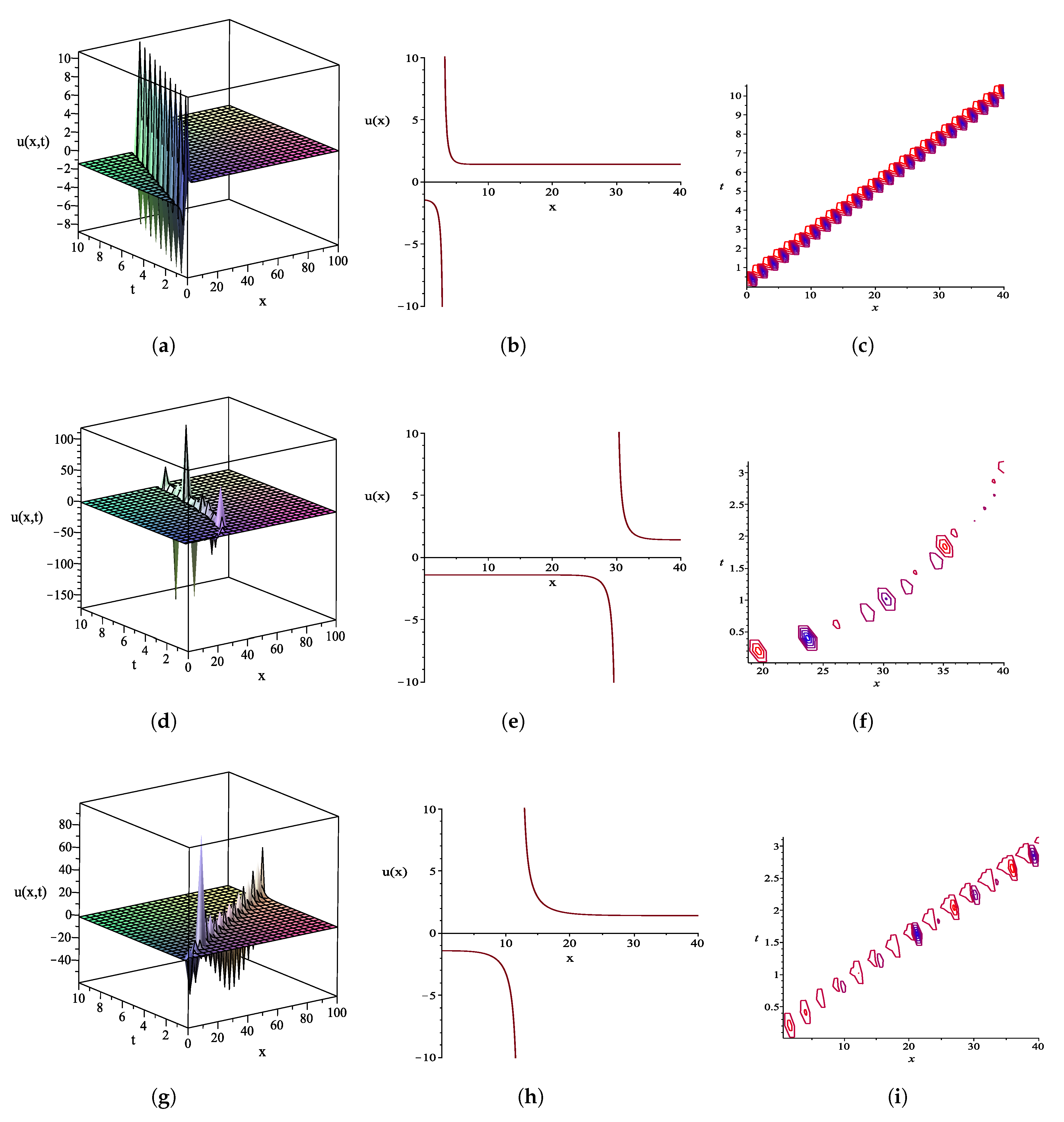
Figure 1, Figure 2 and Figure 3 demonstrate the graphical representations of some chosen exact solutions of the problem obtained using the novel -expansion method. They are described below. In Figure 1, we show different plots of the exact solution in Equation (28) using the following parameter values, , and . In particular, Figure 1a–c shows the 3-D plot, the 2-D plot with t fixed at , and the contour plot of solution (28), respectively, when the set of the fractional orders is used. Using the same parameter values as shown above except using , the 3-D graph, the 2-D graph while t is held fixed at and the contour graph of solution (28) are plotted in Figure 1d–f, respectively. Proceeding in a manner analogous to the above plots except using the fractional order set , we obtain the 3-D plot, the 2-D plot with , and the contour plot of solution (28) in Figure 1g–i, respectively. By characterizing the shapes of the plots in Figure 1, solution (28) behaves as a singular kink-type solution.
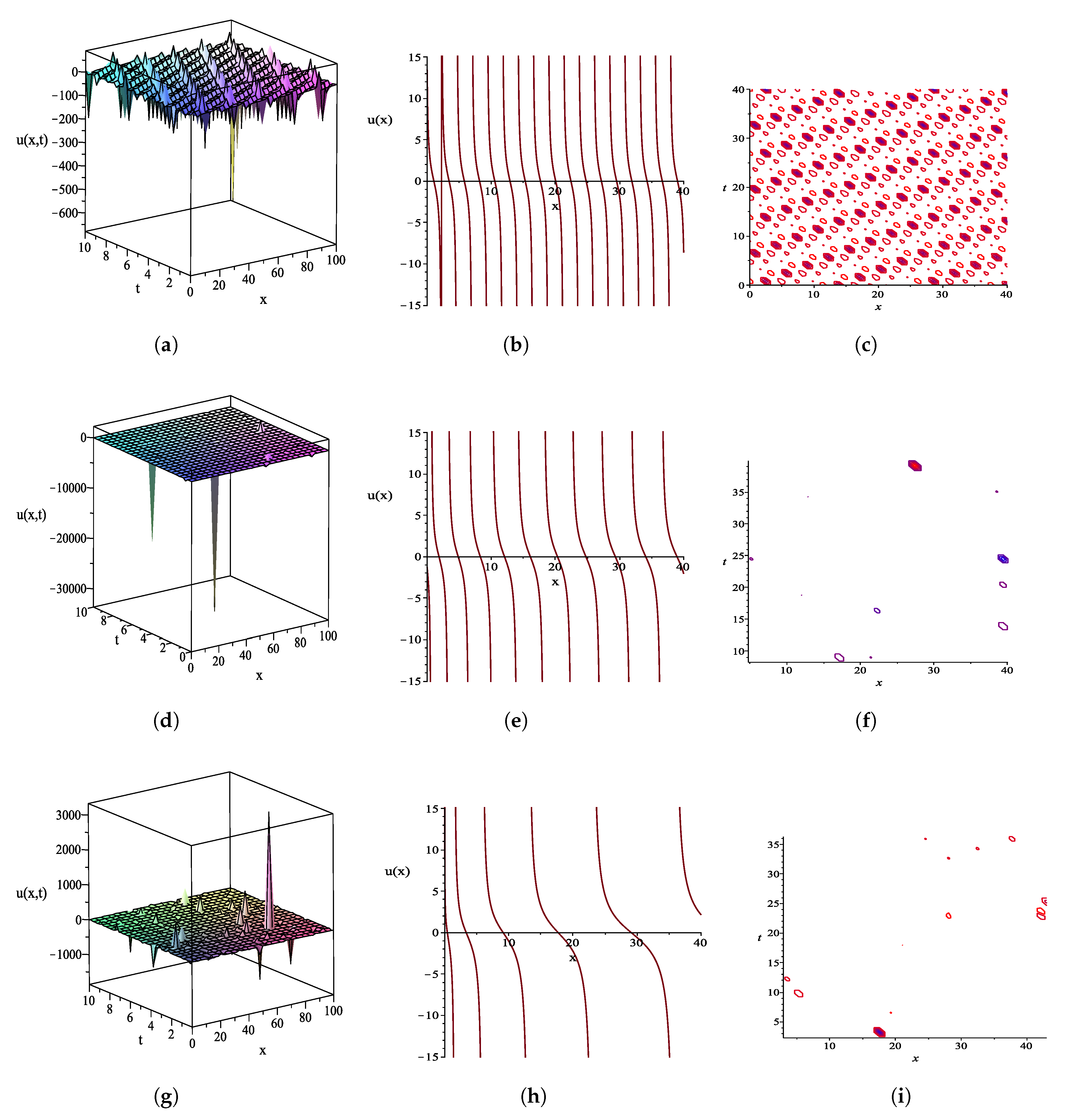
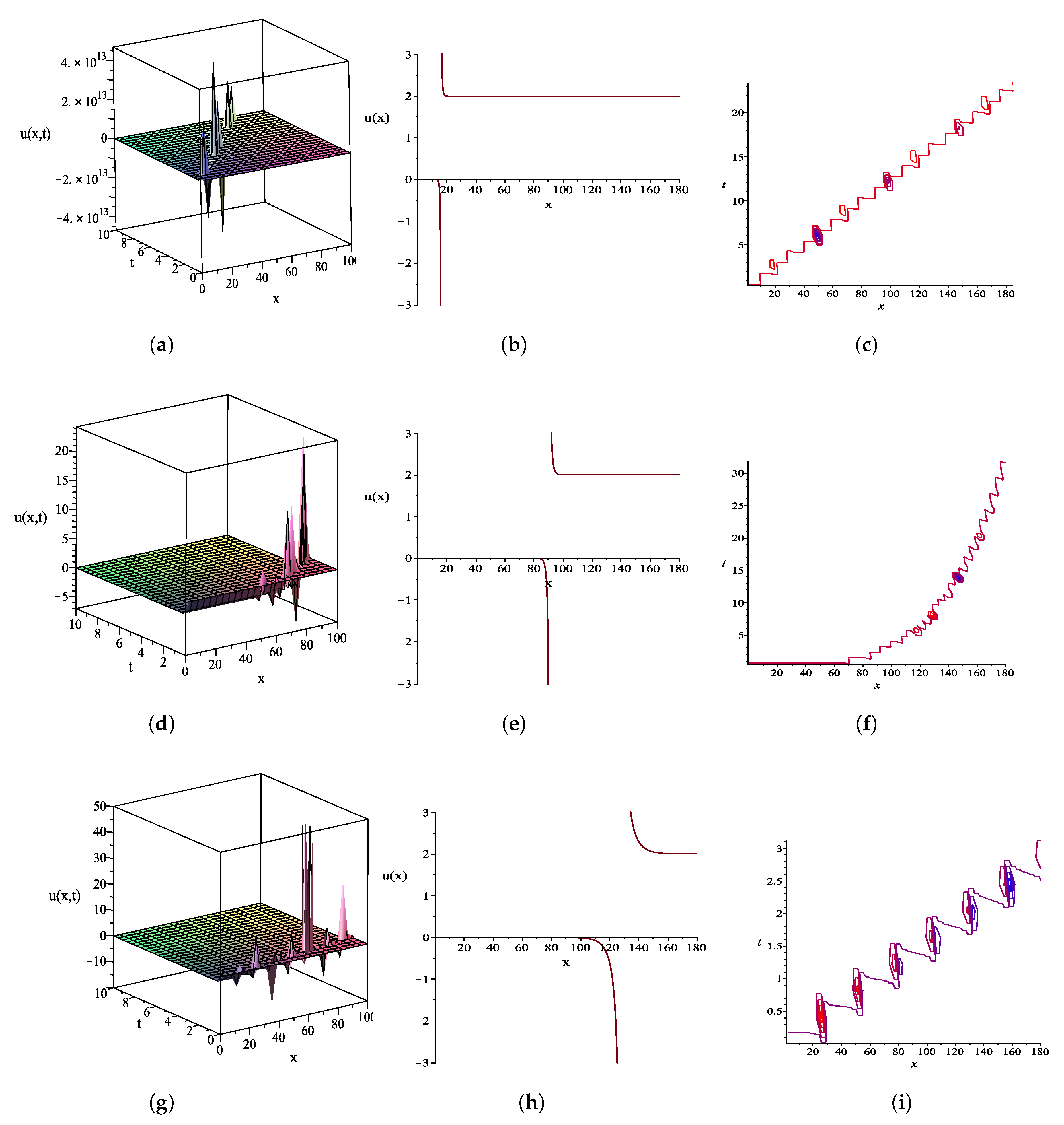
Distinct plots of the exact solution in Equation (69) are portrayed in Figure 2 using the following parameter values, , and . Specifically, Figure 2a–c describes the 3-D plot, the 2-D plot as t is fixed at , and the contour plot of solution (69), respectively, when the set of the fractional orders is used. Utilizing the same parameter values as shown above, except using , the 3-D graph, the 2-D graph when t is held fixed at , and the contour graph of solution (69) are plotted in Figure 2d–f, respectively. Proceeding in a like manner to the above plots, except using the fractional order set , we have the 3-D plot, the 2-D plot with , and the contour graph of solution (69) in Figure 2g–i, respectively. By characterizing the shapes of the plots in Figure 2, solution (69) displays the behavior of a singularly periodic traveling wave solution.
The selected exact solution in Equation (105) is plotted in Figure 3 using the three sets of the fractional orders and the following parameter values, . In particular, Figure 3a–c shows the 3-D plot, the 2-D plot when , and the contour plot of solution (105), respectively, when we use . Employing the same parameter values as shown above except using , the 3-D graph, the 2-D graph as t is held fixed at , and the contour graph of solution (105) are plotted in Figure 3d–f, respectively. Proceeding in a manner analogous to the above plots, except using the fractional order set , we obtain the 3-D plot, the 2-D plot with , and the contour graph of solution (105) in Figure 3g–i, respectively. From these plots, solution (105) is characterized as a kink-type solution.
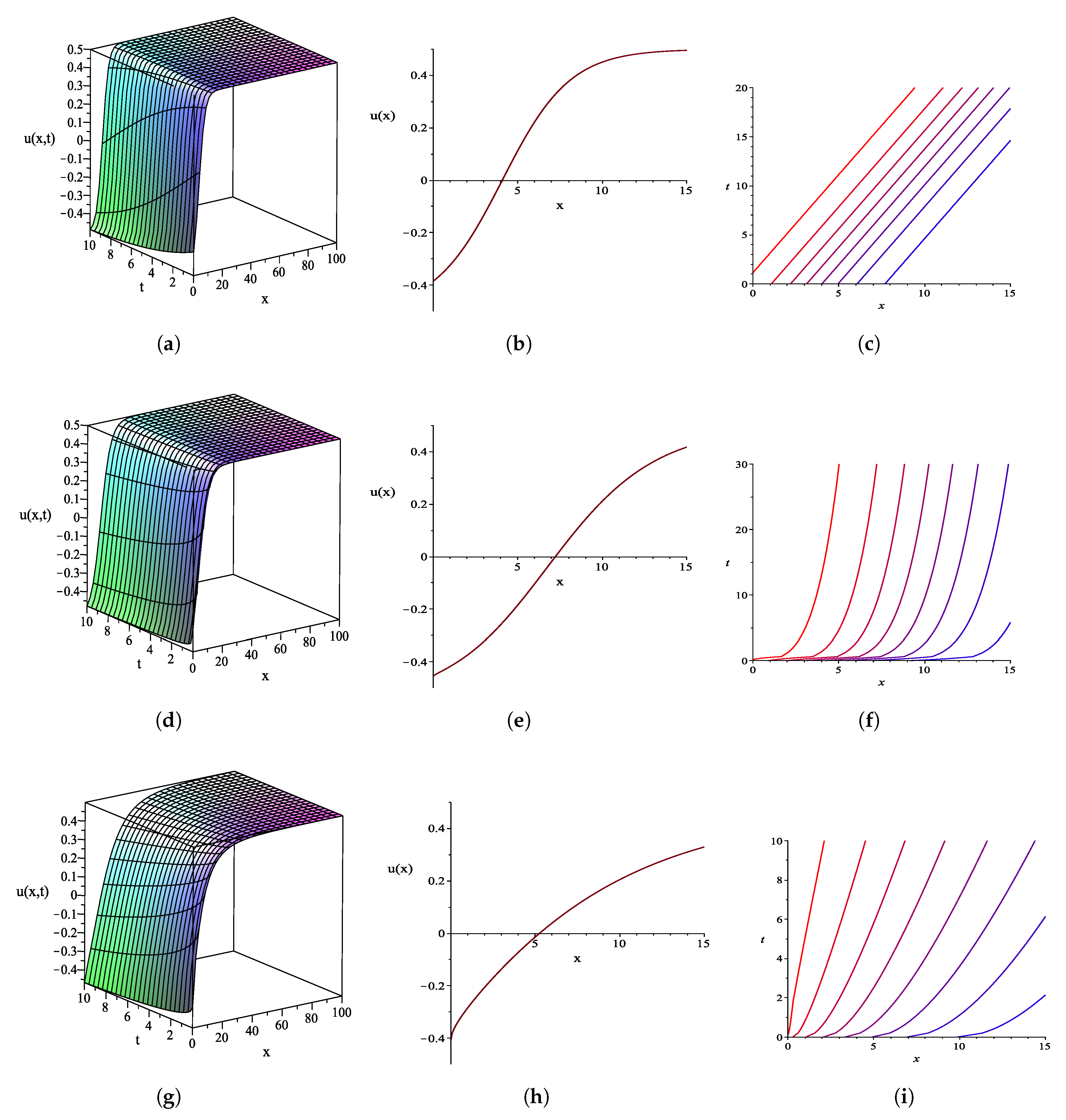
Figure 4 and Figure 5 display graphical representations of some chosen exact solutions of Equation (15) obtained using the generalized Kudryashov method. The following details graphically explain the obtained outcomes. Distinct plots of the exact solution (113) are depicted in Figure 4 using the following parameter values, . Particularly, Figure 4a–c describes the 3-D graph, the 2-D graph with , and the contour graph of solution (113), respectively, when the set of the fractional orders is employed. Using the same parameter values as mentioned above, except utilizing , the 3-D plot, the 2-D plot as t is held fixed at , and the contour plot of solution (113) are plotted in Figure 4d–f, respectively. Proceeding in like manner to the above plots, except using the fractional-order set , we have the 3-D plot, the 2-D plot with , and the contour graph of solution (113) in Figure 4g–i, respectively. By characterizing the shapes of the plots in Figure 4, solution (113) shows the behavior of a kink-type solution.
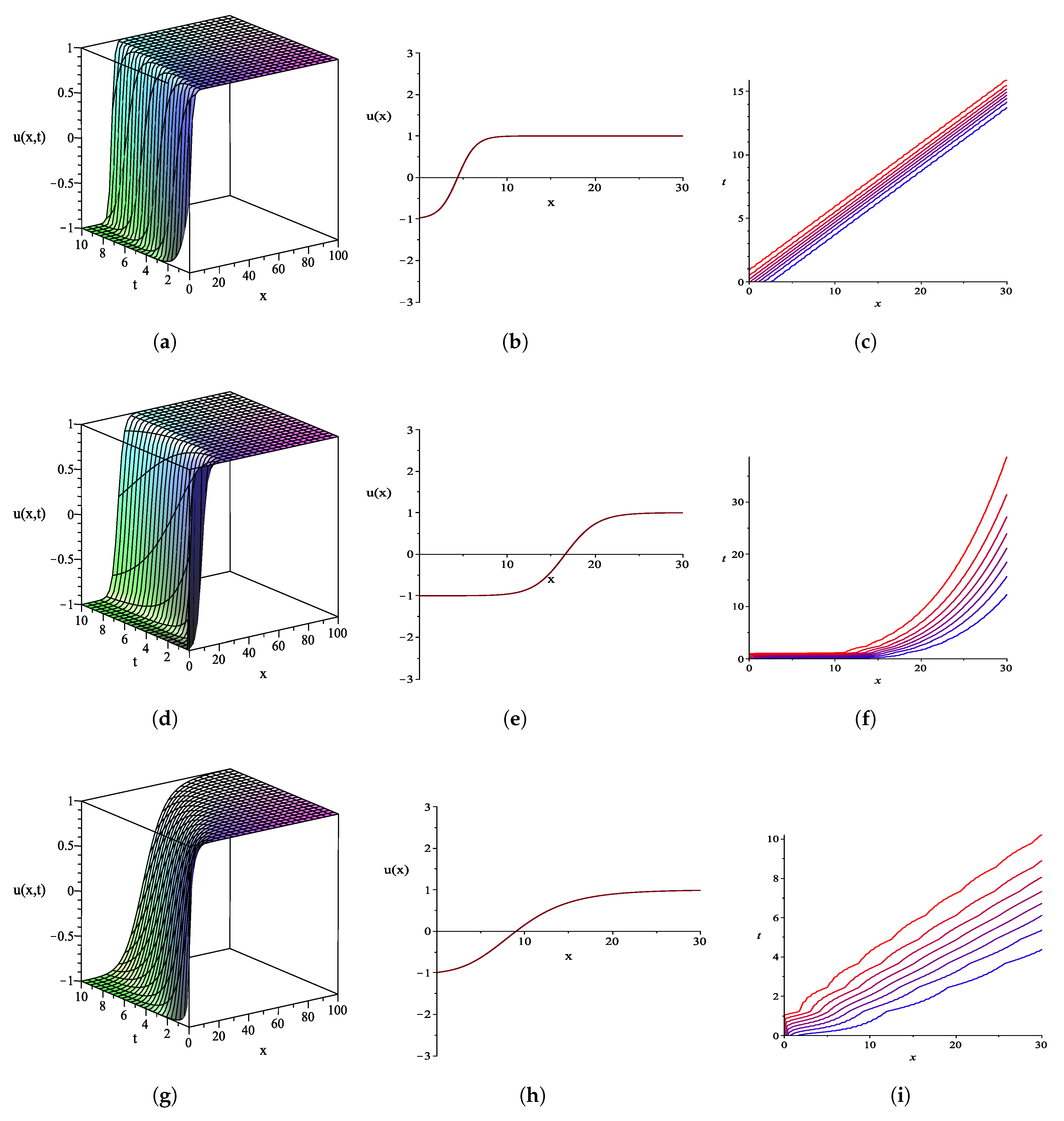
Using the second method, the exact solution in Equation (119) is graphically shown in Figure 5 with the three different sets of the fractional orders and the constant . In particular, Figure 5a–c displays the 3-D plot, the 2-D plot with , and the contour plot of solution (119), respectively, when is used. Employing the same parameter values above, except using , the 3-D graph, the 2-D graph with , and the contour graph of solution (119) are plotted in Figure 5d–f, respectively. Proceeding in a manner analogous to the previous plots, except using the fractional-order set , we obtain the 3-D plot, the 2-D plot with , and the contour graph of solution (119) in Figure 5g–i, respectively. By observing the shapes of the plots in Figure 5, solution (119) is classified into a singular multiple-soliton solution.
5. Conclusions
In this article, we have constructed explicit exact solutions of the (1+1)-dimensional conformable space-time Sharma–Tasso–Olver equation expressed in Equation (15) using the novel -expansion method and the generalized Kudryashov method with the help of the fractional complex transform and the symbolic computation package Maple 17. The obtained results have revealed that the methods are straightforward, reliable, and powerful. In particular, the novel -expansion method gives hyperbolic, trigonometric, and rational function solutions for the equation; however, the generalized Kudryashov method provides fractional solutions of the exponential functions, which are possibly converted into hyperbolic function solutions. Some of these obtained exact solutions have been graphically characterized into a variety of various physical structures such as the single-kink wave solution, the singular periodic wave solution, and the singular multiple-soliton solution. The applications of these exact solutions have been discovered in several physical phenomena such as plasma waves and optical fibers. All calculations in this investigation have been made and verified using the Maple package program. Previously, many authors had tackled the fractional Sharma–Tasso–Olver equation in different approaches. For example, finding exact solutions of the fractional Sharma–Tasso–Olver equation in the sense of the modified Riemann-Liouville derivative using the -expansion method [56], the tanh ansatz method [57], the exp method [58], the sub-equation method [59], and the improved extended tanh-coth method [13]. In addition, constructing exact solutions of the nonlinear conformable time Sharma–Tasso–Olver equation via conformable derivatives was done using the simplest equation method [60] and the direct algebraic method [61]. The Sharma–Tasso–Olver equation as shown in the above articles involves with both of only the conformable time derivative and the conformable space-time derivatives. However, in this paper, we construct exact solutions of Equation (15) in the sense of conformable derivatives with respect to x and t. To the best of our knowledge, in [62], the authors analytically solved (15) using the Exp-function method and only two exact solutions, which are expressed in terms of the exponential function solutions and characterized as kink-type solutions, were constructed. Comparing our results obtained using the novel -expansion method with the results in [62], not only the number of our exact solutions is considerably more than the number of their results, but our solutions are also classified into more different types. This is because the novel -expansion method is generalized from many similar methods such as the -expansion method, improved -expansion method, and the generalized and improved -expansion method. In consequence, some of our exact solutions of (15) via the two methods are novel and reported here for the first time. According to the mentioned advantages of the methods for obtaining exact traveling wave solutions, they could be applied efficiently for a wide range of nonlinear conformable partial differential equations or other fractional-order PDEs, which appear in several branches of the applied sciences and engineering.
Author Contributions
All authors contributed equally to the manuscript. All authors have read and agreed to the published version of the manuscript.
Funding
This research was financially supported by King Mongkut’s University of Technology North Bangkok under contract no. KMUTNB-61-KNOW-037.
Acknowledgments
The authors are grateful to anonymous referees for the valuable comments which have significantly improved this paper.
Conflicts of Interest
The authors declare no conflicts of interest.
References
- Hashim, I. Adomian decomposition method for solving BVPs for fourth-order integro-differential equations. J. Comput. Appl. Math. 2006, 193, 658–664. [Google Scholar] [CrossRef] [Green Version]
- Basak, K.C.; Ray, P.C.; Bera, R.K. Solution of non-linear Klein-Gordon equation with a quadratic non-linear term by Adomian decomposition method. Commun. Nonlinear Sci. Numer. Simul. 2009, 14, 718–723. [Google Scholar] [CrossRef]
- Gorder, R.A.V. The variational iteration method is a special case of the homotopy analysis method. Appl. Math. Lett. 2015, 45, 81–85. [Google Scholar] [CrossRef]
- Wazwaz, A. The variational iteration method: A reliable analytic tool for solving linear and nonlinear wave equations. Comput. Math. Appl. 2007, 54, 926–932. [Google Scholar] [CrossRef] [Green Version]
- Nazari, D.; Shahmorad, S. Application of the fractional differential transform method to fractional-order integro-differential equations with nonlocal boundary conditions. J. Comput. Appl. Math. 2010, 234, 883–891. [Google Scholar] [CrossRef] [Green Version]
- Bera, P.; Sil, T. Homotopy perturbation method in quantum mechanical problems. Appl. Math. Comput. 2012, 219, 3272–3278. [Google Scholar] [CrossRef]
- Nik, H.S.; Effati, S.; Shirazian, M. An approximate-analytical solution for the Hamilton-Jacobi-Bellman equation via homotopy perturbation method. Appl. Math. Model. 2012, 36, 5614–5623. [Google Scholar]
- Qin, Z.; Mu, G.; Ma, H. The ()-expansion method for the fifth-order forms of KdV-Sawada-Kotera equation. Appl. Math. Comput. 2013, 222, 29–33. [Google Scholar] [CrossRef]
- Aslan, İ. Exact solutions for fractional DDEs via auxiliary equation method coupled with the fractional complex transform. Math. Methods Appl. Sci. 2016, 39, 5619–5625. [Google Scholar] [CrossRef] [Green Version]
- Guner, O.; Bekir, A.; Ünsal, Ö. Two reliable methods for solving the time fractional Clannish Random Walkers Parabolic equation. Opt. Int. J. Light Electron Opt. 2016, 127, 9571–9577. [Google Scholar] [CrossRef]
- Abdel-Salam, E.A.B.; Gumma, E.A. Analytical solution of nonlinear space-time fractional differential equations using the improved fractional Riccati expansion method. Ain Shams Eng. J. 2015, 6, 613–620. [Google Scholar] [CrossRef] [Green Version]
- Abdel-Salam, E.A.B.; Yousif, E.A.; El-Aasser, M.A. Analytical solution of the space-time fractional nonlinear Schrödinger equation. Rep. Math. Phys. 2016, 77, 19–34. [Google Scholar] [CrossRef]
- Gómez, S.; Cesar, A. A nonlinear fractional Sharma–Tasso–Olver equation: New exact solutions. Appl. Math. Comput. 2015, 266, 385–389. [Google Scholar] [CrossRef]
- Hubert, M.B.; Betchewe, G.; Doka, S.Y.; Crepin, K.T. Soliton wave solutions for the nonlinear transmission line using the Kudryashov method and the ()-expansion method. Appl. Math. Comput. 2014, 239, 299–309. [Google Scholar] [CrossRef]
- Ryabov, P.N.; Sinelshchikov, D.I.; Kochanov, M.B. Application of the Kudryashov method for finding exact solutions of the high order nonlinear evolution equations. Appl. Math. Comput. 2011, 218, 3965–3972. [Google Scholar] [CrossRef] [Green Version]
- Mohyud-Din, S.T.; Nawaz, T.; Azhar, E.; Akbar, M.A. Fractional sub-equation method to space-time fractional Calogero-Degasperis and potential Kadomtsev-Petviashvili equations. J. Taibah Univ. Sci. 2017, 11, 258–263. [Google Scholar] [CrossRef] [Green Version]
- Abdel-Salam, E.A.; Hassan, G.F. Solutions to class of linear and nonlinear fractional differential equations. Commun. Theor. Phys. 2016, 65, 127. [Google Scholar] [CrossRef]
- Wang, M.; Li, X.; Zhang, J. The ()-expansion method and travelling wave solutions of nonlinear evolution equations in mathematical physics. Phys. Lett. A 2008, 372, 417–423. [Google Scholar] [CrossRef]
- Zhang, J.; Jiang, F.; Zhao, X. An improved ()-expansion method for solving nonlinear evolution equations. Int. J. Comput. Math. 2010, 87, 1716–1725. [Google Scholar] [CrossRef]
- Akbar, M.A.; Ali, N.H.M.; Zayed, E.M.E. A generalized and improved ()-expansion method for nonlinear evolution equations. Math. Probl. Eng. 2012, 2012, 459879. [Google Scholar] [CrossRef] [Green Version]
- Hafez, M.; Alam, M.N.; Akbar, M.A. Exact traveling wave solutions to the Klein-Gordon equation using the novel ()-expansion method. Results Phys. 2014, 4, 177–184. [Google Scholar] [CrossRef] [Green Version]
- Alam, M.N.; Akbar, M.A.; Mohyud-Din, S.T. A novel ()-expansion method and its application to the Boussinesq equation. Chin. Phys. B 2014, 23, 020203. [Google Scholar] [CrossRef]
- Alam, M.N.; Akbar, M.A. Traveling wave solutions of the nonlinear (1+1)-dimensional modified Benjamin-Bona-Mahony equation by using novel ()-expansion method. Phys. Rev. Res. Int. 2014, 4, 147–165. [Google Scholar]
- Hafez, M.G.; Zheng, B.; Akbar, M. Exact travelling wave solutions of the coupled nonlinear evolution equation via the Maccari system using novel ()-expansion method. Egypt. J. Basic Appl. Sci. 2015, 2, 206–220. [Google Scholar] [CrossRef] [Green Version]
- Alam, M.N.; Belgacem, F.B.M.; Akbar, M.A. Analytical Treatment of the Evolutionary (1+ 1)-Dimensional Combined KdV-mKdV Equation via the Novel ()-Expansion Method. J. Appl. Math. Phys. 2015, 3, 1571. [Google Scholar] [CrossRef] [Green Version]
- Alam, M.N.; Hafez, M.; Belgacem, F.B.M.; Akbar, M.A. Applications of the novel ()-expansion method to find new exact traveling wave solutions of the nonlinear coupled Hsiggs field equation. Nonlinear Stud. 2015, 22, 613–633. [Google Scholar]
- Hafez, M. New travelling wave solutions of the (1+1)-dimensional cubic nonlinear Schrödinger equation using novel ()-expansion method. Beni-Suef Univ. J. Basic Appl. Sci. 2016, 5, 109–118. [Google Scholar] [CrossRef] [Green Version]
- Alam, M.N.; Belgacem, F.B.M. Exact Traveling Wave Solutions for the (1+ 1)-Dimensional Compound KdVB Equation via the Novel ()-Expansion Method. Int. J. Mod. Nonlinear Theory Appl. 2016, 5, 28. [Google Scholar] [CrossRef] [Green Version]
- Akbar, M.A.; Alam, M.N.; Hafez, M.G. Application of the novel ()-expansion method to construct traveling wave solutions to the positive Gardner–KP equation. Indian J. Pure Appl. Math. 2016, 47, 85–96. [Google Scholar] [CrossRef]
- Islam, M.S.; Khan, K.; Arnous, A.H. Generalized Kudryashov method for solving some (3+ 1)-dimensional nonlinear evolution equations. New Trends Math. Sci. 2015, 3, 46. [Google Scholar]
- Kaplan, M.; Bekir, A.; Akbulut, A. A generalized Kudryashov method to some nonlinear evolution equations in mathematical physics. Nonlinear Dyn. 2016, 85, 2843–2850. [Google Scholar] [CrossRef]
- Mahmud, F.; Samsuzzoha, M.; Akbar, M.A. The generalized Kudryashov method to obtain exact traveling wave solutions of the PHI-four equation and the Fisher equation. Results Phys. 2017, 7, 4296–4302. [Google Scholar] [CrossRef]
- Biswas, A.; Sonmezoglu, A.; Ekici, M.; Mirzazadeh, M.; Zhou, Q.; Moshokoa, S.P.; Belic, M. Optical soliton perturbation with fractional temporal evolution by generalized Kudryashov’s method. Optik 2018, 164, 303–310. [Google Scholar] [CrossRef]
- Nestor, S.; Justin, M.; Douvagai; Betchewe, G.; Doka, S.Y.; Kofane, T. New Jacobi elliptic solutions and other solutions with quadratic–Cubic nonlinearity using two mathematical methods. Asian-Eur. J. Math. 2018, 13, 2050043. [Google Scholar] [CrossRef]
- Houwe, A.; Justin, M.; Doka, S.Y.; Crepin, K.T. New traveling wave solutions of the perturbed nonlinear Schrödingers equation in the left–handed metamaterials. Asian-Eur. J. Math. 2018, 13, 2050022. [Google Scholar] [CrossRef]
- Lu, D.; Seadawy, A.R.; Khater, M.M. Structure of solitary wave solutions of the nonlinear complex fractional generalized Zakharov dynamical system. Adv. Differ. Equ. 2018, 2018, 266. [Google Scholar] [CrossRef] [Green Version]
- Demiray, S.T.; Bulut, H. Soliton solutions of some nonlinear evolution problems by GKM. Neural Comput. Appl. 2019, 31, 287–294. [Google Scholar] [CrossRef]
- Habib, M.; Ali, H.S.; Miah, M.M.; Akbar, M.A. The generalized Kudryashov method for new closed form traveling wave solutions to some NLEEs. AIMS Math. 2019, 4, 896. [Google Scholar] [CrossRef]
- Wazwaz, A.M. New solitons and kinks solutions to the Sharma-Tasso-Olver equation. Appl. Math. Comput. 2007, 188, 1205–1213. [Google Scholar] [CrossRef]
- Pan, J.T.; Chen, W.Z. A new auxiliary equation method and its application to the Sharma-Tasso-Olver model. Phys. Lett. A 2009, 373, 3118–3121. [Google Scholar]
- Bekir, A.; Boz, A. Exact solutions for nonlinear evolution equations using Exp-function method. Phys. Lett. A 2008, 372, 1619–1625. [Google Scholar] [CrossRef]
- He, Y.; Li, S.; Long, Y. Exact solutions to the Sharma-Tasso-Olver equation by using improved ()-expansion method. J. Appl. Math. 2013, 2013, 247234. [Google Scholar] [CrossRef] [Green Version]
- Uğurlu, Y.; Kaya, D. Analytic method for solitary solutions of some partial differential equations. Phys. Lett. A 2007, 370, 251–259. [Google Scholar] [CrossRef]
- Khalil, R.; Horani, M.A.; Yousef, A.; Sababheh, M. A new definition of fractional derivative. J. Comput. Appl. Math. 2014, 264, 65–70. [Google Scholar] [CrossRef]
- Kumar, D.; Seadawy, A.R.; Joardar, A.K. Modified Kudryashov method via new exact solutions for some conformable fractional differential equations arising in mathematical biology. Chin. J. Phys. 2018, 56, 75–85. [Google Scholar] [CrossRef]
- Rezazadeh, H.; Korkmaz, A.; Eslami, M.; Vahidi, J.; Asghari, R. Traveling wave solution of conformable fractional generalized reaction Duffing model by generalized projective Riccati equation method. Opt. Quantum Electron. 2018, 50, 150. [Google Scholar] [CrossRef]
- Korkmaz, A. Explicit exact solutions to some one-dimensional conformable time fractional equations. Waves Random Complex Media 2019, 29, 124–137. [Google Scholar] [CrossRef]
- Ekici, M.; Mirzazadeh, M.; Eslami, M.; Zhou, Q.; Moshokoa, S.P.; Biswas, A.; Belic, M. Optical soliton perturbation with fractional-temporal evolution by first integral method with conformable fractional derivatives. Optik 2016, 127, 10659–10669. [Google Scholar] [CrossRef]
- Tarasov, V.E. No nonlocality. No fractional derivative. Commun. Nonlinear Sci. Numer. Simul. 2018, 62, 157–163. [Google Scholar] [CrossRef] [Green Version]
- He, J.H.; Elagan, S.; Li, Z. Geometrical explanation of the fractional complex transform and derivative chain rule for fractional calculus. Phys. Lett. A 2012, 376, 257–259. [Google Scholar] [CrossRef]
- Su, W.H.; Yang, X.J.; Jafari, H.; Baleanu, D. Fractional complex transform method for wave equations on Cantor sets within local fractional differential operator. Adv. Differ. Equ. 2013, 2013, 97. [Google Scholar] [CrossRef] [Green Version]
- Güner, O.; Bekir, A.; Cevikel, A.C. A variety of exact solutions for the time fractional Cahn–Allen equation. Eur. Phys. J. Plus 2015, 130, 146. [Google Scholar] [CrossRef]
- Sirisubtawee, S.; Koonprasert, S.; Khaopant, C.; Porka, W. Two Reliable Methods for Solving the (3 + 1)-Dimensional Space-Time Fractional Jimbo-Miwa Equation. Math. Probl. Eng. 2017, 2017, 1–30. [Google Scholar] [CrossRef] [Green Version]
- Zhu, S.D. The generalizing Riccati equation mapping method in non-linear evolution equation: Application to (2+1)-dimensional Boiti-Leon-Pempinelle equation. Chaos Solitons Fractals 2008, 37, 1335–1342. [Google Scholar]
- Zheng, C.L. Comments on “The generalizing Riccati equation mapping method in nonlinear evolution equation: Application to (2 + 1)-dimensional Boiti-Leon-Pempinelle equation”. Chaos Solitons Fractals 2009, 39, 1493–1495. [Google Scholar] [CrossRef]
- Uddin, M.H.; Khan, M.A.; Akbar, M.A.; Haque, M.A. Multi-solitary wave solutions to the general time fractional Sharma–Tasso–Olver equation and the time fractional Cahn–Allen equation. Arab. J. Basic Appl. Sci. 2019, 26, 193–201. [Google Scholar] [CrossRef]
- Guner, O.; Korkmaz, A.; Bekir, A. Dark soliton solutions of space-time fractional Sharma–Tasso–Olver and potential Kadomtsev–Petviashvili equations. Commun. Theor. Phys. 2017, 67, 182. [Google Scholar] [CrossRef]
- Kaplan, M.; Bekir, A. A novel analytical method for time-fractional differential equations. Optik 2016, 127, 8209–8214. [Google Scholar] [CrossRef]
- Jafari, H.; Tajadodi, H.; Baleanu, D.; Al-Zahrani, A.; Alhamed, Y.; Zahid, A. Fractional sub-equation method for the fractional generalized reaction Duffing model and nonlinear fractional Sharma-Tasso-Olver equation. Open Phys. 2013, 11, 1482–1486. [Google Scholar] [CrossRef]
- Chen, C.; Jiang, Y.L. Simplest equation method for some time-fractional partial differential equations with conformable derivative. Comput. Math. Appl. 2018, 75, 2978–2988. [Google Scholar] [CrossRef]
- Rezazadeh, H.; Khodadad, F.S.; Manafian, J. New structure for exact solutions of nonlinear time fractional Sharma–Tasso–Olver equation via conformable fractional derivative. Appl. Appl. Math. Int. J. 2017, 12, 13–21. [Google Scholar]
- Yaslan, H.Ç.; Girgin, A. Exp-function method for the conformable space-time fractional STO, ZKBBM and coupled Boussinesq equations. Arab. J. Basic Appl. Sci. 2019, 26, 163–170. [Google Scholar] [CrossRef] [Green Version]
Figure 1.
Associated plots of in Equation (28): (a–c) 3-D plot, 2-D plot, and contour plot, respectively, when ; (d–f) 3-D plot, 2-D plot, and contour plot, respectively, when ; (g–i) 3-D plot, 2-D plot, and contour plot, respectively, when .
Figure 1.
Associated plots of in Equation (28): (a–c) 3-D plot, 2-D plot, and contour plot, respectively, when ; (d–f) 3-D plot, 2-D plot, and contour plot, respectively, when ; (g–i) 3-D plot, 2-D plot, and contour plot, respectively, when .

Figure 2.
Associated plots of in Equation (69): (a–c) 3-D plot, 2-D plot, and contour plot, respectively, when ; (d–f) 3-D plot, 2-D plot, and contour plot, respectively, when ; (g–i) 3-D plot, 2-D plot, and contour plot, respectively, when .
Figure 2.
Associated plots of in Equation (69): (a–c) 3-D plot, 2-D plot, and contour plot, respectively, when ; (d–f) 3-D plot, 2-D plot, and contour plot, respectively, when ; (g–i) 3-D plot, 2-D plot, and contour plot, respectively, when .

Figure 3.
Associated plots of in Equation (105): (a–c) 3-D plot, 2-D plot, and contour plot, respectively, when ; (d–f) 3-D plot, 2-D plot, and contour plot, respectively, when ; (g–i) 3-D plot, 2-D plot, and contour plot, respectively, when .
Figure 3.
Associated plots of in Equation (105): (a–c) 3-D plot, 2-D plot, and contour plot, respectively, when ; (d–f) 3-D plot, 2-D plot, and contour plot, respectively, when ; (g–i) 3-D plot, 2-D plot, and contour plot, respectively, when .

Figure 4.
Associated plots of u(x, t) in Equation (113): (a–c) 3-D plot, 2-D plot, and contour plot, respectively, when ; (d–f) 3-D plot, 2-D plot, and contour plot, respectively, when ; (g–i) 3-D plot, 2-D plot, and contour plot, respectively, when .
Figure 4.
Associated plots of u(x, t) in Equation (113): (a–c) 3-D plot, 2-D plot, and contour plot, respectively, when ; (d–f) 3-D plot, 2-D plot, and contour plot, respectively, when ; (g–i) 3-D plot, 2-D plot, and contour plot, respectively, when .

Figure 5.
Associated plots of u(x, t) in Equation (119): (a–c) 3-D plot, 2-D plot, and contour plot, respectively, when {}; (d–f) 3-D plot, 2-D plot, and contour plot, respectively, when {}; (g–i) 3-D plot, 2-D plot, and contour plot, respectively, when .
Figure 5.
Associated plots of u(x, t) in Equation (119): (a–c) 3-D plot, 2-D plot, and contour plot, respectively, when {}; (d–f) 3-D plot, 2-D plot, and contour plot, respectively, when {}; (g–i) 3-D plot, 2-D plot, and contour plot, respectively, when .

© 2020 by the authors. Licensee MDPI, Basel, Switzerland. This article is an open access article distributed under the terms and conditions of the Creative Commons Attribution (CC BY) license (http://creativecommons.org/licenses/by/4.0/).
Share and Cite
MDPI and ACS Style
Sirisubtawee, S.; Koonprasert, S.; Sungnul, S. New Exact Solutions of the Conformable Space-Time Sharma–Tasso–Olver Equation Using Two Reliable Methods. Symmetry 2020, 12, 644. https://0-doi-org.brum.beds.ac.uk/10.3390/sym12040644
AMA Style
Sirisubtawee S, Koonprasert S, Sungnul S. New Exact Solutions of the Conformable Space-Time Sharma–Tasso–Olver Equation Using Two Reliable Methods. Symmetry. 2020; 12(4):644. https://0-doi-org.brum.beds.ac.uk/10.3390/sym12040644
Chicago/Turabian StyleSirisubtawee, Sekson, Sanoe Koonprasert, and Surattana Sungnul. 2020. "New Exact Solutions of the Conformable Space-Time Sharma–Tasso–Olver Equation Using Two Reliable Methods" Symmetry 12, no. 4: 644. https://0-doi-org.brum.beds.ac.uk/10.3390/sym12040644
Note that from the first issue of 2016, this journal uses article numbers instead of page numbers. See further details here.