Automatic Segmentation and Measurement of Infantile Hemangioma

Abstract

Infantile hemangiomas (IHs) are a type of vascular tumors that affect around 10% of newborns. The measurement of the lesion size and the assessment of the evolution is done manually by the physician. This paper presents an algorithm for the automatic computation of the IH lesion surface. The image scale is computed by using the Hough transform and the total variation. As pre-processing, a geometric correction step is included, which ensures that the lesions are viewed as perpendicular to the camera. The image segmentation is based on K-means clustering applied on a five-plane image; the five planes being selected from seven planes with the use of the Karhunen-Loeve transform. Two of the seven planes are 2D total variation filters, based on symmetrical kernels, designed to highlight the IH specific texture. The segmentation performance was assessed on 30 images, and a mean border error of 9.31% was obtained.

1. Introduction

Infantile hemangiomas (IHs) represent a type of vascular tumor that has an incidence of 3% to 10% in newborns [1,2]. Usually, they appear and start to develop rapidly around the first two to five months of life and then have a natural slow involution in the following years [3]. Their shape and size are very different from subject to subject; some hemangiomas may become function-threatening, and that is why a precise method of measurement and prediction of evolution is needed. Usually, the IH size assessment is manually performed by the physician by using a measuring tape. However, this method of measurement is imprecise (it usually implies recording height and width, without any information about the geometry), due to the irregular shapes of the hemangiomas, and from this comes the motivation to develop an automatic measurement of the IH surface.

In biomedical image analysis, the automatic measurement of a lesion relies on image segmentation techniques. Image segmentation consists of partitioning the image into regions (called classes or subsets) [4] which are homogenous in terms of some features (color, texture, gray level, etc.). There is a wide variety of segmentation methods [4,5], but there is no standard technique that works well for all medical image categories. Usually, medical images contain some uncertainty concerning the border of some lesions or organs, uncertainty produced by the image acquisition or reconstruction process, and this uncertainty makes the segmentation task more difficult [5].

There are only a few image processing and analysis papers addressing the problem of assessment of the size of IHs and the prediction of their evolution. The first paper was the one by Zambanini et al. [6]. Thus, in [6], IH lesion segmentation was performed using a perceptron on four features (G from RGB, H from HSV, a* from L*a*b*, and a feature representing the distance between the a*b* values of a pixel and the normalized corresponding values of the skin). The image scale was automatically computed by extracting the marks on a ruler placed near the lesion, by global thresholding. The authors also performed image registration and a detection of hemangioma regression.

The authors of [7] used a two-level thresholding segmentation on the a* channel from L*a*b*, and in [8] a color constancy approach was applied to correct the variation of colors due to different illumination. They reported a detection rate of 85% and a false positives rate of 16.4%.

In [9], the L*a*b* color space was proven to be the optimal color space for image segmentation, chosen among five different color spaces; then, a MAP-Markov segmentation was implemented, with an automatic learning step. The reported border error was 19.49%.

The performances of three segmentation methods (Otsu, fuzzy C-means (FCM), and a region growing algorithm based on FCM, RG-FCM) were compared in [10]; the best result, 91.51%, was obtained with RG-FCM. In [11] the image was segmented in 25 classes using a self-organizing map (SOM) network, and then the number of classes was reduced to only two classes (hemangioma and non-hemangioma) with a morphological approach. On average, they obtained a 1.06% increase in performance compared to when they used FCM.

The authors of [12] tested five classic segmentation methods (Otsu, Canny, FCM, GVF snakes, and Shortest path) and two different convolutional neural network architectures, a standard linear CNN and a two-inputs DAG topology. The best results were obtained with the shortest path method and the two-inputs CNN. More recently, in [13], a crop-based classifier based on a standard linear convolutional neural network was proposed; the classifier receives small 64 × 64 RGB image patches and returns two classes: hemangioma and non-hemangioma; the maximum obtained accuracy is 93.84%.

The Novelty of This Paper

In [14] we proposed an automatic measurement of the hemangioma lesion from digital photographs containing a ruler. The shape and size of the hemangioma lesion depends on the viewing angle and the distance to the camera, and this makes the evaluation of the lesion evolution in time impractical.

In this paper we expand the work presented in [14] by adding some additional steps, which ensure that the photographs are geometrically transformed in such a way that they appear as taken from the same distance to the camera, and that the camera is perpendicular to the lesion. This step is necessary to ensure the correct assessment of the lesion shape and size for an accurate subsequent evolution follow up. The segmentation algorithm was also improved by eliminating some programming errors, performing some optimizations, adding some additional features, and adding automatic selection of the most significative image planes for the segmentation with the use of the Karhunen-Loeve transform. Seven image planes were used for segmentation (including a new defined total variation filter), instead of only four in [14]. The segmentation accuracy was assessed in terms of border error, by using some manually segmented images (ground truth). An improvement of at least 5% compared to that of the previous work was obtained.

This paper is organized as follows. In Section 2, we present the proposed algorithm, in Section 3 we show the obtained experimental results, and in Section 4 we discuss the conclusions.

2. Materials and Methods

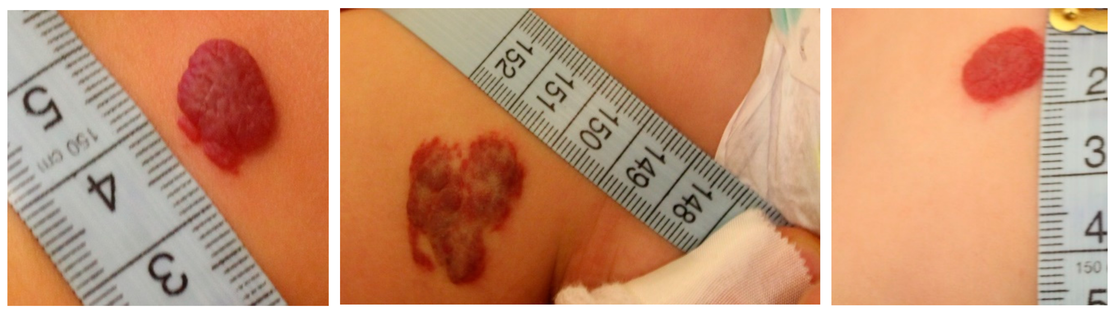
For this study we used a database of 30 RGB images (at a resolution of about 1300 × 1200 pixels) obtained from the Marie Curie children’s hospital in Bucharest. The images were acquired during the project mentioned in the acknowledgements section, and their use for research was approved by the hospital. Each image contains a hemangioma lesion (located on different parts of the body such as chest, legs, face, etc.), and was acquired using different cameras and in different illumination conditions. For measurement purposes, a ruler was placed near each lesion. In Figure 1, some images from the database are shown.

The proposed algorithm contains the following steps:

• Automatic computation of the image scale and the detection of the ruler direction line.
• Rotation of the image such that the ruler becomes vertical.
• Extraction of the centimeter area.
• Extraction of the digits from the centimeter area.
• Performance of optical character recognition (OCR) of each of the objects that could be a digit. We search for the digits: 2–9.
• Geometric transformation of the entire image such that the detected digit is geometrically aligned to its corresponding frontal template.
• Segmentation of the hemangioma.
• Computation of the lesion surface.

2.1. Detection of the Ruler and Computation of the Image Scale

For the detection of the ruler within the image, we developed the following algorithm:

-

Find the edges, using the Canny method;

-

Apply the Hough transform for lines on the edges of the image (obtained in the previous step), and keep only the lines that are at least 250 pixels long (the minimum length of 250 pixels was selected because it corresponds to around 1 cm length on the ruler at the resolution at which the images were acquired; if a smaller value is chosen, the algorithm still works, but the processing time increases due to the detection of more lines within the image);

-

For each extracted line, record the 1D intensity profile along the line and compute its total variation (1);

-

The line which has the maximum total variation is selected;

-

Detect the peaks from the intensity profile of the line and then compute the median distance between two consecutive peaks.

The total variation of the function is computed by:

$$v={\displaystyle \sum _{k=2}^N\left|f(k)-f(k-1)\right|}$$

(1)

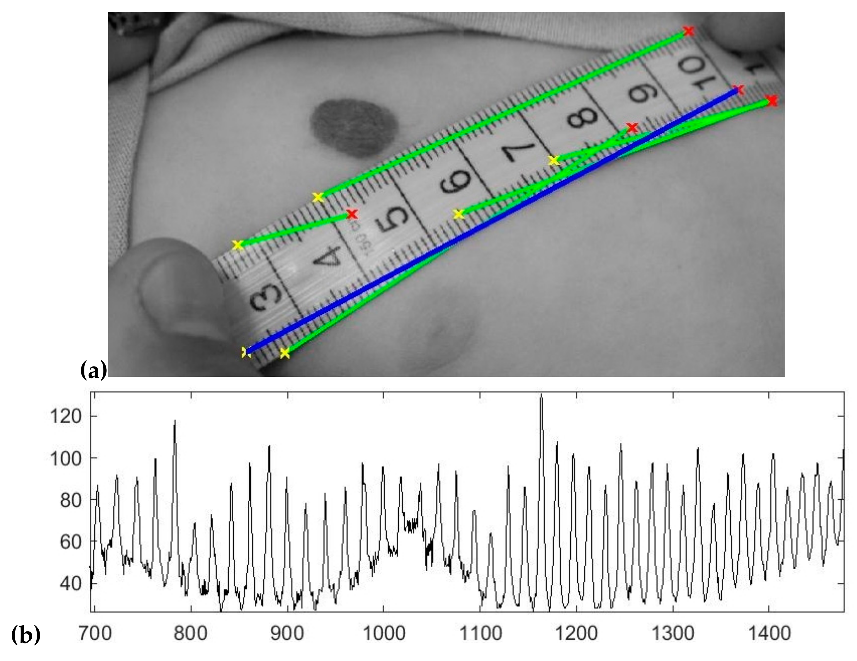
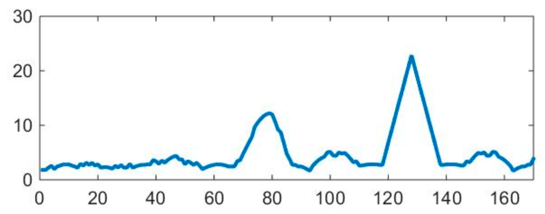
where f is the intensity profile of the line, N represents the number of pixels, and k is the index of each pixel. From all the lines detected in the image, the one which has the maximum v is selected (this line will contain most of the mm gradations from the ruler). An example of lines detected within the image using the Hough transform is shown in Figure 2a; the line with the maximum total variation is colored in blue. In Figure 2b, one can see the peaks, which correspond to the mm gradations of the ruler, from the 1D intensity “signal” along the selected line. All the lines that are at least 250 pixels long come from the mm gradations on the sides of the ruler, gradations that are aligned, hence they give a strong response in the accumulator space of the Hough transform. In addition, with the Hough transform being applied on the edges of the image (which is a binary image that contains white pixels only on contour areas) it is impossible that a line longer than 250 pixels appears elsewhere than along the mm gradations.

After computing the median distance between two consecutive gradations on the ruler, one can compute the area of a pixel in mm² with the formula: pixel area = 1/(d * d), where d is the above-mentioned distance.

After the detection of the ruler, one knows its direction from the Hough transform, and we apply an image rotation so that the ruler becomes vertical. This step is necessary for the OCR to work. The rotation is performed using a classic rotation matrix, with the output image being augmented to contain the rotated image; the nearest neighbor approach was used for the interpolation of the output pixels.

The extraction of the ruler area is then performed based on the hypothesis that the region’s color is a certain shade of gray (if the difference between the minimum and maximum value from the RGB triplet is smaller than a threshold, the pixel is considered as a shade of gray), and it includes at least a part of the line retained above. The ruler is gray within all the images.

Then, in order to extract the digits from the ruler, a K-means algorithm with two classes is applied on the ruler region. The class which represents the digits is automatically chosen by considering the number of pixels within each of the two regions (the background region of the ruler is much larger than the area covered by digits within the ruler). Then, a labeling step is performed only on the regions that are potential digit candidates, and only the compact regions that are of the size of a digit are retained. The thresholds for digit size are automatically computed using the image scale obtained in the ruler-detection step.

Once the digits have been extracted, they are recognized by a standard OCR algorithm. We used the current OCR implementation from Matlab, which is an open-source OCR, more precisely the Tesseract OCR engine [15]. We used the character confidence measure provided by the OCR to discern if the extracted objects are digits or noise. In our implementation, we used digits from 2 to 9 to implement the geometric transformation. For most of the images, the beginning of the ruler—around digits 2 to 4—is placed near the lesion. For the images where the digit 1 is the closest to the lesion (2 images), we decided that this digit is not wide enough to be used for a geometric transformation (errors due to noise are significant for digit 1).

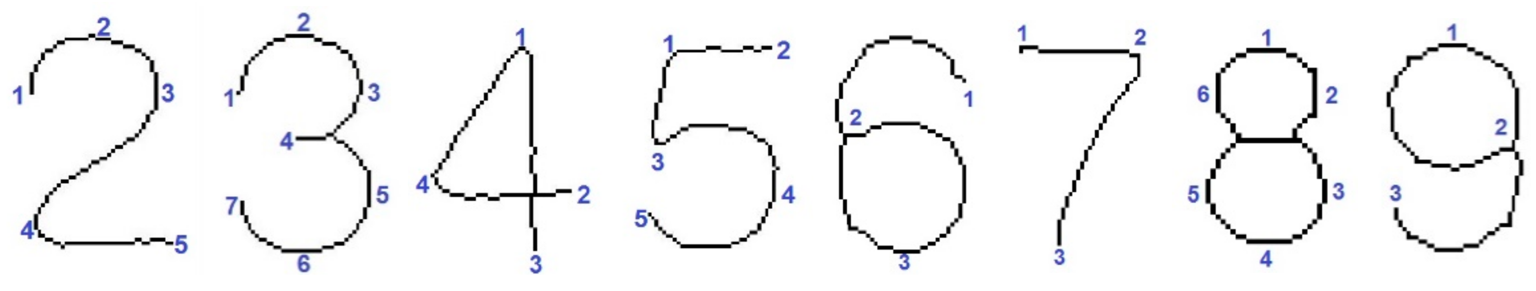
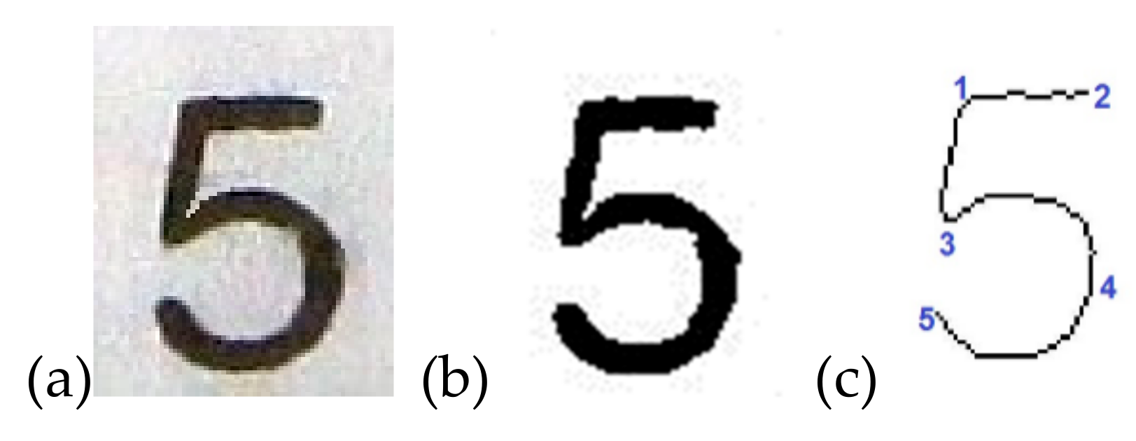
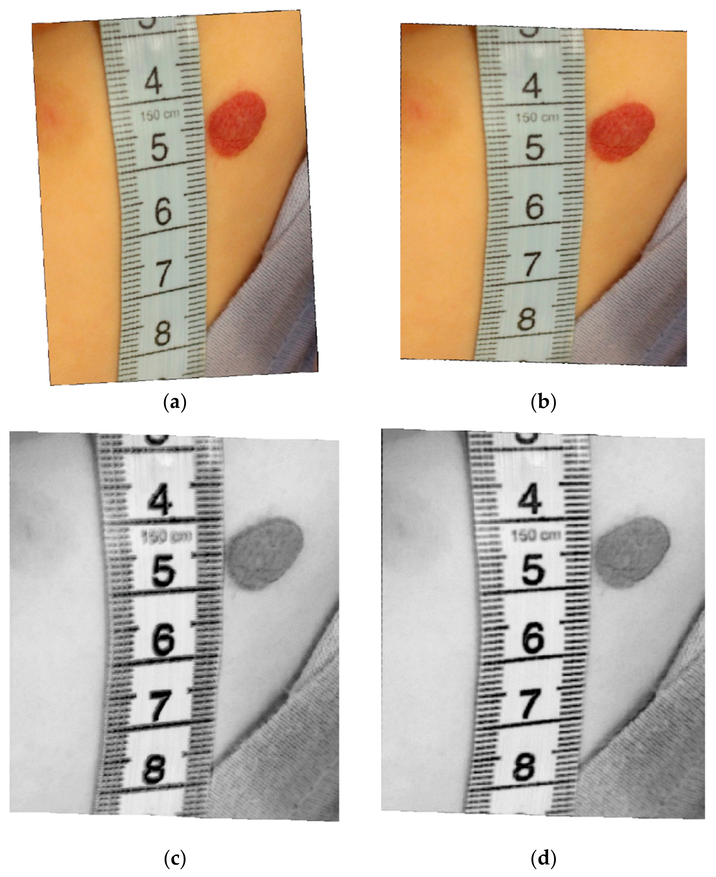
For the affine type of transformation, a minimum of three key points is required. For each digit, one defines at least three key points, as one can see in Figure 3. The choice of each key point is customized for each digit (the location and the number of key points are fixed for each digit, i.e., all number 2s are identified with 5 key points, all number 3s with 7 key points etc.). To determine the key points in each of the detected digits, one binarizes the image (Figure 4b), then one extracts a skeletonized shape of the digit by applying a geometric skeletonization algorithm. Afterwards, the key points are detected by analyzing the local curvature of the skeletonized shape.

Figure 5 presents the curvature determined along the contour line of the digit five. The two maximum curvature peaks are used to set the key points 1 and 3; the key points 5 and 2 are termination points, and 4 is at half-distance from 3 to 5.

The geometric transformation matrix is determined by solving a system of equations like the one in (2), with at least 6 unknowns if one has a minimum set of three key points pairs, by optimization in the sense of mean square error. Once the coordinates of key points are detected on the processed digit, a geometrical affine transform is then computed to render the digit in an ideal, frontal view (photographed perpendicularly to the camera). To this end, the spatial coordinates of the same key points from the ideal view are used to compute the six optimal parameters (a₁₁, a₁₂, a₂₁, a₂₂, b₁, b₂) of the transform in Equation (2), that best fit (in the mean-squared error sense) the set of original coordinates of key-points to the set of coordinates of ideal key points.

$$\left[\begin{array}{l}{x}_{t_i}\\ y_{t_i}\end{array}\right]=\left[\begin{array}{cc}{a}_{11}& a_{12}\\ a_{21}& a_{22}\end{array}\right]\left[\begin{array}{l}{x}_{s_i}\\ y_{s_i}\end{array}\right]+\left[\begin{array}{c}{b}_1\\ b_2\end{array}\right]$$

(2)

In Equation (2), [x_ti, y_ti] represent the target (ideal) coordinates of key point #i, whereas [x_si, y_si] represent the original coordinates of the same key point. Thus, the deformed digit will be transformed in an “ideally” photographed digit. We then apply this geometrical transformation matrix to the whole image.

For the geometric transformation, from the digits detected by the OCR, we chose the one that is the closest to the lesion. For this, we used the “learning image” described in [9]. This image contains a set of points (much smaller than the entire hemangioma), chosen very restrictively, which certainly belong to the lesion. These points are determined in the following manner:

• Apply a Canny edge detection on the original image.
• Build an edge density image, D, by convolving the contour map with a blurring kernel.
• Construct a binary image B, which contains the higher edge density, by thresholding D with an adaptive threshold (set at 45% of the higher contour density).
• Keep the pixels from B that have a red component (from RGB) 55% higher than the green component and 55% higher than the blue one.

We tested the above described method on all the images from the database, and the detected set of points always belonged to the lesion.

2.2. Hemangioma Lesion Segmentation

The segmentation of the hemangioma region is not an easy task due to the different and frequently poor illumination conditions in which the images from the database were acquired.

Building a segmentation method that relies only on the color information leads to some confusion, because the color of the hemangioma is similar to the color of some under-illuminated skin areas. Thus, our idea was to also use some texture information, because the hemangioma area is much more textured than the skin. As mentioned in [16], texture characterization is widely studied in image processing.

In order to discriminate between the textured hemangioma area and the smoother skin area, we implemented two filters based on the 2D total variation (their kernels are shown in Figure 6 and Figure 7), because we noticed that it accentuates the hemangioma (the authors of [17], working on other images, also concluded that the total variation (TV) method gives stronger edges than those of the classic derivative operators).

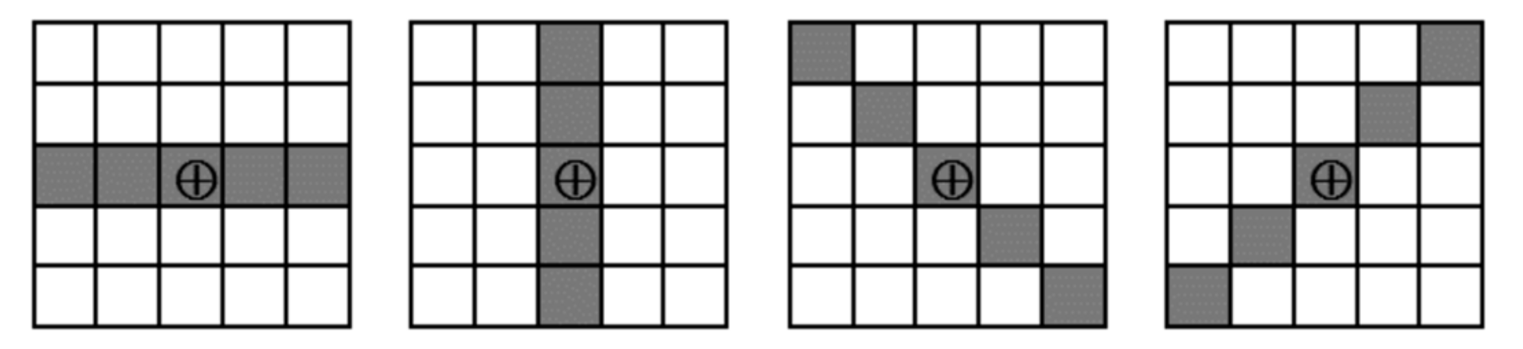
The first filter, applied on the L* component of the image, computes the 2D total variation using four 5 × 5 symmetrical neighborhoods oriented in the four directions, as shown in Figure 6. One calculates the 1D total variation by applying Equation (1) along each line, and then one keeps the maximum of the four values. Then, in order to emphasize the hemangioma area (which is darker than the rest of the skin), we add (maxL − L(i,j)) to the TV value, where maxL is the maximum intensity value from the L* plane, and L(i,j) is the pixel’s luminance. Figure 8c shows an example of such a TV image (for a better visualization, the image is negativized), obtained by applying the filter on the image from Figure 8b.

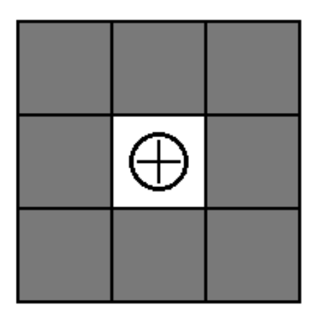
The second filter, also applied on the L* component of the image, computes the 2D total variation by sweeping Equation (1) along the edges of a 3 × 3 symmetrical neighborhood. Here also, in order to emphasize the hemangioma, we add (maxL − L(i,j)) to the TV value. In Figure 8d, one can see the (negativized) result of applying this filter on the image on Figure 8b.

We implemented the following segmentation algorithm:

• construct a seven-plane image composed of:

  -

  the L* component of the image;

  -

  the a* plane;

  -

  the b* plane;

  -

  the TV image obtained by applying the first filter on the L* component of the image;

  -

  the TV image obtained by applying the second filter on the L* component of the image;

  -

  the H plane from HSV (shifted with 50° in order that the red color is not on the transition from 0° to 360°); and

  -

  the S plane from HSV;

• create a binary mask A, which keeps only the reddish pixels (that have the red component from RGB bigger than the green and blue components; an example of a pixel belonging to a hemangioma: R = 152, G = 61, B = 35), that can be hemangioma pixels, by setting a threshold of 85% from the maximum value of the a* plane from (L*a*b*); note that in L*a*b* there is a symmetrical distribution of colors in the a*b* planes;
• multiply each TV image with the mask A to keep only the hemangioma pixels and possibly also some reddish healthy skin pixels;
• apply the Karhunen-Loeve transform on the seven-plane image, and keep only the first five most important planes;
• run the K-means clustering on the five-plane image obtained in the previous step, with a number of 6 classes (the best number of classes was experimentally determined);
• from the segmented image, choose as the hemangioma class the one that has the maximum a* average value, or if there are two regions with the same a* average, choose the one that has the maximum TV (computed with the first filter) value;
• eliminate the obtained hemangioma regions that are smaller than a threshold, or the ones with weak borders.

The last step of the algorithm is necessary because there may be a confusion between hemangioma regions and under-illuminated skin regions that have almost the same color and are a bit textured. To discriminate between these skin regions and the hemangioma region, we implemented a measure of border strength (to extract the objects border, we subtract the eroded objects from their dilated version; we use symmetrical disk-shape structuring elements). Thus, the hemangioma region has strong borders, and we can eliminate the skin regions by keeping only the areas that have the median of the gradient on the edges (we used the Sobel operator) above a certain threshold. The threshold value was determined experimentally.

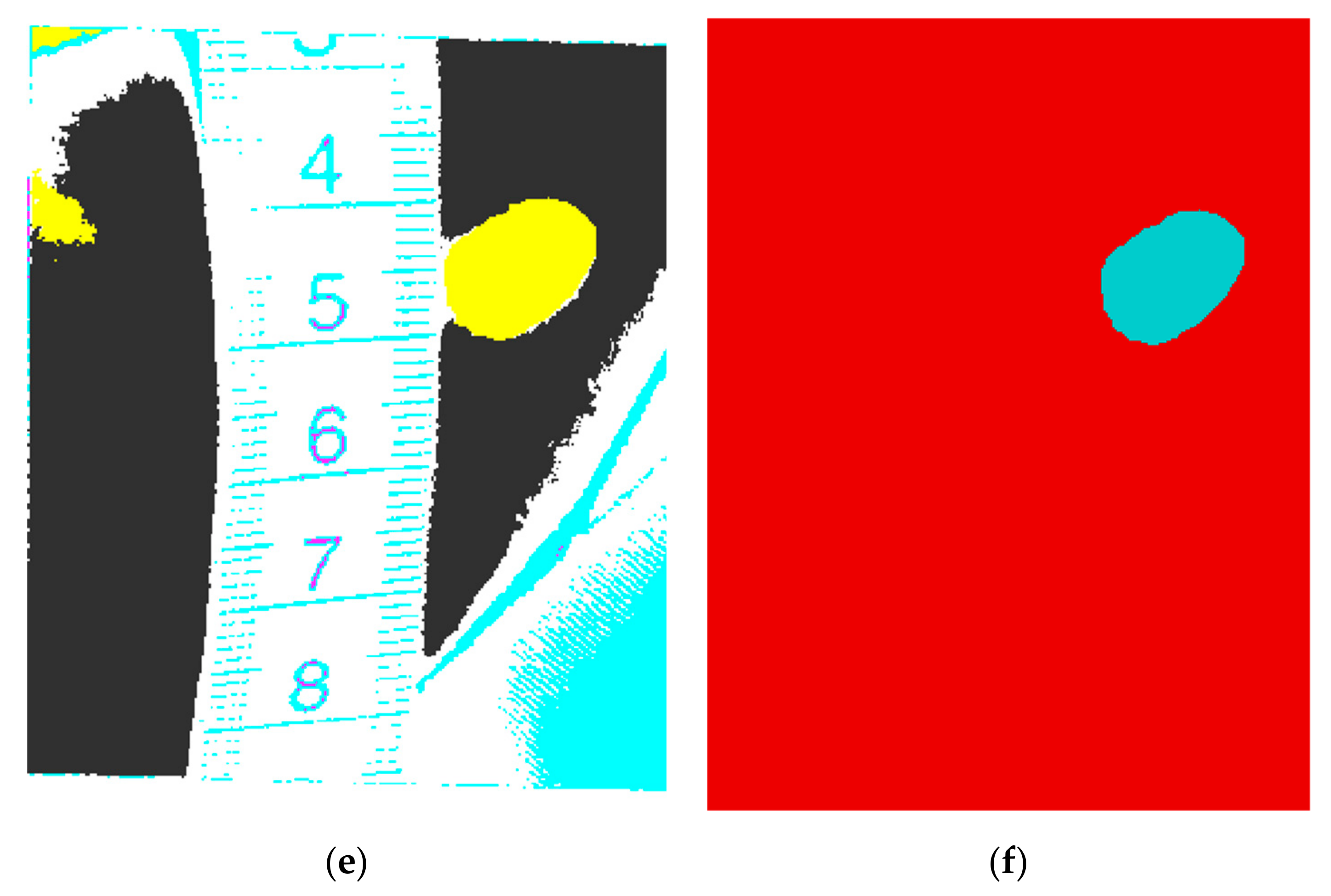
Figure 8a presents the rotation of the original image, rotation performed such that the ruler becomes vertical. In this example the digit five was identified by the OCR and used for the geometric correction, because it is the closest digit to the lesion. In Figure 8b the image obtained after the geometric transformation is shown.

The result of the K-means segmentation with 6 classes is presented in Figure 8e, and the final segmentation result is shown in Figure 8f.

After the segmentation, one can compute the area of the hemangioma by using the formula: area = nb_pixels * pixel_area = nb_pixels/(d * d). For instance, for the lesion presented in Figure 8, the hemangioma surface was calculated as 0.8 cm², which is accurate. It is important to calculate the region’s area accurately, because one can compare this area on further examinations, and decide if there is a progression or a regression of the hemangioma.

The pseudocode of the proposed hemangioma segmentation method is presented in Algorithm 1. The names of the variables from this pseudocode are not the names of the variables within the original Matlab program.

Algorithm 1 The proposed method for hemangioma segmentation

Read the color input image I G ← graylevel(I) BW ← Canny_edge_detection(G) Apply the Hough transform for lines on BW Compute the total variation for each line with Equation (1) Keep the line with the maximum TV value d ← median distance between two consecutive peaks on the line Rotate(I), such as the extracted line becomes vertical M ← extracted digits from the ruler using K-means clustering with 2 classes M ← eliminate objects from M that are too small or too big to represent digits D ← edge density image, obtained by convolving BW with a blurring kernel B ← binary image, where value 1 = if pixel is 45% of the highest contour density from D B ← pixels from B that have R (from RGB) 55% higher than G and 55% higher than B [Bx, By] ← mean location of the pixels with value 1 from B (lesion location estimation) Apply OCR on each region from M; choose the digit from 2 to 9 that is the closest to [Bx, By] Find the key points on the digit I ← geometrical transformation of I, using Equation (2) A1 ← L* from L*a*b* version of I A2 ← a* from L*a*b* version of I A3 ← b* from L*a*b* version of I A4 ← image obtained by applying the first TV filter on L* A5 ← image obtained by applying the second TV filter on L* A6 ← H from HSV (shifted with 50°) A7 ← S from HSV N ← 85% * max(a*), a binary mask where 1 = reddish pixels, 0 = other pixels A4 ← A4 pixelwise multiplied by N A5 ← A5 pixelwise multiplied by N A ← [A1 A2 A3 A4 A5 A6 A7] (7 plane image) X ← Karhunen-Loeve(A), keep only the 5 most important planes Y ← K-means(X), 6 classes S ← binary image, where 1= hemangioma class from Y S ← S without regions smaller than a threshold S ← only regions from S with strong borders R ← compute the lesion surface (number of pixels of value 1 from S * 1/d2)

3. Results

The automatic image scale computation described above was tested for all the images in the database, and worked without errors (the distance between two consecutive gradations on the ruler was correctly estimated for all the images). The estimation of the ruler direction was within a three degrees angle for all the images, which proves that the method is robust. The correct measurement line was identified for all the images, even in the presence of objects having the same color as the ruler in the image. We inspected the geometrically-transformed digit to its ideal frontal template, and there was a precise match, which proves that the geometric correction worked for all the images.

For all the images in the database, we had a manual segmentation (“ground truth”) image, which represents a binary image where the hemangioma pixels are white and the other pixels are black. The accuracy of the segmentation algorithm was assessed in terms of border error (BE), as in [6]. The BE was calculated using the following formula:

BE = Area((A ∪ M) − Area(A ∩ M))/Area(M)

(3)

where A is the hemangioma region obtained after the segmentation, and M is the manual segmented region (from the ground truth).

Here, the term “border” in BE does not mean that the segmentation errors are measured only at the border of the lesions, but, as one can see in formula (3), any surface difference between A and M will increase BE (for instance if the lesion in A has some holes that are not present in M); hence, the term BE was only used with respect to [6].

In practice, it is almost impossible for BE to become 0%, because there are several geometrical uncertainties [18]. For instance, there is some uncertainty when constructing M and there is an uncertainty of the lesion border given by the image acquisition system.

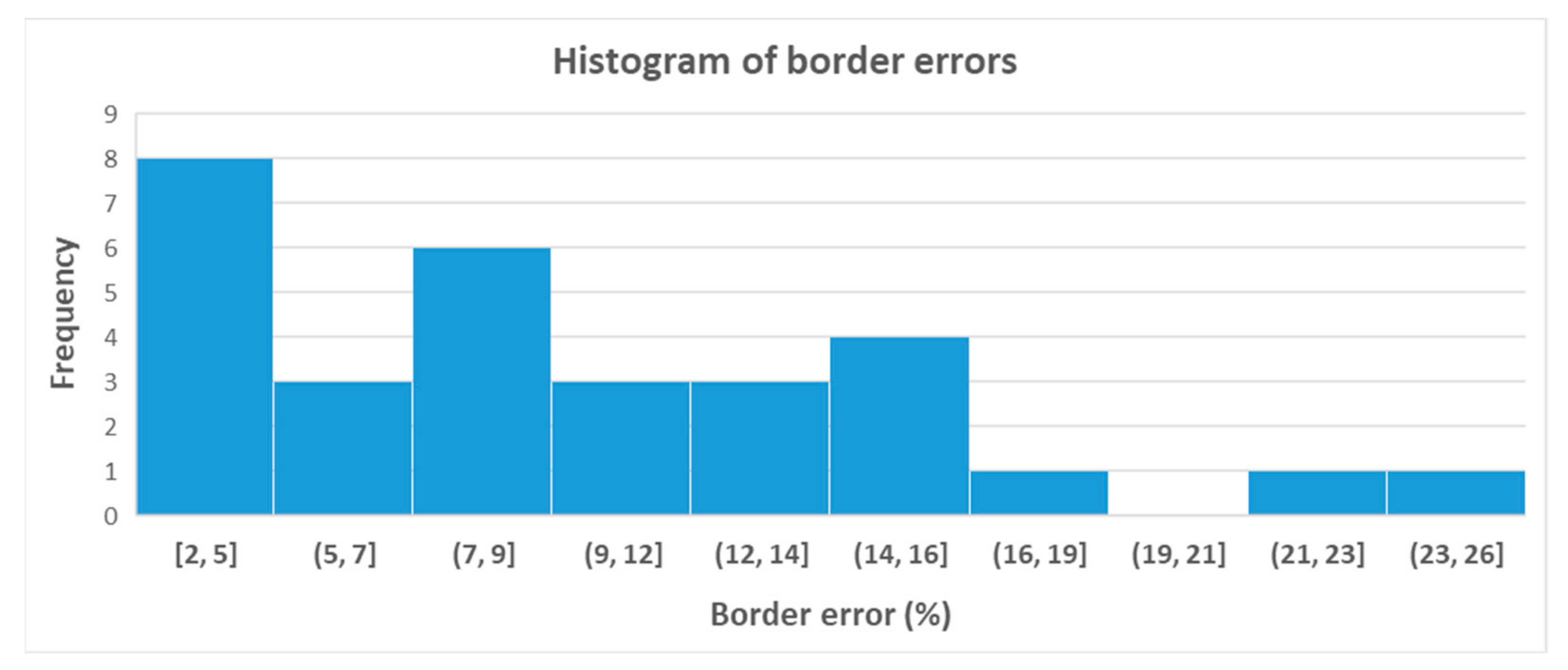
The mean BE for all the images in the database was 9.31%. The minimum BE value was 2.16% and the maximum BE value was 25.64%. This high BE value was obtained on an image where the hemangioma is very small and fragmented, some portions being very similar to the skin; in this case, the morphological opening filter that we used to remove noise also removed some small fragments of the segmented hemangioma.

Figure 9 shows the histogram of border errors for all the images. One notices that for 93% of the images, the BE is smaller than 20%.

As a comparison, the mean BE obtained in [14], without the mean-shift filtering, was 14.6%. Hence, the presented improved algorithm has a better accuracy.

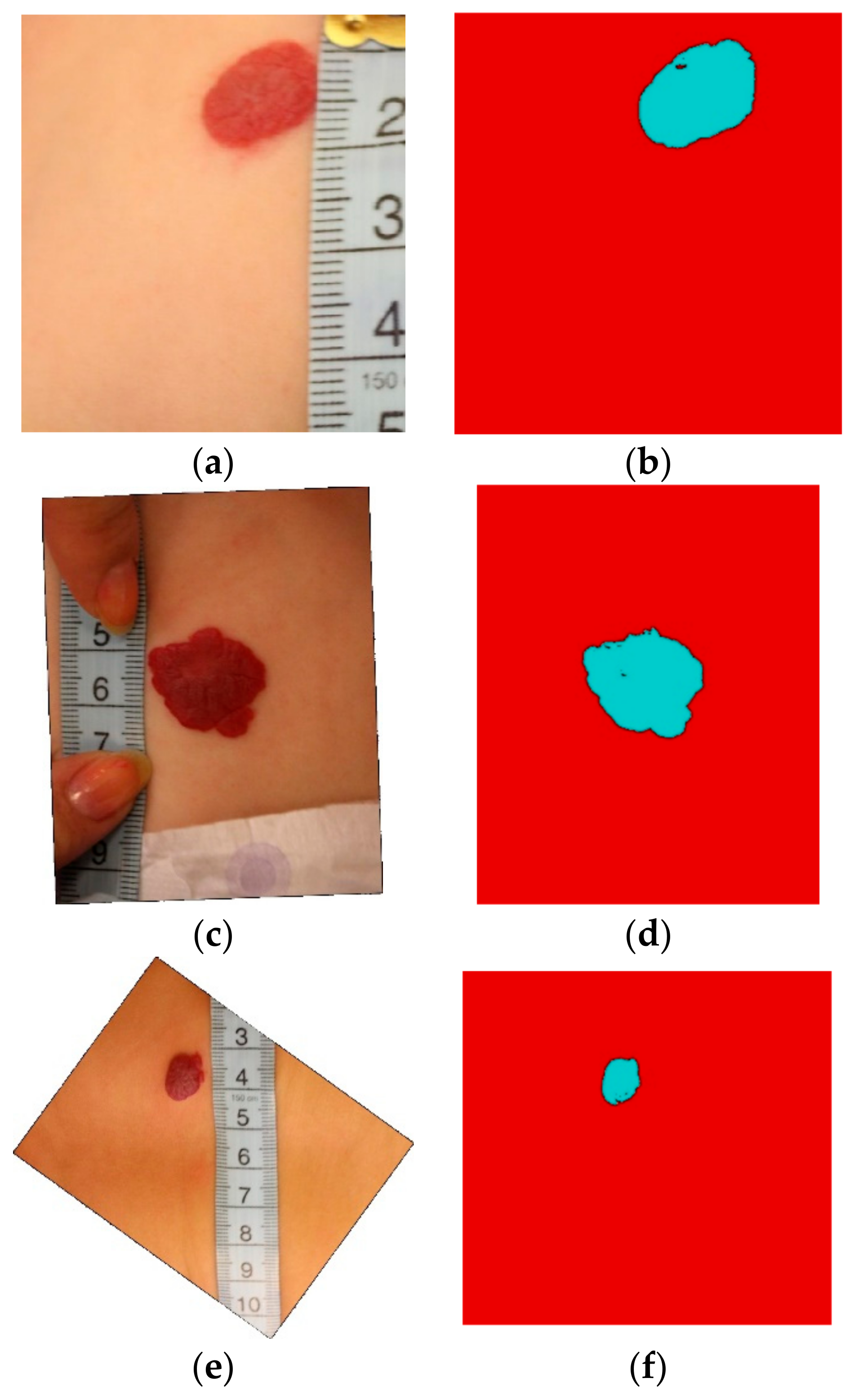
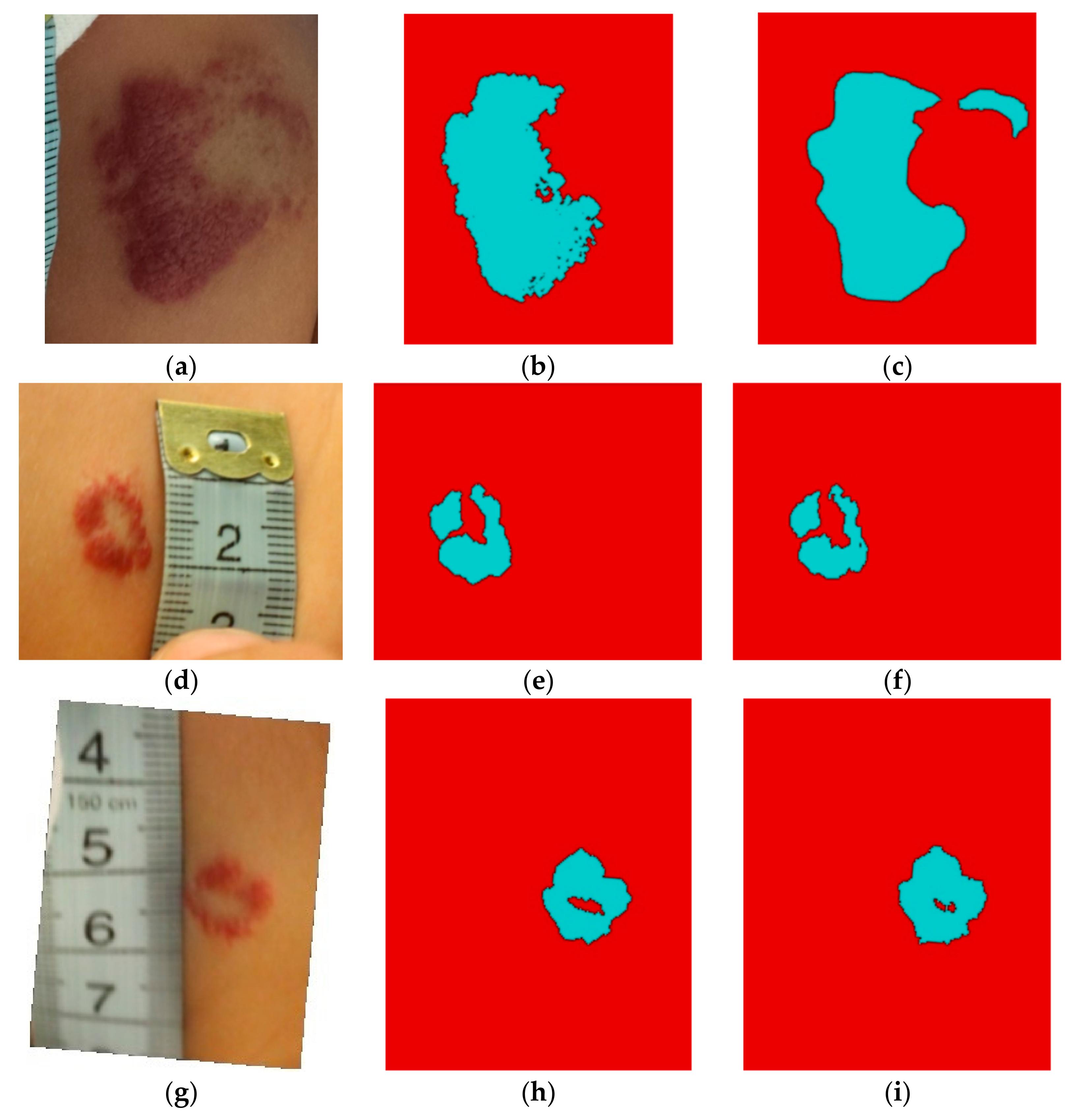
Figure 10 presents three of the best segmentations. These are well defined lesions, and there is a strong color and brightness contrast between the hemangioma and the skin. In Figure 11 three of the worst segmentations are shown. In these images, the contrast between the lesion and the skin is very low.

Comparison of the Obtained Results with Other Methods

We compared the segmentation accuracy (in terms of border error) with four other segmentation methods, as depicted in

Table 1. Border error and computational time values obtained on the same image database with other segmentation methods.

	MAP-Markov [9]	RG-FCM [10]	SOM-MMRNC [11]	Method from [14]	Proposed Method
BE	20.3%	15.5%	14.8%	14.6%	9.31%
Comp. time	40.82 s	13.08 s	420 s	10.2 s	8.36 s

.

The MAP-Markov segmentation method from [9] applied on the current dataset gives the worst results, perhaps because this method is a supervised segmentation that relies on the automatic selection of the training set. The algorithm presented in [9] includes an automatic learning step for the two classes: hemangioma and non-hemangioma; the pixels belonging to regions with maximum edge density and having red color predominance are chosen for learning the hemangioma class. The result of the MAP segmentation is improved by regularization with discrete Markov fields.

The RG-FCM proposed in [10] is an improved region growing algorithm based on FCM, and gives better results than that of FCM. The seeds used as starting points in region growing are computed from the means obtained by applying FCM combined with a threshold based on the minimum value of the hemangioma class and the maximum value of the non-hemangioma class. As stated by the authors of [11], the SOM-MMRNC (self-organizing map followed by a morphological method of reducing the number of classes) method performs better than does FCM, and this can be seen also in Table 1. The SOM neural network is capable of discovering by itself features and patterns of the input data. In [11], a 5 × 5 neurons network was used, the input data being the a* plane from CIE-L*a*b*. The 25 neurons were ordered by the most hemangioma-like prototype obtained, then 25 masks were constructed with a cumulative effect of the ordered neurons Ni (mask i = N1 and N2,…, and Ni). The smoothest mask was chosen as the segmentation result, the smoothness being computed by morphological closing and opening. As another comparison, even though the databases are different, in [6] a mean BE of 32.1%, with a minimum value of 3.6% and a maximum value of 247.7% were reported.

In terms of computing performance, for an image of 1255 × 1325 pixels, on an average i7 (4600u @2.1GHz) processor laptop, the runtime of the segmentation program was around 9 s, as one can see in Table 1, where the computation time (in seconds) is given as a comparison with the other four methods, for the same image.

4. Discussion

In this paper we presented a method for the automatic computation of the IH lesion surface, having as input digital photographs that also contain a ruler near the lesion. The size of a mm in pixels was computed with the use of the Hough transform for lines and the total variation, to select the line that has the maximum mm gradations.

As pre-processing, a geometric correction was introduced to ensure that the lesion is viewed as perpendicular to the camera. This step is necessary for an accurate assessment of the lesion’s size and shape, for further estimation of the hemangioma evolution in time. The geometric correction is performed automatically, by applying a transformation between some key points from a digit (on the ruler) near the lesion, and the corresponding key points on an ideal digit template.

The image segmentation relies on K-means clustering, which receives as input a five-plane image obtained by selecting the five most significative planes from seven image planes with the use of the Karhunen-Loeve transform. Two of the seven image planes characterize the texture, with the help of two specially designed 2D total variation filters: a 5 × 5 neighborhood filter and a 3 × 3 one. In order to eliminate from the segmentation result skin regions that have the same color and texture as the hemangioma, a border detector was implemented, which keeps only the hemangioma regions (that have strong borders).

Our method was compared with four other segmentation methods, on the same dataset, and we obtained the best results.

A limitation of the current method are the relatively poor image-acquisition conditions. The images from the database were acquired over a long period of time (around two years) because the number of IH cases is limited; also, small children do not stand still for photographs, which makes the acquisition process harder.

In terms of accuracy, the proposed algorithm offers better results than the one presented in [14], with a decrease in border error of around 5%.

References

- Shwayder, T.; Schneider, S.L.; Icecreamwala, D.; Jahnke, M.N. Infantile Hemangiomas. In Longitudinal Observation of Pediatric Dermatology Patients; Springer: Cham, Switzerland, 2019. [Google Scholar] [CrossRef]
- Group, T.H.I.; Haggstrom, A.N.; Drolet, B.A.; Baselga, E.; Chamlin, S.L.; Garzon, M.C.; Horii, K.A.; Lucky, A.W.; Mancini, A.J.; Metry, D.W.; et al. Prospective Study of Infantile Hemangiomas: Demographic, Prenatal, and Perinatal Characteristics. J. Pediatrics 2007, 150, 291–294. [Google Scholar] [CrossRef]
- Chang, L.C.; Haggstrom, A.N.; Drolet, B.A.; Baselga, E.; Chamlin, S.L.; Garzon, M.C.; Horii, K.A.; Lucky, A.W.; Mancini, A.J.; Metry, D.W.; et al. Growth Characteristics of Infantile Hemangiomas: Implications for Management. Pediatrics 2008, 122, 360–367. [Google Scholar] [CrossRef] [PubMed] [Green Version]
- Rogowska, J. Chap. 5—Overview and Fundamentals of Medical Image Segmentation. In Handbook of Medical Image Processing and Analysis, 2nd ed.; Bankman, I.N., Ed.; Academic Press: Cambridge, MA, USA, 2009; pp. 73–90. [Google Scholar] [CrossRef]
- Gillmann, C.; Post, T.; Wischgoll, T.; Hagen, H.; Maciejewski, R. Hierarchical image semantics using probabilistic path propagations for biomedical research. IEEE Comput. Graph. Appl. 2019, 39, 86–101. [Google Scholar] [CrossRef] [PubMed]
- Zambanini, S.; Sablatnig, R.; Maier, H.; Langs, G. Automatic image-based assessment of lesion development during hemangioma follow-up examinations. Artif. Intell. Med. 2010, 50, 83–94. [Google Scholar] [CrossRef] [PubMed]
- Sultana, A.; Zamfir, M.; Ciuc, M.; Oprisescu, S.; Popescu, M. Automatic segmentation of infantile hemangiomas. In Proceedings of the Signals, Circuits and Systems (ISSCS), International Symposium on, Iasi, Romania, 9–10 July 2015; IEEE: New York, NY, USA, 2015; pp. 1–4. [Google Scholar] [CrossRef]
- Sultana, A.; Oprisescu, S.; Ciuc, M. Automatic evaluation of hemangiomas for follow-up monitoring. In Proceedings of the E-Health and Bioengineering Conference (EHB), Iasi, Romania, 19–21 November 2015; IEEE: New York, NY, USA, 2015; pp. 1–4. [Google Scholar] [CrossRef]
- Oprisescu, S.; Ciuc, M.; Sultana, A.; Vasile, I. Automatic segmentation of infantile hemangiomas within an optimally chosen color space. In Proceedings of the E-Health and Bioengineering Conference, Iasi, Romania, 19–21 November 2015; IEEE: New York, NY, USA, 2015; pp. 1–4. [Google Scholar] [CrossRef]
- Neghina, C.; Zamfir, M.; Sultana, A.; Ovreiu, E.; Ciuc, M. Automatic detection of hemangiomas using unsupervised segmentation of regions of interest. In Proceedings of the Communications (COMM), 2016 International Conference on, Bucharest, Romania, 9–10 June 2016; IEEE: New York, NY, USA, 2016; pp. 69–72. [Google Scholar] [CrossRef]
- Neghina, C.; Zamfir, M.; Ciuc, M.; Sultana, A. Automatic detection of hemangioma through a cascade of self-organizing map clustering and morphological operators. Procedia Comput. Sci. 2016, 90, 145–150. [Google Scholar] [CrossRef] [Green Version]
- Alves, P.G.; Cardoso, J.S.; Bom-Sucesso, M.D. The Challenges of Applying Deep Learning for Hemangioma Lesion Segmentation. In Proceedings of the 2018 7th European Workshop on Visual Information Processing (EUVIP), Tampere, Finland, 26–28 November 2018; pp. 1–6. [Google Scholar] [CrossRef]
- Sultana, A.; Balazs, H.; Ovreiu, S.; Oprisescu, S.; Neghina, C. Infantile Hemangioma Detection using Deep Learning. In Proceedings of the 2020 13th International Conference on Communications (COMM), Bucharest, Romania, 18–20 June 2020; pp. 313–316. [Google Scholar] [CrossRef]
- Oprisescu, S.; Ciuc, M.; Sultana, A. Automatic measurement of infantile hemangiomas. In Proceedings of the 2017 E-Health and Bioengineering Conference (EHB), Sinaia, Romania, 22–24 June 2017; pp. 503–506. [Google Scholar] [CrossRef]
- Smith, R. An Overview of the Tesseract OCR Engine. In Proceedings of the Ninth International Conference on Document Analysis and Recognition (ICDAR 2007), Parana, Brazil, 23–26 September 2007; Volume 2, pp. 629–633. [Google Scholar]
- Sosa, N.L.D.; Noguera, J.L.V.; Silva, J.J.C.; Torres, M.G.; Ayala, H.L. RGB Inter-Channel Measures for Morphological Color Texture Characterization. Symmetry 2019, 11, 1190. [Google Scholar] [CrossRef] [Green Version]
- Ndajah, P.; Kikuchi, H. Total variation image edge detection. In Proceedings of the 10th WSEAS International Conference on Electronics, Hardware, Wireless and Optical Communications; Springer: New York, NY, USA, 2011; pp. 246–251. [Google Scholar]
- Gillmann, C.; Wischgoll, T.; Hamann, B.; Ahrens, J. Modeling and Visualization of Uncertainty-Aware Geometry Using Multi-variate Normal Distributions. In Proceedings of the 2018 IEEE Pacific Visualization Symposium (PacificVis), Kobe, Japan, 10–13 April 2018; pp. 106–110. [Google Scholar] [CrossRef]
Figure 1.
Example of images from the database.
Figure 2.
(a) All the detected lines and the selected line (in blue); (b) The intensity profile (reversed) along the selected line.
Figure 3.
The eight digits used as reference for the geometric transformation and the key points defined on them.
Figure 4.
The processing steps for digit five: (a) original image; (b) binarization; (c) skeletonization and setting of the key points.
Figure 5.
The estimation of the curvature for the digit five. The peaks correspond to key points 3 and 1 from Figure 4.
Figure 6.
The four 5 × 5 oriented neighborhoods used to compute the total variation for the first filter.
Figure 7.
The 3 × 3 neighborhood used to compute the total variation for the second filter.
Figure 8.
(a) The rotation of the original image; (b) the geometrically-transformed image; (c) the total variation (TV) image with the first filter (shown in negative); (d) the TV image with the second filter; (e) K-means segmentation with 6 classes; (f) final segmentation result.
Figure 9.
The histogram of border errors.
Figure 10.
(a) Original image #1; (b) Segmented version of #1, border error (BE) 2.16%; (c) Original image #2; (d) Segmented version of #2, BE 2.75%; (e) Original image #3; (f) Segmented version of #3, BE 3.14%.
Figure 11.
(a) Original image #1; (b) Segmented version of #1, BE 25.64%; (c) Ground truth for #1; (d) Original image #2; (e) Segmented version of #2, BE 21.75%; (f) Ground truth for #2; (g) Original image #3; (h) Segmented version of #3, BE 16.44%; (i) Ground truth for #3.