
On the Application of a Design of Experiments along with an ANFIS and a Desirability Function to Model Response Variables

Materials and Manufacturing Engineering Research Group, Engineering Department, Public University of Navarre, Campus de Arrosadía s/n, 31006 Pamplona, Navarra, Spain
Symmetry 2021, 13(5), 897; https://0-doi-org.brum.beds.ac.uk/10.3390/sym13050897
Submission received: 22 April 2021
/
Revised: 13 May 2021
/
Accepted: 14 May 2021
/
Published: 18 May 2021
(This article belongs to the Special Issue Symmetry in Manufacturing Systems Engineering — Concept and Theory to Improve Design, Process, Quality and Circularity as the Basis for Future Manufacturing Philosophy)
Abstract
:In manufacturing engineering, it is common to use both symmetrical and asymmetrical factorial designs along with regression techniques to model technological response variables, since the in-advance prediction of their behavior is of great importance to determine the levels of variation that lead to optimal response values to be obtained. For this purpose, regression techniques based on the response surface method combined with a desirability function for multi-objective optimization are commonly employed, since it is usual to find manufacturing processes that require simultaneous optimization of several variables, which exhibit in many cases an opposite behavior. However, these regression models are sometimes not accurate enough to predict the behavior of these response variables, especially when they have significant non-linearities. To deal with this drawback, soft computing techniques are very effective in overcoming the limitations of conventional regression models. This present study is focused on the employment of a symmetrical design of experiments along with a new desirability function, which is proposed in this study, and with soft computing techniques based on fuzzy logic. It will be shown that more accurate results than those obtained from regression techniques are obtained. Moreover, this new desirability function is analyzed in this study.
1. Introduction
In manufacturing engineering, it is necessary to model the behavior of response variables as a function of several input variables in order to be able to select the most suitable operating conditions in advance. However, this selection of optimal operating conditions sometimes conflicts with the desired levels of variation for the response variables, since the levels of the independent variables that can optimize a given output (for example, the surface roughness or the wear of a tool) can conflict with those that optimize another different one (for example, the material removal rate). Therefore, the optimal selection of operating conditions is not an easy task and it is necessary to use statistical tools for modeling of the response variables versus variations in the process parameters. This can sometimes lead to a high number of experiments being carried out, and therefore it is common practice to employ design of experiments techniques that allow, with a relatively small number of experiments, some very useful information on the behavior of the variables under study to be obtained. In this way, response surface method (RSM), artificial neuronal networks (ANN), fuzzy inference systems (FIS) [1,2], and adaptive neural fuzzy inference system (ANFIS) [3] have been widely employed. With regard to fuzzy inference systems, Takagi-Sugeno [1] and Mamdani [2] are the most commonly employed. Several studies can be found in the literature dealing with the application of these aforementioned techniques [4,5,6].
Fuzzy inference systems (FIS) have been employed in several scientific fields, for example, dealing with modeling of material removal in abrasive belt grinding processes, as shown in Pandiyan et al. [7], classification of defects, as shown in Versaci [8] and in Burrascano et al. [9], to improve talc pellet manufacturing processes [10] and to predict the compressive strength of cement [11]. Further examples can be found in [12,13,14], among many others. In order to use the above-mentioned models, it is quite common to employ symmetric designs, in which all the factors have the same levels of variation as well as asymmetric ones, where not all the factors have the same levels of variation [15,16]. In manufacturing engineering 2k, 3k, and 4k symmetric designs are commonly used, because a large amount of information is available from a relatively small number of experiments. As a consequence of the technological interest of modeling output variables in manufacturing processes, a large number of models have been developed in recent years based both on conventional regression techniques and on the use of soft computing, both through fuzzy inference systems and through neural networks, generally by using supervised learning and feed forward networks. It should be underlined that when regression models have high values in the coefficients of determination, they may approach the behavior of response variables with relatively high accuracy. However, when the response variables exhibit high non-linearities, conventional regression models are not capable of modeling the behavior of output variables adequately and hence some other types of techniques need to be employed.
Since it was first proposed by Harrington [17], and later modified by the classification function of Derringer and Suich [18], the methodology of multiple optimization based on the use of a desirability function, has been used in a large number of research studies for the simultaneous optimization of response variables. In this present study a symmetrical 43 factorial design of experiments combined with an ANFIS and a new desirability function is employed. The proposed function to transform the output responses is of an arctangent type, which is analyzed in this present study. The ANFIS along with this new desirability function will be used to determine the values that can approach the optimum value of the independent variables that simultaneously optimize the response outputs.
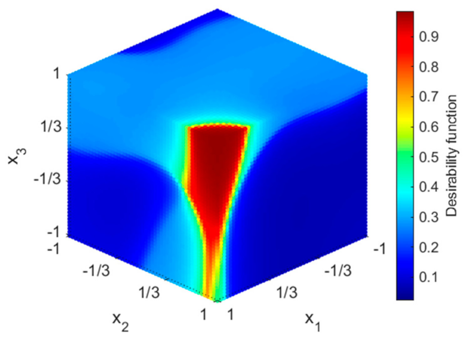
As can be observed in Figure 1, three independent variables x1, x2, and x3 are varied in order to show the values that optimize a desirability function by using a symmetric design of experiments and an ANFIS, following the methodology shown in this present study.
However, as previously mentioned if regression models are not capable of adequately predicting the actual behavior of output variables some other techniques should be used. Moreover, results obtained in this present study will be compared with those obtained with the transformation proposed by Derringer and Suich [18], which is commonly employed by several research studies found in the literature, as will be shown in the Section 3.
2. State of the Art
The research study of Harrington [17] showed how to optimize several variables simultaneously by using a desirability function combined with an exponential classification function. Subsequently, Derringer and Suich [18] proposed a transformation for the optimization of multiple variables simultaneously using a desirability function and assuming that the estimated values are a continuous function of the dependent variables and therefore the desirability function, which they obtain from the geometric mean of the transformed variables in the interval [0,1], is a continuous function of the independent variables [18]. As is stated in the research study of Del Castillo et al. [19], the desirability function approach consists in using response surface methods to fit polynomials for each response variable in order to have a single optimization problem. In their study Del Castillo et al. [19] present modified desirability functions that are differentiable everywhere. This is important because it is quite common for the obtained overall desirability functions obtained from RSM to be non-differentiable, especially when there are several responses and design variables [20]. In the study of He and Zhu [20], the authors propose a hybrid approach, which combines the genetic algorithm with the pattern search method, to deal with this point. In Costa el al. [21] a review on different desirability methods is carried out. Some other authors have proposed several transformation functions. For example, an exponential transformation is suggested by Kim and Lin [22]. In another study, Kros and Mastrangello [23] study the relationship between response types when they are mixed (the larger the better, the smaller the better, and nominal the best). On the other hand, Das et al. [24] employ a genetic algorithm-based optimization to determine the tensile properties of a high-strength low-alloy steel, where multi-layer perceptron ANNs are developed for the output responses and then a desirability function based on employing a sigmoidal function is obtained [24] and Zong et al. [25] combine variations due to noise factors and controllable factors. In another study developed by He et al. [26], a robust desirability function approach to simultaneously optimize multiple responses is proposed. Some other studies are those of Ribardo and Allen [27] that propose a method, which is expressed as a function of the mean and standard deviation of the associated criteria or quality characteristics; that of Wu and Chyu [28] which present an approach to optimizing correlated multiple quality characteristics with asymmetric loss function, that of Ortiz et al. [29] which proposes a multiple-response solution technique using a genetic algorithm in conjunction with an unconstrained desirability function and that of Pasandideh and Niaki [30] which models a multiple variable optimization problem by using the desirability function approach and then they employ four genetic algorithm methods to solve the problem.
On the other hand, Das [31] make use of the property of desirability function in the neural network architecture and evaluate their performances. Three combinations of transfer/desirability functions are analyzed in this study [31]. Lee and Kim [32] proposed a desirability function defined as the average of the conventional desirability values based on the probability distribution of the predicted response variable and in He et al. [33] a robust methodology for response surface analysis, when there are several responses, is studied. Moreover, in their study the authors propose a measure of robustness for second order response surface models [33]. In Lee et al. [34], a desirability function method to simultaneously optimize both the mean and variability of multiple responses is proposed.
Although the desirability function is a very interesting method to simultaneously optimize several variables, the transformation into the desirability space should take the preferences of the decision maker into account in order to obtain the optimal parameters as stated by Fuller and Scherer [35].
Derringer and Suich [18] transformation has been widely employed over the last few years. For example, the use of models based on the use of design of experiments along with the response surface methodology using the Derringer and Suich methodology has been employed in several research studies as shown in Vera et al. [36]. In the research study of Padilla et al. [37] the authors carry out an analysis on the optimization of a spark ignition engine. A 33 design of experiments (DOE) is conducted where the independent variables are the revolutions, the load produced by a dynamometer, and an electrolyte concentration and the response variables are torque, hydrocarbon emissions, and power. In another study, Hur et al. [38] present the results of surface response optimization using the desirability function with a central composite design to determine the design variables to control the distribution of flow rate in a cooling system employed in an electric vehicle. On the other hand, Saleem et al. [39] consider the deflection angle, input power, and micromirror temperature rise from the ambient as response variables to be simultaneously optimized by using response surface models and a desirability function. The application of design of experiments, response surface methodology and a desirability function is also discussed by Akçay and Anagün [40] to model and optimize a manufacturing process. The influence of cutting speed, feed rate, and depth of cut on the machinability characteristics of Si optical lenses is analyzed by Jumare et al. [41]. These authors develop predictive models in order to obtain minimum arithmetical mean roughness and tool wear as well as maximum material removal rate using the desirability function approach [41].
Other studies such as that of Chahal et al. [42] show that RSM along with a desirability function is effective in order to optimize surface roughness in end milling; Zhao et al. [43] analyze the effect of welding parameters on the mechanical properties of welding bead and welding heat input using a DOE and a desirability function and Kribes et al. [44] study the effect of machining conditions on the obtained surface roughness in hard turning by using response surface methodology and a desirability function. Some other studies which employ the response surface methodology and a desirability function are Ahmad et al. [45] that optimizes the recycling conditions of aluminum (AA6061) chips, Qazi et al. [46] that analyzes the machinability of AA5005H34, and Osman et al. [47] that studies continuous multi-pass friction stir welding to clad dissimilar materials. Cutting speed, feed rate, and depth of cut are used as design parameters along with RSM and desirability function in Laghari et al. [48] for modeling cutting forces in the machining of a composite material; Pradhan et al. [49] analyze surface roughness in machining of Al/SiCp metal matrix composite; optimization of friction surface deposition of stainless steel over medium carbon steel is shown in Sahoo et al. [50] and in Du et al. [51] a multi-objective optimization is carried out in the dry machining of a 304 stainless steel, among many others.
The number of studies that exist in the literature related to the combined application of soft computing techniques and desirability functions is much lower. Among these studies, it is worth mentioning that of Mostafaei [52] that employs ANFIS models for prediction of biodiesel fuels cetane number using a desirability function, which employs a linear transformation and a comparison of the developed models is performed by statistical criteria. Another study is that of Labidi et al. [53] where ANN, RSM, and desirability function are used to determine optimal machining conditions in the turning of a hardened steel. On the other hand, Sengottuvel et al. [54] study the effects of various electrical discharge machining input parameters as well as the influence of different tool geometry on material removal rate, tool wear rate, and surface roughness. These authors also develop a fuzzy inference system which is validated with experimental results. Another study worth mentioning is that of Singh et al. [55] where the application of Taguchi’s robust design coupled with fuzzy based desirability function approach for optimizing multiple bead geometry parameters of submerged arc weldment is developed. Response surface methodology and the desirability function results were also employed for modeling Ti-6Al-4V milling under different lubrication conditions in the study of Paschoalinoto et al. [56]. These authors also compared the statistical results with those obtained from using supervised artificial neural networks and they found that both artificial neural network and the experimental design predict similar results [56]. Tank et al. [57] use a desirability function for each of the surface roughness parameters analyzed in the turning of glass fiber reinforced with plastic and then employ a fuzzy inference system to determine values of a characteristic index which then are used to find the signal to noise ratio. In the research study of Salmasnia et al. [58] an approach for optimization of correlated multi-response variables is analyzed. In their study an ANFIS is used as a tool for predicting system behavior. On the other hand, the study of Gajera et al. [59] deals with the application of response surface methodology with fuzzy-based desirability function approach in order to optimize multiple process parameters in direct metal laser sintering, among others.
3. Methodology
As shown in the review of the state of the art, statistical tools based on the design of experiments and the response surface method have been widely used to model the behavior of different response variables and it has also been shown that the use of a desirability function based on RSM and the model proposed by Derringer and Suich [18] have been commonly used in order to simultaneously optimize response variables, since it is usual to find manufacturing processes that require simultaneous optimization of several variables, which exhibit, in many cases, an opposite behavior. In manufacturing processes, is it quite common for certain technological variables to have a more regular response behavior and, therefore, they can be adequately modeled by methodologies such as RSM, and, on the other hand, there also exist some other technological variables that cannot be adequately modeled using conventional regression. These regression models are sometimes not accurate enough to predict the behavior of these response variables, especially when they have significant non-linearities.
In order to address these problems, in this present research study, the use of a new desirability function which is based on the inverse tangent (arctangent) is first proposed to classify the output responses of a design of experiments, so that for each of the response functions a transformed function that lies between [0,1] will be obtained from Equation (1).
where and are first adjusted so that the arctangent function lies between 0 and 1. This is easily obtained from simultaneously solving for and the equations which yields to . Therefore, the transformation to be used in this present study is given by Equation (2).
The values of constants and will be selected depending on the desired level for each variable (maximize, minimize, or lying within a range of values).
In the event that the desired variation of an output response ( is its maximum value, the constants of Equation (2) will be given by Equations (3) and (4).
where for the case of a variable whose preferred level is the maximum () is defined from Equation (5), where is a constant which can be used to set at a specific point (default value and is defined to fix the value of the arctangent at this point. Moreover, the value of the constant is selected, for simplicity, to be a multiple of the difference between the maximum and the minimum . Then is set by using the constant , as Equation (6) shows (however, this value could be selected in whatever different way) and it is selected in order to set the transition of the output variable to the level of “1”. As previously mentioned, are the maximum and the minimum levels of each variable. In this present study these values will be selected from the DOE, however they could be whatever.
Analogously, if the preferred level of an output variable is the minimum, the , and constants as well as are obtained from Equations (7)–(10) respectively, so that if the output variable is close to its minimum value (), then the transformed function will approach to “1” and, on the contrary, if the value of this variable approach the maximum, in this case non-desirable value, then the transformed output will correspond to a value close to “0”, where the sub-index “t” in the transformed variable refers to an output variable transformed by using the arctangent function, as previously shown.
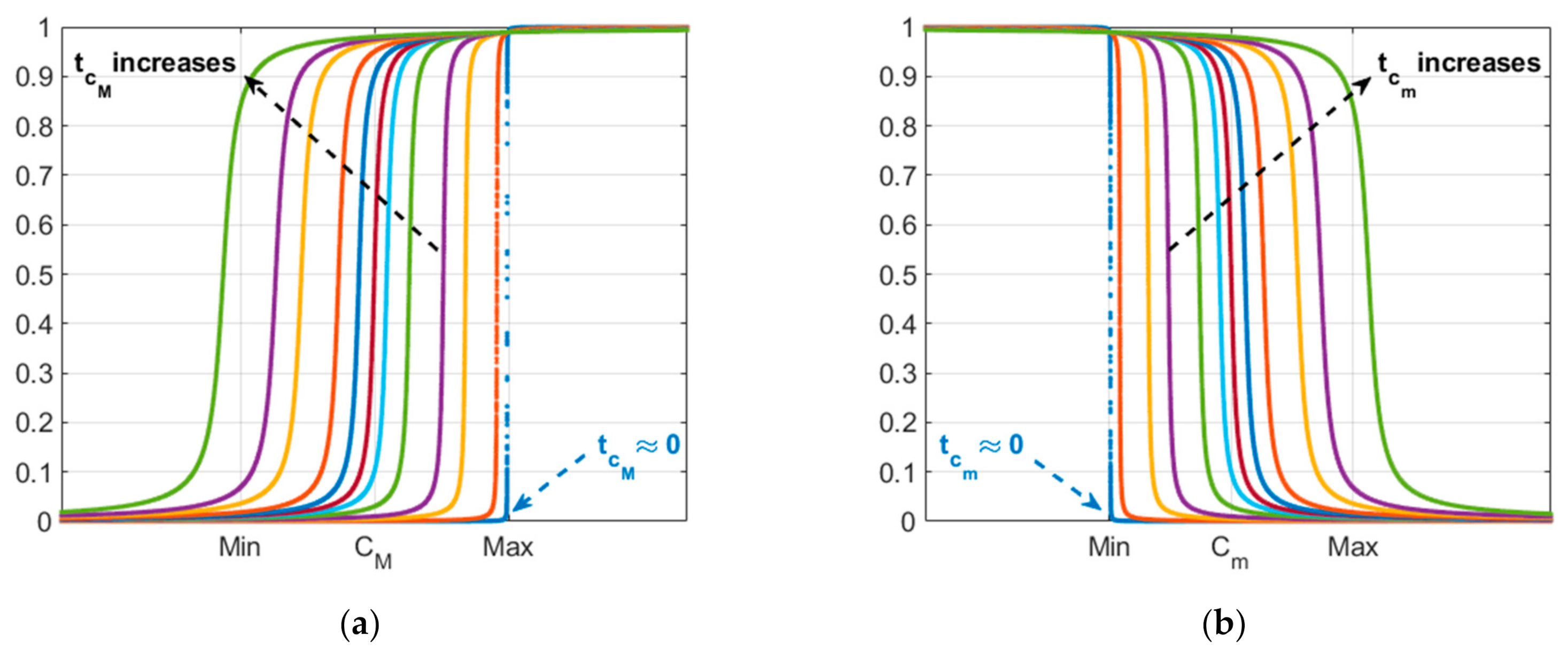
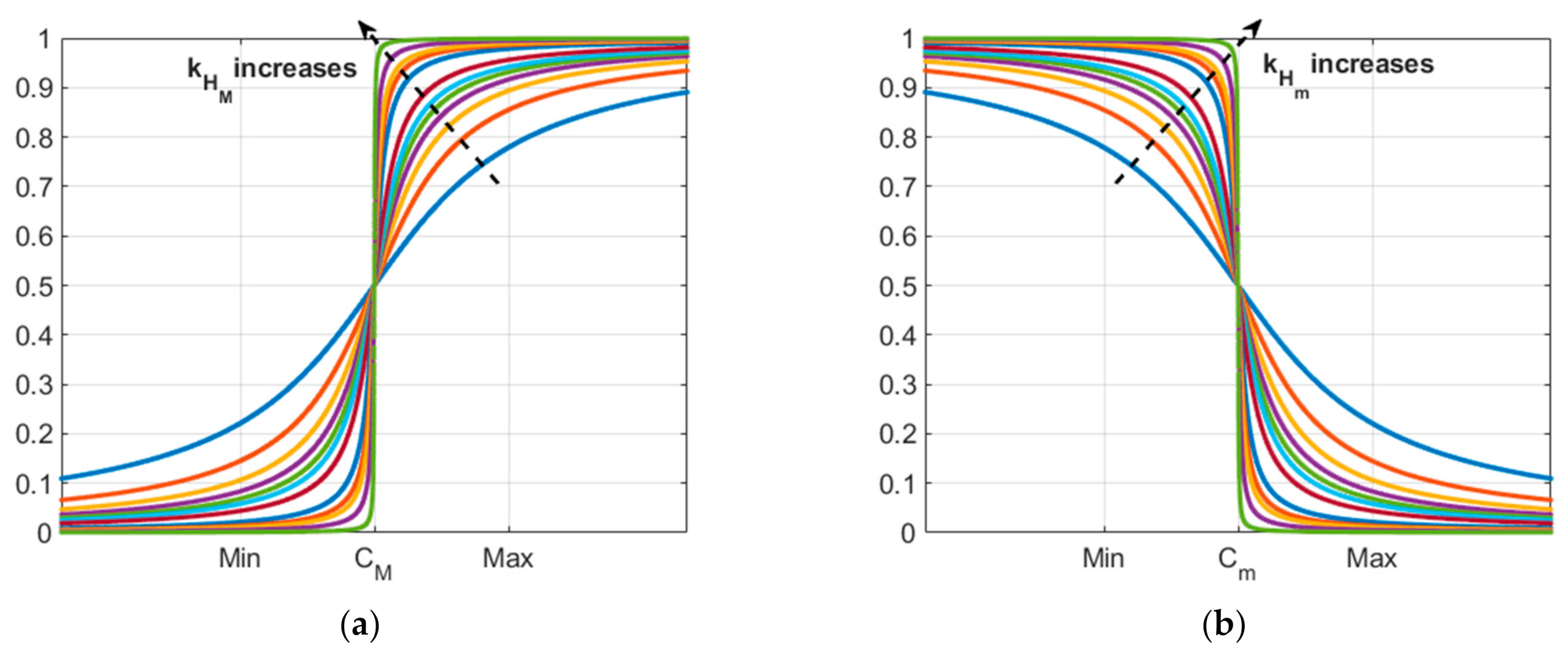
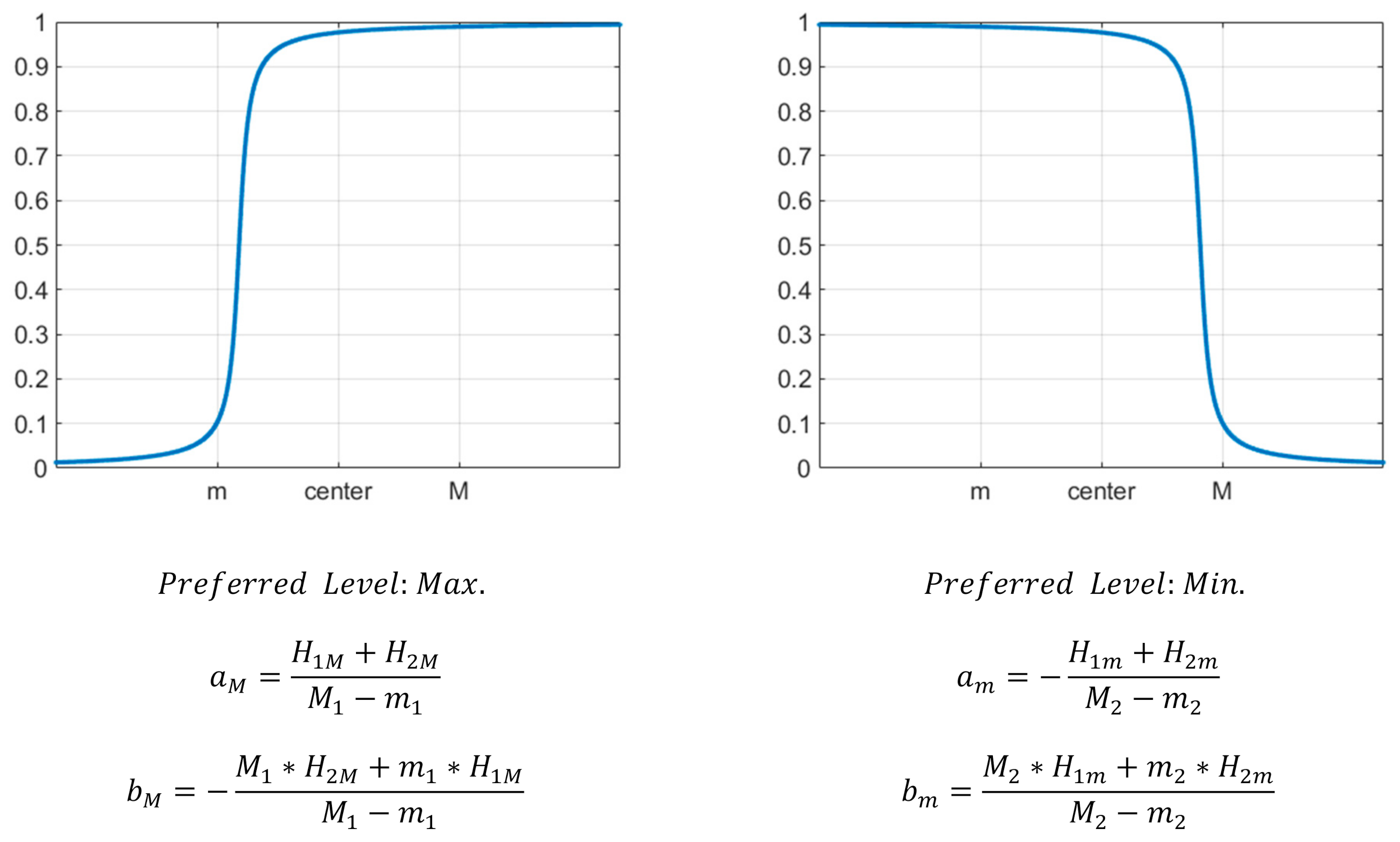
As previously mentioned, (, are defined from Equation (5), when the preferred level of a variable is its maximum, and from Equation (9), when the preferred level is its minimum. Moreover, a weighted average can be used to set ( at a specific point by using constants, respectively. The influence of these constants is shown in Figure 2. The parameter is used to select the transition to the “1” value of the transformed variable. For a given value of , the values of will be selected within the interval given by Equation (11) and by Equation (12), respectively. The influence of and is shown in Figure 3.
are the maximum and the minimum levels of each variable, as previously mentioned. If values of and are selected within the range given by
The shape of the function will be inverted. It could have been possible to select values higher than 1 but it makes no sense for the present parameter because its variation is desired to be within the interval [0, 1]. Finally, the influence of the -parameter is shown in Figure 4. If a given value of the t-parameter (is given, then the value of , which will define the value of or , respectively should be selected within the interval given by Equation (13) and by Equation (14), respectively.
Therefore, the shape of the arctangent transformation can be adjusted by varying (,, (and ( parameters whose influence is respectively shown in Figure 2a, Figure 3a, and Figure 4a, in the case where the preferred level of a response variable is the maximum, and in Figure 2b, Figure 3b, and Figure 4c, in the case where the preferred level of a response variable is the minimum.
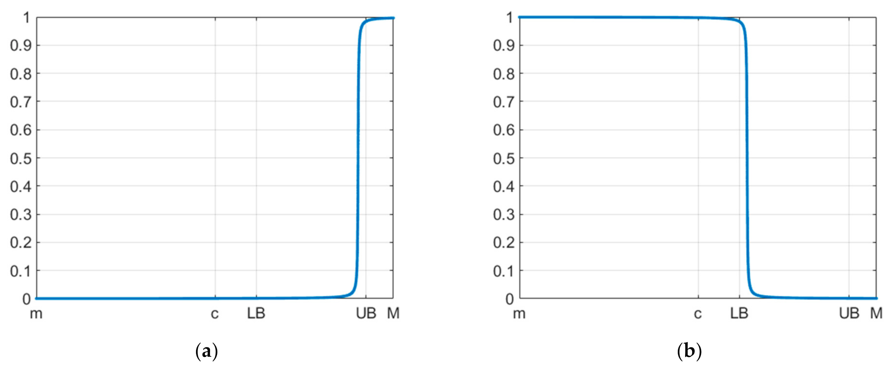
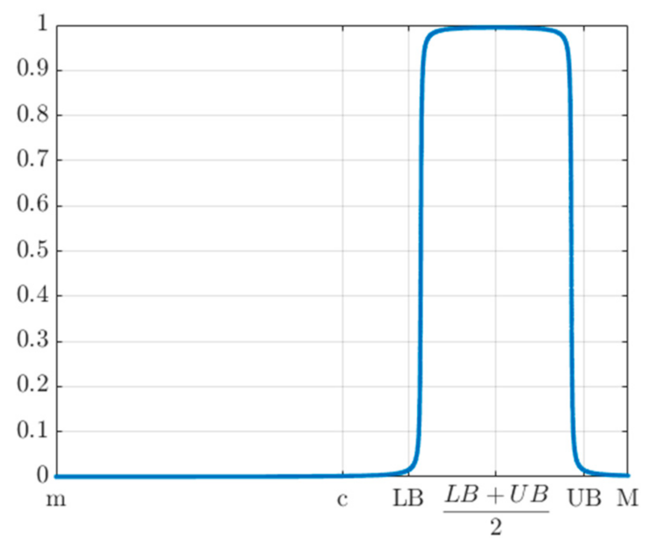
If the output response has to be within a specified range [LB,UB], then it is possible to combine two transformation functions similar to those shown in Figure 5a,b, so that the result attained is shown in Figure 6, where LB and UB are both the lower bound and the upper bound selected.
The shape of the transformed function shown in Figure 6 is obtained from Equation (15), where the midpoint (LB + UB)/2 has been considered. However, this point could be whatever within the specified range [LB,UB]
However, if the output response has to be within the range defined by [LB, UB] and the external values are not acceptable, it is possible to set a value of close to zero, so that results shown Figure 7 will be obtained and then by applying Equation (15) the output shown Figure 8, is obtained.
As can be observed in Figure 8, the variable remains within the specified range. As in the previous case, the shape of the transformed function shown in Figure 8 is obtained from Equation (15).
Note that it could be possible to employ this arctangent function by selecting the levels of the transition to “1” and “0” instead of the method shown below by employing two H-parameter (one to adjust the transition to the “1” level and another to the “0” level). In this case, the obtained values will be those shown in Figure 9. However, parametrization shown in Figure 9 will not be used in this present study and the methodology previously shown will be used instead.
Once the response variables have been transformed, a mean is selected to be maximized. As was previously shown in the state-of-the-art Section, most of the previously published studies employ the geometric mean, shown by Equation (16). This mean was proposed to be employed in the research study of Harrington [17] and later was used by Derringer and Suich [18], among many others. Although other means could be used in this present study such as the harmonic one, in this present study the geometric mean will be used, without weighting the functions.
A symmetric 43 DOE with three output responses, which will be simultaneously optimized has been considered. However, it should be mentioned that this DOE as well as the output responses could be whatever. From the above, in this present study, one of the response variables is preferred to be at its minimum level, another response variable is preferred to be at its maximum and the third output response has to be within a certain range. With the proposed methodology, it is possible to approximate the optimum that simultaneously optimizes the desired levels of variation of these functions within the range of study under consideration. As shown in Section 2, this is usually done through the use of models based on RSM and most of these studies employ the function proposed by Derringer and Suich [18].
In the present study, the levels of variation of the input variables (process parameters) have been varied into the range as Table 1 shows. By using the DOE shown in Table 1, the results shown in Table 2 are obtained for three output responses that have been named , y , respectively (these values have been generated by using three analytical functions). It should be underlined that either an actual study case or any other function could have been used to carry out this study. As can be observed in Table 2, 43 experiments will be available. The values shown in Table 2 have been rounded to two decimal places.
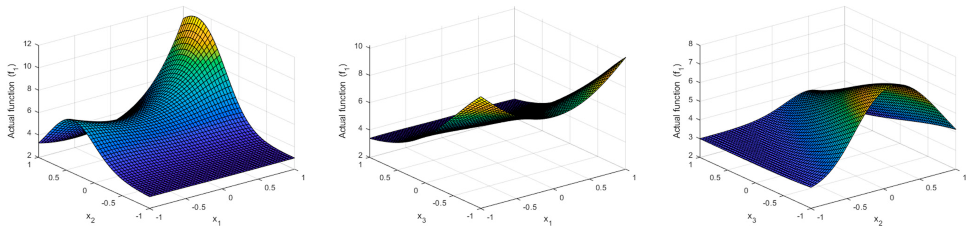
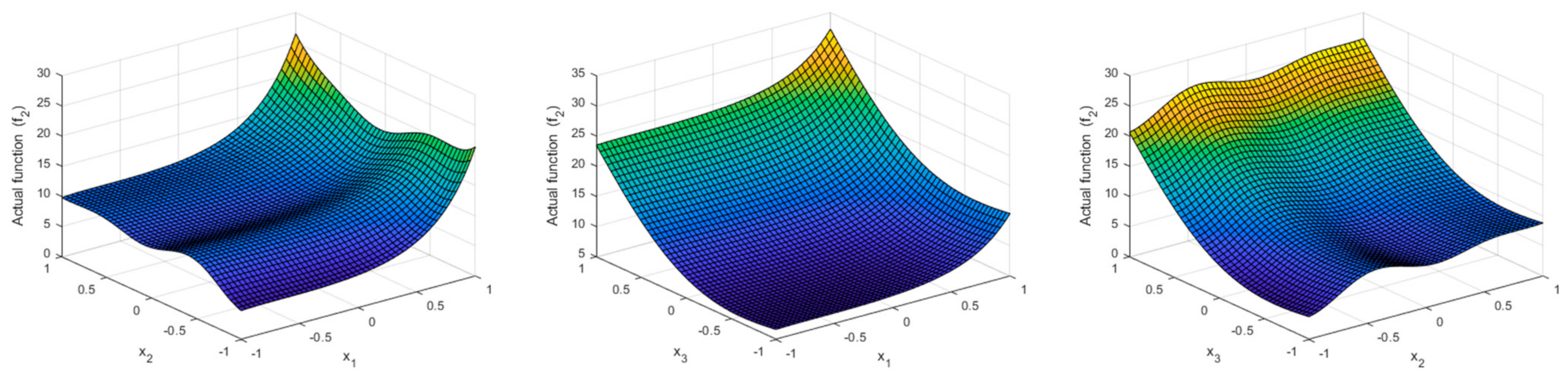
Therefore, from the above, the proposed methodology shown in Equations (2)–(15) is to be employed in order to simultaneously minimize the output response , maximize the output response , and to keep the output response within a given range. In order to analyze a case study this range is considered to be [LB,UB] = [10,15], although any other could be selected. The actual shape of the functions: , , and , used in this study to generate the values of Table 2 is shown in Figure 10, Figure 11, Figure 12, respectively.
From the symmetric DOE shown in Table 2, three regression models and three ANFIS will be developed, and they will be used to determine the values that simultaneously optimize , , and functions. As will be shown later, regression is not able to adequately model all the response variables. Therefore, in these cases the fact of optimizing surface models which are not accurate enough may lead to erroneous values being obtained. In order to overcome this drawback, soft computing techniques are a powerful tool for modeling output responses. In this present study an ANFIS modeling is employed which can predict the actual behavior of the output responses with higher accuracy than that obtained by using conventional regression.
As previously mentioned, in this present study is preferred to be set at its minimum level, at its maximum, and has to be kept within a range given by a lower and upper bound , any other combination could have been used, but the one analyzed is considered general enough to show the proposed methodology. Moreover, results obtained with the new proposed desirability function will be compared with those obtained with that proposed by Derringer and Suich [18]. Additional data could be employed to validate the models as suggested in [60]. However, this will not be considered in this present study and all data from the symmetric 43 factorial DOE will be used to obtain both the regression and the ANFIS models. As previously mentioned, if the regression model can provide a highly-adjusted R-squared value, these models may be used. However, if more accuracy is needed some other techniques such as those based on soft computing should be considered [60].
Summary of the Proposed Desirability Function
In order to summarize the proposed desirability function, this section is included.
The minimum and maximum ranges of variation for each variable will be first determined. In the event where the preferred variation of a variable is the maximum, the procedure shown in Equation (17) will be followed; in the case where the preferred variation is the minimum, that indicated in Equation (18) and if the variable has to be within a specific interval [LB,UB] then the procedure shown in Equation (19) should be followed. Once the variables have been transformed, then a mean is to be maximized, for example, similar to that shown by Equation (16).
Although and values that are shown in Equation (19) could be selected in a different way, in this study these values have been selected as they are shown.
Finally, once some or all of the transformation shown in Equation (17), Equation (18), and Equation (19) have been carried out over the response variables, previously obtained with the ANFIS, then an average with these transformed variables (geometric, harmonic, etc) should be employed and it should be maximized. In this present study, the non-weighted geometric mean is to be used.
In the case where, when maximizing or minimizing a variable, it is not possible to obtain response values of this variable higher or lower than a given one, it is possible to use the arctangent transformations which lead to shapes as shown in Figure 5, Figure 6, Figure 7, Figure 8. The procedure to follow in these cases, consists in filtering said output responses, as follows. Let us suppose that the desired level of a variable is at its maximum. In this case, first a transformed variable is used to maximize it, according to Equation (17), and second a transformed variable is used to limit the output response, according to Equation (18); then, the resulting data will be filtered above the maximum (i.e, ). Similarly, if the output response has to be minimized, first a transformed variable is used, according to Equation (18) and the output response is limited by using a transformed varible , according to Equation (17), then the resulting data will be filtered below the minimum (i.e., ). On the other hand, in the case where a variable has to be maximized or minimized and at the same time has to be within a certain range. Then, first a transformed variable , according to Equation (17) or Equation (18) is used, and second a transformed variable is used to keep the output response in the pre-set interval, according to Equation (19).
The geometric mean is calculated according to Equation (20) , where is the number of said variables and is the total number of variables).
This process can be done if there are variables that have to be maximized/minimized and other restrictions also apply to them.
In order to simplify this present study, unconstrained restrictions will be considered for the variables. That is to say, the output responses are allowed to take values higher or lower, depending on the case, than those provided by the desired min and desired max levels, which have been taken from the DOE, as Table 2 shows. However, they could be restricted following the above-mentioned procedure.
4. Results and Discussion
This section presents the results obtained by modeling the response variables, first, by means of using conventional regression. Given the limitations that such modeling presents, an ANFIS will be used later to overcome these stated drawbacks. As shown Section 2, it is very common to employ Derringer and Suich [18] desirability function for multiple optimization of output responses. In this present study results obtained with this desirability function and those obtained with the proposed one, which is based on the arctangent function, will be compared in order to simultaneously optimize three output responses.
The use of models based on response surfaces, together with a desirability function, is commonly used to model response variables in manufacturing engineering and to solve a multiple optimization problem because it is possible to find a solution using optimization methods. The proposed desirability function, based on a transformation using the arctangent function, as previously shown, could also be employed with RSM and optimization methods. In this case, t has to be higher than zero . If necessary, a value of t close to zero could be employed, for example, would be enough although, if necessary, it could be reduced. However, in the event that the regression does not provide high values of the coefficient of determination, it is very likely that these regression models will not provide accurate results and therefore it would be better to employ other models for the output responses for example based on soft computing, because, in this way, more accurate results can be obtained.
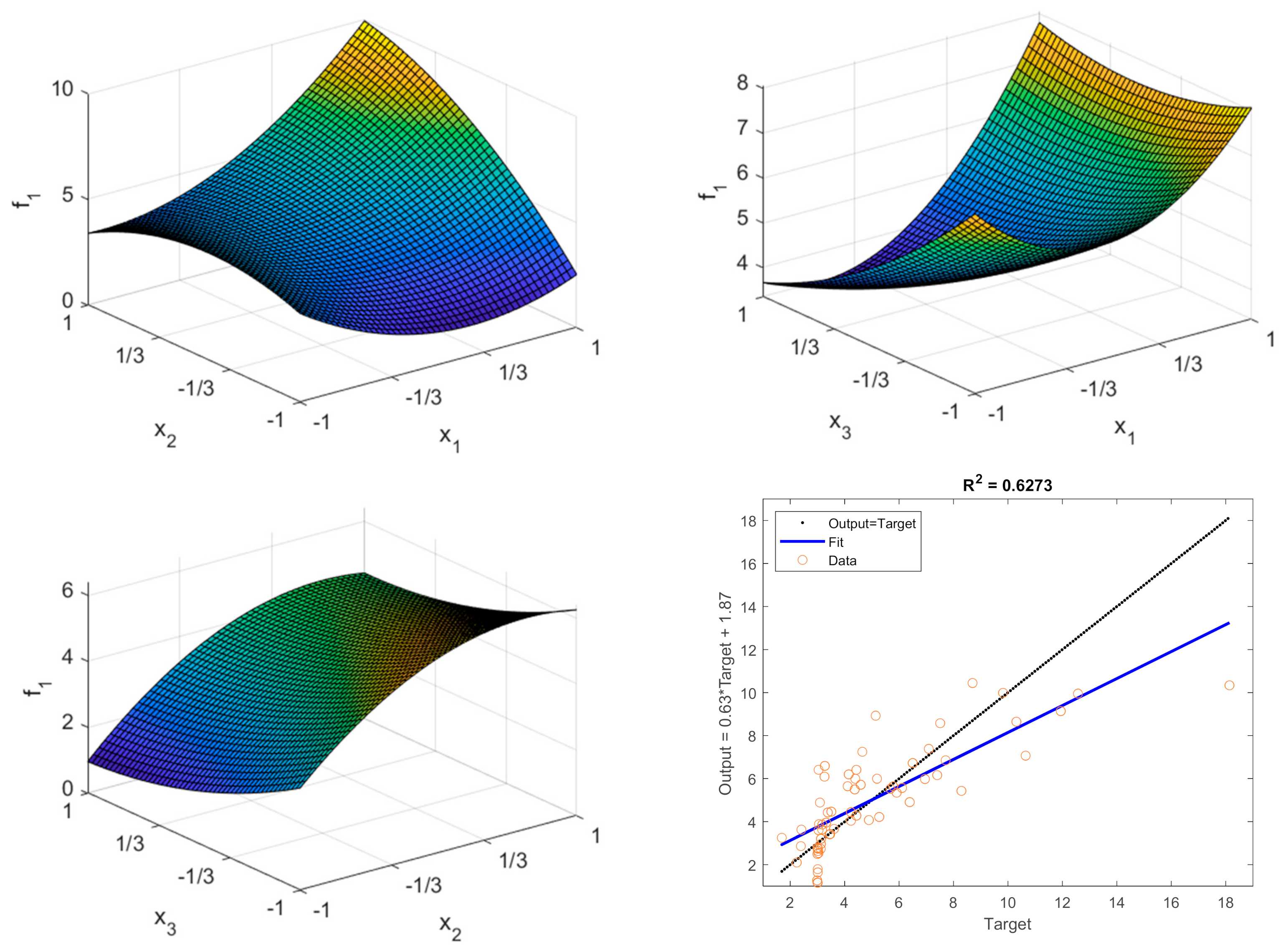
4.1. Regresion Model
Equation (21) shows the regression model that will be first employed to predict the behavior of the output responses obtained from the DOE shown in Table 2. The full regression models will be used instead of those obtained from the higher adj-R2, since the fact of using the model adjusted to the degrees of freedom could eliminate some of the independent variables.
Equation (22) shows that the validation metrics employed in this study are: mean squared error (), root mean squared error (), and mean absolute error (), where are the values provided by the DOE and are the predicted values. As previously mentioned, the model which exhibit the higher coefficient of determination R2 is to be used.
Table 3, Table 4, Table 5 show the obtained results for , , and functions, respectively. As can be observed, regression results are not good enough for and functions and hence these models will not be accurate to predict the behavior of these response variables. On the other hand, the model obtained for function could be used to approximately predict the behavior of this output response which is a relatively simple equation. However, if more accuracy is required, then other models should be used, for example those based on soft computing.
Figure 13 shows the response surface obtained with the regression model of . Because the coefficient of determination of the regression is not very high, the results will not be very reliable with this modeling. Therefore, the fact of considering an optimization using a desirability function with this kind of functions may lead to values with a lack of precision obtained. On the other hand, if it is compared with the actual shape of the real surface of function, which has been shown in Figure 10, the aforementioned can be observed.
Table 4 shows the results obtained for the case of the second function considered in this study. Figure 14 shows the response surface predicted by the regression model. In this case, the function could be used to address the proposed problem since, although the coefficient is not very high, it could give results close to the real optimum of the variable. It may be seen that the shape of the response surface given by the regression model is more similar to the actual shape of the function in this case than in the previous one.
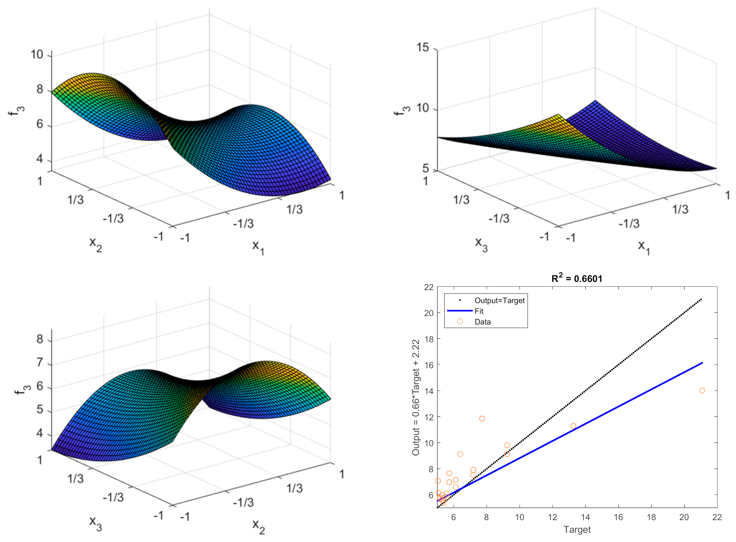
Table 5 shows the results obtained for the case of the third function considered in this study and Figure 15 shows the response surface predicted by the regression model. In this case, as with the first function, the regression model is not able to adequately predict the behavior of the function, which can be observed when comparing the shape of the response surface obtained with the regression model with the actual form of the function, which is shown in Figure 12.
Based on the above, although there are three polynomial models available with which it is possible to use a desirability function and then obtain an optimum, this value will not be precise and it may also occur that this optimum falls outside the limits established in the optimization for some of the variables, as a consequence of the models thus developed; therefore, not having high values of the regression determination coefficients, they will not adequately predict the actual behavior of the response variables.
4.2. Adaptive Neuro Fuzzy Inference System (ANFIS) Modeling
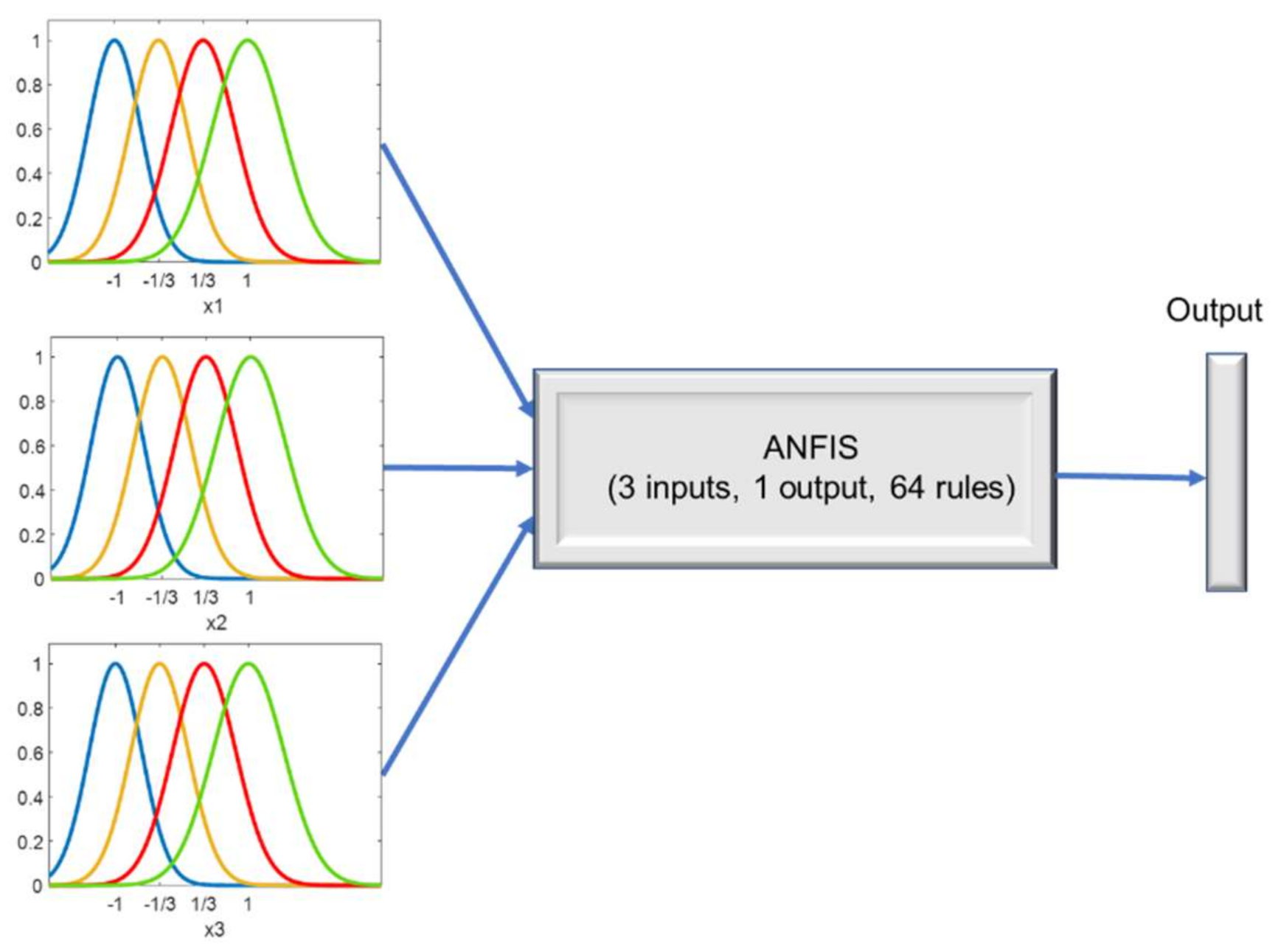
In order to avoid the above-mentioned drawbacks of the regression models, soft computing modeling based for example on artificial neuronal networks (ANNs) could be used. In [61], different types of ANNs are shown. However, in this present study a FIS which is later tuned by using an ANFIS is considered [3]. Specifically, a zero-order Sugeno FIS is employed by using the Fuzzy Logic Toolbox™ of MATLABTM2020a [62], because the de-fuzzification process for a Sugeno system is computationally more efficient compared to that of a Mamdani system [62,63]. However, it should be stated that a Mamdani FIS could have been used. Furthermore, the membership functions for fuzzification of the independent variables are Gaussian as shown in Equation (23). These membership functions have been developed from the methodology shown in [60], although some other membership functions could have been used.
As previously mentioned, in the present study, no additional points will be used to optimize the FIS models as suggested in [60]. It should be noted that if a greater number of data is available to this end, then the ANFIS models obtained will be more reliable. In any case, it can be observed in this section that the models that the ANFIS provide much better results than those obtained with the regression.
The aggregation method is the sum of the fuzzy sets and the aggregated output is obtained from the weighted average of all output rules, where product implication method is used in Sugeno systems [62]. For the rule, the implication method is obtained from Equations (24) and (25) shows the output of the FIS.
The created FIS will have a set of rules of the form
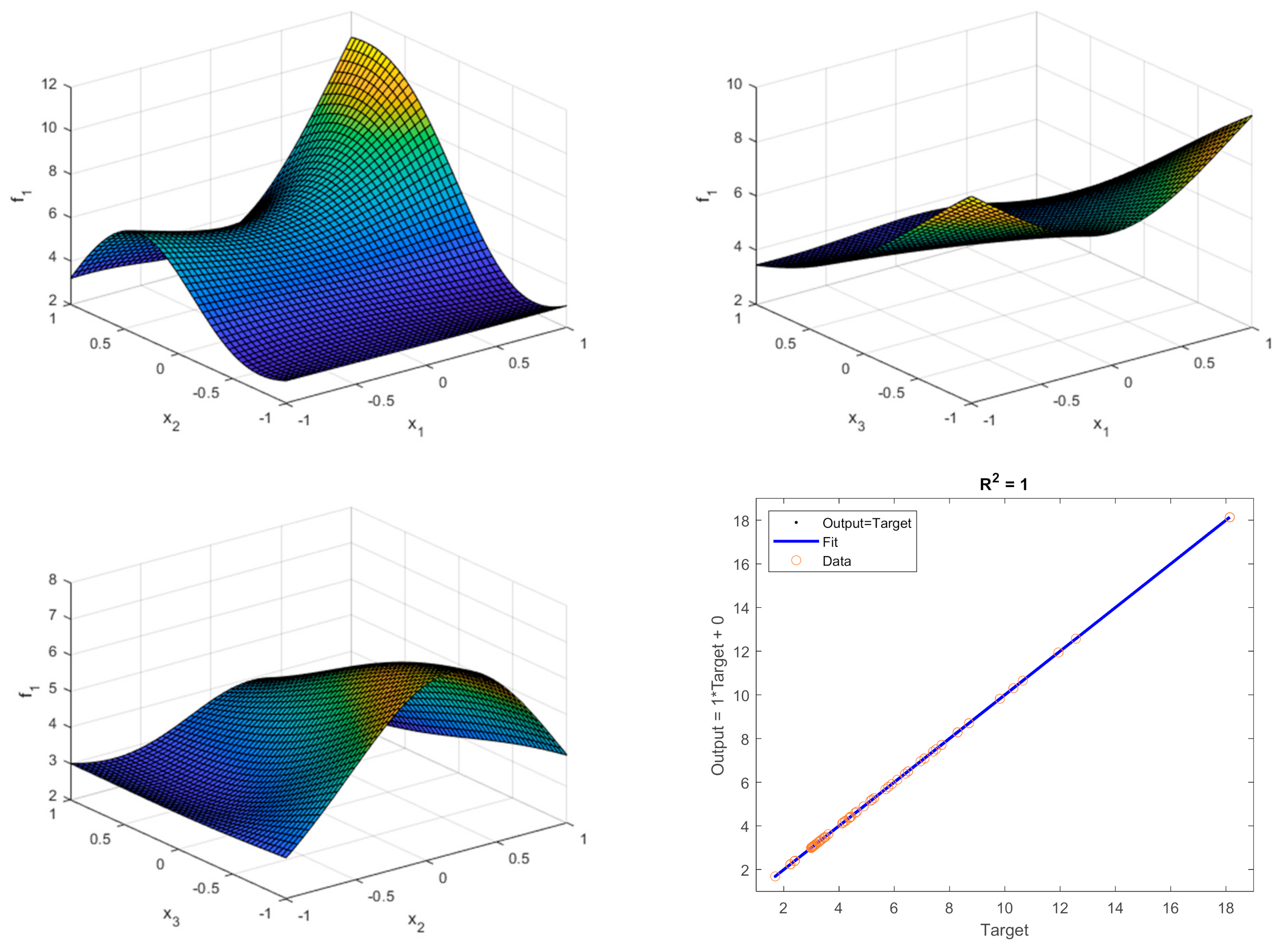
Figure 16 shows the structure of the ANFIS employed in this present study and Figure 17 shows the response surfaces obtained with the ANFIS developed for the first response variable and the values of the statistics employed are shown in Table 6. It can be noted that they are much better than those obtained in the case of the regression for this variable, which were shown in Table 3. Likewise, it can be observed that the ANFIS is capable of adequately predicting the real form of the function despite not having optimized the FIS with additional points.
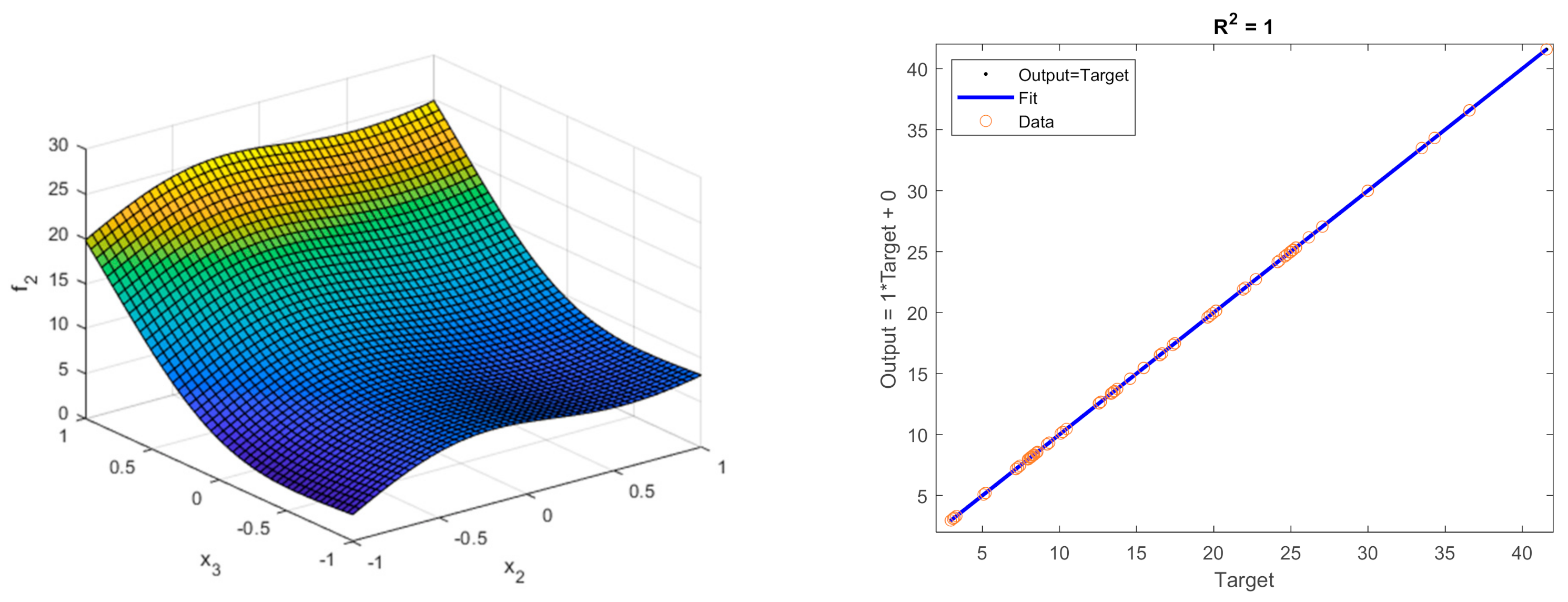
A similar result is obtained for function as can be observed both in Table 7 and in Figure 18. Analogously to the previous case, results obtained with the ANFIS improve very much on those obtained with the regression.
Likewise, Table 8 and Figure 19 show the obtained results with the ANFIS for the case of function. It is observed that this function is now adequately modeled, contrary to that observed with the regression model.
As can be seen in the results obtained in this Section, the precision obtained with the ANFIS models is much higher than that obtained with the regression. Therefore, the prediction developed using ANFIS will be more accurate, especially for regression models not having highly R-squared coefficients. It is worth mentioning the fact that the availability of analytical models, such as those provided by the regression, makes it possible to employ them with optimization algorithms when they are combined with a desirability function. In that way, the desirability function based on the arctangent, which has been shown in Section 3, could be employed to obtain a value that simultaneously optimizes the required conditions by using a desirability function. As previously mentioned, in this case t has to be higher than zero . A value of may be enough, if necessary, it could be reduced. However, if regression models are not accurate it is preferrable either to employ, as an approach, the values obtained directly from the DOE or to employ soft computing techniques. Because, if the regression models are not accurate, it is very likely that the optimization will not be so either. In order to overcome this drawback, the ANFIS models will be employed in order to approach the optimum of the functions by using a desirability function.
4.3. Analysis of the Case Study
In order to compare the results attained, the values obtained with the proposed methodology will be compared with those obtained by using the transformation suggested by Derringer and Suich [18]. The symmetrical DOE shown in Table 2 with three output variables , , and will be used. As previously mentioned, the preferred level of is its minimum, the preferred level of is its maximum and has to be within a set range, defined by a lower bound and by an upper bound. For example, , although this range could be whatever. In order to set the maximum and minimum level of each variable, those provided by the DOE are considered, as shown in Table 9, although they could be any other value.
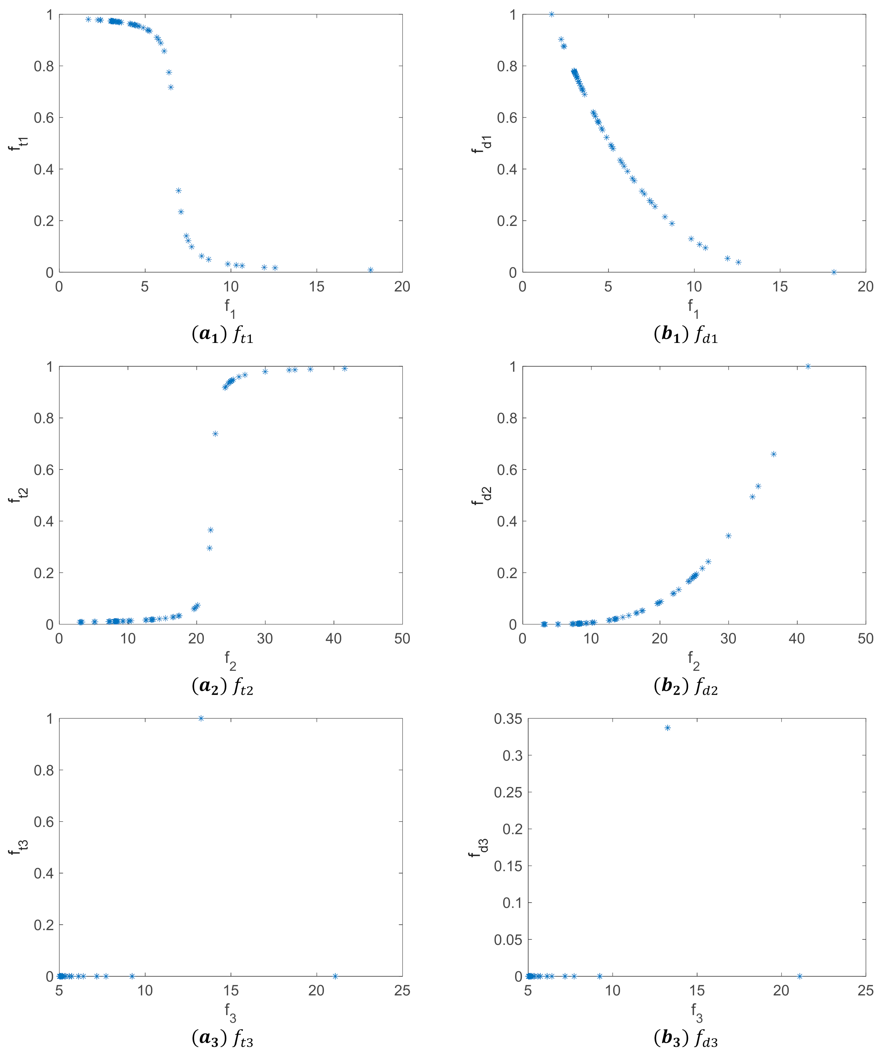
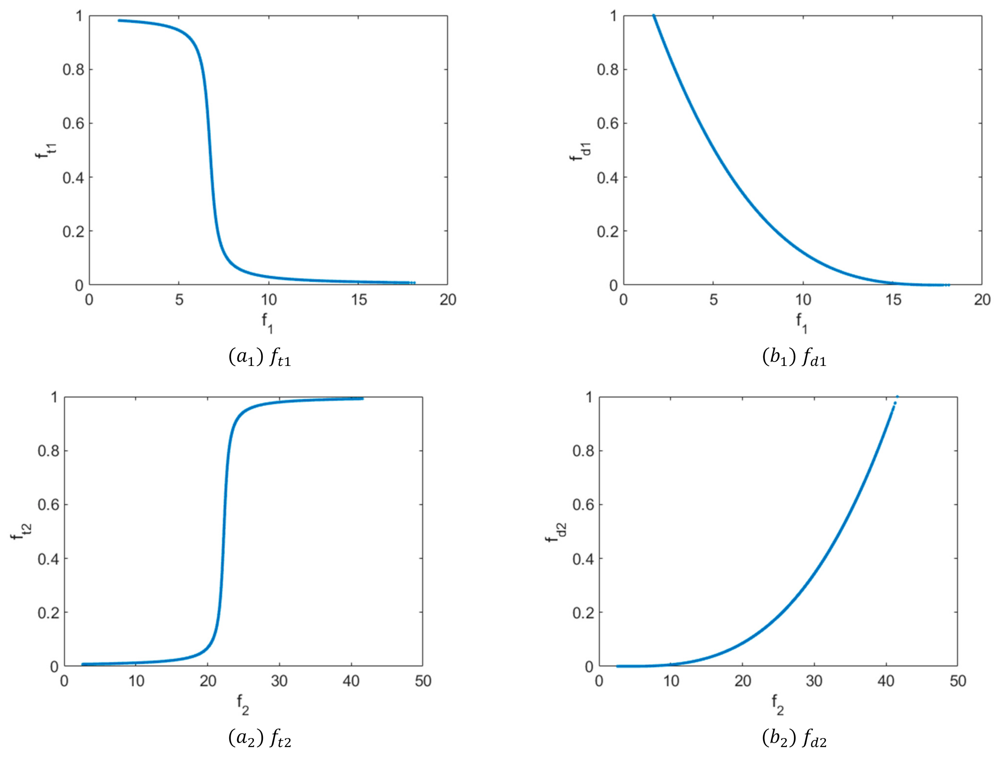
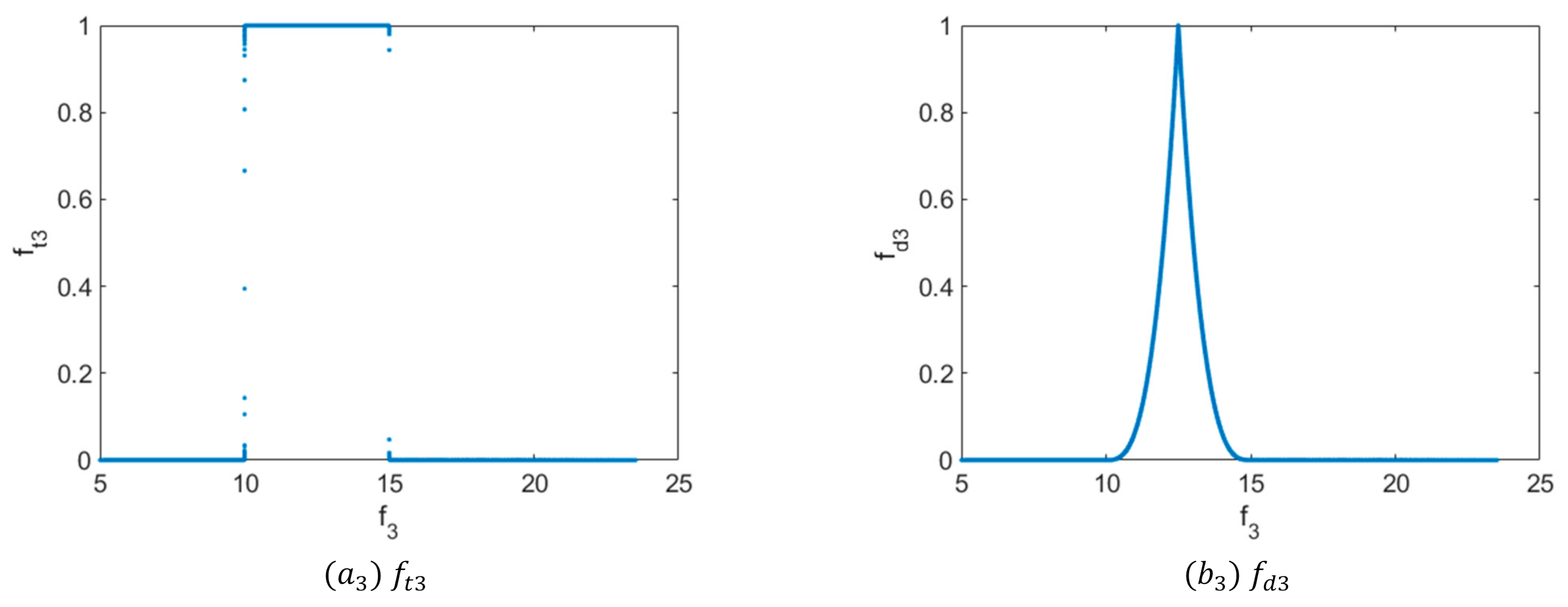
Figure 20b1–b3 show how the data of the output variables obtained from the DOE are classified by using the Derringer and Suich [18] transformation, where it has been considered (r = 3; for one side transformation, s = t = 3, for two-side transformation and c = (LB + UB)/2). Figure 20a1–a3 show these data classified by using the proposed arctangent transformation, in the case of minimizing , maximizing , and in order to keep within a certain range. Table 10 shows the values of the constants to transform the and outputs using the arctangent transformation. Where it was desired to weight the values of . Hence the values shown in this table. On the other hand, to keep within the desired range [LB,UB] = [10,15], where . However, other values could have been used. As can be observed in Table 2 the range of values specified for to stay within only has one output value of this variable although it is obtained in two combinations of the independent variables.
Table 11 shows the optimum values found directly with the data provided by the symmetrical DOE, which is shown in Table 2, where refers to the desirability value obtained with the arctangent transformation and that obtained by using Derringer and Suich [18], both results are obtained by using the non-weighted geometric average. However, it may occur that the DOE does not provide values within a certain range for example, in this case study, within the range [15,20] or that we want to explore the possibility of finding improved values, then if regression results are not accurate, as is the present case, an ANFIS is to be used to overcome this drawback.
It could be possible to define a relative index to compare both desirability functions , ) however this is not carried out in this study. As can be observed in Table 11 the optimal values that both functions find, using only the data provided by the DOE, are the same which is logical as the number of points is not high enough to allow significant differences to exist. In order to employ the ANFIS models, whenever the regression is not accurate enough, first the initial DOE which was employed to develop these ANFIS models, is discretized by using N points. In this study the same number of points has been employed for each of the three independent variables, in order to have an “augmented-symmetrical N3 design of experiments”, although the number of points to discretize each independent variable could be different. From the above, the DOE is discretized as Equation (26) shows. That is, N points are obtained within the range .
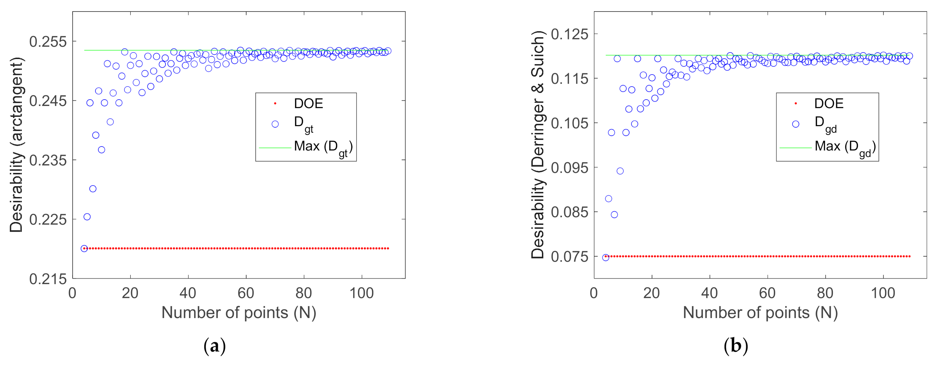
First of all, all combinations of the data provided by Equation (26) are evaluated making use of the previously developed ANFIS models, and hence N3 outputs will be obtained for the response variables, which can be then combined to determine the optimum value of a previously defined parameter, which is, in this present study the geometric mean. This optimum value will be linked to a point, in this case, (,,) withing the selected range and this will be the value that approximate to the optimum of the function. The higher the number of the selected levels, the higher the accuracy of the approach. If N is high enough the approach to the optimum will be accurate. A convergence criterion could be established based, for example, on the convergence band obtained from the optimal values found in each iteration with the desirability functions depending on the number of points (N), among others. However, this is not considered in this study and the optimal values are determined after considering a value of N high enough to observe the convergence of the optimal values that provide the desirability functions in each iteration. Figure 21a,b show the optimal values of the desirability function versus the number of points (N) employed in the ANFIS (in this case combinations of the variables, because there are three independent variables) where is the desirability function obtained by using the geometric mean and the proposed transformation and the desirability values obtained from the geometric mean and the methodology of Derringer and Suich [18]. Moreover, a comparison with the value provided by using the initial data of the DOE can be observed in this figure for both desirability functions when using the ANFIS to generate the values of the output responses. As can be observed, results attained improve those obtained directly with the initial DOE.
Figure 22 show the transformed function by using the ANFIS models both with the proposed desirability function and with that of Derringer and Suich [18].
Table 12 presents the optimal values found with the ANFIS. As can be observed in Table 12, the optimum value with the proposed desirability function is obtained after using N = 55 points, to be evaluated with the ANFIS models, that is (553 combinations of the variables) and it leads to the values of which, in the case of this present study, are improved values, of the response variables, compared with those obtained with Derringer and Suich [18] desirability function (after N = 97 iterations, 973 combinations of the variables evaluated with the ANFIS models),which leads to That is, with the proposed desirability function is more minimized and is more maximized while is kept within the desired range, which may be a consequence of the weighting values employed in the Derringer and Suich [18] transformation, which were fixed at (r = s = t = 3), as previously mentioned. It may occur that other values of this transformation could lead to improved results. Moreover, it is also likely that the attained results with the arctangent may also vary if different constants of those shown in Table 10 were selected. However, this is not analyzed in this present study.
Results obtained with the regression models are shown in Table 13. As can be observed, the results provided by the regression do not fit very well with the actual values of the function and in the case of using the Derringer and Suich [18] desirability function are outside specified tolerances for since the tolerance range specified for this response variable was .
Therefore, as shown in Table 12 and Table 13 results obtained with the ANFIS are more accurate than those provided by using the regression models. Moreover, in the case of using regression models with lack of precision non-desirable results could be obtained as Table 13 shows. Table 14 presents a summary of the results obtained with the Derringer&Suich desirability function [18] and the new proposed desirability function and Table 15 shows the actual values of the functions used to generate the data shown in Table 2.
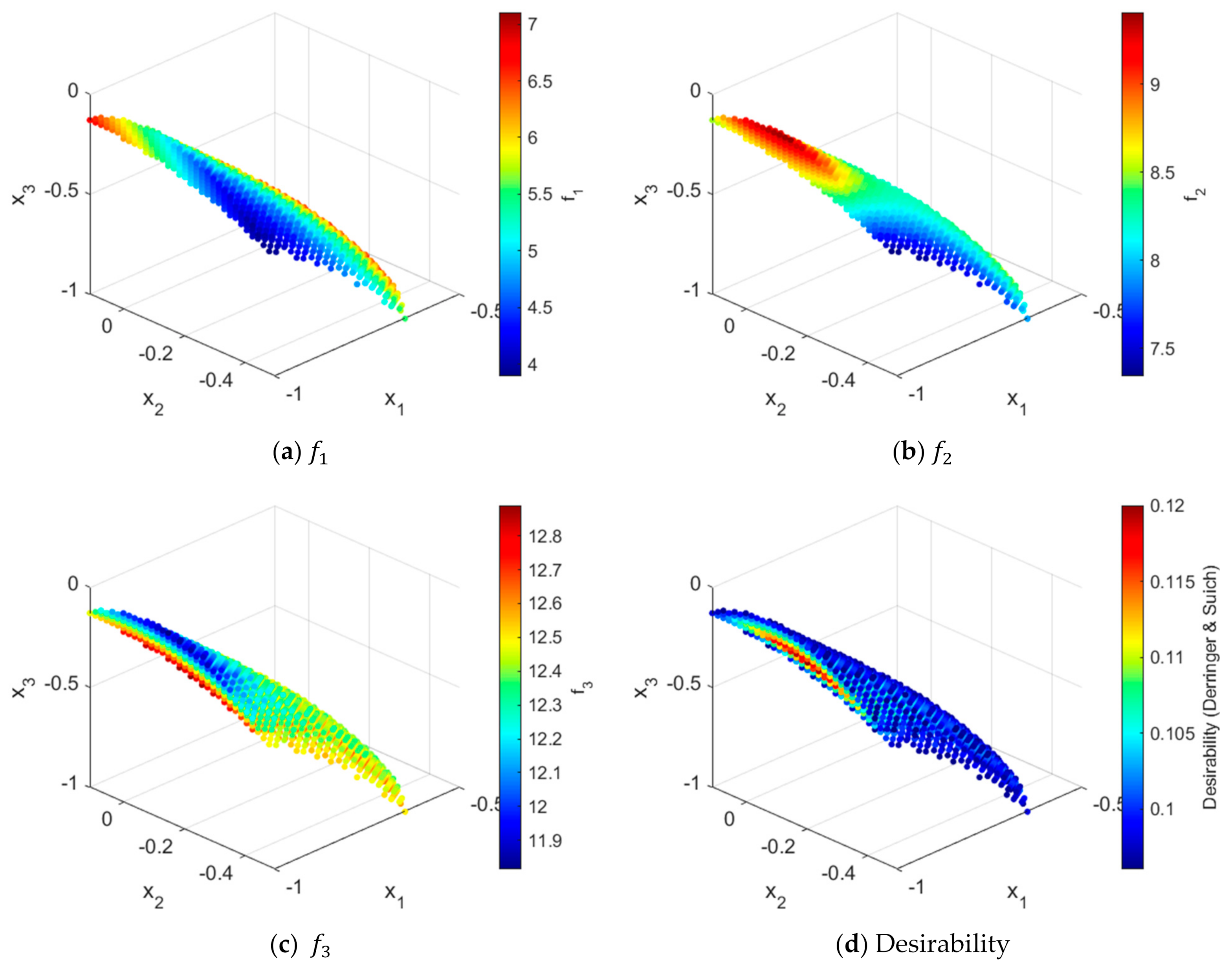
It should be mentioned that in this case study the desirability functions do not provide high values due to the fact that has to be kept within a certain range. Some other combinations could lead to different values being found. For example, Figure 1 shows the values of the proposed arctangent desirability function for a multiple optimization problem where the preferred level of variation of was selected to be the minimum value instead of being fixed within a tolerance range and the maximum was the preferred level for both and . However, it may be that a technological interest exists in maintaining an output response within a certain range while other variables are being simultaneously optimized, and as has been shown in this present study, a design of experiments combined with an ANFIS and a desirability function may obtain an accurate approach to the optimum value even in the event that the DOE does not provide values in a certain range which has to be selected for a variable to be kept within. On the other hand, as can be seen for example in the research study of Derringer [64] it is often observed that when one property improves, it is usually at the expense of others. By using the proposed methodology, it is possible to have all available data attained by the ANFIS, that is, the combination of both independent and dependent variables which lead to a specific desirability value and then allow the user to select the most appropriate combination of the independent variables (process parameters) which lead to reaching a certain value in the response variables. Therefore, it could be possible to establish classes of desirability and several solutions can be obtained instead of a single optimum since it may happen that several combinations of the independent variables may lead to very close values and the fact of selecting the better result could avoid some others being taken into account, which may, in turn, be of technological interest.
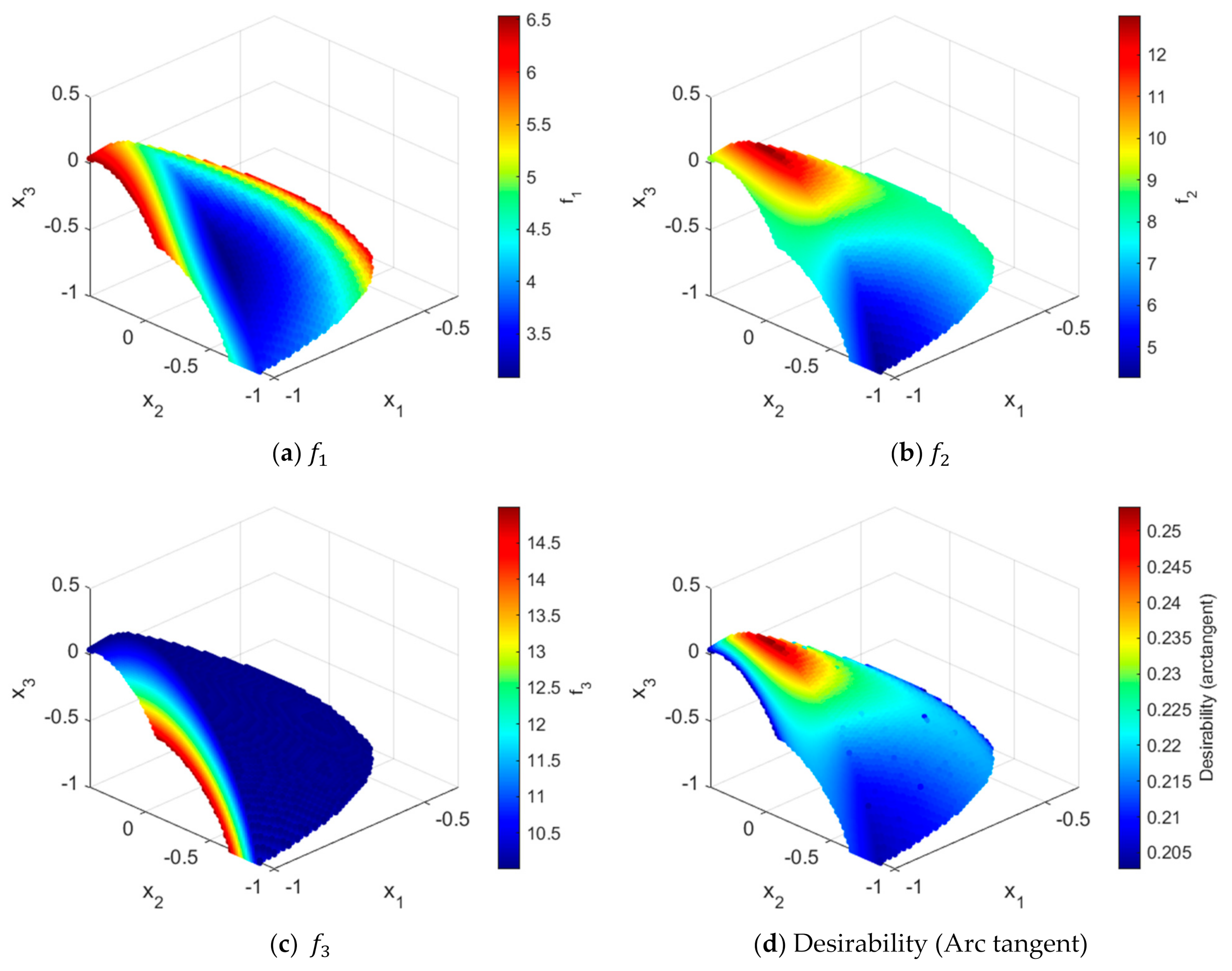
Figure 23a–d and Figure 24a–d show the desirability functions versus the number of variables in both cases examined in this present study as well as the values of the response variables which correspond to a selected level of the desirability function (these figures show the combination of the independent variables that lead to desirability function values being obtained that are higher than 80% of the maximum desirability value of each desirability function respectively). Therefore, it is possible to see the desired levels of the process parameters as well as their influence on the desirability function.
5. Conclusions
This present research study shows a methodology based on using a design of experiments along with an ANFIS and a desirability function for simultaneous multiple response optimization which can be applied to overcome the drawbacks of the regression techniques.
A new desirability function has been proposed and analyzed in this research study. The proposed desirability function is based on the arctangent function and it may adopt several shapes as a function of its parameters.
By using the proposed methodology, it could be possible to establish classes of desirability along with the values of the process parameters and the responses variables and then select the most appropriate ones with higher accuracy than that obtained by conventional regression techniques.
Funding
This research received no external funding.
Institutional Review Board Statement
Not applicable.
Informed Consent Statement
Not applicable.
Conflicts of Interest
The author declares no conflict of interest.
References
- Takagi, T.; Sugeno, M. Fuzzy identification of systems and its applications to modeling and control. IEEE Trans. Syst. Man, Cybern. 1985, SMC-15, 116–132. [Google Scholar] [CrossRef]
- Mamdani, E. Application of fuzzy algorithms for control of simple dynamic plant. Proc. Inst. Electr. Eng. 1974, 121, 1585. [Google Scholar] [CrossRef]
- Jang, J.-S.R. ANFIS: Adaptive-network-based fuzzy inference system. IEEE Trans. Syst. Man Cybern. 1993, 23, 665–685. [Google Scholar] [CrossRef]
- Shihabudheen, K.; Pillai, G. Recent advances in neuro-fuzzy system: A survey. Knowl.-Based Syst. 2018, 152, 136–162. [Google Scholar] [CrossRef]
- Kumar, D.; Karwasra, K.; Soni, G. Bibliometric analysis of artificial neural network applications in materials and engineering. Mater. Today Proc. 2020, 28, 1629–1634. [Google Scholar] [CrossRef]
- Soltanali, H.; Rohani, A.; Abbaspour-Fard, M.H.; Farinha, J.T. A comparative study of statistical and soft computing techniques for reliability prediction of automotive manufacturing. Appl. Soft Comput. 2021, 98, 106738. [Google Scholar] [CrossRef]
- Pandiyan, V.; Caesarendra, W.; Glowacz, A.; Tjahjowidodo, T. Modelling of Material Removal in Abrasive Belt Grinding Process: A Regression Approach. Symmetry 2020, 12, 99. [Google Scholar] [CrossRef] [Green Version]
- Versaci, M. Fuzzy approach and Eddy currents NDT/NDE devices in industrial applications. Electron. Lett. 2016, 52, 943–945. [Google Scholar] [CrossRef]
- Versaci, M.; Calcagno, S.; Cacciola, M.; Morabito, F.C.; Palamara, I.; Pellicanò, D. Innovative Fuzzy Techniques for Characterizing Defects. In Ultrasonic Nondestructive Evaluation; Springer International Publishing: New York, NY, USA, 2015; Chapter 7. [Google Scholar]
- Buntam, D.; Permpoonsinsup, W.; Surin, P. The Application of a Hybrid Model Using Mathematical Optimization and Intelligent Algorithms for Improving the Talc Pellet Manufacturing Process. Symmetry 2020, 12, 1602. [Google Scholar] [CrossRef]
- Gkountakou, F.; Papadopoulos, B. The Use of Fuzzy Linear Regression and ANFIS Methods to Predict the Compressive Strength of Cement. Symmetry 2020, 12, 1295. [Google Scholar] [CrossRef]
- Shah, H.; Gopal, M. A Reinforcement Learning Algorithm with Evolving Fuzzy Neural Networks. IFAC Proc. Vol. 2014, 47, 1161–1165. [Google Scholar] [CrossRef] [Green Version]
- Hrehova, S.; Mizakova, J. Evaluation a Process using Fuzzy Principles and Tools of Matlab. Int. J. Appl. Math. Comput. Sci. Syst. Eng. 2019, 1, 61–65. [Google Scholar]
- Makarenko, A. Multiple-Valued and Branching Neural Networks. In Proceedings of the 2019 International Joint Conference on Neural Networks (IJCNN), Budapest, Hungary, 14–19 July 2019. [Google Scholar]
- Bose, M. The mathematics of symmetrical factorial designs. Resonance 2003, 8, 14–19. [Google Scholar] [CrossRef]
- Shirakura, T. Fractional factorial designs of two and three levels. Discret. Math. 1993, 116, 99–135. [Google Scholar] [CrossRef] [Green Version]
- Harrington, E.C. The Desirability Function. Ind. Qual. Control. 1965, 21, 494–498. [Google Scholar]
- Derringer, G.; Suich, R. Simultaneous Optimization of Several Response Variables. J. Qual. Technol. 1980, 12, 214–219. [Google Scholar] [CrossRef]
- Del Castillo, E.; Montgomery, D.C.; McCarville, D.R. Modified Desirability Functions for Multiple Response Optimization. J. Qual. Technol. 1996, 28, 337–345. [Google Scholar] [CrossRef]
- He, Z.; Zhu, P.F. A hybrid genetic algorithm for multiresponse parameter optimization within desirability function framework. In Proceedings of the 2010 IEEE International Conference on Industrial Engineering and Engineering Management, Beijing, China, 21–23 October 2009; Institute of Electrical and Electronics Engineers (IEEE); pp. 612–617. [Google Scholar]
- Costa, N.R.; Lourenço, J.; Pereira, Z.L. Desirability function approach: A review and performance evaluation in adverse conditions. Chemom. Intell. Lab. Syst. 2011, 107, 234–244. [Google Scholar] [CrossRef]
- Kim, K.; Lin, D.K.J. Simultaneous optimization of mechanical properties of steel by maximizing exponential desirability functions. J. R. Stat. Soc. Ser. C (Appl. Stat.) 2000, 49, 311–325. [Google Scholar] [CrossRef]
- Kros, J.F.; Mastrangelo, C.M. Comparing Multi-response Design Methods with Mixed Responses. Qual. Reliab. Eng. Int. 2004, 20, 527–539. [Google Scholar] [CrossRef]
- Das, P.; Mukherjee, S.; Ganguly, S.; Bhattacharyay, B.; Datta, S. Genetic algorithm based optimization for multi-physical properties of HSLA steel through hybridization of neural network and desirability function. Comput. Mater. Sci. 2009, 45, 104–110. [Google Scholar] [CrossRef]
- Zhiyu, Z.; Zhen, H.; Xiangfen, K. A new desirability function based method for multi-response robust parameter design. In Proceedings of the International Technology and Innovation Conference 2006 (ITIC 2006), Hangzhou, China, 6–7 November 2006; pp. 178–183. [Google Scholar]
- He, Z.; Zhu, P.-F.; Park, S.-H. A robust desirability function method for multi-response surface optimization considering model uncertainty. Eur. J. Oper. Res. 2012, 221, 241–247. [Google Scholar] [CrossRef]
- Ribardo, C.; Allen, T.T. An alternative desirability function for achieving ?six sigma? quality. Qual. Reliab. Eng. Int. 2003, 19, 227–240. [Google Scholar] [CrossRef]
- Wu, F.-C.; Chyu, C.-C. Optimization of robust design for multiple quality characteristics. Int. J. Prod. Res. 2004, 42, 337–354. [Google Scholar] [CrossRef]
- Ortiz, F., Jr.; Simpson, J.R.; Pignatiello, J.J., Jr.; Heredia-Langner, A. A Genetic Algorithm Approach to Multiple-Response Optimization. J. Qual. Technol. 2004, 36, 432–450. [Google Scholar] [CrossRef]
- Pasandideh, S.H.R.; Niaki, S.T.A. Multi-response simulation optimization using genetic algorithm within desirability function framework. Appl. Math. Comput. 2006, 175, 366–382. [Google Scholar] [CrossRef]
- Das, P. Hybridization of Artificial Neural Network Using Desirability Functions for Process. Int. J. Qual. Res. 2010, 4, 37–50. Available online: http://www.ijqr.net/paper.php?id=156 (accessed on 9 April 2021).
- Lee, M.-S.; Kim, K.-J. Expected Desirability Function: Consideration of Both Location and Dispersion Effects in Desirability Function Approach. Qual. Technol. Quant. Manag. 2007, 4, 365–377. [Google Scholar] [CrossRef]
- He, Z.; Wang, J.; Oh, J.; Park, S.H. Robust optimization for multiple responses using response surface methodology. Appl. Stoch. Model. Bus. Ind. 2010, 26, 157–171. [Google Scholar] [CrossRef]
- Lee, D.-H.; Jeong, I.-J.; Kim, K.-J. A desirability function method for optimizing mean and variability of multiple responses using a posterior preference articulation approach. Qual. Reliab. Eng. Int. 2018, 34, 360–376. [Google Scholar] [CrossRef]
- Fuller, D.; Scherer, W. The desirability function: Underlying assumptions and application implications. In SMC’98 Conference Proceedings. Proceedings of the 1998 IEEE International Conference on Systems, Man, and Cybernetics (Cat.No.98CH36218),San Diego, CA, USA, 14 October 1998; Institute of Electrical and Electronics Engineers (IEEE): New York, NY, USA, 2002; Volume 4, pp. 4016–4021. [Google Scholar]
- Candioti, L.V.; De Zan, M.M.; Cámara, M.S.; Goicoechea, H.C. Experimental design and multiple response optimization. Using the desirability function in analytical methods development. Talanta 2014, 124, 123–138. [Google Scholar] [CrossRef] [PubMed]
- Padilla-Atondo, J.; Limon-Romero, J.; Perez-Sanchez, A.; Tlapa, D.; Baez-Lopez, Y.; Puente, C.; Ontiveros, S. The Impact of Hydrogen on a Stationary Gasoline-Based Engine through Multi-Response Optimization: A Desirability Function Approach. Sustainability 2021, 13, 1385. [Google Scholar] [CrossRef]
- Hur, D.-J.; Jeong, S.-H.; Song, S.-I.; Noh, J.-H. Optimization Based on Product and Desirability Functions for Flow Distribution in Multi-Channel Cooling Systems of Power Inverters in Electric Vehicles. Appl. Sci. 2019, 9, 4844. [Google Scholar] [CrossRef] [Green Version]
- Saleem, M.M.; Farooq, U.; Izhar, U.; Khan, U.S. Multi-Response Optimization of Electrothermal Micromirror Using Desirability Function-Based Response Surface Methodology. Micromachines 2017, 8, 107. [Google Scholar] [CrossRef] [Green Version]
- Akçay, H.; Anagün, A.S. Multi Response Optimization Application on a Manufacturing Factory. Math. Comput. Appl. 2013, 18, 531–538. [Google Scholar] [CrossRef]
- Jumare, A.I.; Abou-El-Hossein, K.; Abdulkadir, L.N.; Liman, M.M. Predictive modeling and multiobjective optimization of diamond turning process of single-crystal silicon using RSM and desirability function approach. Int. J. Adv. Manuf. Technol. 2019, 103, 4205–4220. [Google Scholar] [CrossRef]
- Chahal, M.; Singh, V.; Garg, R. Optimum surface roughness evaluation of dies steel H-11 with CNC milling using RSM with desirability function. Int. J. Syst. Assur. Eng. Manag. 2017, 8, 432–444. [Google Scholar] [CrossRef]
- Zhao, D.; Bezgans, Y.; Vdonin, N.; Du, W. The use of TOPSIS-based-desirability function approach to optimize the balances among mechanical performances, energy consumption, and production efficiency of the arc welding process. Int. J. Adv. Manuf. Technol. 2021, 112, 3545–3559. [Google Scholar] [CrossRef]
- Kribes, N.; Hessainia, Z.; Yallese, M.A. Optimisation of Machining Parameters in Hard Turning by Desirability Function Analysis Using Response Surface Methodology. In Advances in Mechanical Engineering; Metzler, J.B., Ed.; Springer: New York, NY, USA, 2015; Volume 789, pp. 73–81. [Google Scholar]
- Ahmad, A.; Lajis, M.A.; Yusuf, N.K.; Ab Rahim, S.N. Statistical Optimization by the Response Surface Methodology of Direct Recycled Aluminum-Alumina Metal Matrix Composite (MMC-AlR) Employing the Metal Forming Process. Processes 2020, 8, 805. [Google Scholar] [CrossRef]
- Qazi, M.; Abas, M.; Khan, R.; Saleem, W.; Pruncu, C.; Omair, M. Experimental Investigation and Multi-Response Optimization of Machinability of AA5005H34 Using Composite Desirability Coupled with PCA. Metals 2021, 11, 235. [Google Scholar] [CrossRef]
- Osman, N.; Sajuri, Z.; Baghdadi, A.H.; Omar, M.Z. Effect of Process Parameters on Interfacial Bonding Properties of Aluminium–Copper Clad Sheet Processed by Multi-Pass Friction Stir-Welding Technique. Metals 2019, 9, 1159. [Google Scholar] [CrossRef] [Green Version]
- Laghari, R.A.; Li, J.; Mia, M. Effects of Turning Parameters and Parametric Optimization of the Cutting Forces in Machining SiCp/Al 45 wt% Composite. Metals 2020, 10, 840. [Google Scholar] [CrossRef]
- Pradhan, S.; Singh, G.; Bhagi, L.K. Study on surface roughness in machining of Al/SiCp metal matrix composite using desirability function analysis approach. Mater. Today Proc. 2018, 5, 28108–28116. [Google Scholar] [CrossRef]
- Sahoo, D.K.; Mohanty, B.S.; John, D.F.; Pradeep, A.M. Multi response optimization and desirability function analysis on friction surfaced deposition of AISI 316 stainless steel over EN8 medium carbon steel. Mater. Today Proc. 2021, 40, S1–S9. [Google Scholar] [CrossRef]
- Du, F.; He, L.; Huang, H.; Zhou, T.; Wu, J. Analysis and Multi-Objective Optimization for Reducing Energy Consumption and Improving Surface Quality during Dry Machining of 304 Stainless Steel. Materials 2020, 13, 4693. [Google Scholar] [CrossRef] [PubMed]
- Mostafaei, M. ANFIS models for prediction of biodiesel fuels cetane number using desirability function. Fuel 2018, 216, 665–672. [Google Scholar] [CrossRef]
- Labidi, A.; Tebassi, H.; Belhadi, S.; Khettabi, R.; Yallese, M.A. Cutting Conditions Modeling and Optimization in Hard Turning Using RSM, ANN and Desirability Function. J. Fail. Anal. Prev. 2018, 18, 1017–1033. [Google Scholar] [CrossRef]
- Sengottuvel, P.; Satishkumar, S.; Dinakaran, D. Optimization of Multiple Characteristics of EDM Parameters Based on Desirability Approach and Fuzzy Modeling. Procedia Eng. 2013, 64, 1069–1078. [Google Scholar] [CrossRef] [Green Version]
- Singh, A.; Datta, S.; Mahapatra, S.S.; Singha, T.; Majumdar, G. Optimization of bead geometry of submerged arc weld using fuzzy based desirability function approach. J. Intell. Manuf. 2013, 24, 35–44. [Google Scholar] [CrossRef]
- Paschoalinoto, N.W.; Batalha, G.F.; Bordinassi, E.C.; Ferrer, J.A.G.; Filho, A.F.D.L.; Ribeiro, G.D.L.X.; Cardoso, C. MQL Strategies Applied in Ti-6Al-4V Alloy Milling—Comparative Analysis between Experimental Design and Artificial Neural Networks. Materials 2020, 13, 3828. [Google Scholar] [CrossRef]
- Tank, K.; Shetty, N.; Panchal, G.; Tukrel, A. Optimization of turning parameters for the finest surface roughness characteristics using desirability function analysis coupled with fuzzy methodology and ANOVA. Mater. Today Proc. 2018, 5, 13015–13024. [Google Scholar] [CrossRef]
- Salmasnia, A.; Kazemzadeh, R.B.; Tabrizi, M.M. A novel approach for optimization of correlated multiple responses based on desirability function and fuzzy logics. Neurocomputing 2012, 91, 56–66. [Google Scholar] [CrossRef]
- Gajera, H.M.; Dave, K.G.; Darji, V.P.; Abhishek, K. Optimization of process parameters of direct metal laser sintering process using fuzzy-based desirability function approach. J. Braz. Soc. Mech. Sci. Eng. 2019, 41, 124. [Google Scholar] [CrossRef]
- Pérez, C.J.L. A Proposal of an Adaptive Neuro-Fuzzy Inference System for Modeling Experimental Data in Manufacturing Engineering. Mathematics 2020, 8, 1390. [Google Scholar] [CrossRef]
- Beale, M.H.; Hagan, M.T.; Demuth, H.B. Deep Learning ToolboxTMUser’s Guide; The Mathworks Inc.: Herborn, MA, USA, 2018. [Google Scholar]
- The MathWorks Inc. Fuzzy Logic ToolboxTM User’s Guide; The MathWorks Inc.: Portola Valley, CA, USA, 2020. [Google Scholar]
- Burrascano, P.; Callegari, S.; Montisci, A.; Ricci, M.; Versaci, M. Standard Soft Computing Techniques for Characterization of Defects in Nondestructive Evaluation. In Ultrasonic Nondestructive Evaluation Systems, Industrial Application Issues; Springer International Publishing: New York, NY, USA, 2015; Chapter 6; pp. 175–199. [Google Scholar]
- Derringer, G. A balancing act: Optimizing a product’s properties. Qual. Prog. 1994, 27, 51–58. [Google Scholar]
Figure 1.
Desirability function results using a symmetrical design of experiments (DOE) and an ANFIS.
Figure 1.
Desirability function results using a symmetrical design of experiments (DOE) and an ANFIS.

Figure 2.
Influence of constants over the arctangent transformation (a) to maximize an output response and (b) to minimize an output response.
Figure 2.
Influence of constants over the arctangent transformation (a) to maximize an output response and (b) to minimize an output response.

Figure 3.
Influence of constants of the arctangent transformation (a) to maximize an output response, and (b) to minimize an output response.
Figure 3.
Influence of constants of the arctangent transformation (a) to maximize an output response, and (b) to minimize an output response.

Figure 4.
Influence of constants of the arctangent transformation (a) to maximize an output response, and (b) to minimize an output response.
Figure 4.
Influence of constants of the arctangent transformation (a) to maximize an output response, and (b) to minimize an output response.

Figure 5.
Arctangent transformation to (a) maximize a variable, (b) minimize a variable.

Figure 6.
Arctangent transformation to keep a variable in a range (LB = Lower Bound, UB = Upper Bound).
Figure 6.
Arctangent transformation to keep a variable in a range (LB = Lower Bound, UB = Upper Bound).

Figure 7.
Arctangent transformation to (a) maximize a variable, where the value of and to (b) minimize a variable, where the value .
Figure 7.
Arctangent transformation to (a) maximize a variable, where the value of and to (b) minimize a variable, where the value .

Figure 8.
Arctangent transformation to keep a variable in a range (LB = Lower Bound; UB = Upper Bound).
Figure 8.
Arctangent transformation to keep a variable in a range (LB = Lower Bound; UB = Upper Bound).

Figure 9.
Arctangent transformation to (left) maximize a variable and (right) minimize a variable by selecting the levels of transition to “0” and “1”, where and and and and . In the case shown in the figure the same values have been selected , .
Figure 9.
Arctangent transformation to (left) maximize a variable and (right) minimize a variable by selecting the levels of transition to “0” and “1”, where and and and and . In the case shown in the figure the same values have been selected , .

Figure 10.
Actual shape of function.

Figure 11.
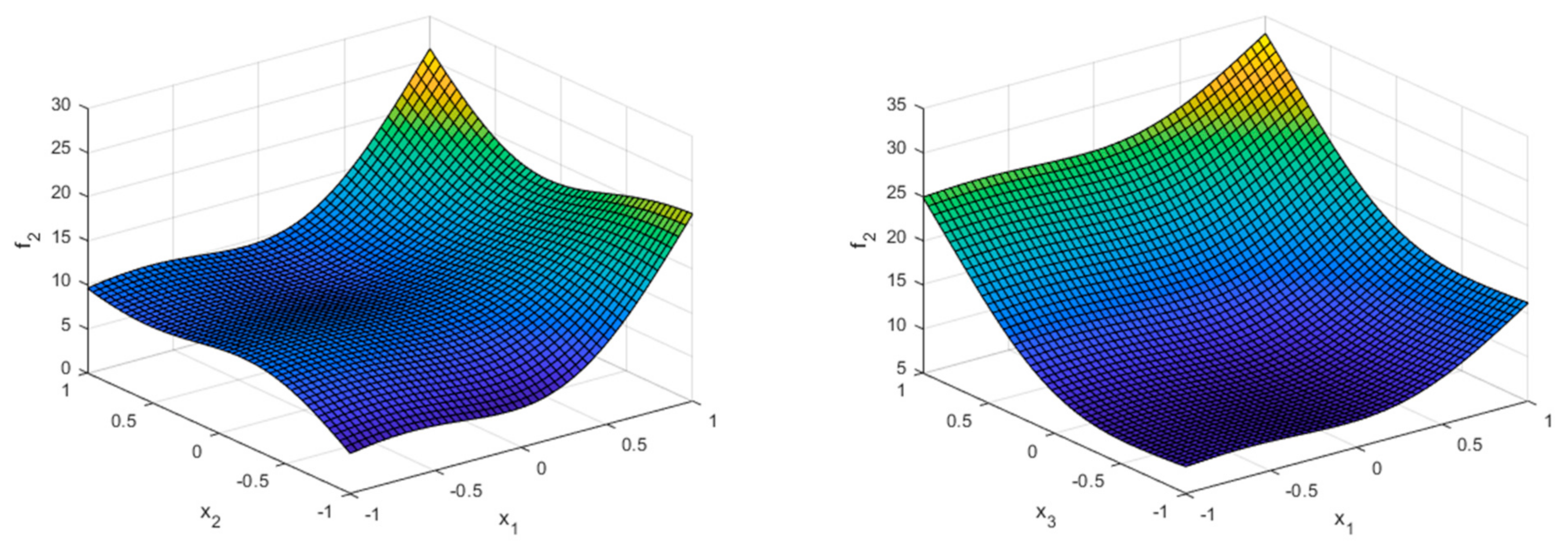
Actual shape of function.

Figure 12.
Actual shape of function.

Figure 13.
Response surface of obtained with the regression model.

Figure 14.
Response surface of obtained with the regression model.

Figure 15.
Response surface of obtained with the regression model.

Figure 16.
Adaptive neuro-fuzzy inference system (ANFIS).

Figure 17.
Response surface of obtained with the ANFIS model.

Figure 18.
Response surface of obtained with the ANFIS model.


Figure 19.
Response surface of obtained with the ANFIS model.

Figure 20.
Score of the response variables of the DOE using the arctangent transformation (sub index “t”) and that proposed by Derringer and Suich [18] (sub index “d”).
Figure 20.
Score of the response variables of the DOE using the arctangent transformation (sub index “t”) and that proposed by Derringer and Suich [18] (sub index “d”).

Figure 21.
Desirability functions versus the number of points (N) employed in the ANFIS.

Figure 22.
Transformation of the values of the response functions obtained by using the ANFIS (a1–a3) Using the proposed desirability function and (b1–b3) using the Derringer and Suich [18] desirability function.
Figure 22.
Transformation of the values of the response functions obtained by using the ANFIS (a1–a3) Using the proposed desirability function and (b1–b3) using the Derringer and Suich [18] desirability function.


Figure 23.
Derringer and Suich [18] desirability function and response variables versus the independent variables, using the ANFIS (only values within 80–100% of the maximum desirability value obtained with the Derringer and Suich desirability function () have been plotted).
Figure 23.
Derringer and Suich [18] desirability function and response variables versus the independent variables, using the ANFIS (only values within 80–100% of the maximum desirability value obtained with the Derringer and Suich desirability function () have been plotted).

Figure 24.
Proposed desirability function and response variables versus the independent variables, using the ANFIS (only values within 80–100% of the maximum desirability value obtained with the proposed desirability function () have been plotted).
Figure 24.
Proposed desirability function and response variables versus the independent variables, using the ANFIS (only values within 80–100% of the maximum desirability value obtained with the proposed desirability function () have been plotted).


Table 1.
Factors and levels of the symmetrical DOE.
| Design Factors | Levels and Values | |||
|---|---|---|---|---|
| −1 | −1/3 | 1/3 | 1 | |
| −1 | −1/3 | 1/3 | 1 | |
| −1 | −1/3 | 1/3 | 1 | |
Table 2.
Values of the dependent variables using a symmetrical DOE.
| Exp. | Exp. | Exp. | Exp. | ||||||||||||
|---|---|---|---|---|---|---|---|---|---|---|---|---|---|---|---|
| 1 | 3.27 | 3.10 | 7.72 | 17 | 3.18 | 3.32 | 5.72 | 33 | 3.12 | 5.21 | 5.19 | 49 | 3.13 | 19.74 | 5.05 |
| 2 | 3.09 | 2.96 | 6.40 | 18 | 3.04 | 3.19 | 5.37 | 34 | 3.01 | 5.08 | 5.10 | 50 | 3.02 | 19.60 | 5.03 |
| 3 | 3.04 | 8.34 | 5.72 | 19 | 3.01 | 8.57 | 5.19 | 35 | 2.99 | 10.46 | 5.05 | 51 | 3.00 | 24.98 | 5.01 |
| 4 | 3.02 | 19.93 | 5.37 | 20 | 3.01 | 20.15 | 5.10 | 36 | 3.00 | 22.04 | 5.03 | 52 | 3.00 | 36.57 | 5.01 |
| 5 | 7.09 | 8.14 | 21.08 | 21 | 6.11 | 8.27 | 9.24 | 37 | 5.91 | 9.33 | 6.12 | 53 | 6.50 | 17.48 | 5.29 |
| 6 | 4.59 | 8.01 | 13.26 | 22 | 4.43 | 8.13 | 7.18 | 38 | 4.23 | 9.20 | 5.57 | 54 | 4.15 | 17.35 | 5.15 |
| 7 | 3.51 | 13.39 | 9.24 | 23 | 3.45 | 13.51 | 6.12 | 39 | 3.32 | 14.58 | 5.29 | 55 | 3.26 | 22.73 | 5.08 |
| 8 | 3.17 | 24.97 | 7.18 | 24 | 3.13 | 25.10 | 5.57 | 40 | 3.06 | 26.16 | 5.15 | 56 | 3.04 | 34.31 | 5.04 |
| 9 | 10.65 | 7.31 | 21.08 | 25 | 7.40 | 7.44 | 9.24 | 41 | 7.71 | 8.50 | 6.12 | 57 | 11.94 | 16.65 | 5.29 |
| 10 | 8.29 | 7.18 | 13.26 | 26 | 6.39 | 7.30 | 7.18 | 42 | 6.95 | 8.36 | 5.57 | 58 | 10.31 | 16.51 | 5.15 |
| 11 | 5.27 | 12.56 | 9.24 | 27 | 4.89 | 12.68 | 6.12 | 43 | 5.68 | 13.74 | 5.29 | 59 | 7.51 | 21.89 | 5.08 |
| 12 | 3.47 | 24.14 | 7.18 | 28 | 3.61 | 24.26 | 5.57 | 44 | 4.37 | 25.33 | 5.15 | 60 | 5.14 | 33.48 | 5.04 |
| 13 | 5.78 | 8.10 | 7.72 | 29 | 4.11 | 8.32 | 5.72 | 45 | 4.65 | 10.21 | 5.19 | 61 | 8.70 | 24.74 | 5.05 |
| 14 | 4.23 | 7.96 | 6.40 | 30 | 3.38 | 8.19 | 5.37 | 46 | 4.43 | 10.08 | 5.10 | 62 | 9.82 | 24.60 | 5.03 |
| 15 | 2.39 | 13.34 | 5.72 | 31 | 2.41 | 13.57 | 5.19 | 47 | 4.39 | 15.46 | 5.05 | 63 | 12.57 | 29.98 | 5.01 |
| 16 | 2.24 | 24.93 | 5.37 | 32 | 1.69 | 25.15 | 5.10 | 48 | 5.19 | 27.04 | 5.03 | 64 | 18.14 | 41.57 | 5.01 |
Table 3.
Regression results for the first output response.
| Regression | 0.6273 | 1.7893 | 3.2015 | 1.2549 |
Table 4.
Regression results for the second output response.
| Regression | 0.9523 | 1.9817 | 3.9273 | 1.6819 |
Table 5.
Regression results for the third output response.
| Regression | 0.6601 | 1.8221 | 3.3201 | 1.2238 |
Table 6.
ANFIS results for the first output response.
| ANFIS | 1.0000 | 0.0050 | 2.4881 × 10⁻⁵ | 0.0039 |
Table 7.
ANFIS results for the second output response.
| ANFIS | 1.0000 | 7.9133 × 10⁻⁴ | 6.2621 × 10⁻⁷ | 6.5990 × 10⁻⁴ |
Table 8.
ANFIS results for the third output response.
| ANFIS | 1.0000 | 0.0038 | 1.4506 × 10⁻⁵ | 0.0033 |
Table 9.
Ranges of the output responses.
| Function | Min | Max |
|---|---|---|
| 1.69 | 18.14 | |
| 2.96 | 41.57 | |
| 5.01 | 21.08 |
Table 10.
Values of the constants to transform the and outputs.
| Function | Desired Level | |||||
| Max. | 2 | 0.2 | 1 | 1.69 | 18.14 | |
| Min. | 1 | 0.5 | 1 | 2.96 | 41.57 |
Table 11.
Desirability values obtained from the DOE.
| Exp. | |||||||
| 6 | 0.2201 | −1 | −1/3 | −1/3 | 4.59 | 8.01 | 13.26 |
| Exp. | |||||||
| 6 | 0.0750 | −1 | −1/3 | −1/3 | 4.59 | 8.01 | 13.26 |
Table 12.
Results attained with the ANFIS models and the desirability functions.
| Arctangent | |||||||
| Num. Points: 55 | 0.2535 | −1.0000 | −0.0526 | 0.2982 | 4.5892 | 12.9599 | 10.0063 |
| Actual values (i.e., obtained with the actual functions) | 4.2857 | 11.6280 | 10.4535 | ||||
| Derringer & Suich | |||||||
| Num. Points: 97 | 0.1202 | −1.0000 | −0.2121 | −0.1717 | 4.9343 | 8.7416 | 12.5005 |
| Actual values (i.e., obtained with the actual functions) | 4.8071 | 8.1795 | 13.0183 | ||||
Table 13.
Results attained with the regression models and the desirability functions.
| Arctangent | ||||||
| Regression Results | −1.0000 | 0.1489 | 0.1064 | 4.7649 | 10.2241 | 10.0073 |
| Actual values (i.e., obtained with the actual functions) | 5.7264 | 9.2598 | 11.3551 | |||
| Derringer & Suich | ||||||
| Regression Results | −1.0000 | 0.8571 | −1.0000 | 6.0402 | 8.9376 | 12.4994 |
| Actual values (i.e., obtained with the actual functions) | 7.0248 | 8.1123 | 9.6217 | |||
Table 14.
Comparison of the results obtained.
| Derringer & Suich | ANFIS | 4.9343 | 8.7416 | 12.5005 |
| Regression | 6.0402 | 8.9376 | 12.4994 | |
| Arctangent | ANFIS | 4.5892 | 12.9599 | 10.0063 |
| Regression | 4.7649 | 10.2241 | 10.0073 |
Table 15.
Actual values of and functions.
Publisher’s Note: MDPI stays neutral with regard to jurisdictional claims in published maps and institutional affiliations. |
© 2021 by the author. Licensee MDPI, Basel, Switzerland. This article is an open access article distributed under the terms and conditions of the Creative Commons Attribution (CC BY) license (https://creativecommons.org/licenses/by/4.0/).
Share and Cite
MDPI and ACS Style
Luis Pérez, C.J. On the Application of a Design of Experiments along with an ANFIS and a Desirability Function to Model Response Variables. Symmetry 2021, 13, 897. https://0-doi-org.brum.beds.ac.uk/10.3390/sym13050897
AMA Style
Luis Pérez CJ. On the Application of a Design of Experiments along with an ANFIS and a Desirability Function to Model Response Variables. Symmetry. 2021; 13(5):897. https://0-doi-org.brum.beds.ac.uk/10.3390/sym13050897
Chicago/Turabian StyleLuis Pérez, Carmelo J. 2021. "On the Application of a Design of Experiments along with an ANFIS and a Desirability Function to Model Response Variables" Symmetry 13, no. 5: 897. https://0-doi-org.brum.beds.ac.uk/10.3390/sym13050897
Note that from the first issue of 2016, this journal uses article numbers instead of page numbers. See further details here.