
A Review of Interpretable ML in Healthcare: Taxonomy, Applications, Challenges, and Future Directions


1
Computer & Information Sciences Department, Universiti Teknologi PETRONAS, Seri Iskandar 32610, Malaysia
2
Information Technology Department, Faculty of Computing and Information Technology, King Abdulaziz University, Rabigh, Jeddah 25729, Saudi Arabia
*
Authors to whom correspondence should be addressed.
†
These authors contributed equally to this work.
Symmetry 2021, 13(12), 2439; https://0-doi-org.brum.beds.ac.uk/10.3390/sym13122439
Submission received: 3 November 2021
/
Revised: 5 December 2021
/
Accepted: 9 December 2021
/
Published: 17 December 2021
(This article belongs to the Special Issue Machine Learning and Symmetry Numerical Analysis in Biomedical Informatics)
Abstract
:We have witnessed the impact of ML in disease diagnosis, image recognition and classification, and many more related fields. Healthcare is a sensitive field related to people’s lives in which decisions need to be carefully taken based on solid evidence. However, most ML models are complex, i.e., black-box, meaning they do not provide insights into how the problems are solved or why such decisions are proposed. This lack of interpretability is the main reason why some ML models are not widely used yet in real environments such as healthcare. Therefore, it would be beneficial if ML models could provide explanations allowing physicians to make data-driven decisions that lead to higher quality service. Recently, several efforts have been made in proposing interpretable machine learning models to become more convenient and applicable in real environments. This paper aims to provide a comprehensive survey and symmetry phenomena of IML models and their applications in healthcare. The fundamental characteristics, theoretical underpinnings needed to develop IML, and taxonomy for IML are presented. Several examples of how they are applied in healthcare are investigated to encourage and facilitate the use of IML models in healthcare. Furthermore, current limitations, challenges, and future directions that might impact applying ML in healthcare are addressed.
1. Introduction
Recently, machine Learning (ML) has been highly used in many areas, such as speech recognition [1] and image processing [2]. The revolution in industrial technology using ML proves the great success of ML and its applications in analyzing complex patterns, which are presented in a variety of applications in a wide range of sectors, including healthcare [3]. However, the best performance models belong to very complex or ensemble models that are very difficult to explain (black-box) [4]. Figure 1 shows the trade-off between accuracy and interpretability of machine learning algorithms.
In healthcare, medical practitioners embrace evidence-based practice as the guiding principle, which combines the most up-to-date research with clinical knowledge and patient conditions [5]. Moreover, implementing a non-interpretable machine learning model in medicine raises legal and ethical issues [6]. In real-world practice, explanations to why decisions have been made are required, such as by General Data Protection Regulation (GDPR) in the European Union. Thus, relying on diagnosis or treatment decision-making to black-box ML models violates the evidence-based medicine principle [4] because there is no explanation in terms of reasoning or justification for particular decisions in individual situations. Therefore, machine learning interpretability is an important feature needed for adopting such methods in critical scenarios that arise in fields such as medical health or finance [7]. Priority should be given in providing machine learning solutions that are interpretable over complex non-interpretable machine learning models with high accuracy [8].
In recent years, interpretable machine learning (IML) has emerged as an active research area. The efforts aim at creating transparent and explainable ML models by developing methods that transform the ML black-box into a white box [9] in order to minimize the trade-off gap between model accuracy and interpretability. Figure 2 shows that the research efforts started sometime in 2012 and received growing attention since then, as evidenced by the number of articles published in Web of Science (WoS) [10].
Even though interpretability in machine learning is a relatively new field, there are many review papers in IML interpretability [11,12,13,28] and its application [14,15,16]. This paper is different from state-of-the-art reviews as it provides an in-depth review of IML methods and their applications in healthcare. This paper aims to provide a comprehensive survey and symmetry phenomena of IML models and their applications in healthcare. We believe that interpretable machine learning models could have good prospects in enabling healthcare professionals to make rational and data-driven decisions that will ultimately lead to a better quality of services. The paper’s contributions can be summarized in the following points.
- An overview on the field of interpretable machine learning, its proprieties, and outcomes, providing the reader the knowledge needed to understand the field.
- The taxonomy of IML is proposed to provide a structured overview that can serve as reference material to stimulate future research.
- Details of the existing IML models and methods applied in healthcare are provided.
- The main challenges that impact application of IML models in healthcare and sensitive domains are identified.
- The key points of IML and its application in healthcare, the field’s future direction, and potential trends are discussed.
The rest of the paper is organized as follows. In Section 2, the taxonomy of IML is presented. In Section 3, an overview of IML definitions, proprieties, and outcomes is described. Existing works in IML methods and tools are reviewed in Section 4. Applications of IML in healthcare and related fields are presented in Section 5. In Section 6, the challenges and requirements that might impact applying IML in healthcare are presented. Section 7 provides a discussion and recommendations for future approaches of IML in healthcare. Section 8 concludes our work. Finally, a list of abbreviations is provided at the end of this paper.
2. Taxonomy of IML
A Taxonomy of IML will provide overview and main concepts that are useful for researchers and professionals. We propose a taxonomy for IML based on a survey conducted from several related papers [3,7,10,11,12,17,18,19]. Several methods and strategies have been proposed for developing machine learning interpretable models as shown by the taxonomy in Figure 3. First, the ML model chosen is classified into a type of complexity-related. Based on the type of complexity-related, the ML model is further classified into a type of model-related. Finally, the outcome is classified into a type of scope-related. The following sections provide some details about complexity-related, model-related, and scope-related.
2.1. Complexity-Related
Model interpretability is mainly related to the complexity of ML that is used to build the model. Generally speaking, models with more complex ML algorithms are more challenging to interpret and explain. In contrast, models with more straightforward ML algorithms are easiest to interpret and explain [20]. Therefore, ML models can be categorized into two criteria: intrinsic or post hoc.
Intrinsic interpretability model uses transparent ML model, such as sparse linear models or short decision trees. Interpretability is achieved by limiting the ML model complexity [21] in such a way that the output is understandable by humans. Unfortunately, in most cases, the best performance of ML models belongs to very complex ML algorithms. In other words, model accuracy requires more complex ML algorithms, and simple ML algorithms might not make the most accurate prediction. Therefore, intrinsic models are suitable when interpretability is more important than accuracy.
In contrast, post hoc interpretability model is used to explain complex/black-box ML models. After the ML models have been trained, the interpretation method is applied to extract information from the trained ML model without precisely depending on how they work [22].
2.2. Model-Related
Model-related interpretability model uses any ML algorithms (model-agnostic) or only a specific type or class of algorithm (model-specific). Model-specific is limited to a particular model or class in such a way that the output explanations are derived by examining the internal model parameters, such as interpreting the regression weights in a linear model [9].
Model-agnostic interpretability models are not restricted to a specific ML model. In these models, explanations are generated from comparing input and output features at the same time. This approach does not necessarily access the internal model structure such as the model weights or structural information [7]. Usually, a surrogate or a basic proxy model is used to achieve model-agnostic interpretability. The surrogate model is a transparent ML model that can learn to approximate or mimic a complex black-box model using the black-box’s outputs [21]. Surrogate models are commonly used in engineering. The idea is to create a simulation model that is cheap, fast, and simple to mimic the behaviours of the expensive, time-consuming, or complex model that is difficult to measure [23]. Model-agnostic methods separate the ML model from the interpretation method, giving the developer the flexibility to switch between models with low cost.
For a better understanding of the model-related taxonomy, Table 1 provides a summary of the pros and cons of each category.
2.3. Scope-Related
The scope of the IML explanations depends on whether the IML model applies to a specific sample to understand the prediction of the applied ML in this sample or applies to the entire model samples in attempts to explain the whole model behaviours. Therefore, methods that describe a single prediction are considered as local interpretation, and methods that describe the whole action of the model are considered as global interpretation [7].
Local interpretation refers to an individual explanation that justifies why the model generated a specific prediction for a specific sample. This interpretability aims to explain the relationship between a particular input data and the generated prediction. It is possible to obtain a local understanding of the models by constructing justified model structures. This can also be done by presenting identical examples of instances to the target instance [9]. For example, by highlighting a patient’s unique features identical to those of a smaller group of patients, they are distinct from other patients.
Global interpretation, however, provides transparency about how the model works at an abstract level. This kind of interpretability aims to figure out how the model generates decisions based on a comprehensive view of its features and learned individual components such as weights, structures, and other parameters. A trained model, algorithm, and data information are required to understand the model’s global performance of the model [22].
2.4. Summary on Interpretable Machine Learning Taxonomy
Based on complexity, complexity-related ML models could be intrinsic or post hoc. Intrinsic models interpret ML models by restricting the ML complexity, i.e., the maximum depth of the Decision Trees algorithm must be at least 5 to be understandable. Applying such roles to interpret a specific model makes intrinsic models by default considered model-specific. Model-specific techniques, in general, are techniques that only apply to the interpretation of a particular ML model. The model-specific explanation output can be generated to explain a specific prediction for a specific sample (local interpretation) or to comprehend the model’s decisions from a holistic perspective (global interpretation).
Post hoc models, on the other hand, are related to interpretation methods used after the ML model has been trained. Post hoc interpretation methods can be either model-specific or model-agnostic according to the domain of the applied interpretable method, whether it is for a specific ML model (model-specific) or applied to all ML models (model-agnostic).
In the next section, we will give an overview of interpretation in IML, its properties, and outcomes.
3. Interpretability in Machine Learning
3.1. Overview
The term interpret explains the meaning of something in an understandable way. Instead of general interpretability, we concentrate on using interpretations as part of the broader data science life cycle in ML. The terms interpretability and explainability are being used interchangeably in literature [24,25], but there are some papers that make distinctions [26,27]. Rudin and Ertekin [27] argue that the term explainable ML is used to explain black-box models whereas interpretable ML is used for models that are not black-box. Gaur et al. [26] argue that explainability answers the question of why a certain prediction has been made whereas interpretability answers the question of how the model predicts a certain prediction. Our paper follows the first approach, where the terms interpretability and explainability are used interchangeably. However, the formal definition of interpretability remains elusive in machine learning as there is no mathematical definition [28].
A popular definition of interpretability frequently used by researchers [29,30] is interpretability in machine learning is a degree to which a human can understand the cause of a decision from an ML model. It can also be defined as the ability to explain the model outcome in understandable ways to a human [31]. The authors of [32] defined interpretability as the use of machine learning models to extract specific data-contained information of domain relationships. If it gives insight into a selected domain issue for a specific audience; they see information as necessary. [12] describe the primary purpose of interpretability as being to effectively explain the model structure to users. Depending on the context and audience, explanations may be generated in formats such as mathematical equations, visualizations, or natural language [33]. The primary goal of interpretability is to explain the model outcomes in a way that is easy for users to understand. IML consists of several main components: (1) the machine learning model, (2) the interpretation methods, and (3) the outcomes. The interpretation methods exhibit some properties as described in the following subsections.
3.2. Properties of Interpretation Methods
This section presents the properties needed to judge how good the interpretation method is. Based on the conducted review, we identified the essential proprieties as explained below.
3.2.1. Fidelity
Yang et al. [34] define explanation fidelity in IML as the degree of faithfulness with respect to the target system to measure the connection of explanations in practical situations. Fidelity, without a doubt, is a crucial property that an interpretable method needs to have. The methods cannot provide a trusted explanation if it is not faithful to the original model. The IML explanations must be based on the mapping between ML model inputs and outputs to avoid inaccurate explanations [35]. Without sufficient fidelity, explanations will be restricted only to generate limited insights into the system, which reduces the IML’s functionality. Therefore, to evaluate explanations in IML, we need fidelity to ensure the relevance of the explanations.
3.2.2. Comprehensibility
Yang et al. [34] define the comprehensibility of explanations in IML as the degree of usefulness to human users, which serves as a measure of the subjective satisfaction or intelligibility of the underlying explanation. It reflects to what extent the extracted representations are humanly understandable and how people understand and respond to the generated explanations [18]. Therefore, good explanations are most likely to be easy to understand and allow human users to respond quickly. Although it is difficult to define and measure because it depends on the audience, it is crucial to get it right [7]. Comprehensibility is divided into two sub-properties [35]: (1) high clarity: refers to how clear the explanation is as a result of the process, and (2) high parsimony: refers to the intricacy of the resultant explanation.
3.2.3. Generalizability
Yang et al. [34] define the generalizability of explanations in IML as an index of generalization performance in terms of the knowledge and guidance provided by the related explanation. It is used to express how generalizable a given explanation is. Users can assess how accurate the generated explanations are for specific tasks by measuring the generalizability of explanations [36]. Human users primarily utilize explanations from IML methods in real-world applications to gain insight into the target system, which naturally raises the requirements for explanation generalizability. If a group of explanations is not well-generalized, it cannot be considered high-quality as the information and guidance it provides will be restricted.
3.2.4. Robustness
The robustness of explanations primarily measures the explanations’ similarity between similar instances. For a given model, it compares explanations between similar instances. The term “high robustness” refers to the fact that minor changes in an instance’s features do not considerably affect the explanation (unless the minor changes also significantly affect the prediction) [37]. A lack of robustness may be the result of the explanation method’s high variance. In other words, small changes in the feature values of the instance being explained significantly impact the explanation method. Non-deterministic components of the explanation approach might also result from a lack of robustness, e.g., a step of data sampling as used by the local surrogate method [5]. As a result, the two most essential factors to obtaining explanations with high robustness are generally an ML model that provides stable predictions and an interpretation method that generates a reliable explanation [38].
3.2.5. Certainty
Certainty assesses the degree to which the IML explanations confidently reflect the target ML. Many machine learning models only provide predictions with no evidence of the model’s certainty that the prediction is correct. In [39,40], the authors focus on the model explanations certainty and provide insights into how convinced users could be with the generated explanations given to a particular outcome. In essence, the evaluations of certainty and comprehensibility can complement one another. As a result, an explanation that incorporates the model’s certainty is quite beneficial.
To the best of our knowledge, there are no methods available to correctly measure these proprieties. The main reason is that some of them are related to real-world objectives, which are difficult to encode as mathematical functions [41]. The properties also affect the quality of the interpretation outcomes. In the following section, the outcomes of IML methods will be discussed.
3.3. Outcomes of IML
The main goal of using an interpretable ML model is to explain the outcome of the ML model to users in an understandable way. Based on the interpretable method used [7,28], the interpretation outcome can be roughly distinguished into one of the following stages:
- Feature summary: Explaining ML model outcome by providing a summary (statistic or visualization) for each feature extracted from ML model.
- -
- Feature summary statistics: ML model outcomes describing statistic summary for each feature. The statistic summary contains a single number for each feature, such as feature importance, or a single number for each couple of features, such as pairwise feature interaction strengths.
- -
- Feature summary visualization: Visualizing the feature summary is one of the most popular methods. It provides a visualization in form of graphs representing the impact of the feature to the ML model prediction.
- Model internals: The model outcomes are presented in model intrinsic form such as the learned tree structure of decision trees and the weights of linear models.
- Data point: Data point results explain a sample’s prediction by locating a comparable sample and modifying some of the attributes for which the expected outcome changes in a meaningful way, i.e., counterfactual explanations. Interpretation techniques that generate new data points must be validated by interpreting the data points themselves. This is great for images and text, but not so much for tabular data with a lot of features.
- Surrogate intrinsically interpretable model: Surrogate models are another way to interpret the ML model by approximating them with the intrinsically interpretable model and then providing the internal model parameters or feature summary.
In the next section, we focus on details about the interpretation methods in IML.
4. Interpretation Methods of IML
After ML models have been developed, the prediction provided by the models need to be interpreted. We have categorized the methods to interpret the prediction based on four aspects: (1) feature based, (2) perturbation based, (3) rule based, and (4) image based, as discussed below.
4.1. Feature Based
- Feature importance
The term “feature importance” refers to a set of strategies for giving scores to the input features in a particular model, indicating the relative significant impact of each feature on a prediction [15]. Given a weight score to each feature based on its impact on the model leads to better understanding of the model and the data. Moreover, feature important is beneficial for feature selection and reduce model dimensionality. Many ML models can generate feature importance explanations such as linear models and tree based models. In linear models, the importance of features can be measured using the absolute value of t-statistic [7], Formula (1).
The importance of tree-based can be generated by measuring the variance of each node compared to the parent node using the Formula (2).
Feature importance can provide features summary outcome to intrinsically interpret a particular ML model (model-specific), and it can used as interpretation method for another ML model (model-agnostic).
- Weight Plot
Weight Plot is a visualization tool that is used to visualize the feature weight in regression models to provide feature visualization interpretation. To make the regression model more meaningful, the weights should be multiplied by the value of the actual feature. In addition, scaling the features can make the estimated weights more comparable. However, the situation is different if there is a feature that measures. Before applying the weight plots, it is essential to know the feature distribution because if the data has a very low variance, all instances will have a matching contribution. An example of weight plot is provided in Figure 4.
- PDP
The Partial Dependence Plot (PDP) [42] is a graphical representation that indicates the marginal effect of input variables by visualizing the average partial correlation between one or more features on an ML model prediction outcome. The PDP can estimate if the relationship between the output and the feature is linear, monotonous, or more complex. The mathematical formula of regression PDP is defined as
where are the plotted features, are the other features used in ML model . PDP is an intuitive method that provides global interpretations to the model by graphically representing the correlations between the features’ inputs and the model output. Figure 5 shows the PDP explanation output of the impact of age and year on hormonal contraceptives on cancer probability [7].
- ICE
Individual Conditional Expectation (ICE) [43] Plots visualize the dependency of a feature prediction for each instance independently. Figure 6 shows the ICE explanation output of the impact of age on predicting cancer probability for each instance in the dataset.
To demonstrate interactions and individual differences, ICE displays one line per instance to show how the prediction of the instance varies when a feature changes. PDP can obscure model complexity in the presence of significant interaction effects. Accordingly, Giuseppe Casalicchio, et al. [43] developed ICE charts to enhance the Partial Dependency Plot by plotting the functional relation between the feature for individual observations and its prediction.
- ALE
Apley and Zhu [44] proposed Accumulated Local Effects plot (ALE) as a novel approach for evaluating the interaction effects of predictors in black-box ML models, which avoids the prior issues with PDP plots. ALE discusses how characteristics impact the average prediction of a machine learning model. It is a more efficient and unbiased alternative to partial dependency diagrams (PDPs). ALE plots average the changes in the prediction and accumulate them over the grid. The mathematical formula of ALE is defined as
Figure 7 shows the ALE explanation output of age impact on predicting adults with chest pain.
- Effect score
Miran et al. [46] created a model-agnostic technique—effect score—to evaluate the influence of age and comorbidities on heart failure prediction. The ML model trained logistic regression, random forest, XGBoost, and neural networks before employing the proposed approach (the effect score integrated into XGBoost) to assess the impact of each feature on the development of heart failure. The effect score method studies the correlation between the input features and the output by calculating the effect of the change in the feature values on the output. To compute the effect score, the following formulas are used.
where f is the probability of the optimistic class prediction, if , then the average of them can be calculated using the following formula.
The feature values are only replaced by other observed values of the same features to ensure realistic possibilities. Effect score provides a feature summary output to all features used to train the model and these feature can be visualized to provide more insight.
- GENESIM
Vandewiele et al. [47] introduced the GENESIM method, which uses a genetic algorithm to transform an ensemble of decision trees into a single decision tree with improved predictive performance. GENESIM merges the decision trees by converting them into a series of k-dimensional hyperplanes. Then, a sweep line is used to compute the intersection of the different decision spaces. To find potential splitting planes to build a node, a heuristic technique is employed. GENESIM can be further improved by reducing the computational complexity of the algorithm.
- Out Of Bag
Out Of Bag (OOB) is a validation method used to interpret the functionality of the random forest model and reduce the Variance results. The number of properly predicted rows from the data not necessarily utilized to analyze the model is used to compute the OOB score. The OOB score can be calculated using a subset of decision trees; however, verifying the entire ensemble of decision trees is preferable.
4.2. Perturbation Based
- LIME
A Local Interpretable Model-agnostic Explanation (LIME) is presented in [48]. LIME defines as an algorithm that can explain the predictions of any classifier or regressor reliably by approximating it locally with an interpretable model. LIME is a surrogate model that creates a new dataset of original data samples and the underlying model predictions. Then, LIME trains an interpretable surrogate model weighted according to the similarity of the sampled instances to the instance of interest. The LIME functionality can be simplified into the following steps [49]:
- For a certain data point, LIME disturbs its characteristics repeatedly at random. For tabular data, this means adding to each function a small amount of noise.
- Get predictions for each disturbing instance of results. This allows us to establish a local image of the decision area at that point.
- The linear model’s coefficients are used as explanations to calculate an estimated linear explanation model using predictions.
To generate explanations, LIME uses the following formula:
is the interpretable model explanation, is the measurement of how unfaithful g is in imitating f in the locality defined by , and is the measurement of complexity. The LIME package provides various visualization outputs to explain the prediction in an understandable way. Figure 8 shows the output of LIME explanation on a specific prediction that is taken from applying KNN algorithms on the Boston Housing dataset. The features in orange impact the prediction positively. However, the features in blue impact the prediction negatively.
- SHAP
SHAP is another model-agnostic framework proposed in [51]. SHAP (Shapley Additive exPlanation) is a procedure for evaluating model features’ influence using Shapley values. In the theory of Shapley values, in order to fairly distribute the payout, SHAP assumes that each feature value is a “player” in a game, and the prediction is the payout. The technical definition of a Shapley value is the average marginal contribution of a feature value across all feasible coalitions. In other words, Shapley values consider all potential predictions for a given instance based on all conceivable input combinations to ensure properties such as consistency and local accuracy [50]. To generate explanations, SHAP uses the following formula:
g is the interpretation model, is the simplified features, M is the maximum simplified size, and is the feature contribution for a feature j. Figure 9 shows the output of SHAP explanations. The figure shows the impact of each feature on a specific sample. The features in red increase the possibility of the model to predict that sample are one. However, the features in blue reduce the possibility of that sample being predicted as one.
- Anchors
Anchors [52] clarify individual predictions in any black-box model by identifying a rule of decision that adequately anchors the prediction. An anchor is a rule explanation that sufficiently Anchors the prediction locally and any change in the feature values on any instance have no impact. In conjunction with a graph search algorithm, Anchors utilizes reinforcement learning strategies to reduce the number of model calls (and thus the required runtime) to a minimum while still recovering from local optima. Anchors apply a perturbation-based technique to generate local explanations for black-box predictions, and the results are presented as intelligible IF-THEN rules called anchors. To generate explanations, Anchors uses the following formula:
x is the prediction, A is a set anchor result, f denotes the classification model, is the distribution of x, matching A. Figure 10 shows the explanation output of an individual prediction from applying Anchors in the UCI adult dataset.
4.3. Rule Based
- Scoring System
Ustun et al. [53] presented Supersparse Linear Integer Model (SLIM) as a scoring system used to develop classification models for scientific predictions. SLIM minimizes loss to promote a high degree of accuracy and sparsity and constrains coefficients to a set of reasonable and intuitive values. However, SLIM is computationally challenging when the sample size of the dataset is large and contains hundreds of features. To generate explanations, SLIME uses the following formula.
N is the training example, x is the features, y is the labels, is the coefficient, and are penalties.
- MUSE
[54] developed another model-agnostic framework called MUSE (Model Understanding through Subspace Explanations) that assists in the understanding of the underlying black-box model by examining particular features of interest to explain how the model behaves in characterized subspaces. Explanations of the proposed framework are generated by a novel function that concurrently optimizes for the original model fidelity, uniqueness, and interpretability of the explanation. Users can also customize the model explanations by choosing the features of interest.
- BETA
Lakkaraju et al. [19] proposed a model-agnostic interpretation framework named BETA capable of producing global explanations of the behaviors of any given black-box model. The model helps users investigate interactively how the black-box model operates in multiple subspaces that concern the user. The model generates a limited number of decision sets to describe the behavior of the provided black-box model in distinct, well-defined feature space areas.
- Rough Set Theory
Rough sets theory is a classification algorithm that can discover structural relationships from complex and noisy data for discrete-valued attributes [55]. It has been applied for interpretable classification, data mining, knowledge discovery, and pattern recognition [56]. The rough set principal assumption is that each object , where , is represented by an information vector. The formula can be defined as follows:
- Decision Trees
Decision trees (DTs) split the data multiple times according to a certain strategy based on the decision trees type (ID3, C4.5, CART). The data will be split into a subset dataset considering that each instance belongs to one subset. There are three types of subsets: a root node (the top node), internal nodes, and leaf nodes. DTs can represent the extracted knowledge in the form of it-then rules between the feature x and the outcome y using the following formula:
For interpretation, DTs measure the variance or the Gini index of all the nodes and measure how much it has reduced compared to the parent node, and sum their importance by scaling them to 100 as a share of the overall model importance.
4.4. Image Based
- Saliency map
Saliency map [57] is a grayscale image in which a pixel’s saliency determines its brightness and reflects how important it is. The saliency map is sometimes known as a heat map, where “hotness” refers to image areas that significantly influence the object’s class. The goal of the saliency map is to locate regions that are salient or noticeable at each position in the visual field and to use the spatial distribution of saliency to guide the selection of salient places. A saliency map provides a visual presentation outcome where the brightness refers to the significance of that pixel to the prediction.
- LRP
The layer-wise relevance propagation (LRP) interpretation method was proposed by the authors of [58] to visualize the contributions of single pixel of an image x to the prediction in the model f using a pixel-wise decomposition. LRP decomposes the classification output into sums of features and pixel relevance scores and visualize their contributions to the prediction. LRP is a model-specific method and mainly designed for neural networks and Bag of Words models. Generally, the method assumes that the classifier can be decomposed into several layers of computation. LRP uses the backpropagation to go over the layers in reverse order. It calculates the relevant scores of each neurons in each layers and classifies them into positive relevant scores and negative relevant scores. Positive relevant scores indicates the pixels were relevant for the prediction whereas negative relevant scores will vote against it.
The formula of LRP is defined as follows:
- Grad-CAM
Grad-CAM extracts the gradients of a target in a classification network and feeds them into the final convolutions layer to create a localization map that highlights the pixels that have the most impact on the prediction. It only applies to CNN and its family of algorithms, such as fully connected layers, structured outputs, and multimodal inputs [16].
The gradient of the score for class is computed with respect to the feature maps of a convolutional layer to produce a discriminative localization map with width u and height v for each class c. The significance weights of the neurons for the target class are computed using the returning global average pooled gradients.
After calculating for the target class c, a weighted combination of activation maps need to be calculated and follow it by ReLU.
- Patho-GAN
Niu et al. [59] presented Patho-GAN, a new interpretable approach to visualize pathological descriptions by synthesizing fully controlled pathological images to support the performance of medical tasks. Patho-GAN encodes pathological descriptors from active neurons for prediction and a GAN-based visualization approach for visualizing the pathological descriptors into a pathological retinal picture from an unobserved binary vascular segmentation. Patho-GAN decodes the network by producing only minor pathological symptoms (microaneurysms) rather than significant pathological symptoms (exudates or hemorrhages). As a result, Patho-GAN offers insight into how the DR detector interprets a retinal picture, allowing it to forecast severity while avoiding the detection of significant lesions.
Table 2 summarizes existing IML interpretation methods, their categories, and outcomes. In the next section, we reviewed existing works that applied IML in healthcare.
5. Applications of IML in Healthcare
The development of interpretable machine learning models in healthcare has recently become a trending research area to overcome the barriers in applying machine learning in real-world applications. The main goal of applying such models in healthcare is to shed light and provide insights to physicians about machine learning predictions.
5.1. Cardiovascular Diseases
In [60], an ensemble predictor is used to predict a risk score for heart failure patients. To develop an ensemble model, a bootstrap together with logistic regression and linear discriminant analysis is combined. The interpretation method Out-Of-Bag is used to interpret and randomly select the explanatory variables. The proposed model is trained using the EPHESUS dataset with AUC of 0.87 and 0.86 for ensemble score and OOB, respectively.
In [61], the authors trained a CNN algorithm to develop an EchoNet model that is applied to identify local cardiac structures and anatomy, and other cardiovascular diseases, from echocardiography images. Moreover, the model was trained to predict age, sex, weight, and height from the dataset. For interpretation, a Saliency map was used to explain the prediction by assigning a scalar importance score to each feature. Figure 11 shows the saliency map explanation of predicting age and weight.
In [45], authors used electronic health record (EHR) to train an ML model to predict the 60-day risk of major adverse cardiac events in adults with chest pain. The proposed model was trained using a group of ML algorithms such as random forest, XGBoost Bayesian additive regression trees, generalized additive models, lasso, and SuperLearner Stacked Ensembling (SLSE). SLSE obtained the best performance with an AUC of (0.148, 0.867). For interpretation, Accumulated Local Effect visualization (ALE) and variable importance ranking were used. Vandewiele et al. [47] introduced the GENESIM method, which uses a genetic algorithm to transform an ensemble of decision trees into a single decision tree with improved predictive performance. The authors applied the proposed interpretable algorithm on twelve datasets and compared the performance of GENESIM with other tree-based algorithms. On the heart dataset, GENESIM obtained an accuracy of 0.79.
Moreno-Sanchez [62] presented an interpretable model to predict a heart failure survival using ensemble ML trees (Decision Trees, Random Forest, Extra Trees, Adaboost, Gradient Boosting, and XGBoost). The model performance with XGBoost was the best, with an accuracy of 0.83 over the other ensemble trees. In order to reduce dimensionality and provide global interpretability, different methods such as XGBoost, Feature Importance, and Eli5 were used for the model. For local interpretation of an individual instance, SHAP calculates the contribution of each feature to the prediction using the game theory.
Athanasiou et al. [63] developed an explainable personalized risk prediction model for CVD diseases in patients with Type 2 Diabetes Mellitus. The model calculated the 5-year CVD risk using XGBoost and the Tree SHAP technique, and it generated individual explanations for the model’s decision using the Tree SHAP method. The Tree SHAP is a branch of SHAP used to interpret tree-based models by reducing computational complexity. A weighted averaging procedure was used to estimate the SHAP values, which indicate the contribution of each risk feature to the final risk scores. The weighted averaging is similar to that used to obtain the ensemble model results, considering the inherent linearity of the Shapley values.
In [64], a 1D CNN was used to classify arrhythmias in 12-lead ECG recordings from the CPSC2018 dataset. CNN is known as a black-box algorithm due to the multi-layer nonlinear structure, making it difficult to explain to humans. Therefore, the authors used residual blocks with shortcut connections to generate a tractable model. SHAP was then used to improve clinical interpretability at both the local and global levels of interpretation. For local explanation, SHAP applies the gradient explainer to generate a values matrix for each input to represent each feature contribution to the corresponding ECG input towards the diagnostic class. The contributes positively towards the diagnostic class i if and only if . For global explanation, SHAP shows the contribution of ECG leads towards each kind of cardiac arrhythmias over the entire dataset by summarizing the local level interpretations. For a given lead k, the contribution of to diagnose class i is defined as the sum of SHAP values . An XGBoost ML algorithm is used in [65] to train on a heart disease dataset from the UCI ML Repository. For interpretations, Anchors, LIME, and SHAP are applied to elucidate how these methods provide a trustworthy explanation.
Miran et al. [46] created a model-agnostic technique—effect score—to evaluate the influence of age and comorbidities on heart failure prediction. The ML model trained logistic regression, random forest, XGBoost, and neural networks before employing the proposed approach (the effect score integrated into XGBoost) to assess the impact of each feature on the development of heart failure. The effect score method studies the correlation between the input features and the output by calculating the effect of the change in the feature values on the output. In [66], authors trained Random Forest (RF), eXtreme Gradient Boosting (XGBoost), Adaptive Boosting (Adaboost), and Support Vector Machine (SVM) to predict ischemic stroke patients. The proposed model is trained onthe Nanjing First Hospital dataset, and RF obtains the best performance with an AUC of (0.22, 0.90). Three global interpretability methods were used for model interpretation, i.e., PDP, features importance, and feature interaction. And for local interpretation, the Shapley value method is used. In [67], authors proposed, OptiLIME, a framework developed to maximize the stability of explanations that LIME suffers from by tuning the LIME parameters to nominate the best adherence-stability trade-of. The authors trained the XGBoost ML algorithm on the NHANES dataset to diagnose heart diseases and other diseases to evaluate the risk of death over twenty years of follow-up and then automatically apply OptiLIME to find the proper kernel width value.
5.2. Eye Diseases
Niu et al. [59] appy Patho-GAN interpretation method to synthesizing fully controlled pathological images to support the performance of medical tasks. Patho-GAN encodes pathological descriptors from active neurons for prediction and a GAN-based visualization approach for visualizing the pathological descriptors into a pathological retinal picture from an unobserved binary vascular segmentation. The proposed method has been validated in several fundus image datasets such as IDRiD, Retinal-Lesions, and FGADR, providing better performance compared to other state-of-art methods.
Oh et al. [68] selected five features from RNFL OCT and VF examinations to develop an ML model to diagnose Glaucoma disease. The model was trained using a support vector machine, C5.0 decision trees, and random forest, and XGboost. The XGboost model had the best performance, with an accuracy of 0.95. For model interpretation, they used gauge, radar, and SHAP methods to explain the predictions. The gauge and radar diagrams indicate where the input values fall in the overall value distribution. The SHAP diagram is used to depict the influence of individual values in decision-making.
5.3. Cancer
ALIME was proposed by the authors of [69] to enhance LIME robustness and local fidelity. Robustness and fidelity are important properties of any model to be implemented particularly in healthcare. The proposed model applied on three healthcare domain datasets the performance compared with LIME. A simple CNN algorithm was used to train the ML model on to predict the breast cancer disease. The model was trained on the Breast Cancer dataset with an accuracy of 0.95. The model fidelity has been tested by computing the mean scores for all points in the test set.
Ustun et al. [53] applied Supersparse Linear Integer Model (SLIM) as a scoring system to develop classification model to detect malignant breast tumors. SLIM minimizes loss to promote a high degree of accuracy and sparsity and constrains coefficients to a set of reasonable and intuitive values. The proposed scoring system was trained using the Biopsy dataset with accuracy of 0.97.
The authors of [70] compared SHAP, LIME, and Anchors’ explanations on the electronic health records of the given lung-cancer mortality. The ML model train using XGBoost with an accuracy of 0.78. The three methods observed M-Best as the most significant features. However, Anchors did not identify any other features, whereas SHAP and LIME distinguished different features.
5.4. Influenza and Infection Diseases
Hu et al. [71] used XGBoost, logistic regression (LR), and random forest (RF) to build a prediction model to predict mortality in critically ill influenza patients. The proposed model compared its performance to the importance of the features defined by clinical categories. The XGBoost model outperformed other ML models with the area under the curve (AUC) of 0.84. The author categorized the top 30 features by clinical domain to provide an intuitive understanding of feature importance. Then, SHAP was used to visualize the impact of the selected features on mortality. The authors of [72] trained decision tree (DT), random forests, gradient boosted trees (GBoost), and neural networks (ANN) to identify biomarkers indicative of infection severity prediction. The proposed models were trained on the SARS-CoV-2 dataset, and GBoost obtained the best performance with an F1 score of 0.80. For global interpretation, ICE, PDP, and ALE method are used to explain the ML model prediction, and for local interpretation, LIME and SHAP are used.
5.5. COVID-19
Yan et al. [37] identified discriminative biomarkers for mortality in COVID-19 patients using an XGBoost interpretable machine learning algorithm. To develop a global interpretable model, the features are reduced to the minimum concerning accuracy using the Multi-tree XGBoost. Multi-tree XGBoost ranks the features according to their importance, and the model was trained with the most three and four important features. The results showed that the model with three features has better performance than with four features. Figure 12 shows a global explanation of how the model generates predictions using the three features: lactic dehydrogenase (LDH), high-sensitivity C-reactive protein (hs-CRP), and lymphocytes. For performance evaluation, the XGBoost algorithm shows better performance compared to other popular algorithms such as random forest and logistic regression.
Karim et al. [73] proposed a DeepCOVIDExplainer model for automatic detection of COVID-19 using chest radiography (CXR) images. A deep neural ensemble model combining n VGG-16/19, ResNet-18/34, and DenseNet-161/201 architectures was trained using 15,959 CXR images of 15,854 patients to detect COVID-19. The proposed model yields 0.95 precision, 0.94 recall, and 0.95 F1. For Interpretation, a gradient-guided class activation maps (Grad-CAM), and layer-wise relevance propagation (LRP) are used to provide visual explanation the the significant pixels in the CXR images.
5.6. Depression Diagnosis
In [19,54], authors trained a five-layer CNN algorithm to diagnose depression from medical health record dataset. The dataset contains 33K of the patient health records and the results are compared with the state-of-art methods. The results have been evaluated by a group of users and compared with other methods such as IDS and BDL. MUSE [54] and BETA [19] interpretation methods are proposed to assist the understanding of the developed model by examining particular features of interest to explain how the model behaves in characterized subspaces.
5.7. Autism
In [74], an interpretable machine learning platform called R.ROSETTA is developed based on the rough set theory. The proposed platform can build nonlinear IML models and uses the rule-based method to generate interpretable predictions. The platform was evaluated on autism case–control dataset with over 0.90 accuracy and AUC, and the performance surpassed several ML algorithms. The conducted review shows that ensemble trees such as XGBoost and Random forest are commonly applied in healthcare. Even though ensemble models have better performance in many cases, they are difficult to explain by their nature. The ensemble model consists of many decision trees, making it difficult for experts to interpret the model. Therefore, we can see in the conducted papers rating score or feature selection is used to reduce the model dimensionality, i.e., the work in [37] used only three features to provide understandable explanations. However, such an approach might limit the model performance and not fully benefit from the dataset. Another way to enhance interpretability in an ensemble model is proposed in [47], which converts the ensemble to a single model; however, such methods suffer from high computational complexity. Another approach to maintain accuracy and provide an explanation to the model is by using model-agnostic methods, i.e., the work in [64] used SHAP to interpreter the CNN model, and the works in [62,71] used SHAP to provide local explanations to the XGBoost model. Yet, such methods provide less accurate interpretations as they are limited to the model input and output and cannot access the model internals.
A summary of the application mentioned above is provided in Table 3. In the next section, we present some of the challenges in IML.
6. Challenges of IML
There are still some challenges that need to be addressed in IML to increase its applications in sensitive domains such as healthcare. In the following subsections, we identify several challenges.
6.1. Challenges in the Development of IML Model
- Causal Interpretation
Physicians often study causal relationships into the underlying data-generating systems that IML techniques generally cannot provide [75]. Identifying causes and effects, predicting the effects of treatments, and answering counterfactual questions are examples of common causal investigations [76]. For example, a researcher may want to classify risk factors or evaluate average and individual treatment effects [77]. As a result, researchers may tend to interpret the results of the IML model from a causal perspective. Nevertheless, it is not always easy to interpret prediction models causally. Standard supervised ML models cannot provide a causality model; instead, they are developed to exploit associations. As a result, a model may rely on the causes and effects of the target variables, as well as factors that assist in reconstructing unobserved impacts on Y, such as causes of effects [78,79]. As a result, even a reasonable interpretation of black-box machine learning performance may fail to generalize different contexts other than the training dataset. Therefore, using this model in the real world can be risky [80]. To overcome this challenge, more understandable or even causal models must be developed. To enable causal interpretations, a model should ideally represent the actual causal structure of its underlying events. However, explanations that encompass all causes of a particular prediction or behavior are extremely difficult to explain. Partial dependency plots (PDP) and individual conditional expectation plots (ICE) can be used to uncover causal relationships from IML models.
- Feature Dependence
When features are dependent, interpreting an ML model that is trained with small training data with perturbation-based IML techniques can lead to misleading interpretations [81]. Perturbations can generate unrealistic data that are used to train an ML model and generate predictions, which are then aggregated to provide global interpretations [82]. Original values can be replaced with values from an equidistant grid of the feature, randomly or permuted values [43], or quantifies can be used to perturb feature values. Molnar et al. [75] point out two significant problems. First, all three perturbation methods produce implausible data points when the features are dependent, i.e., the new data might lie outside the joint multivariate distribution data. Second, even if features are independent, computing the values for the feature of interest using an equidistant grid may lead to incorrect findings [81,83]. This problem is exacerbated when global interpretation methods apply the same weight and confidence to such points to considerably more realistic samples with high model confidence.
6.2. Challenges of IML Interpretation Properties
- Uncertainty and Inference
There is inherent uncertainty in machine learning interpretation methods and machine learning itself due to the statistical nature of most of its algorithms [84] and the problem extended to healthcare. Many machine learning models make predictions without specifying how much confidence the model has inaccuracy. Plenty of IML techniques, such as permutation feature importance or Shapley values, give explanations without calculating the explanation uncertainty [28]. The ML models and interpretation methods generate their predictions based on data and thus are subject to uncertainty. Different IML methods require different uncertainty measurements, for example, there are many works towards identifying uncertainty in feature impertinence [85,86,87], Shapley values [88], and layer-wise relevance propagation [89]. Even though medicine is one of the oldest sciences, understanding the underlying causal systems is still in infancy. The treatment of the disease is usually unclear, and the mechanisms by which treatments provide benefit are either unknown or poorly understood [90]. As a result, theoretical, associative, and opaque decisions are common in medicine [4]. Curchoe [85] argues that all models are incorrect; some of them, however, are beneficial.
- Robustness and Fidelity
The lack of robustness and fidelity exists inherently in many post hoc methods. A single prediction may obtain different explanations when the interpretations method repeat the call for the same prediction. These issues arise due to the random sampling and data perturbation that are used to generate explanations in many IML models such as LIME and SHAP. The instability of explanation occurs because every time a perturbation-based interpretation method calls, it will generate a random data points around the prediction. The new generated data might not be same as the previous one that perturbation-based interpretation method generate which leads to different explanations. Variants solutions have been proposed to tackle the trade-off between fidelity and robustness, yet these issues are still without an ultimate solution [69]. Robustness and fidelity can be evaluated by repeating the perturbation-based method at the same conditions, and test whether the results are equivalent.
6.3. Challenges of Interpretation Methods
- Feature-Based Methods
Feature-based methods may lead to misleading explanations when the features are correlated [91]. For example, if we have data that contains the height and the weight of a person, shuffling the features might lead to unrealistic and impossible scenarios (one-meter person weighing 150 kg). Feature-based methods will use the unrealistic data to provide explanations and that will lead to misleading explanations. Moreover, shuffling the features adds randomness to the measurement. When the feature-based method call is repeated, the results might be different from the previous calls causing interpretation instability [32]. One way to avoid this problem is to check first the correlation between the features. If there is no correlation, then feature-based methods are applied.
- Perturbation-Based Methods
When features are dependent, interpreting an ML model that is trained with small training data with perturbation-based IML techniques can lead to misleading interpretations [81]. Perturbations can generate an unrealistic dataset that is used to train the IML model which might lead to misleading explanations. The new data that are generated using perturbation-based methods might lie outside the joint multivariate distribution data. Even if features are independent, computing the values for the feature of interest using an equidistant grid may lead to incorrect findings [81,83]. Moreover, in some perturbation-based methods, a single prediction may obtain different explanations when the interpretations method repeat the call for the same prediction. These issues arise due to the random sampling and data perturbation that are used to generate explanations. The new generated data might not be same as the previous one that perturbation-based interpretation method generate which leads to different explanations.
- Rule-Based Methods
Rule-based methods deal with categorical features, and any numeric feature to be used needs to be changed to be categorical. Changing numerical features to categorical is not trivial and has many open questions. Moreover, many rule-based methods are prone to overfitting and require feature selection to reduce the dimensionality of the feature space. Reducing the feature dimensionality is also required to reduce the complexity of the explanations generated by rule-based methods. For example, a rule-based method that produces an explanation with hundreds of rules is difficult to understand. Reduction of feature dimensionality is needed to reduce the number of rules and provides easier explanation.
- Image-Based Methods
As seen in Figure 11 and previous formulas, most image-based methods highlight the pixels with significant impact to the prediction. Such method might provide ambiguous explanations. For example, highlighting a pixel does not easily reveal any useful information. Moreover, pixel-based methods can be very fragile, and by introducing a small change to the image irrelevant to the prediction, they can lead to very different pixel being highlighted as explanation [92].
In the next section, we present our thought on IML and the future direction of the field.
7. Discussion and Future Direction
Interpretability is an essential and even indispensable property that impacts discovering knowledge, debugging, or justifying the model predictions and improving the model performance. In the following, we will discuss some of the highlighted points in IML and the field’s future direction.
- Interpretability is Important in Critical Applications
There is an argument stating that explaining black-box models can lead to failed explanations [93] and that only transparent models are trustworthy; such an approach is limiting the area of interpretability to very few methods. We have witnessed the incredible success in technology that used black-box models in significant areas such as autopilot driving and aircraft collision systems that compute their output without human interaction. We believe that there are two circumstances in which interpretability is not required [94]: (1) when there are no severe consequences or significant implications for incorrect results, and (2) when the problem has been extensively studied and validated in real-world applications. Therefore, we can argue that interpretability is essential to build trust and improve knowledge in many critical applications; however, applying black-box models in such applications must not be a limitation. After all, we should use mathematical models as tools, not as masters [95]. However, before rushing into very complex ML models, it is always better to train different methods and evaluate the performance.
- Interpretability Cannot be Mathematically Measured.
Note that the correct measurement of IML properties is one of the challenges of IML. The main reason is that they are related to real-world objectives, which are difficult to encode as mathematical functions such as ethics [41]. Moreover, interpretability cannot be measured because it depends on human understanding, which differs between individuals. Therefore, we can argue that measuring the interpretation certainty is mathematically impossible.
- Different People Need Different Explanations
Note that different users require different types of explanations. Therefore, to develop an IML model, we can argue that explanations need to fulfill at least three factors: user knowledge and understanding, the application domain, and the problem use case [10]. For example, in the healthcare field, we are dealing with doctors who are experts in their sector. Thus, explanations need to be made considering the doctor’s knowledge, application domain, and the disease to make data-driven decisions that lead to higher quality service. Such explanation will give the doctors the confidence about the model prediction. Therefore, we can argue that ML interpretability is domain-specific [93].
- Human Understanding is Limited
In terms of understanding, humans can understand ML models built on simple and not too many rules, such as linear models and simple decision trees. With such a model, it is intuitive to understand input–output mapping. As a result, the effect of changing any input can be interpreted without knowing the value of other inputs. Deep learning models, on the other hand, typically involve nonlinear inputs that have strong interactions. That means the input–output mapping will be complex, and the effect of changing any input may depend on the values of the other inputs, which makes it hard to be understood by a human [96]. Overall, DL and ML model learns and extract rules and takes deterministic decisions based on the data given. Because such decisions are based on complex rules, it is difficult to be understood by humans, and therefore it is called a black-box model. Consequently, we can argue that developing interpretation methods that facilitate human understanding of the black-box model prediction is garnered much attention.
- Visual Interpretability is Promising
The human cognitive ability to understand visual representation makes it a perfect tool to interpret the performance of ML models. Visual representation is a powerful tool used to interpret the relationship between the ML model input and output in a transparent way [97]. In real-world practice, visualization has been applied to facilitate very complex fields such as the stock market and has been used to take many critical decisions. Therefore, visual analytic has become a field of interest for many researchers [98]. We believe that visual representation will be a great tool to interpret the model performance and generate transparent ML models.
- Model Agnostic Interpretation is Trending
Model-agnostic methods have gained researchers’ attention due to their flexibility [7] that grant it the ability to work separately from the ML model. This advantage grants developers the flexibility to apply the model-agnostic method to any ML model. Another advantage of model-agnostic is that it is not limited to a particular form of explanation. For example, a linear explanation might be the best way to explain the model in a specific ML model; however, a graphic explanation can be better in another model. In addition, the low switching cost of the model-agnostic methods is another advantage that allows developers to compare the explanations generated by different methods [99]. Therefore, there has been an increasing interest in model-agnostic interpretability methods as they are model-independent.
- Local Explanations are More Accurate
Local explanations provide more trust to the model outcome as they focus on data to generate individual explanations. On the contrary, global explanations concentrate on the whole model functionality to provide insight into the decision-making process. As a result, local explanations are more reliable than global explanations in terms of certainty.
8. Conclusions
It is significant to utilize IML models in healthcare domains to help healthcare professionals make wise and interpretable decisions. In this paper, we provided an overview of the principles, proprieties, and outcomes of IML. More importantly, we discussed interpretability approaches and ML methods used in healthcare supported by examples of state-of-the-art healthcare applications to provide a tutorial on the development and applications of IML models. Besides, the challenges faced by applying IML models in healthcare domains were addressed in this study. We also highlighted some points and the future directions of developing and applying IML in healthcare to support ML-based decision-making in critical situations.
Funding
This research has been supported by the Yayasan Universiti Teknologi PETRONAS Fundamental Research Grant (YUTP-FRG) under Grant 015LC0-244.
Institutional Review Board Statement
Not applicable.
Informed Consent Statement
Not applicable.
Data Availability Statement
Not applicable.
Acknowledgments
The authors acknowledge the support of this research by the Yayasan Universiti Teknologi PETRONAS Fundamental Research Grant (YUTP-FRG) under Grant 015LC0-244.
Conflicts of Interest
The authors declare no conflict of interest.
Abbreviations
The main abbreviations of this work are:
| [H] ML | Machine Learning |
| IML | Interpretable Machine Learning |
| DL | Deep Learning |
| GDPR | General Data Protection Regulation |
| EHR | Electronic Health Record |
| CVD | Cardiovascular Diseases |
| ANN | Neural Network |
| CNN | Convolutional Neural Network |
| 1D CNN | One Dimensional Convolutional Neural Network |
| RNN | Recurrent Neural Network |
| XGBoost | eXtreme Gradient Boosting |
| Adaboost | Adaptive Boosting |
| GBoost | Gradient Boosted trees |
| RF | Random Forest |
| SVM | Support Vector Machine |
| KNN | Key Nearest Neighbors |
| DT | Decision Trees |
| GAM | Generalized Additive Model |
| LR | Logistic Regression |
| PDP | Partial Dependence Plot |
| ICE | Individual Conditional Expectation |
| ALE | Accumulated Local Effects plot |
| OOB | Out-Of-Bag |
| LIME | Local Interpretable Model-agnostic Explanation |
| SHAP | Shapley Additive exPlanation |
| LDH | Lactic DeHydrogenas |
| hs-CRP | High-Sensitivity C-Reactive Protein |
| EHR | Electronic Health Record |
| BETA | Black Box Explanations through Transparent Approximations |
| MUSE | Model Understanding through Subspace Explanations, |
| SLSE | SuperLearner Stacked Ensembling |
| SLIM | Supersparse Linear Integer Model |
| GENESIM | Genetic Extraction of a Single Interpretable Model |
| ALIME | Autoencoder Based Approach for Local Interpretability |
| OptiLIME | Optimized LIME |
| AUC | Area Under Curve |
| AC | Accuracy |
| F1 | F1-score |
| MSE | Mean Square Error |
| LRP | Layer wise Relevance Propagation |
| DNN | Deep Neural Networks |
| CXR | Chest Radiography Images |
| Grad-CAM | Gradient-weighted Class Activation Mapping |
| DTs | Decision Trees |
| MI | Model internal |
| FS | Feature Summary |
| SI | Surrogate intrinsically interpretable |
| N/A | Not Available |
References
- Chan, W.; Park, D.; Lee, C.; Zhang, Y.; Le, Q.; Norouzi, M. SpeechStew: Simply mix all available speech recognition data to train one large neural network. arXiv 2021, arXiv:2104.02133. [Google Scholar]
- Ding, K.; Ma, K.; Wang, S.; Simoncelli, E.P. Comparison of full-reference image quality models for optimization of image processing systems. Int. J. Comput. Vis. 2021, 129, 1258–1281. [Google Scholar] [CrossRef] [PubMed]
- Adadi, A.; Berrada, M. Peeking Inside the Black-Box: A Survey on Explainable Artificial Intelligence (XAI). IEEE Access 2018, 6, 52138–52160. [Google Scholar] [CrossRef]
- London, A.J. Artificial intelligence and black-box medical decisions: Accuracy versus explainability. Hastings Cent. Rep. 2019, 49, 15–21. [Google Scholar] [CrossRef]
- Scott, I.; Cook, D.; Coiera, E. Evidence-based medicine and machine learning: A partnership with a common purpose. BMJ Evid. Based Med. 2020, 2020 26, 290–294. [Google Scholar] [CrossRef]
- Amann, J.; Blasimme, A.; Vayena, E.; Frey, D.; Madai, V.I. Explainability for artificial intelligence in healthcare: A multidisciplinary perspective. BMC Med. Inform. Decis. Mak. 2020, 20, 310. [Google Scholar] [CrossRef]
- Molnar, C. Interpretable Machine Learning. 2020. Lulu.com. Available online: https://christophm.github.io/interpretable-ml-book/ (accessed on 2 November 2021).
- Ahmad, M.A.; Eckert, C.; Teredesai, A. Interpretable machine learning in healthcare. In Proceedings of the 2018 ACM International Conference on Bioinformatics, Computational Biology, and Health Informatics, Washington, DC, USA, 29 August–1 September 2018; pp. 559–560. [Google Scholar]
- Stiglic, G.; Kocbek, P.; Fijacko, N.; Zitnik, M.; Verbert, K.; Cilar, L. Interpretability of machine learning-based prediction models in healthcare. Wiley Interdiscip.-Rev.-Data Min. Knowl. Discov. 2020, 10, e1379. [Google Scholar] [CrossRef]
- Carvalho, D.V.; Pereira, E.M.; Cardoso, J.S. Machine Learning Interpretability: A Survey on Methods and Metrics. Electronics 2019, 8, 832. [Google Scholar] [CrossRef] [Green Version]
- Murdoch, W.J.; Singh, C.; Kumbier, K.; Abbasi-Asl, R.; Yu, B. Interpretable machine learning: Definitions, methods, and applications. arXiv 2019, arXiv:1901.04592. [Google Scholar] [CrossRef] [Green Version]
- Gilpin, L.H.; Bau, D.; Yuan, B.Z.; Bajwa, A.; Specter, M.; Kagal, L. Explaining explanations: An overview of interpretability of machine learning. In Proceedings of the 2018 IEEE 5th International Conference on Data Science and Advanced Analytics (DSAA), Turin, Italy, 1–3 October 2018; pp. 80–89. [Google Scholar]
- Das, S.; Agarwal, N.; Venugopal, D.; Sheldon, F.T.; Shiva, S. Taxonomy and Survey of Interpretable Machine Learning Method. In Proceedings of the 2020 IEEE Symposium Series on Computational Intelligence (SSCI), Canberra, Australia, 1–4 December 2020; pp. 670–677. [Google Scholar]
- Tjoa, E.; Guan, C. A survey on explainable artificial intelligence (xai): Toward medical xai. IEEE Trans. Neural Netw. Learn. Syst. 2020, 32, 4793–4813. [Google Scholar] [CrossRef]
- Payrovnaziri, S.N.; Chen, Z.; Rengifo-Moreno, P.; Miller, T.; Bian, J.; Chen, J.H.; Liu, X.; He, Z. Explainable artificial intelligence models using real-world electronic health record data: A systematic scoping review. J. Am. Med. Inform. Assoc. 2020, 27, 1173–1185. [Google Scholar] [CrossRef]
- Singh, A.; Sengupta, S.; Lakshminarayanan, V. Explainable deep learning models in medical image analysis. J. Imaging 2020, 6, 52. [Google Scholar] [CrossRef]
- Arrieta, A.B.; Díaz-Rodríguez, N.; Del Ser, J.; Bennetot, A.; Tabik, S.; Barbado, A.; García, S.; Gil-López, S.; Molina, D.; Benjamins, R. Explainable Artificial Intelligence (XAI): Concepts, taxonomies, opportunities and challenges toward responsible AI. Inf. Fusion 2020, 58, 82–115. [Google Scholar] [CrossRef] [Green Version]
- Belle, V.; Papantonis, I. Principles and practice of explainable machine learning. arXiv 2020, arXiv:2009.11698. [Google Scholar] [CrossRef]
- Lakkaraju, H.; Kamar, E.; Caruana, R.; Leskovec, J. Interpretable & explorable approximations of black box models. arXiv 2017, arXiv:1707.01154. [Google Scholar]
- Salman, S.; Payrovnaziri, S.N.; Liu, X.; Rengifo-Moreno, P.; He, Z. DeepConsensus: Consensus-based Interpretable Deep Neural Networks with Application to Mortality Prediction. In Proceedings of the 2020 International Joint Conference on Neural Networks (IJCNN), Glasgow, UK, 19–24 July 2020; pp. 1–8. [Google Scholar]
- Du, M.; Liu, N.; Hu, X. Techniques for interpretable machine learning. Commun. ACM 2019, 63, 68–77. [Google Scholar] [CrossRef] [Green Version]
- Lipton, Z.C. The Mythos of Model Interpretability: In machine learning, the concept of interpretability is both important and slippery. Queue 2018, 16, 31–57. [Google Scholar] [CrossRef]
- Jiang, P.; Zhou, Q.; Shao, X. Surrogate Model-Based Engineering Design and Optimization; Springer: Berlin/Heidelberg, Germany, 2020. [Google Scholar]
- Clinciu, M.A.; Hastie, H. A survey of explainable AI terminology. In Proceedings of the 1st Workshop on Interactive Natural Language Technology for Explainable Artificial Intelligence (NL4XAI 2019), Tokyo, Japan, 29 October 2019; pp. 8–13. [Google Scholar]
- Došilović, F.K.; Brčić, M.; Hlupić, N. Explainable artificial intelligence: A survey. In Proceedings of the 2018 41st International Convention on Information and Communication Technology, Electronics and Microelectronics (MIPRO), Opatija, Croatia, 21–25 May 2018; pp. 0210–0215. [Google Scholar]
- Gaur, M.; Faldu, K.; Sheth, A. Semantics of the Black-Box: Can knowledge graphs help make deep learning systems more interpretable and explainable? IEEE Internet Comput. 2021, 25, 51–59. [Google Scholar] [CrossRef]
- Rudin, C.; Ertekin, Ş. Learning customized and optimized lists of rules with mathematical programming. Math. Program. Comput. 2018, 10, 659–702. [Google Scholar] [CrossRef]
- Molnar, C.; Casalicchio, G.; Bischl, B. Interpretable Machine Learning—A Brief History, State-of-the-Art and Challenges. In Joint European Conference on Machine Learning and Knowledge Discovery in Databases; Springer: Cham, Switzerland, 2020. [Google Scholar]
- Biran, O.; Cotton, C. Explanation and justification in machine learning: A survey. In Proceedings of the IJCAI-17 Workshop on Explainable AI (XAI), Melbourne, Australia, 20 August 2017; Volume 8, pp. 8–13. [Google Scholar]
- Miller, T. Explanation in artificial intelligence: Insights from the social sciences. Artif. Intell. 2019, 267, 1–38. [Google Scholar] [CrossRef]
- Doshi-Velez, F.; Kim, B. A roadmap for a rigorous science of interpretability. arXiv 2017, arXiv:1702.08608. [Google Scholar]
- Murdoch, W.J.; Singh, C.; Kumbier, K.; Abbasi-Asl, R.; Yu, B. Definitions, methods, and applications in interpretable machine learning. Proc. Natl. Acad. Sci. USA 2019, 116, 22071–22080. [Google Scholar] [CrossRef] [PubMed] [Green Version]
- Montavon, G.; Samek, W.; Müller, K.R. Methods for interpreting and understanding deep neural networks. Digit. Signal Process. 2018, 73, 1–15. [Google Scholar] [CrossRef]
- Yang, F.; Du, M.; Hu, X. Evaluating explanation without ground truth in interpretable machine learning. arXiv 2019, arXiv:1907.06831. [Google Scholar]
- Ras, G.; van Gerven, M.; Haselager, P. Explanation methods in deep learning: Users, values, concerns and challenges. In Explainable and Interpretable Models in Computer Vision and Machine Learning; Springer: Berlin/Heidelberg, Germany, 2018; pp. 19–36. [Google Scholar]
- Doshi-Velez, F.; Kim, B. Considerations for evaluation and generalization in interpretable machine learning. In Explainable and Interpretable Models in Computer Vision and Machine Learning; Springer: Berlin/Heidelberg, Germany, 2018; pp. 3–17. [Google Scholar]
- Yan, L.; Zhang, H.T.; Goncalves, J.; Xiao, Y.; Wang, M.; Guo, Y.; Sun, C.; Tang, X.; Jing, L.; Zhang, M. An interpretable mortality prediction model for COVID-19 patients. Nat. Mach. Intell. 2020, 2, 283–288. [Google Scholar] [CrossRef]
- Yeh, C.K.; Hsieh, C.Y.; Suggala, A.S.; Inouye, D.I.; Ravikumar, P. How Sensitive are Sensitivity-Based Explanations? arXiv 2019, arXiv:1901.09392. [Google Scholar]
- Phillips, R.; Chang, K.H.; Friedler, S.A. Interpretable active learning. In Proceedings of the Conference on Fairness, Accountability and Transparency, New York, NY, USA, 23–24 February 2018; pp. 49–61. [Google Scholar]
- Ustun, B.; Spangher, A.; Liu, Y. Actionable recourse in linear classification. In Proceedings of the Conference on Fairness, Accountability, and Transparency, Atlanta, GA, USA, 29–31 January 2019; pp. 10–19. [Google Scholar]
- Lipton, Z.C. The Mythos of Model Interpretability. Commun. ACM 2018, 61, 36–43. [Google Scholar] [CrossRef]
- Friedman, J.H. Greedy function approximation: A gradient boosting machine. Ann. Stat. 2001, 29, 1189–1232. [Google Scholar] [CrossRef]
- Casalicchio, G.; Molnar, C.; Bischl, B. Visualizing the feature importance for black box models. In Proceedings of the Joint European Conference on Machine Learning and Knowledge Discovery in Databases, Dublin, Ireland, 10–14 September 2018; pp. 655–670. [Google Scholar]
- Apley, D.W.; Zhu, J.Y. Visualizing the effects of predictor variables in black box supervised learning models. J. R. Stat. Soc. Ser.-Stat. Methodol. 2020, 82, 1059–1086. [Google Scholar] [CrossRef]
- Kennedy, C.J.; Mark, D.G.; Huang, J.; van der Laan, M.J.; Hubbard, A.E.; Reed, M.E. Development of an ensemble machine learning prognostic model to predict 60-day risk of major adverse cardiac events in adults with chest pain. medRxiv. 2021. Available online: https://www.medrxiv.org/content/10.1101/2021.03.08.21252615v2 (accessed on 8 March 2021).
- Miran, S.M.; Nelson, S.J.; Zeng-Treitler, Q. A model-agnostic approach for understanding heart failure risk factors. BMC Res. Notes 2021, 14, 184. [Google Scholar] [CrossRef]
- Vandewiele, G.; Janssens, O.; Ongenae, F.; De Turck, F.; Van Hoecke, S. Genesim: Genetic extraction of a single, interpretable model. arXiv 2016, arXiv:1611.05722. [Google Scholar]
- Ribeiro, M.T.; Singh, S.; Guestrin, C. “Why should I trust you? ” Explaining the predictions of any classifier. In Proceedings of the 22nd ACM SIGKDD International Conference on Knowledge Discovery and Data Mining, San Francisco, CA, USA, 13–17 August 2016; pp. 1135–1144. [Google Scholar]
- Dibia, V. ML Interpretability: LIME and SHAP in Prose and Code. Website. 2020. Available online: https://blog.cloudera.com/ml-interpretability-lime-and-shap-in-prose-and-code/ (accessed on 10 May 2021).
- Poduska, J. SHAP and LIME Python Libraries: Part 1–Great Explainers, with Pros and Cons to Both. Report. 2018. Available online: https://blog.dominodatalab.com/shap-lime-python-libraries-part-1-great-explainers-pros-cons (accessed on 20 May 2021).
- Lundberg, S.M.; Lee, S.I. A unified approach to interpreting model predictions. arXiv 2017, arXiv:1705.07874. [Google Scholar]
- Ribeiro, M.T.; Singh, S.; Guestrin, C. Anchors: High-Precision Model-Agnostic Explanations. In Proceedings of the AAAI Conference on Artificial Intelligence, New Orleans, LA, USA, 2–7 February 2018; Volume 18, pp. 1527–1535. [Google Scholar]
- Ustun, B.; Traca, S.; Rudin, C. Supersparse linear integer models for interpretable classification. arXiv 2013, arXiv:1306.6677. [Google Scholar]
- Lakkaraju, H.; Kamar, E.; Caruana, R.; Leskovec, J. Faithful and customizable explanations of black box models. In Proceedings of the 2019 AAAI/ACM Conference on AI, Ethics, and Society, Honolulu, HI, USA, 27–28 January 2019; pp. 131–138. [Google Scholar]
- Han, J.; Kamber, M.; Pei, J. 9-Classification: Advanced Methods. In Data Mining, 3rd ed.; Han, J., Kamber, M., Pei, J., Eds.; The Morgan Kaufmann Series in Data Management Systems; Morgan Kaufmann: Boston, MA, USA, 2012; pp. 393–442. [Google Scholar] [CrossRef]
- Zhang, Q.; Xie, Q.; Wang, G. A survey on rough set theory and its applications. CAAI Trans. Intell. Technol. 2016, 1, 323–333. [Google Scholar] [CrossRef]
- Simonyan, K.; Vedaldi, A.; Zisserman, A. Deep inside convolutional networks: Visualising image classification models and saliency maps. arXiv 2013, arXiv:1312.6034. [Google Scholar]
- Bach, S.; Binder, A.; Montavon, G.; Klauschen, F.; Müller, K.R.; Samek, W. On pixel-wise explanations for non-linear classifier decisions by layer-wise relevance propagation. PLoS ONE 2015, 10, e0130140. [Google Scholar]
- Niu, Y.; Gu, L.; Zhao, Y.; Lu, F. Explainable Diabetic Retinopathy Detection and Retinal Image Generation. arXiv 2021, arXiv:2107.00296. [Google Scholar] [CrossRef]
- Duarte, K.; Monnez, J.M.; Albuisson, E. Methodology for constructing a short-term event risk score in heart failure patients. Appl. Math. 2018, 9, 954–974. [Google Scholar] [CrossRef] [Green Version]
- Ghorbani, A.; Ouyang, D.; Abid, A.; He, B.; Chen, J.H.; Harrington, R.A.; Liang, D.H.; Ashley, E.A.; Zou, J.Y. Deep learning interpretation of echocardiograms. NPJ Digit. Med. 2020, 3, 1–10. [Google Scholar] [CrossRef] [Green Version]
- Moreno-Sanchez, P.A. Development of an Explainable Prediction Model of Heart Failure Survival by Using Ensemble Trees. In Proceedings of the 2020 IEEE International Conference on Big Data (Big Data), Atlanta, GA, USA, 10–13 December 2020; pp. 4902–4910. [Google Scholar]
- Athanasiou, M.; Sfrintzeri, K.; Zarkogianni, K.; Thanopoulou, A.C.; Nikita, K.S. An explainable XGBoost–based approach towards assessing the risk of cardiovascular disease in patients with Type 2 Diabetes Mellitus. In Proceedings of the 2020 IEEE 20th International Conference on Bioinformatics and Bioengineering (BIBE), Cincinnati, OH, USA, 26–28 October 2020; pp. 859–864. [Google Scholar]
- Zhang, D.; Yang, S.; Yuan, X.; Zhang, P. Interpretable deep learning for automatic diagnosis of 12-lead electrocardiogram. Iscience 2021, 24, 102373. [Google Scholar] [CrossRef]
- Dave, D.; Naik, H.; Singhal, S.; Patel, P. Explainable ai meets healthcare: A study on heart disease dataset. arXiv 2020, arXiv:2011.03195. [Google Scholar]
- Feng, X.; Hua, Y.; Zou, J.; Jia, S.; Ji, J.; Xing, Y.; Zhou, J.; Liao, J. Intelligible Models for HealthCare: Predicting the Probability of 6-Month Unfavorable Outcome in Patients with Ischemic Stroke. Neuroinformatics 2021, 1–11. [Google Scholar] [CrossRef]
- Visani, G.; Bagli, E.; Chesani, F. OptiLIME: Optimized LIME Explanations for Diagnostic Computer Algorithms. arXiv 2020, arXiv:2006.05714. [Google Scholar]
- Oh, S.; Park, Y.; Cho, K.J.; Kim, S.J. Explainable Machine Learning Model for Glaucoma Diagnosis and Its Interpretation. Diagnostics 2021, 11, 510. [Google Scholar] [CrossRef]
- Shankaranarayana, S.M.; Runje, D. ALIME: Autoencoder based approach for local interpretability. In Proceedings of the International Conference on Intelligent Data Engineering and Automated Learning, Manchester, UK, 14–16 November 2019; pp. 454–463. [Google Scholar]
- Duell, J.; Fan, X.; Burnett, B.; Aarts, G.; Zhou, S.M. A Comparison of Explanations Given by Explainable Artificial Intelligence Methods on Analysing Electronic Health Records. In Proceedings of the 2021 IEEE EMBS International Conference on Biomedical and Health Informatics (BHI), Athens, Greece, 27–30 July 2021; pp. 1–4. [Google Scholar]
- Hu, C.A.; Chen, C.M.; Fang, Y.C.; Liang, S.J.; Wang, H.C.; Fang, W.F.; Sheu, C.C.; Perng, W.C.; Yang, K.Y.; Kao, K.C. Using a machine learning approach to predict mortality in critically ill influenza patients: A cross-sectional retrospective multicentre study in Taiwan. BMJ Open 2020, 10, e033898. [Google Scholar] [CrossRef] [Green Version]
- Wu, H.; Ruan, W.; Wang, J.; Zheng, D.; Liu, B.; Geng, Y.; Chai, X.; Chen, J.; Li, K.; Li, S.; et al. Interpretable machine learning for covid-19: An empirical study on severity prediction task. IEEE Trans. Artif. Intell. 2021, 1–14. [Google Scholar] [CrossRef]
- Karim, M.R.; Döhmen, T.; Cochez, M.; Beyan, O.; Rebholz-Schuhmann, D.; Decker, S. DeepCOVIDExplainer: Explainable COVID-19 Diagnosis from Chest X-ray Images. In Proceedings of the 2020 IEEE International Conference on Bioinformatics and Biomedicine (BIBM), Seoul, Korea, 16–19 December 2020; pp. 1034–1037. [Google Scholar] [CrossRef]
- Garbulowski, M.; Diamanti, K.; Smolińska, K.; Baltzer, N.; Stoll, P.; Bornelöv, S.; hrn, A.; Feuk, L.; Komorowski, J.R. ROSETTA: An interpretable machine learning framework. BMC Bioinform. 2021, 22, 110. [Google Scholar] [CrossRef]
- Molnar, C.; König, G.; Herbinger, J.; Freiesleben, T.; Dandl, S.; Scholbeck, C.A.; Casalicchio, G.; Grosse-Wentrup, M.; Bischl, B. Pitfalls to avoid when interpreting machine learning models. arXiv 2020, arXiv:2007.04131. [Google Scholar]
- Pearl, J.; Mackenzie, D. The Book of Why: The New Science of Cause and Effect. Basic Books. 2018. Available online: https://www.basicbooks.com/titles/judea-pearl/the-book-of-why/9780465097616/ (accessed on 3 October 2021).
- Gunnar, K.; Moritz, G.W. A Causal Perspective on Challenges for AI in Precision Medicine. 2019. Available online: https://koenig.page/pdf/koenig2019_pmbc.pdf (accessed on 1 November 2021).
- Saul, B.C.; Hudgens, M.G.; Halloran, M.E. Causal inference in the study of infectious disease. In Handbook of Statistics; Elsevier: Amsterdam, The Netherlands, 2017; Volume 36, pp. 229–246. [Google Scholar]
- Weichwald, S.; Meyer, T.; Özdenizci, O.; Schölkopf, B.; Ball, T.; Grosse-Wentrup, M. Causal interpretation rules for encoding and decoding models in neuroimaging. NeuroImage 2015, 110, 48–59. [Google Scholar] [CrossRef] [PubMed] [Green Version]
- Zhao, Q.; Hastie, T. Causal interpretations of black-box models. J. Bus. Econ. Stat. 2021, 39, 272–281. [Google Scholar] [CrossRef] [PubMed]
- Hooker, G.; Mentch, L. Please stop permuting features: An explanation and alternatives. arXiv 2019, arXiv:1905.03151. [Google Scholar]
- Scholbeck, C.A.; Molnar, C.; Heumann, C.; Bischl, B.; Casalicchio, G. Sampling, intervention, prediction, aggregation: A generalized framework for model-agnostic interpretations. arXiv 2019, arXiv:1904.03959. [Google Scholar]
- Molnar, C.; König, G.; Bischl, B.; Casalicchio, G. Model-agnostic Feature Importance and Effects with Dependent Features—A Conditional Subgroup Approach. arXiv 2020, arXiv:2006.04628. [Google Scholar]
- Larionov, M. Uncertainty in machine learning predictions: How to use the data we don’t completely trust. Medium. 2018. Available online: https://medium.datadriveninvestor.com/uncertainty-in-machine-learning-predictions-fead32abf717 (accessed on 13 October 2021).
- Curchoe, C.L. All Models Are Wrong, but Some Are Useful. J. Assist. Reprod. Genet. 2020, 37, 2389–2391. [Google Scholar] [CrossRef]
- Altmann, A.; Toloşi, L.; Sander, O.; Lengauer, T. Permutation importance: A corrected feature importance measure. Bioinformatics 2010, 26, 1340–1347. [Google Scholar] [CrossRef]
- Watson, D.S.; Wright, M.N. Testing conditional independence in supervised learning algorithms. Mach. Learn. 2021, 110, 2107–2129. [Google Scholar] [CrossRef]
- Williamson, B.; Feng, J. Efficient nonparametric statistical inference on population feature importance using Shapley values. In Proceedings of the International Conference on Machine Learning, Montréal, QC, Canada, 6–8 July 2020; pp. 10282–10291. [Google Scholar]
- Fabi, K.; Schneider, J. On feature relevance uncertainty: A Monte Carlo dropout sampling approach. arXiv 2020, arXiv:2008.01468. [Google Scholar]
- Kläs, M.; Vollmer, A.M. Uncertainty in machine learning applications: A practice-driven classification of uncertainty. In Proceedings of the International Conference on Computer Safety, Reliability, and Security, Västerås, Sweden, 19–21 September 2018; pp. 431–438. [Google Scholar]
- Fisher, A.; Rudin, C.; Dominici, F. All Models are Wrong, but Many are Useful: Learning a Variable’s Importance by Studying an Entire Class of Prediction Models Simultaneously. J. Mach. Learn. Res. 2019, 20, 1–81. [Google Scholar]
- Ghorbani, A.; Abid, A.; Zou, J. Interpretation of neural networks is fragile. In Proceedings of the AAAI Conference on Artificial Intelligence, Honolulu, HI, USA, 27 January–1 February 2019; Volume 33, pp. 3681–3688. [Google Scholar]
- Rudin, C. Please stop explaining black box models for high stakes decisions. Stat 2018, 1050, 26. [Google Scholar]
- Doshi-Velez, F.; Kim, B. Towards a rigorous science of interpretable machine learning. arXiv 2017, arXiv:1702.08608. [Google Scholar]
- O’neil, C. Weapons of Math Destruction: How Big Data Increases Inequality and Threatens Democracy. Crown. 2016. Available online: https://0-dl-acm-org.brum.beds.ac.uk/doi/10.5555/3002861 (accessed on 10 September 2021).
- Card, D. The “Black Box” Metaphor in Machine Learning. Medium. 2021. Available online: https://dallascard.medium.com/the-black-box-metaphor-in-machine-learning-4e57a3a1d2b0 (accessed on 23 October 2021).
- Kwon, B.C.; Choi, M.J.; Kim, J.T.; Choi, E.; Kim, Y.B.; Kwon, S.; Sun, J.; Choo, J. Retainvis: Visual analytics with interpretable and interactive recurrent neural networks on electronic medical records. IEEE Trans. Vis. Comput. Graph. 2018, 25, 299–309. [Google Scholar] [CrossRef] [Green Version]
- Vellido, A. The importance of interpretability and visualization in machine learning for applications in medicine and health care. Neural Comput. Appl. 2020, 32, 18069–18083. [Google Scholar] [CrossRef] [Green Version]
- Ribeiro, M.T.; Singh, S.; Guestrin, C. Model-agnostic interpretability of machine learning. arXiv 2016, arXiv:1606.05386. [Google Scholar]
Figure 1.
The trade-off between accuracy and interpretability.

Figure 2.
The number of articles related to IML per year in Web of Science.

Figure 3.
The taxonomy of machine learning interpretability.

Figure 4.
A sample outcome of Weight plot interpretation [7].
Figure 4.
A sample outcome of Weight plot interpretation [7].

Figure 5.
A sample outcome of PDP explanation [7].
Figure 5.
A sample outcome of PDP explanation [7].

Figure 6.
A sample outcome of ICE explanation [7].
Figure 6.
A sample outcome of ICE explanation [7].

Figure 7.
A sample outcome of ALE explanation [45].
Figure 7.
A sample outcome of ALE explanation [45].

Figure 8.
A sample outcome of LIME explanation [50].
Figure 8.
A sample outcome of LIME explanation [50].

Figure 9.
A sample outcome of SHAP explanations [50].
Figure 9.
A sample outcome of SHAP explanations [50].

Figure 10.
A sample outcome of Anchors explanations [52].
Figure 10.
A sample outcome of Anchors explanations [52].

Figure 11.
A sample outcome of saliency map [61].
Figure 11.
A sample outcome of saliency map [61].

Figure 12.
A sample outcome of global interpretation from XGBoost [37].
Figure 12.
A sample outcome of global interpretation from XGBoost [37].


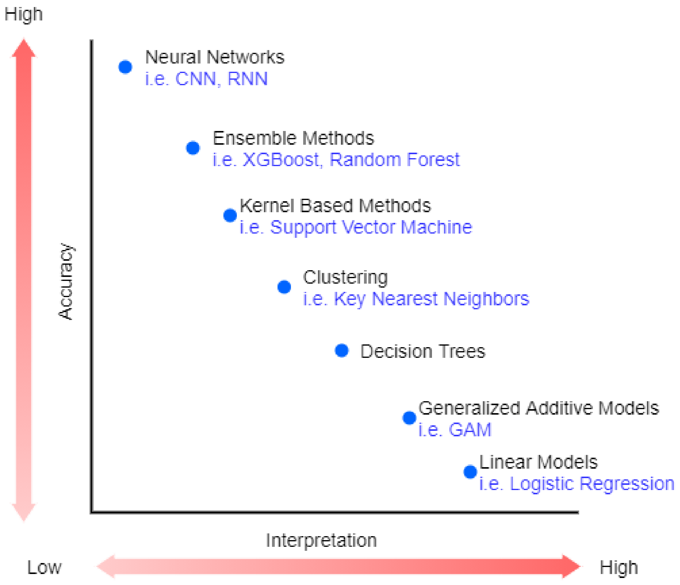
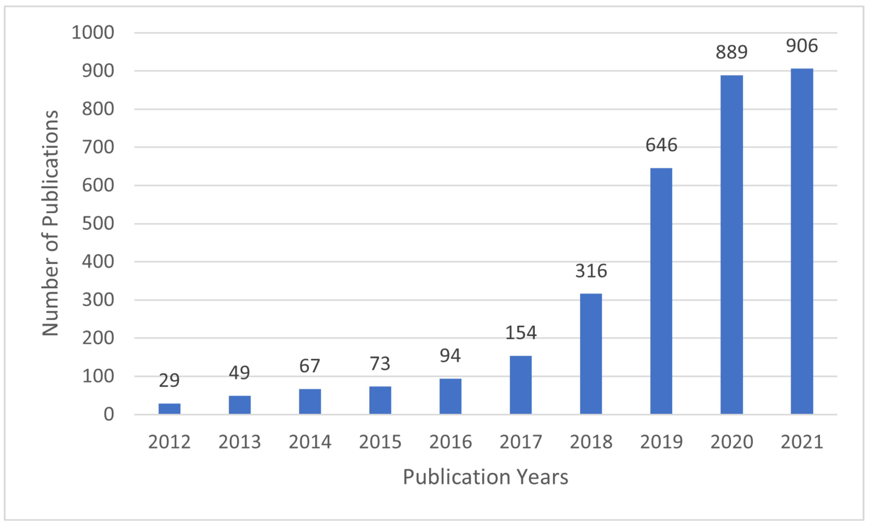
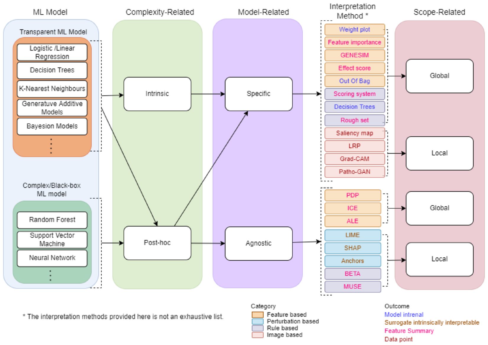
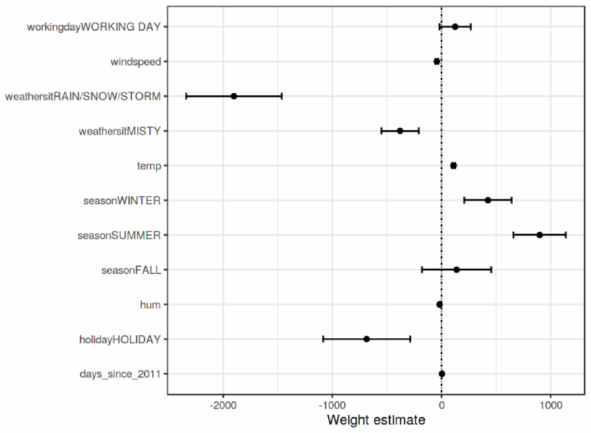
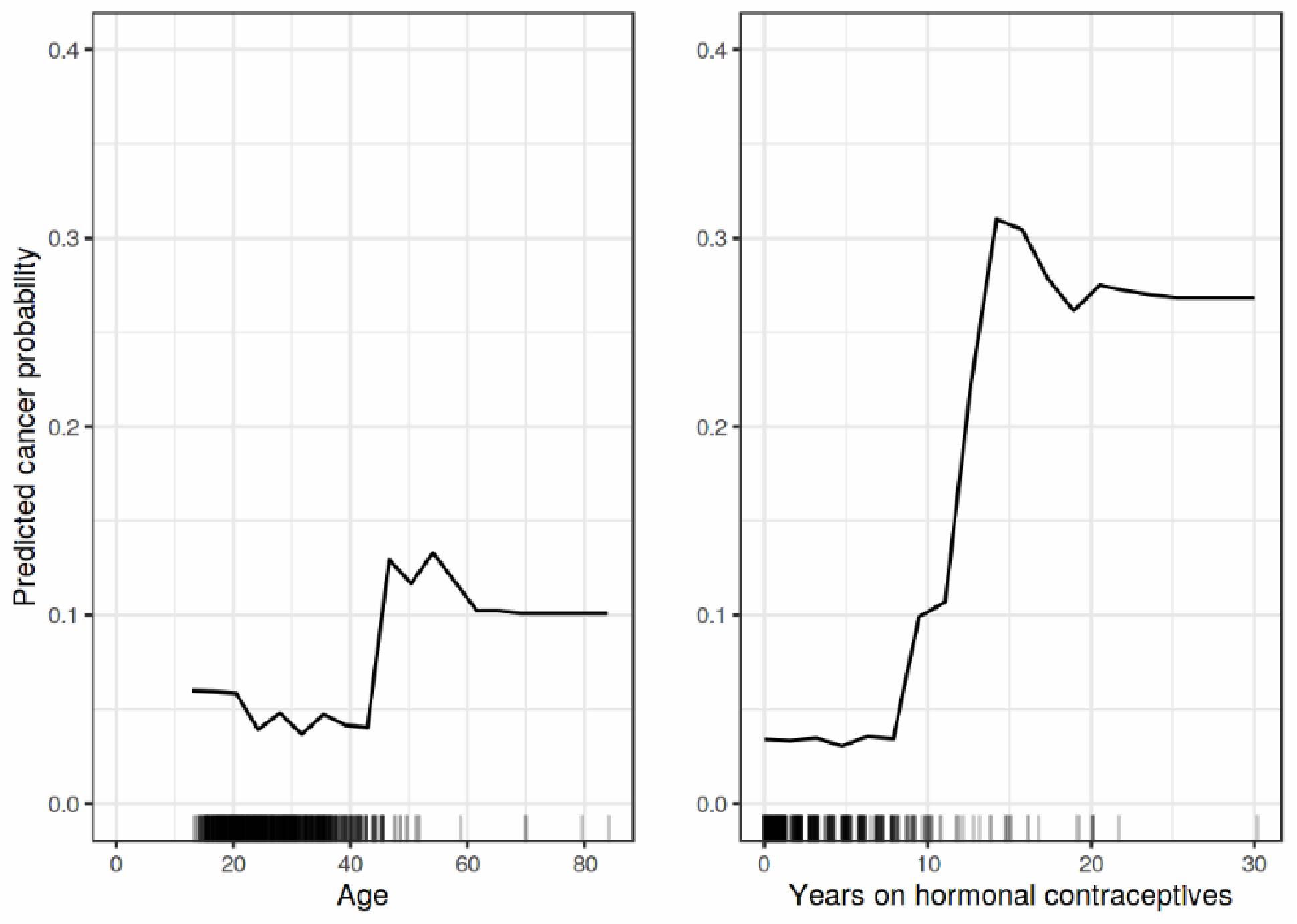
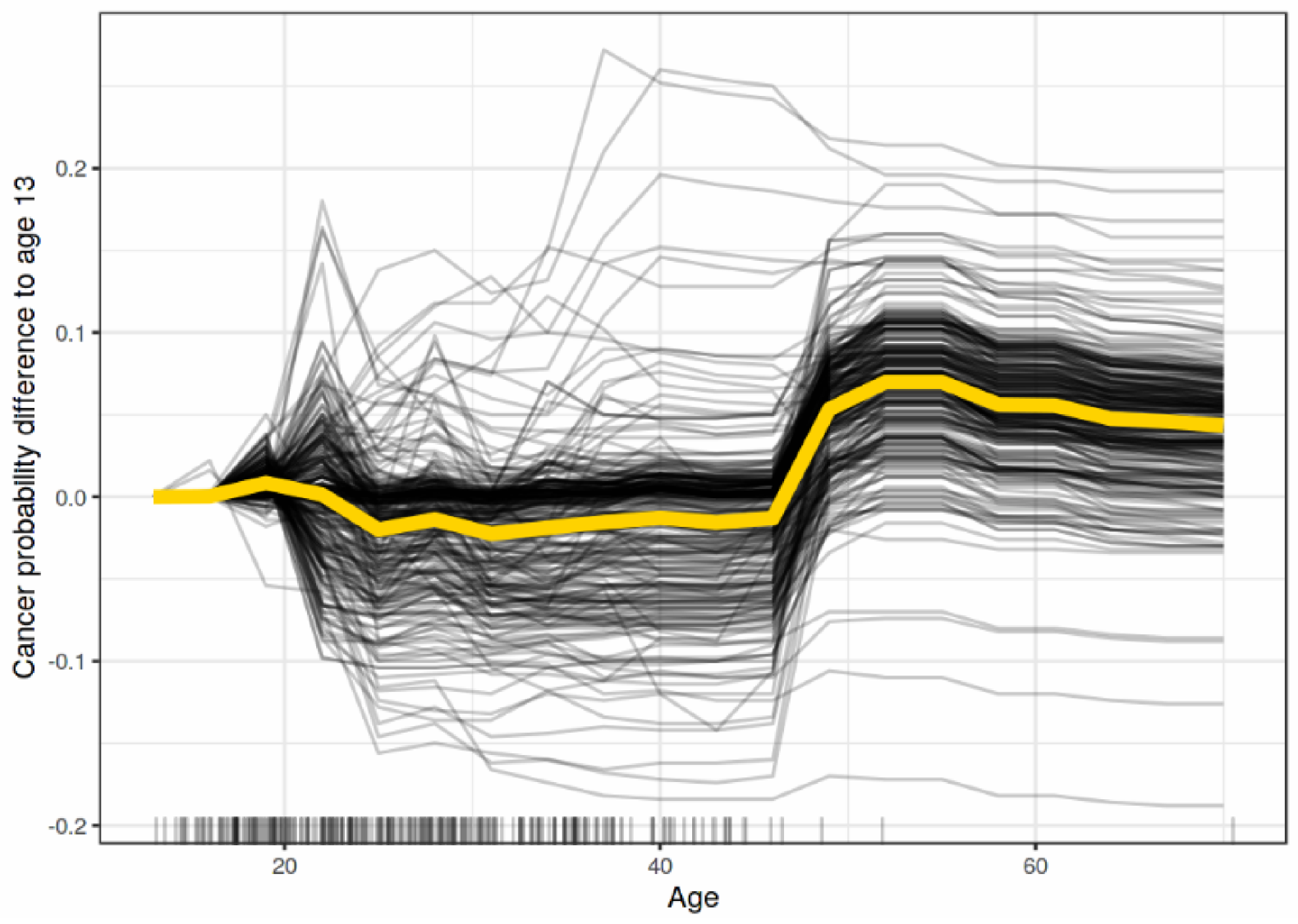
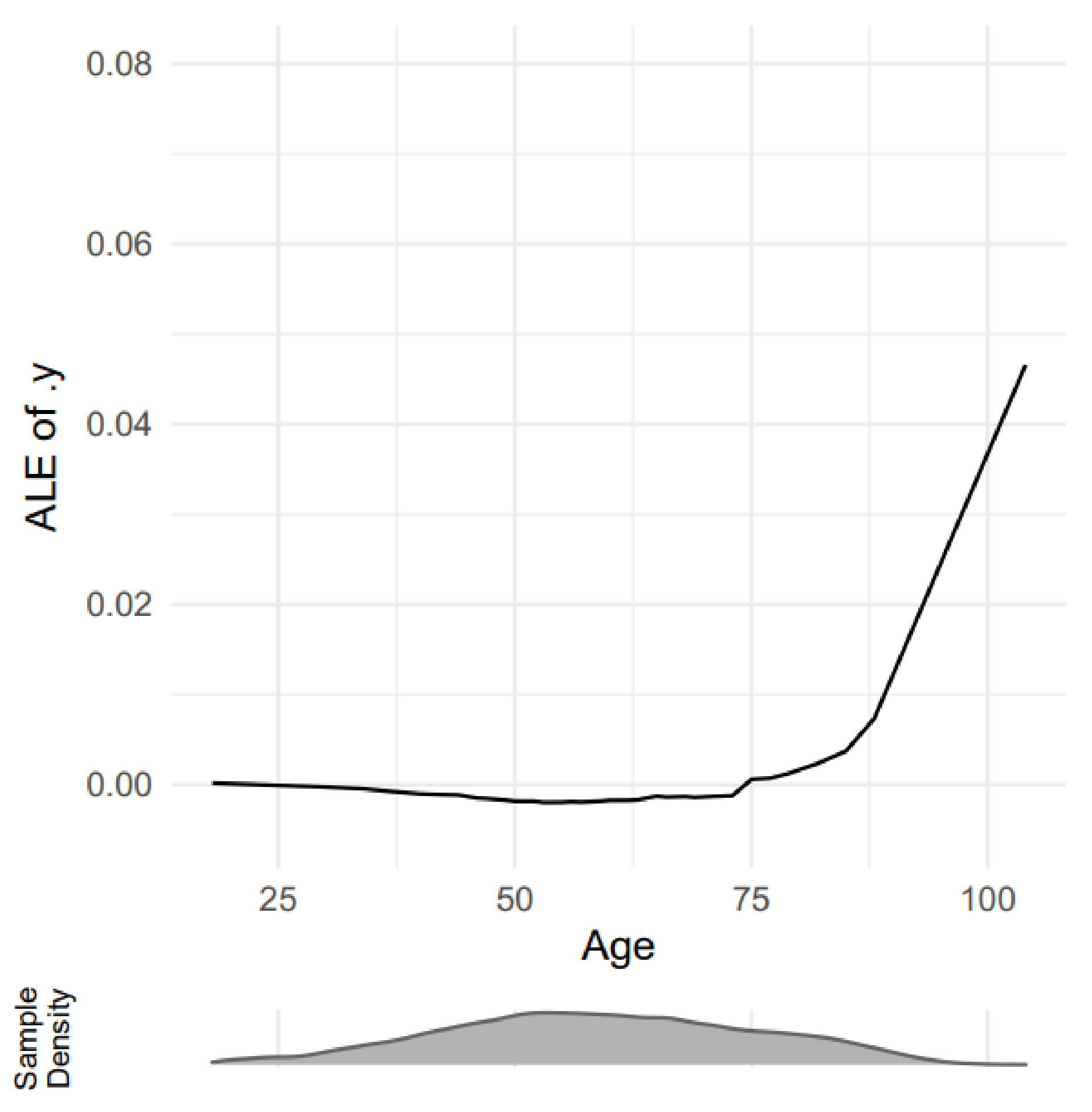
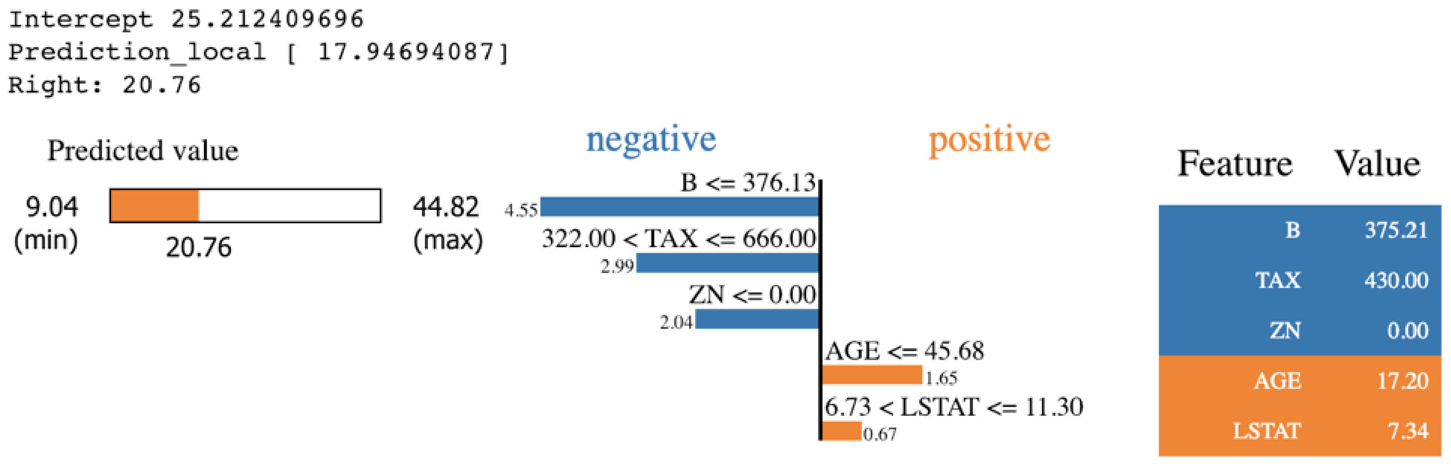
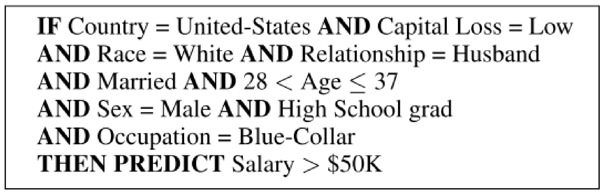
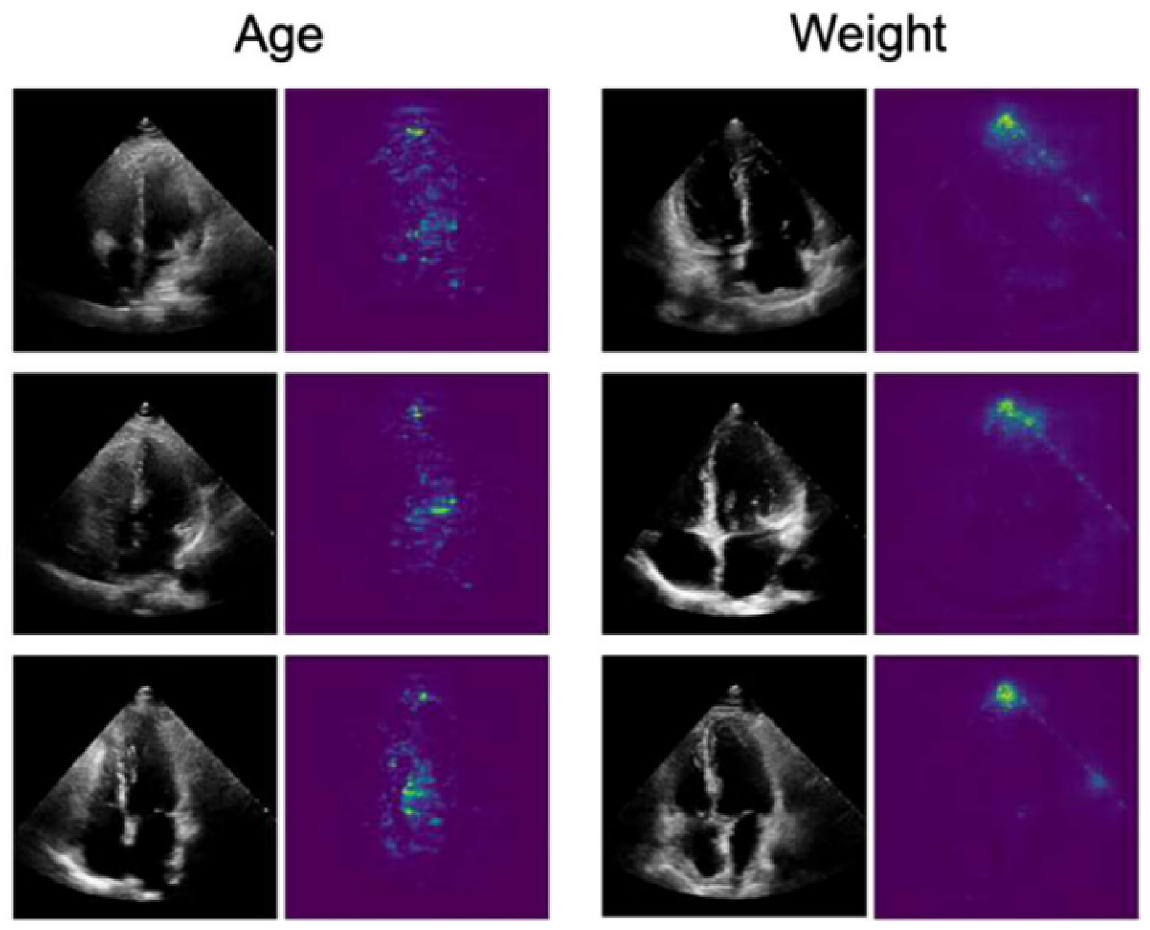
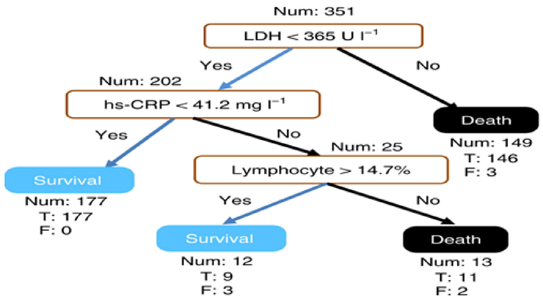
Table 1.
The pros and cons of model-related taxonomy.
| Model Type | Pros | Cons |
|---|---|---|
| Model-specific | Most method explanations are intuitive. Very fast. Highly translucent. Interpretations are more accurate. | Limited to a specific model. High switching cost. Feature selection is required to reduce dimensionality and enhance the explanation. |
| Model-agnostic | Easy to switch to another model. Low switching cost. No restrictions on the ML model. Not limited to a specific model. | Cannot access model internals. Interpretations are less accurate. |
Table 2.
Different IML methods, their category, and outcome presentation.
| Category | Approach | Complexity-Related | Model-Related | Scope-Related | Outcome | |||
|---|---|---|---|---|---|---|---|---|
| Intrinsic | Post-Hoc | Specific | Agnostic | Local | Global | |||
| Feature Based | Weight plot | √ | √ | √ | MI | |||
| Feature selection | √ | √ | √ | FS | ||||
| PDP | √ | √ | √ | FS | ||||
| ICE | √ | √ | √ | FS | ||||
| ALE | √ | √ | √ | FS | ||||
| GENESIM | √ | √ | √ | FS | ||||
| Effect score | √ | √ | √ | FS | ||||
| Out Of Bag | √ | √ | √ | FS | ||||
| Perturbation Based | LIME | √ | √ | √ | SI | |||
| SHAP | √ | √ | √ | FS | ||||
| Anchors | √ | √ | √ | SI | ||||
| Rule Based | Scoring system | √ | √ | √ | FS | |||
| Rough set | √ | √ | √ | FS | ||||
| BETA | √ | √ | √ | FS | ||||
| MUSE | √ | √ | √ | FS | ||||
| Decision Trees | √ | √ | √ | FS | ||||
| Image Based | Saliency map | √ | √ | √ | FS | |||
| LRP | √ | √ | √ | FS | ||||
| Grad-CAM | √ | √ | √ | FS | ||||
MI: Model internal; FS: Feature Summary; SI: Surrogate intrinsically interpretable.
Table 3.
Applications of IML in Healthcare.
| Disease | Reference | ML Algorithm | IML Method | Performance |
|---|---|---|---|---|
| Cardiovascular | [47], 2016 | Decision Trees | GENESIM | AC = 0.79 |
| [60], 2018 | Ensemble Predictor | Out-of-bag | AUC = 0.87 | |
| [61], 2020 | CNN | Saliency map | AUC = 0.89 | |
| [62], 2020 | XGBoost | SHAP | AC = 0.83 | |
| [63], 2020 | XGBoost | Tree SHAP | AUC = 0.71 | |
| [65], 2020 | XGBoost | Anchors, LIME, SHAP | AC = 0.98 | |
| [67], 2020 | XGBoost | OptiLIME | N/A | |
| [45], 2021 | SLSE | ALE | AUC = 0.87 | |
| [64], 2021 | 1D CNN | SHAP | AUC = 0.97 | |
| [46], 2021 | LR, RF, XGBoost | Effect score | AUC = 0.91 | |
| [59], 2021 | Patho-GAN | Patho-GAN | MSE = 0.01 | |
| [68], 2021 | XGboost | SHAP | AC = 0.95 | |
| [66], 2021 | RF | PDP | AUC = 0.90 | |
| Cancer | [53], 2013 | SLIM | Scoring System | AC = 0.97 |
| [69], 2019 | CNN | ALIME | AC = 0.95 | |
| [70], 2021 | XGBoos | Anchors, LIME, SHAP | AC = 0.78 | |
| Influenza and Infection | [71], 2020 | XGBoost | SHAP | AUC = 0.84 |
| [72], 2021 | DT, RF, ANN | ICE, PDP,ALE | F1 = 0.80 | |
| COVID-19 | [37], 2020 | XGBoost | Feature Importance | AC = 0.90 |
| [73], 2020 | DNN | Grad-CAM,LRP | F1 = 0.95 | |
| Depression | [54], 2017 | CNN | MUSE, BETA | AC= 0.98 |
| Autism | [74], 2021 | Rough set | Rule-based | AC = 0.90 |
Publisher’s Note: MDPI stays neutral with regard to jurisdictional claims in published maps and institutional affiliations. |
© 2021 by the authors. Licensee MDPI, Basel, Switzerland. This article is an open access article distributed under the terms and conditions of the Creative Commons Attribution (CC BY) license (https://creativecommons.org/licenses/by/4.0/).
Share and Cite
MDPI and ACS Style
Abdullah, T.A.A.; Zahid, M.S.M.; Ali, W. A Review of Interpretable ML in Healthcare: Taxonomy, Applications, Challenges, and Future Directions. Symmetry 2021, 13, 2439. https://0-doi-org.brum.beds.ac.uk/10.3390/sym13122439
AMA Style
Abdullah TAA, Zahid MSM, Ali W. A Review of Interpretable ML in Healthcare: Taxonomy, Applications, Challenges, and Future Directions. Symmetry. 2021; 13(12):2439. https://0-doi-org.brum.beds.ac.uk/10.3390/sym13122439
Chicago/Turabian StyleAbdullah, Talal A. A., Mohd Soperi Mohd Zahid, and Waleed Ali. 2021. "A Review of Interpretable ML in Healthcare: Taxonomy, Applications, Challenges, and Future Directions" Symmetry 13, no. 12: 2439. https://0-doi-org.brum.beds.ac.uk/10.3390/sym13122439
Note that from the first issue of 2016, this journal uses article numbers instead of page numbers. See further details here.