
A Hierarchical Universal Algorithm for Geometric Objects’ Reflection Symmetry Detection

 , , , , , and
Abstract
:1. Introduction
- The algorithm detects the global reflection symmetry;
- It accepts a point cloud obtained by sampling the input geometric object’s surface;
- It works for 2D as well for 3D geometric objects with just a few small adaptations;
- It accepts objects without holes as well as those with holes, which may even be nested;
- Geometric objects may be open or closed;
- The algorithm is designed for acceleration by three techniques—by a two-level uniform subdivision; by varying the granularity of the testing symmetry axes/planes; and by parallelisation.
2. Related Works
2.1. Global Reflection Symmetry
2.2. Local Reflection Symmetry
2.3. Global Reflection and Rotational Symmetry
2.4. Different Categories of Local Symmetry
2.5. Machine Learning in Symmetry Detection
3. Materials and Methods
- 1.
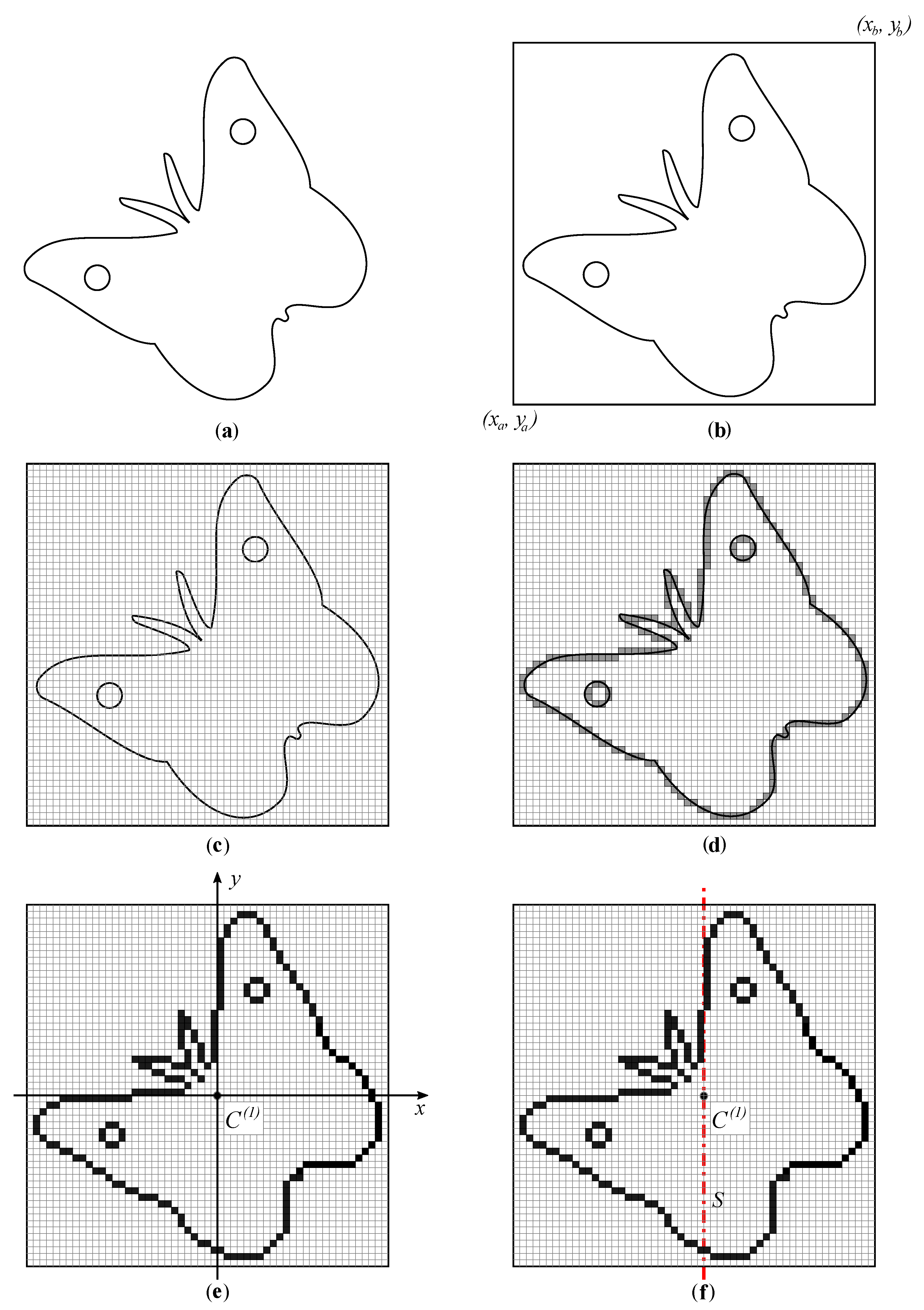
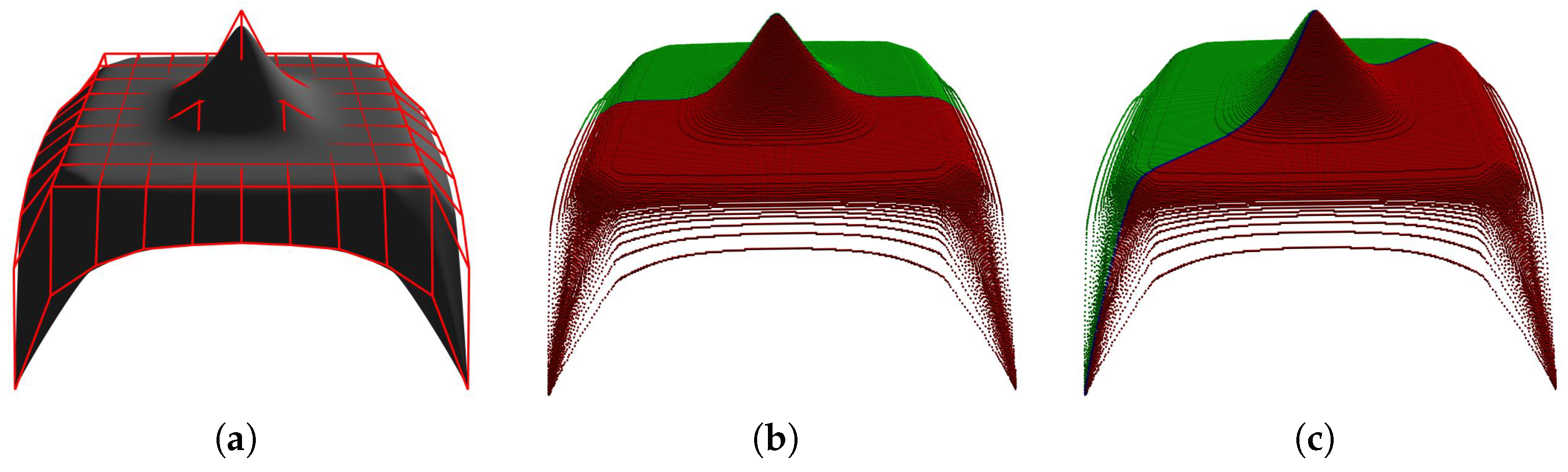
- The information about the object’s boundary, labelled hereafter, is obtained first. The object may contain holes; two are presented in the particular example in Figure 1a. Initially, the geometry is expressed in the Cartesian coordinate system adopted from the input dataset.
- 2.
- An axis-aligned bounding rectangle (a bounding box in 3D) is subsequently determined. It is specified by the bottom left and the top right points , where in 2D (see Figure 1b).
- 3.
- The axis-aligned bounding rectangle/box is divided into equally sized cells u forming a uniform grid U, , as shown in Figure 1c. The number of cells in each coordinate direction is determined by heuristic (1), where .m in (1) represents the linear size of a cell in any coordinate direction.
- 4.
- The tolerance is then determined by which the allowed deviation from the ideal symmetry of is enabled. The tolerance should at least compensate for the effect of the uniform grid usage. is set by default; however, it can be changed by the user.
- 5.
- The ’s boundary is uniformly sampled by the horizontal and vertical sampling step of . The obtained sampled points of are inserted into U and the set of boundary cells of is determined. A cell u, , belongs to the object () if u contains at least one point of . Two cells are neighbours if they share a common edge in 2D or a common side in 3D. We may now formally define . The cells of are plotted in grey in Figure 1d.
- 6.
- 7.
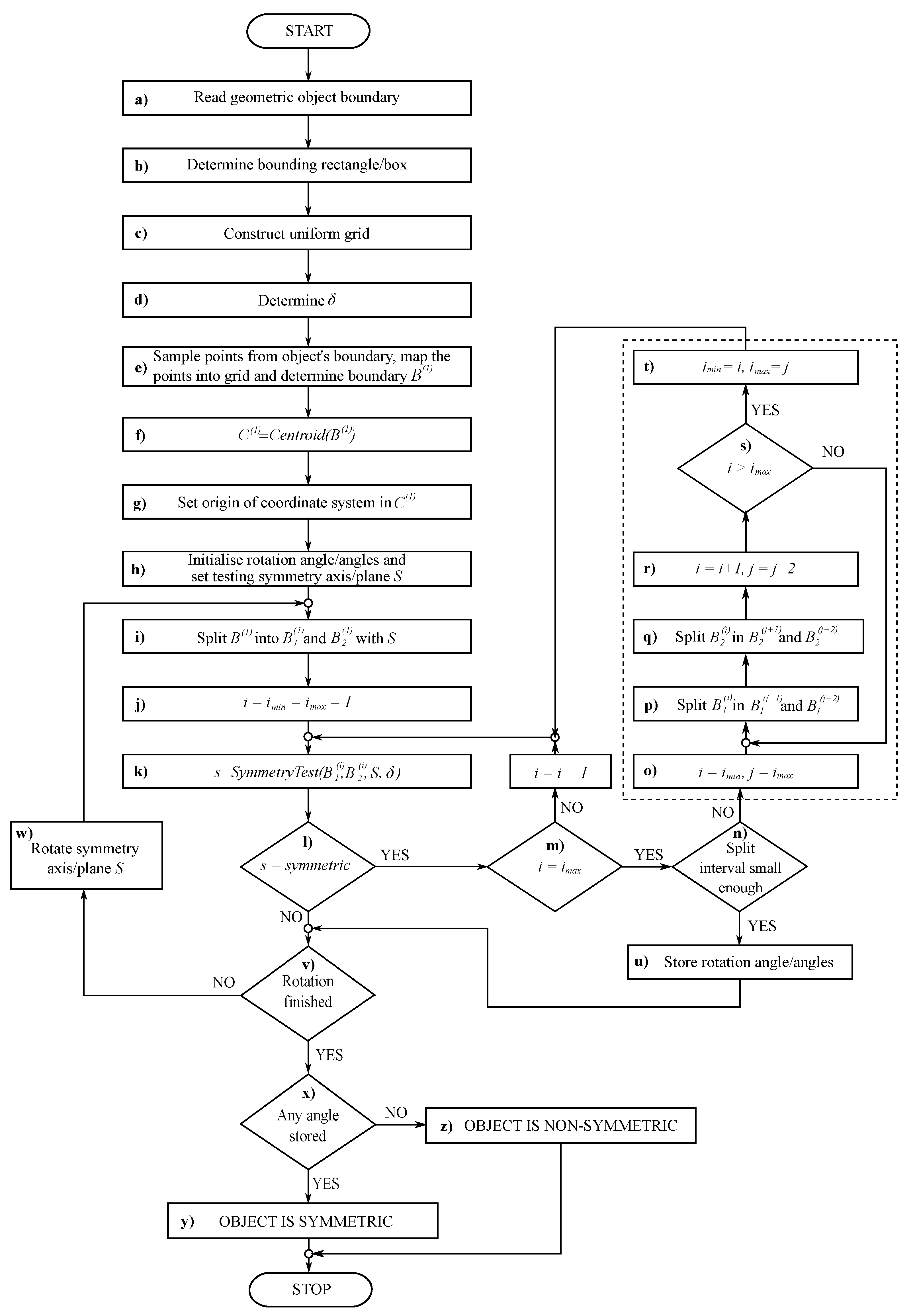
- A testing axis of symmetry S (a testing plane in 3D) is then placed in the origin (red dot-dashed line in Figure 1f). In general, S can be arbitrarily sloped at the beginning. However, it is desired that S is initially aligned with one of the coordinate axes in 2D or with one of the coordinate planes in 3D. In Figure 1f, S coincides with the y axis.
- 8.
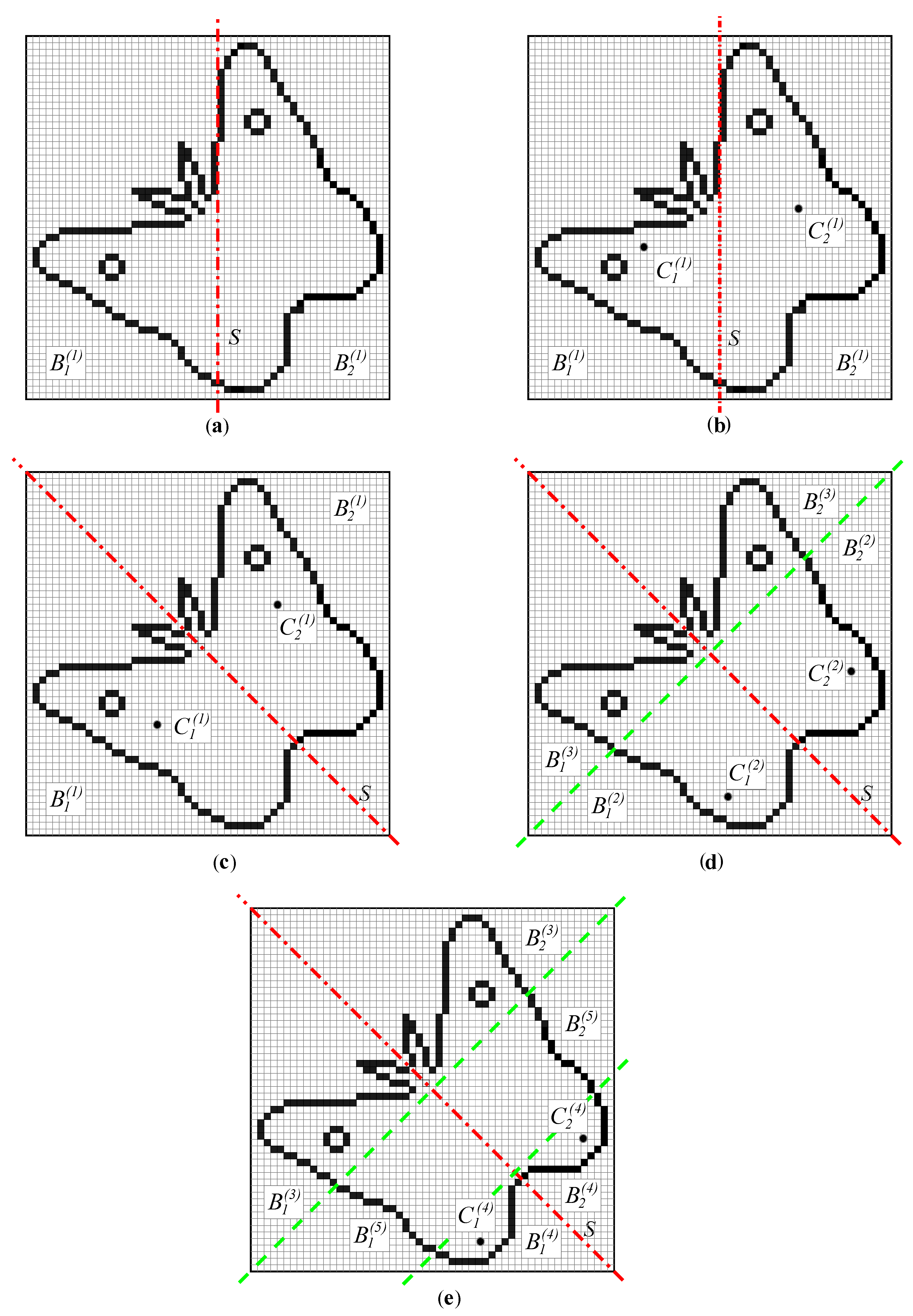
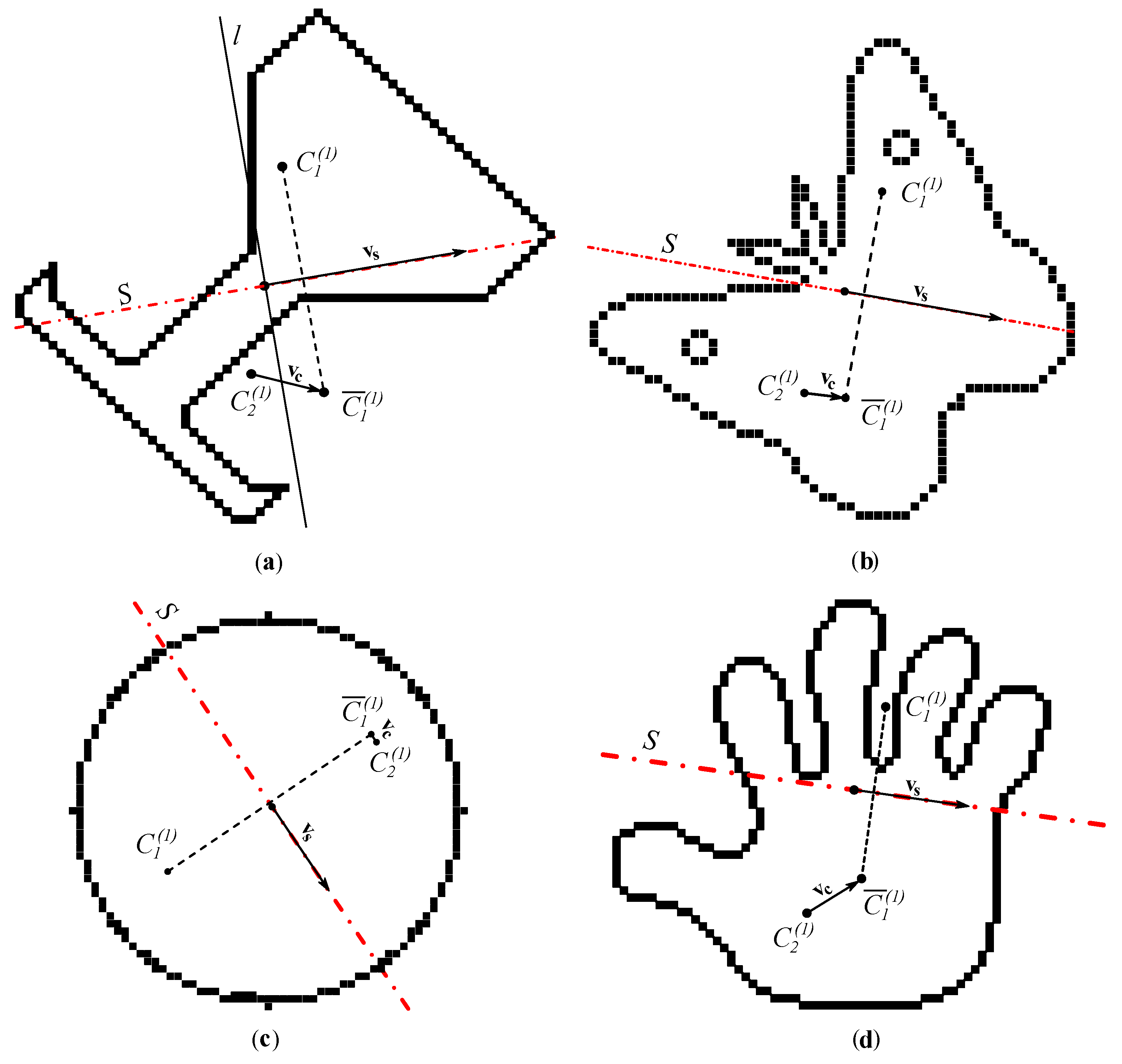
- S divides into two subsets an , as seen in Figure 2a.
- 9.
- A function SymmetryTest is then used. This function calculates two auxiliary centroids for and for (Figure 2b shows an initial situation when ). In addition, a common centroid for and is calculated according to (3). and represent the cardinalities of the corresponding sets. This part of the algorithm is hierarchically repeated as later described with the flowchart (Figure 3) and an example (Figure 4). In the first repetition, equals calculated in step 6.The function SymmetryTest returns either symmetric or non-symmetric. If the claims given in (4) are valid, the returned value is symmetric. The first claim states that the two centroids are equidistant from the testing axis/plane S. The second claim says that the line through the centroids is perpendicular to S, and the third claim checks whether the subsets and are balanced with respect to S, so that the common centroid is on S. All three conditions are necessary because they are independent of each other. Function d, as used in (4), calculates a non-negative distance between two points, or between a point and S.
- 10.
- Sets and are further split by the line/plane perpendicular to S. With each split, i is incremented. The function SymmetryTest is repeatedly called for a split pair of subsets until the threshold for the division is reached (a suitable threshold is 2 m, for example) or the function returns non-symmetric. If symmetric is returned in all runs of the SymmetryTest, the object is considered symmetric in the actual orientation, and the rotation angle (two angles in 3D) of the symmetry axis/plane is stored.
- 11.
- S is rotated for a small angle (e.g., ) and the algorithm returns to step 9 if not all rotation positions have been checked yet. Otherwise, the algorithm verifies whether at least one angle was stored in the previous steps. The object is declared to be symmetric in this case, otherwise it is non-symmetric.
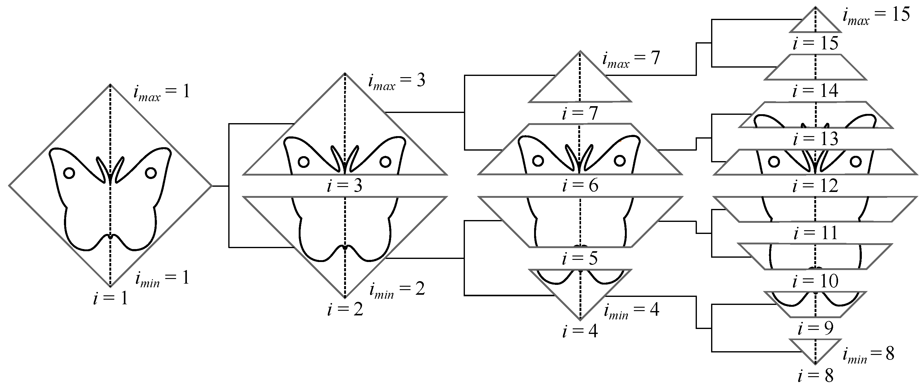
- Level 0 (root level). Block i sets both, and to 1 and initialises . After a single iteration, the loop termination condition in block m is true, and the hatched block is entered. Blocks p and q split the root node into and . The loop indicated by termination condition s is exited with , , and . Accordingly, block t sets and , making the next tree level ready for processing.
- Level 1. Nodes and are both successfully tested for symmetry before the loop termination condition in block m becomes true. Blocks p and q within the loop in the hatched block split into the pair of nodes (, ) and into (, ). The loop is exited with , , and . Accordingly, block t sets and .
- Level 2. Nodes – are all successfully tested for symmetry before the loop termination condition in block m becomes true. Blocks p and q within the loop in the hatched block split into (, ), into (, ), into (, ), and into (, ). The loop is exited with , , and . Accordingly, block t sets and .
- Level 3. Nodes – are all successfully tested for symmetry before the loop termination condition in block m is true. This depends on the predefined splitting threshold tested in the loop termination condition n, whether the algorithm proceeds to the hatched block to split these nodes further or it terminates the symmetry test for the considered rotated position of S.
- Mode A:
- All symmetry axes/planes in are determined within the granularity .
- Mode B:
- The first found symmetry axis/plane is returned.
- Mode C:
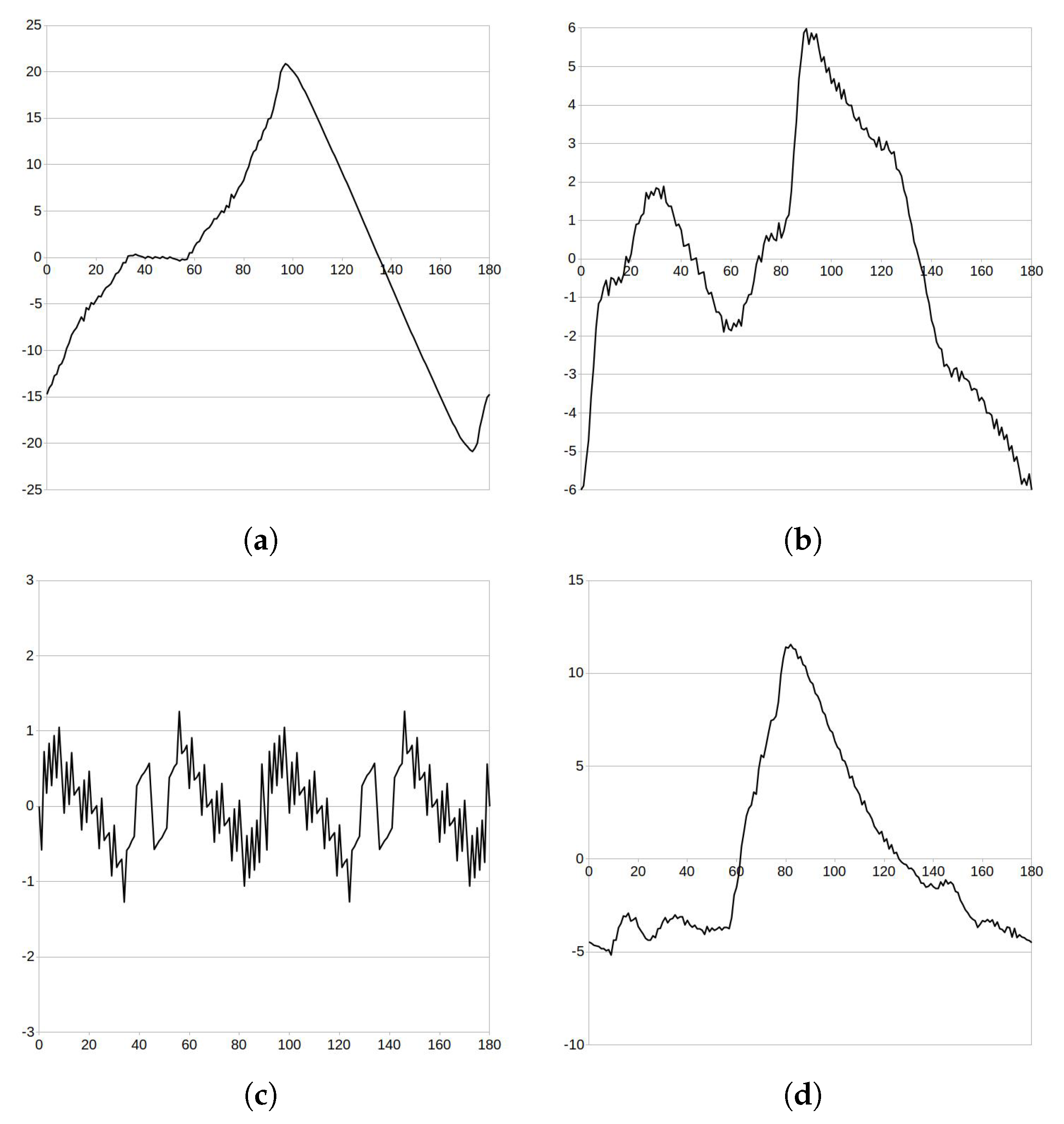
- The algorithm determines the closest axis/plane to the ideal symmetry axis/plane for non-symmetric . It searches for S where the Euclidean distance between and the mirrored image of across S is the smallest.
3.1. Algorithm Acceleration
- 1.
- Computes the centroids of , , and in time .
- 2.
- Evaluates inequality (4) in time .
- 3.
- Splits and perpendicularly to S into two pairs of subsets in time .
- l be the number of hierarchical levels of execution of the algorithm.
- indicate the maximum value of l.
- and , , be the start and end index i of , , and at level h.
- stand for the granularity of the slope increment of S.
- D be the dimension .
- Diagonal be the length of the diagonal of the bounding box int 3D or a bounding rectangle in 2D.
3.1.1. Dual-Resolution Grid
- It starts with , splits it into and , and runs SymmetryTest .
- If the SymmetryTest returns symmetric, the algorithm switches to U and gradually considers the split sub-problems until SymmetryTest = non-symmetric or the subdivision threshold is reached.
3.1.2. Variable Granularity of the Testing Axis/Plane
- Does observing prevent false positives?
- Does observing prevent false negatives?
3.1.3. Parallelisation
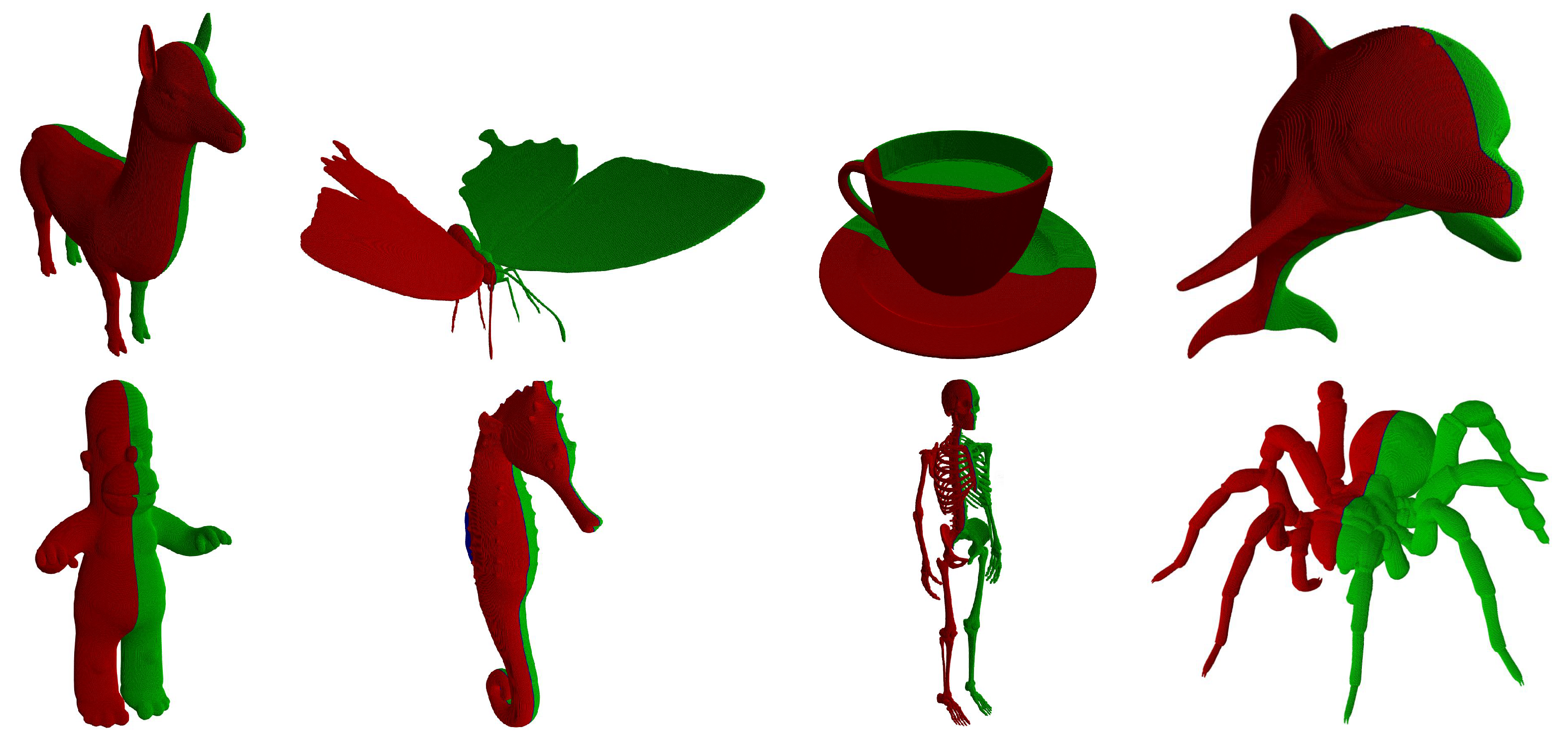
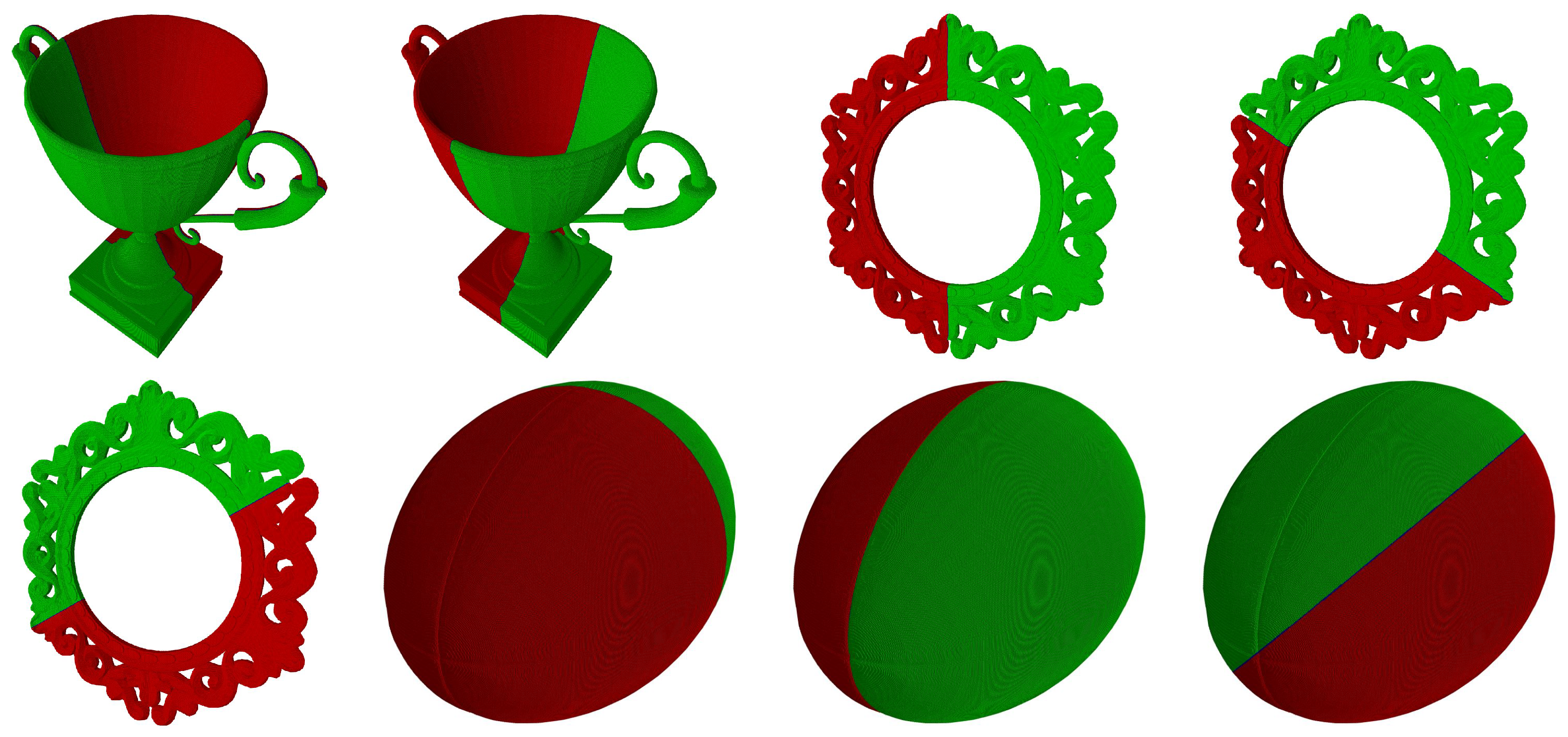
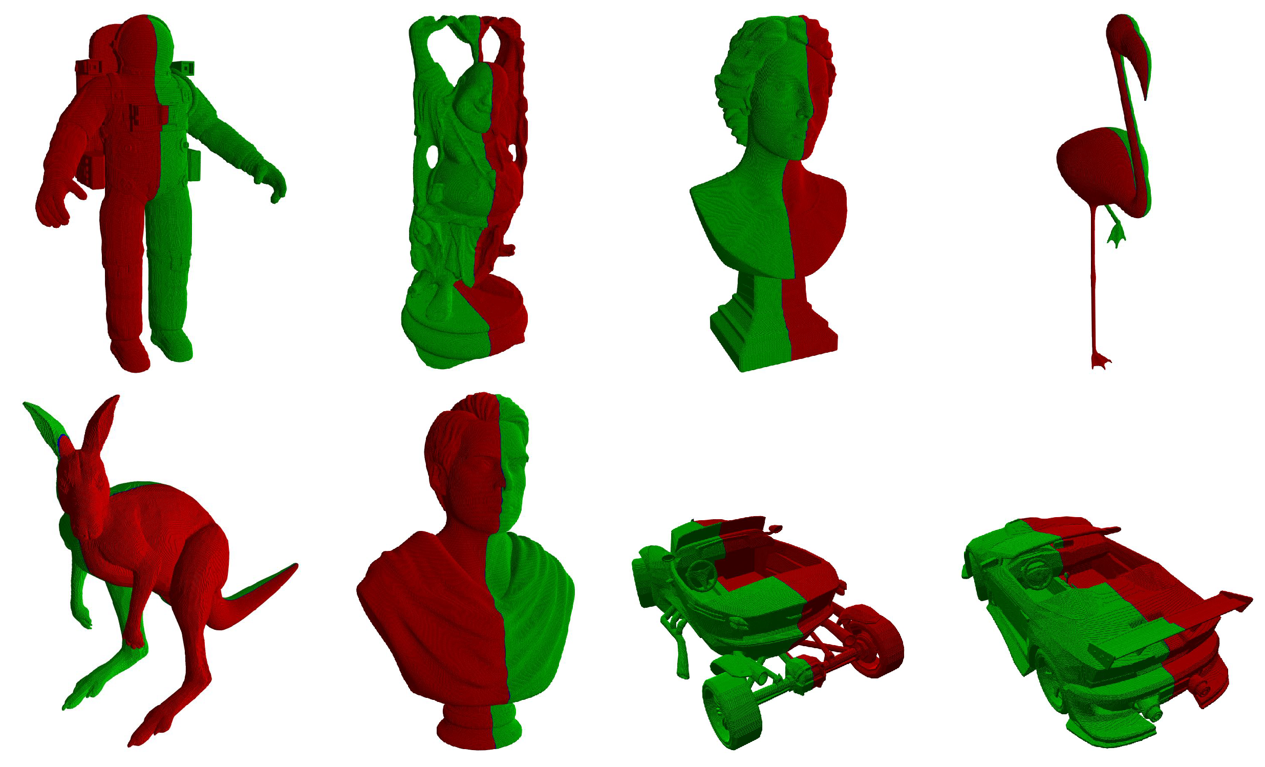
4. Results
5. Discussion
Author Contributions
Funding
Institutional Review Board Statement
Informed Consent Statement
Data Availability Statement
Conflicts of Interest
References
- McManus, I.C. Symmetry and Asymmetry in Aesthetics and the Arts. Eur. Rev. 2005, 13, 157–180. [Google Scholar] [CrossRef]
- Mehaffy, M.W. The Impacts of Symmetry in Architecture and Urbanism: Toward a New Research Agenda. Buildings 2020, 10, 249. [Google Scholar] [CrossRef]
- Evans, C.S.; Wenderoth, P.; Cheng, K. Detection of Bilateral Symmetry in Complex Biological Images. Perception 2000, 29, 31–42. [Google Scholar] [CrossRef]
- Qui, W.; Yuan, J.; Ukwatta, E.; Sun, Y.; Rajchl, M.; Fenster, A. Prostate Segmentation: An Efficient Convex Optimization Approach With Axial Symmetry Using 3-D TRUS and MR Images. IEEE Trans. Med. Imaging 2014, 33, 947–960. [Google Scholar]
- Jäntschi, L.; Bolboacã, S.D. Symmetry in Applied Mathematics; MDPI: Basel, Switzerland, 2020. [Google Scholar]
- Glowacz, A.; Królczyk, G.; Antonino-Daviu, J.A. Symmetry in Mechanical Engineering; MDPI: Basel, Switzerland, 2020. [Google Scholar]
- Modrea, A.; Munteanu, V.M.; Pruncu, I. Using the Symmetries in the Civil Engineering. An overview. Procedia Manuf. 2020, 46, 906–913. [Google Scholar] [CrossRef]
- Montoya, F.G.; Navarro, R.B. Symmetry in Engineering Sciences; MDPI: Basel, Switzerland, 2019. [Google Scholar]
- Weyl, H. Symmetry; Princenton University Press: New York, NY, USA, 1952. [Google Scholar]
- Miller, W. Symmetry Groups and Their Applications; Academic Press: London, UK, 1972. [Google Scholar]
- Liu, X.; Hel-Or, H.; Kaplan, C.S.; van Gool, L. Computational Symmetry in Computer Vision and Computer Graphics. Found. Trends Comput. Graph. Vis. 2009, 5, 1–195. [Google Scholar] [CrossRef]
- Martin, G.E. Transformation Geometry; Springer: New York, NY, USA, 1982. [Google Scholar]
- Barker, W.H.; Howe, R. Continuous Symmetry: From Euclid to Klein; American Mathematical Society: Providence, RI, USA, 2007. [Google Scholar]
- Leyton, M. Symmetry, Causality, Mind; MIT Press: Cambridge, MA, USA, 1992. [Google Scholar]
- Ponce, J. On Characterizing Ribbons and Finding Skewed Symmetries. Comput. Vis. Graph. Image Process. 1990, 52, 328–340. [Google Scholar] [CrossRef]
- Conners, R.W.; Ng, C.T. Developing a Quantitative Model of Human Preattentive Vision. IEEE Trans. Syst. Man Cybernet. 1989, 19, 1384–1407. [Google Scholar] [CrossRef]
- Tyler, C.W. Human Symmetry Perception and its Computational Analysis; Lawrence Erlbaum Associates: Mahwah, NJ, USA, 2002. [Google Scholar]
- Xiao, Z.; Wu, J. Analysis on Image Symmetry Detection Algorithms. In Proceedings of the Fourth International Conference on Fuzzy Systems and Knowledge Discovery (FSKD 2007), Haikou, China, 24–27 August 2007; pp. 745–750. [Google Scholar]
- Mitra, N.J.; Pauly, M.; Wand, M.; Ceylan, D. Symmetry in 3D geometry: Extraction and applications. Comput. Graph. Forum 2013, 32, 1–23. [Google Scholar] [CrossRef]
- Bartalucci, C.; Furferi, R.; Governi, L.; Volpe, Y. A Survey of Methods for Symmetry Detection on 3D High Point Density Models in Biomedicine. Symmetry 2018, 10, 263. [Google Scholar] [CrossRef] [Green Version]
- Elawady, M.; Ducottet, C.; Alata, O.; Barat, C.; Colantoni, P. Wavelet-Based Reflection Symmetry Detection via Textural and Color Histograms: Algorithm and Results. In Proceedings of the 2017 IEEE International Conference on Computer Vision Workshops (ICCVW), Venice, Italy, 22–29 October 2017; pp. 1734–1738. [Google Scholar]
- Chen, H.; Wang, L.; Zhang, Y.; Wang, C. Dominant Symmetry Plane Detection for Point-Based 3D Models. Adv. Multimed. 2020, 2020, 8861367. [Google Scholar]
- Schiebener, D.; Schmidt, A.; Vahrenkamp, N.; Asfour, T. Heuristic 3D Object Shape Completion Based on Symmetry and Scene Context. In Proceedings of the IEEE/RSJ International Conference on Intelligent Robots and Systems (IROS), Daejeon, Korea, 9–14 October 2016; pp. 74–81. [Google Scholar]
- Combés, B.; Hennessy, R.; Waddington, J.; Roberts, N.; Prima, S. Automatic Symmetry Plane Estimation of Bilateral Objects in Point Clouds. In Proceedings of the IEEE Conference on Computer Vision and Pattern Recognition, Anchorage, AK, USA, 23–28 August 2008; pp. 1–8. [Google Scholar]
- Ecins, A.; Fermüller, C.; Aloimonos, Y. Detecting Reflectional Symmetries in 3D Data Through Symmetrical Fitting. In Proceedings of the IEEE International Conference on Computer Vision Workshops (ICCVW), Venice, Italy, 22–29 October 2017; pp. 1779–1783. [Google Scholar]
- Nagar, R.; Raman, S. Detecting Approximate Reflection Symmetry in a Point Set Using Optimization on Manifold. IEEE Trans. Signal Process. 2019, 67, 1582–1595. [Google Scholar] [CrossRef] [Green Version]
- Hruda, L.; Kolingerová, I.; Váša, L. Robust, Fast, Flexible Symmetry Plane Detection Based on Differentiable Symmetry Measure. Vis. Comput. 2022, 38, 555–571. [Google Scholar] [CrossRef]
- Li, B.; Johan, H.; Ye, Y.; Lu, Y. Efficient 3D Reflection Symmetry Detection: A View-based Approach. Graph. Models 2016, 83, 2–14. [Google Scholar] [CrossRef]
- Sipiran, I.; Gregor, R.; Schreck, T. Approximate Symmetry Detection in Partial 3D Meshes. Comput. Graph. Forum 2014, 33, 131–140. [Google Scholar] [CrossRef] [Green Version]
- Kakarala, R.; Kaliamoorthi, P.; Premachandran, V. Three-Dimensional Bilateral Symmetry Plane Estimation in the Phase Domain. In Proceedings of the IEEE Conference on Computer Vision and Pattern Recognition, Portland, OR, USA, 23–28 June 2013; pp. 249–256. [Google Scholar]
- Podolak, J.; Shilane, P.; Golovinsky, A.; Rusinkiewiczm, S.; Funkhouser, T. A Planar-Reflective Symmetry Transform for 3D Shapes. ACM Trans. Graph. 2006, 25, 549–559. [Google Scholar] [CrossRef]
- Cicconet, M.; Hildebrand, D.G.C.; Elliott, H. Finding Mirror Symmetry via Registration and Optimal Symmetric Pairwise Assignment of Curves: Algorithm and Results. In Proceedings of the IEEE International Conference on Computer Vision Workshops (ICCVW), Venice, Italy, 22–29 October 2017; pp. 1759–1763. [Google Scholar]
- Simari, P.D.; Kalogerakis, E.; Singh, K. Folding meshes: Hierarchical Mesh Segmentation Based on Planar Symmetry. In Proceedings of the Fourth Eurographics Symposium on Geometry Processing, Cagliary, Italy, 26–28 June 2006; pp. 111–119. [Google Scholar]
- Cailliere, D.; Denis, F.; Pele, D.; Baskurt, A. 3D Mirror Symmetry Detection Using Hough Transform. In Proceedings of the 5th IEEE International Conference on Image Processing, San Diego, CA, USA, 12–15 October 2008; pp. 1772–1775. [Google Scholar]
- Speciale, P.; Oswald, M.R.; Cohen, A.; Pollefeys, M. A Symmetry Prior for Convex Variational 3D Reconstruction. In Computer Vision—ECCV 2016; Leibe, B., Matas, J., Sebe, N., Welling, M., Eds.; Lecture Notes in Computer Science 9912; Springer: Cham, Germany, 2016; pp. 313–328. [Google Scholar]
- Liu, Y.-K.; Žalik, B.; Wang, P.-J.; Podgorelec, D. Directional Difference Chain Codes with Quasi-Lossless Compression and Run-Length Encoding. Signal Process. Image Commun. 2012, 27, 973–984. [Google Scholar] [CrossRef]
- Bribiesca, E. A Measure of Tortuosity Based on Chain Coding. Pattern Recognit. 2013, 46, 716–724. [Google Scholar] [CrossRef]
- Alvarado-Gonzalez, M.; Aguilar, W.; Garduño, E.; Velarde, C.; Bribiesca, E.; Medina-Bañuelos, V. Mirror Symmetry Detection in Curves Represented by Means of the Slope Chain Code. Pattern Recognit. 2019, 87, 67–79. [Google Scholar] [CrossRef]
- Aguilar, W.; Alvarado-Gonzalez, M.; Garduño, E.; Velarde, C.; Bribiesca, E. Detection of Rotational Symmetry in Curves Represented by the Slope Chain Code. Pattern Recognit. 2020, 107, 107421. [Google Scholar] [CrossRef]
- Sun, C.; Sherrah, J. 3D Symmetry Detection Using the Extended Gaussian Image. IEEE Trans. Pattern Anal. 1997, 19, 164–168. [Google Scholar]
- Korman, S.; Litman, R.; Avidan, S.; Bronstein, A. Probably Approximately Symmetric: Fast Rigid Symmetry Detection with Global Guarantees. Comput. Graph. Forum 2015, 34, 2–13. [Google Scholar] [CrossRef] [Green Version]
- Mitra, N.J.; Guibas, L.J.; Pauly, M. Approximate Symmetry Detection for 3D Geometry. ACM Trans. Graph. 2006, 25, 560–668. [Google Scholar] [CrossRef]
- Ji, P.; Liu, X. A Fast and Efficient 3D Reflection Symmetry Detector Based on Neural Networks. Multimed. Tools Appl. 2019, 78, 35471–35492. [Google Scholar] [CrossRef]
- Wu, Z.; Jiang, H.; He, S. Symmetry Detection of Occluded Point Cloud Using Deep Learning. Procedia Comput. Sci. 2021, 183, 32–39. [Google Scholar] [CrossRef]
- Gao, L.; Zhang, L.-X.; Meng, H.-Y.; Ren, Y.-H.; Lai, Y.-K.; Kobbelt, L. PRS-Net: Planar Reflective Symmetry Detection Net for 3D Models. IEEE Trans. Vis. Comput. Graph. 2021, 27, 3007–3018. [Google Scholar] [CrossRef]
- Tsogkas, S.; Kokkinos, I. Learning-based Symmetry Detection in Natural Images. In Computer Vision—ECCV 2012 Florence; Fitzgibbon, A., Lazebnik, S., Perona, P., Sato, Y., Schmid, C., Eds.; Lecture Notes in Computer Science 7578; Springer: Berlin/Heidelberg, Germany, 2012; pp. 41–54. [Google Scholar]
- Mattson, T.G.; He, Y.; Koniges, A.E. The OpenMP Commom Core, Making OpenMP Simple Again; MIT Press: Cambridge, MA, USA; London, UK, 2019. [Google Scholar]
- Generalized Symmetries and Equivalences of Geometric Data. Supplementary Material. Available online: https://gemma.feri.um.si/projects/international-projects/generalized-symmetries-and-equivalences-of-geometric-data-si/eng/software-eng/ (accessed on 11 April 2022).
- PLY Files an ASCII Polygon Format. Available online: https://people.sc.fsu.edu/~jburkardt/data/ply/ply.html (accessed on 24 February 2022).
- The Stanford 3D Scanning Repository. Available online: http://graphics.stanford.edu/data/3Dscanrep/ (accessed on 24 February 2022).
- MS Paint3D Library. Available online: https://free3d.com/3d-model (accessed on 24 February 2022).
- Guid, N.; Kolmanič, S.; Strnad, D. SURFMOD: Teaching tool for parametric curve and surface methods in CAGD based on comparison and analysis. IEEE Trans. Educ. 2006, 49, 292–301. [Google Scholar] [CrossRef]
- Moller, A.P. Swallows and Scorpionflies Find Symmetry is Beautiful. Science 1992, 257, 327–328. [Google Scholar]


| Object | Symmetric? | |
|---|---|---|
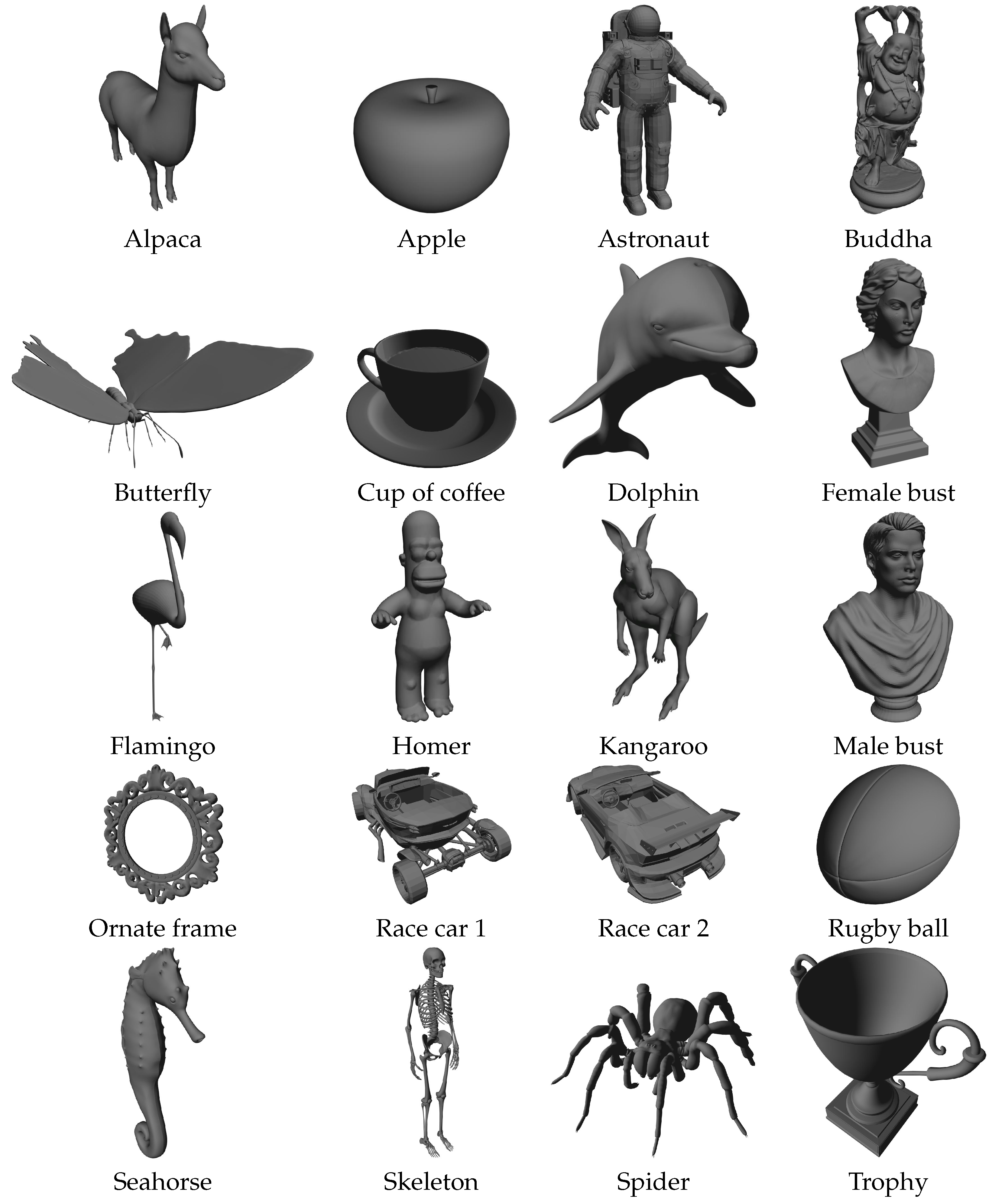
| Alpaca | 1,322,413 | ✓ |
| Apple | 1,898,806 | ✓✓ |
| Astronaut | 2,381,281 | × |
| Buddha | 1,815,195 | × |
| Butterfly | 1,602,828 | ✓ |
| Coffee cup | 3,717,007 | ✓ |
| Dolphin | 836,102 | ✓ |
| Female bust | 1,703,742 | × |
| Flamingo | 431,892 | × |
| Homer | 1,234,423 | ✓ |
| Kangaroo | 836,738 | × |
| Male bust | 2,035,006 | × |
| Ornate frame | 1,304,854 | ✓✓ |
| Race car 1 | 3,490,257 | × |
| Race car 2 | 2,908,840 | × |
| Rugby ball | 951,947 | ✓✓ |
| Seahorse | 709,877 | ✓ |
| Skeleton | 560,303 | ✓ |
| Spider | 1,374,073 | ✓ |
| Trophy | 3,369,891 | ✓✓ |
| Object | Single Thread | Multi-Threaded | |||
|---|---|---|---|---|---|
| Basic | Accelerated | Basic | Accelerated | Referenced | |
| Alpaca | 299.15 | 0.374 | 28.03 | 0.044 | 0.230 |
| Apple | 424.50 | 0.430 | 42.27 | 0.151 | 0.193 |
| Astronaut | 267.21 | 0.592 | 52.89 | 0.077 | 0.254 |
| Buddha | 407.90 | 0.564 | 40.24 | 0.133 | 0.431 |
| Butterfly | 353.86 | 0.360 | 36.19 | 0.046 | 0.167 |
| Coffee cup | 839.88 | 0.426 | 84.38 | 0.079 | 0.187 |
| Dolphin | 180.64 | 0.195 | 12.88 | 0.044 | 0.245 |
| Female bust | 376.64 | 0.345 | 37.51 | 0.045 | 0.205 |
| Flamingo | 94.18 | 0.123 | 6.69 | 0.047 | 0.418 |
| Homer | 272.52 | 0.376 | 24.76 | 0.053 | 0.212 |
| Kangaroo | 178.29 | 0.292 | 13.01 | 0.122 | 0.240 |
| Male bust | 458.27 | 0.495 | 45.07 | 0.070 | 0.201 |
| Ornate frame | 285.33 | 0.341 | 27.76 | 0.094 | 0.164 |
| Race car 1 | 800.70 | 1.025 | 78.67 | 0.123 | 0.208 |
| Race car 2 | 663.49 | 0.850 | 65.49 | 0.097 | 0.215 |
| Rugby ball | 208.03 | 0.235 | 15.21 | 0.096 | 0.222 |
| Seahorse | 149.60 | 0.142 | 11.04 | 0.034 | 0.308 |
| Skeleton | 117.73 | 0.067 | 8.66 | 0.021 | 0.302 |
| Spider | 312.45 | 0.403 | 30.12 | 0.048 | 0.199 |
| Trophy | 755.17 | 0.608 | 75.77 | 0.090 | 0.202 |
Publisher’s Note: MDPI stays neutral with regard to jurisdictional claims in published maps and institutional affiliations. |
© 2022 by the authors. Licensee MDPI, Basel, Switzerland. This article is an open access article distributed under the terms and conditions of the Creative Commons Attribution (CC BY) license (https://creativecommons.org/licenses/by/4.0/).
Share and Cite
Žalik, B.; Strnad, D.; Kohek, Š.; Kolingerová, I.; Nerat, A.; Lukač, N.; Podgorelec, D. A Hierarchical Universal Algorithm for Geometric Objects’ Reflection Symmetry Detection. Symmetry 2022, 14, 1060. https://0-doi-org.brum.beds.ac.uk/10.3390/sym14051060
Žalik B, Strnad D, Kohek Š, Kolingerová I, Nerat A, Lukač N, Podgorelec D. A Hierarchical Universal Algorithm for Geometric Objects’ Reflection Symmetry Detection. Symmetry. 2022; 14(5):1060. https://0-doi-org.brum.beds.ac.uk/10.3390/sym14051060
Chicago/Turabian StyleŽalik, Borut, Damjan Strnad, Štefan Kohek, Ivana Kolingerová, Andrej Nerat, Niko Lukač, and David Podgorelec. 2022. "A Hierarchical Universal Algorithm for Geometric Objects’ Reflection Symmetry Detection" Symmetry 14, no. 5: 1060. https://0-doi-org.brum.beds.ac.uk/10.3390/sym14051060