Numerical Modeling and Symmetry Analysis of a Pine Wilt Disease Model Using the Mittag–Leffler Kernel

Abstract

The existence of man is dependent on nature, and this existence can be disturbed by either man-made devastations or by natural disasters. As a universal phenomenon in nature, symmetry has attracted the attention of scholars. The study of symmetry provides insights into physics, chemistry, biology, and mathematics. One of the most important characteristics in the expressive assessment and development of computational design techniques is symmetry. Yet, mathematical models are an important method of studying real-world systems. The symmetry reflected by such a mathematical model reveals the inherent symmetry of real-world systems. This study focuses on the contagious model of pine wilt disease and symmetry, employing the q-HATM (q-Homotopy Analysis Transform Method) to the leading fractional operator Atangana–Baleanu (AB) to arrive at better understanding. The outgrowths are exhibited in the forms of figures and tables. Finally, the paper helps to analyze the practical theory, assisting the prediction of its manner that corresponds to the guidelines when contemplating the replica.

1. Introduction

Forests play pivotal roles in human life. Its importance cannot be expressed by words because a forest alone can rejuvenate the Earth entirely. As such, it is important to protect trees. Trees are not only a spreading green carpet on Earth, but they provide fresh air to breathe, and give basic amenities. Unfortunately, pine wilt disease (PWD), although exquisite in its majestic appearance, causes the death of the tree within a few weeks after showing the symptoms. There are several diseases that infect the vascular system of plants that are regarded as wilt diseases. Fungi, bacteria, and nematodes can attack plants and lead to their instant elimination. Plants also can possess viruses. In woody plants, wilt diseases can be categorized into two parts: those that begin at the branches and those that begin with the roots. The ones that begin at the branches are likely to begin with the pathogens that feed on leaves or bark, and the others initiate infection by lesioning or by pathogens paving their way directly into the roots, although few spread to other plants through the root scion. PWD is a wild and perilous disease among pine wood. Pine wilt disease can damage the economy, subsequently disrupting social development. Hence, there no way to save the pine trees after they are infected; preventing infection is the only way to protect the pine forest. Pine wilt disease is caused by a pinewood nematode. It ruins the affected trees within a few weeks. This dangerous disease destroys trees in both eastern and western countries. PWD is a serious pest among pine woods. Several researchers have scrutinized the different aspects of PWD. Mamiya [1,2] discussed the history and pathology of PWD, which is caused by Bursaphelenchus xylophilus. In the year 1997, Fukuda [3] explored conceptual functions related to the progress or inhibition of PWD using pathological experiments. Proenca et al. [4] gave an explanation regarding the characteristics of the bacteria that are carried by the pinewood nematode for a better understanding of PWD. Ozair et al. [5] deliberated the Bio-stimulated analytical heuristics to examine a PWD model. In the past few decades, several investigators discussed a stability analysis of PWD, as well as its causes, in their studies [6,7,8].

The terminology mathematical modelling is used when demarcating a system using mathematical notions and language and producing a hypothetical mathematic depiction based on the evolving mathematical model. Mathematical modelling can be utilized in numerous fields to convert real world scenarios into just numbers and mathematical data. Mathematical modelling in epidemiology heightens our understanding of the system underlying the spread of pandemic diseases. The application of mathematical modelling knowledge can aid in understanding plant disease trends and develop, as well as assay, strategies to combat these trends, thus helping to avoid global food shortages and fulfilling the basic need for food. Mathematical modelling is a convenient theory to observe a disease and its proliferation. Such a model explores the non-faced measurement statistics that are generated for the microorganism. Numerous models have been developed to analyze the disease. Diverse techniques can be utilized to analyze the disease evolution. In this view, several researchers have discussed the epidemic model of pine wilt and other diseases caused by different viruses by using diverse numerical and analytical methods [9,10,11,12,13,14,15].

Leibnitz grasped a fraction in derivative, revealing that fractional calculus is far more applicable to modern, real-world problems than classical calculus. Fractional calculus interprets nature’s authenticity in the most elegant and orderly way possible. The fractional differential equations, and its remarkable application, have undergone significant improvements in a number of fields such as liquid machinery, chemistry, hydrology, ecology, and manufacturing.

The fractional-order differential equations have found a reputation of modeling problems in the propagation of seismic waves, finances, viscoelastic materials, permeable media, and many other physical processes. The kernel Atangana-Baleanu fractional derivative (ABFD) relies on the standard operation of Mittag–Leffler without locality and singularity. The ABFD is well-suited to define the corporal and material realities of the world. Differences in kernel unity provide a better definition of memory within a structure at a different level. In addition, the Atangana–Baleanu operators satisfy all mathematical rules underneath the fractional calculus range. The numerous concepts of ABFD and fractional derivatives were discussed by several researchers [16,17,18,19,20,21,22,23,24,25,26,27,28].

Finding exact solutions to fractional differential equations appears to be far more challenging than finding accurate solutions to their integer-order counterparts. As a result, great emphasis has been placed on the development of effective analytical and numerical techniques for approximating solutions to this type of issue. The Homotopy perturbation method, Laplace decomposition technique, Homotopy analysis method, and Adomian decomposition method are some of these methods. The q-homotopy analysis transform approach is another really effective technique. When $q\in \left[0,\frac{1}{n}\right],$ this q-homotopy analysis transform method combines the Laplace transform method (LTM) with the Homotopy analysis method (HAM). The presence of the term ${\left(\frac{1}{n}\right)}^r$ in the q-HATM solution ensures that it converges faster than the traditional HAM [29]. To discover an appropriate solution for this wild illness, we used the q-homotopy analysis transform method (q-HATM) to solve a system of non-linear equations. The Atangana–Baleanu operator was contracted with the Mittag–Liffler function in order to consider the new fractional operator called Atangana–Baleanu operator [30].

2. Mathematical Optimization and Miniature

The idea of generalization of fractional calculus is the chief motto of this current study. To understand the disease and its spread, we consider mathematical modeling as an excellent factor. Such kinds of models need to unify to maintain the volumes of data that is produced on host–pathogen communication. Many factors such as the conceptual study of an inhabitant’s growth of infections on vulnerable plants and animals are affected by this problem. Various methods can be adopted to analyze the spread of a disease and several models have been developed on pest–tree dynamics [10,24].

In order to capture the proper solution for the disease, the q-homotopy analysis transform method is applied to the system of nonlinear equations in this study. The new fractional operator, called Atangana–Baleanu, has been considered to produce better results.

In the current study, we deliberate the epidemiology model developed by Kamal Shah and Manar A. Alqudah for observing the transmission of the virus and obtained some results for the considered epidemic model. This extensive model is classified into non-linear equations. The susceptible class of pine trees is symbolized by $S\left(t\right)$, the exposed pinetrees are denoted as $E\left(t\right)$, the infected class of pine trees is symbolized by $I\left(t\right)$, and the susceptible beetle class is referred to as $R\left(t\right)$. In addition, the infective class of beetles are symbolized by $Q\left(t\right)$ [6,8,12,13,14].

$$\begin{gathered} \frac{dS}{dt}=\theta -\delta S\left(t\right)Q\left(t\right)\left(1+ϵQ\left(t\right)\right)-\psi S\left(t\right), \\ \frac{dE}{dt}=\delta S\left(t\right)Q\left(t\right)\left(1+ϵQ\left(t\right)\right)-\left(\tau +\psi \right)E\left(t\right), \\ \frac{dI}{dt}=\tau E\left(t\right)-\psi I\left(t\right), \\ \frac{dR}{dt}=\lambda -aI\left(t\right)R\left(t\right)\left(1+\kappa I\left(t\right)\right)-\gamma R\left(t\right), \\ \frac{dQ}{dt}=aI\left(t\right)R\left(t\right)\left(1+\kappa I\left(t\right)\right)-\gamma Q\left(t\right) \end{gathered}$$

(1)

where the denoted $\theta$ is the new trees entering induction, $\lambda$ denotes the new beetles entering induction, and ψ is the death ratio of trees. Moreover, $\gamma$ indicates the death ratio of beetles, $a$ denotes the rate of grow of nematodes, $ϵ$ stands for the infection saturation in trees, $\kappa$ is the infection saturation in beetles, $\delta$ is the contact rate of trees, and $\tau$ represents the contact rate of beetles. The parametric quantity and their corresponding values are $\theta =0.009041; \delta =0.00166; ϵ=0.01; \psi =0.0000301; \tau =0.002691; \lambda =0.057142; a=0.00305; \kappa =0.02; \gamma =0.01176$, and $S\left(0\right)=300, E\left(0\right)=30, I\left(0\right)=20, R\left(0\right)=65 \mathrm{and} Q\left(0\right)=20$ are the initial conditions. Hence, the $AB$ derivative model is reviewed for a fractional order of Equation (1) as follows [26,29]:

$$\begin{gathered} \underset{0 }{ABC}{D}_t^{\alpha }S\left(t\right)=\theta -\delta S\left(t\right)Q\left(t\right)\left(1+ϵQ\left(t\right)\right)-\psi S\left(t\right), \\ \underset{0 }{ABC}{D}_t^{\alpha }E\left(t\right)=\delta S\left(t\right)Q\left(t\right)\left(1+ϵQ\left(t\right)\right)-\left(\tau +\psi \right)E\left(t\right), \\ \underset{0 }{ABC}{D}_t^{\alpha }I\left(t\right)=\tau E\left(t\right)-\psi I\left(t\right), \\ \underset{0 }{ABC}{D}_t^{\alpha }R\left(t\right)=\lambda -aI\left(t\right)R\left(t\right)\left(1+\kappa I\left(t\right)\right)-\gamma R\left(t\right), \\ \underset{0 }{ABC}{D}_t^{\alpha }Q\left(t\right)=aI\left(t\right)R\left(t\right)\left(1+\kappa I\left(t\right)\right)-\gamma Q\left(t\right). \end{gathered}$$

(2)

3. Preliminaries

The essential fractional calculus and Laplace transform resolutions and theorems are presented in this segment.

Definition 1.

The Fractional Atangana–Baleanu–Caputo derivative is as follows for a function$\mathfrak{h}\in {ℍ}^1\left(a,b\right), b>a$ [16,17,18,19,21]:

$$\underset{0 }{ABC}{D}_t^{\alpha }\left(\mathfrak{h}\left(t\right)\right)=\frac{K\left[\alpha \right]}{1-\alpha }{{\displaystyle \int }}_a^t{\mathfrak{h}}^{\prime }\left(\nu \right)E_{\alpha }\left[\alpha \frac{{\left(t-\nu \right)}^{\alpha }}{\alpha -1}\right]d\nu ,$$

(3)

where $K\left(\alpha \right)$ is a normalising function such that $K\left(0\right)=K\left(1\right)=1.$

Definition 2.

The fractional$AB$integral equation is classified as:

$$\underset{0 }{ABC}{I}_t^{\alpha }\left(\mathfrak{h}\left(t\right)\right)=\frac{1-\alpha }{K\left[\alpha \right]}\mathfrak{h}\left(t\right)+\frac{\alpha }{K\left[\alpha \right]\mathsf{\Gamma }\left(\alpha \right)}{{\displaystyle \int }}_a^t\mathfrak{h}\left(\nu \right){\left(t-\nu \right)}^{\alpha -1}d\nu ,$$

(4)

where $K\left(\alpha \right)$ is a normalizing function such that $K\left(0\right)=K\left(1\right)=1.$

Definition 3.

The Laplace Transform, which is analogous to the$AB$operator, is written as:

$$L\left[\underset{0 }{ABC}{D}_t^{\alpha }\left(\mathfrak{h}\left(t\right)\right)\right]=\frac{K\left[\alpha \right]}{1-\alpha }\left(\frac{s^{\alpha }L\left[\mathfrak{h}\left(t\right)\right]-s^{\alpha -1}\mathfrak{h}\left(0\right)}{s^{\alpha }+\left(\frac{\alpha }{1-\alpha }\right)}\right),$$

(5)

where $K\left(\alpha \right)$ is a normalising function such that $K\left(0\right)=K\left(1\right)=1.$

Theorem 1.

The following Lipschitz criteria are satisfied for the Riemann–Liouville and$AB$derivatives, respectively [16,22,23]:

$$\underset{a}{\parallel \mathrm{ABC}}{D}_t^{\alpha }{\mathfrak{h}}_1\left(t\right)-\underset{a }{\mathrm{ABC}}{D}_t^{\alpha }{\mathfrak{h}}_2\left(t\right)\parallel <{\mathrm{K}}_1\parallel {\mathfrak{h}}_1\left(x\right)-{\mathfrak{h}}_2\left(x\right)\parallel ,$$

(6)

and

$$\underset{a}{\parallel \mathrm{ABC}}{D}_t^{\alpha }{\mathfrak{h}}_1\left(t\right)-\underset{a }{\mathrm{ABC}}{D}_t^{\alpha }{\mathfrak{h}}_2\left(t\right)\parallel <{\mathrm{K}}_2\parallel {\mathfrak{h}}_1\left(x\right)-{\mathfrak{h}}_2\left(x\right)\parallel ,$$

(7)

Theorem 2.

The solution to a fractional differential equation$\underset{a}{\mathrm{ABC}}{D}_t^{\alpha }{\mathfrak{h}}_1\left(t\right)=s\left(t\right)$is given as [16]:

$$\mathfrak{h}\left(t\right)=\frac{1-\alpha }{K\left[\alpha \right]}s\left(t\right)+\frac{\alpha }{K\left[\alpha \right]\mathsf{\Gamma }\left(\alpha \right)}{{\displaystyle \int }}_a^{t}s\left(\zeta \right){\left(t-\zeta \right)}^{\alpha -1}d\zeta ,$$

(8)

where $K\left(\alpha \right)$ is a normalising function such that $K\left(0\right)=K\left(1\right)=1$.

4. The Fundamental Aspect of the q-Homotopy Analysis Transform Method

Consider the nonlinear, non-homogeneous partial differential equation of a fractional order to emphasize the basic notion of the suggested technique:

$$\underset{0 }{ABC}{D}_t^{\alpha }v\left(\xi ,t\right)+Rv\left(\xi ,t\right)+Nv\left(\xi ,t\right)=g\left(\xi ,t\right), n-1<\alpha <n,$$

(9)

where $D_t^{\alpha }v\left(\xi ,t\right)$ signifies the function ABC derivative of the function $v\left(\xi ,t\right)$, where $R$ designates the bounded linear differential operator in ξ and $t$, $N$ indicates the operator for nonlinear differential equations, and $g\left(\xi ,t\right)$ is a concept that comes from a source.

Using the Laplace transform of Equation (9), we get the following equation:

$$\frac{K\left[\alpha \right]}{1-\alpha }\left(\frac{s^{\alpha }L\left[v\left(\xi ,t\right)\right]-s^{\alpha -1}v\left(\xi ,0\right)}{s^{\alpha }+\left(\frac{\alpha }{1-\alpha }\right)}\right)+L\left[Rv\left(\xi ,t\right)\right]+L\left[Nv\left(\xi ,t\right)\right]=L\left[g\left(\xi ,t\right)\right].$$

(10)

In order to illustrate Equation (10), we have:

$$L\left[v\left(\xi ,t\right)\right]-\frac{v\left(\xi ,0\right)}{s}+\frac{\left(1-\alpha +\frac{\alpha }{s^{\alpha }}\right)}{K\left[\alpha \right]}L\left\{\left[Rv\left(\xi ,t\right)\right]+L\left[Nv\left(\xi ,t\right)\right]-L\left[g\left(\xi ,t\right)\right]\right\}=0.$$

(11)

The procedure for constructing a homotopy for a non-zero primary function is as follows:

$$\begin{gathered} N[\varphi (\xi ,t;q)]=L[\varphi (\xi ,t;q)]-\frac{v(\xi ,0)}{s} \\ +\frac{\left(1-\alpha +\frac{\alpha }{s^{\alpha }}\right)}{K\left[\alpha \right]}\left\{L\left[R\varphi \left(\xi ,t;q\right)\right]+L\left[N\varphi \left(\xi ,t;q\right)\right]-L\left[g\left(\xi ,t\right)\right]\right\} \end{gathered}$$

(12)

where $q\in \left[0,\frac{1}{n}\right]$ and a real function of $\xi ,t$ and $q$ is $\varphi \left(\xi ,t;q\right)$.

For non-zero primary functions, we create a homotopy as follows:

$$\left(1-nq\right)L\left\{\varphi \left(\xi ,t;q\right)-v\left(\xi ,0\right)\right\}=hqN\left\{\varphi \left(\xi ,t;q\right)\right\},$$

(13)

where $L$ is the Laplace Transform symbol, and $q\in \left[0,\frac{1}{n}\right], \left(n\ge 1\right)$ appears to be the constant parameter. In fact, $\mathfrak{h}\ne 0$ is an auxiliary variable, $\varphi \left(\xi ,t;q\right)$ is an unspecified function, and $v_0\left(\xi ,t\right)$ is an initial estimation of $v\left(\xi ,t;q\right)$. For $q=0$ and $q=\frac{1}{n}$, respectively, the following results are acceptable:

$$\varphi \left(\xi ,t;0\right)=v_0\left(\xi ,t\right), \varphi \left(\xi ,t;\frac{1}{n}\right)=v\left(\xi ,t\right) .$$

(14)

The result $\varphi \left(\xi ,t;q\right)$ converges from $v_0\left(\xi ,t\right)$ to $v\left(\xi ,t\right)$ by expanding $q$ from $0$ to $\frac{1}{n}$. Using Taylor’s theorem near $q$ to expand the component $\varphi \left(\xi ,t;q\right)$ in series structure:

$$\varphi \left(\xi ,t;q\right)=v_0\left(\xi ,t\right)+{\displaystyle \sum }_{r=1}^{\infty }{v}_r\left(\xi ,t\right)q^r,$$

(15)

where

$$v_r\left(\xi ,t\right)=\frac{1}{r!}\frac{{\partial }^r\varphi \left(\xi ,t;q\right)}{\partial q^r}{|}_{q=0}.$$

(16)

We may have one of the outcomes for Equation (9) by using the fundamental linear operators $v_0\left(\xi ,t\right),nand\mathfrak{h}.$ At $q=\frac{1}{n}$, the series $\varphi \left(\xi ,t;q\right)$ converges:

$$v\left(\xi ,t\right)=v_0\left(\xi ,t\right)+{\displaystyle \sum }_{r=1}^{\infty }{v}_r\left(\xi ,t\right){\left(\frac{1}{n}\right)}^r.$$

(17)

Divide by $r!$ and compute for $q=0$ by differentiating the zeroth order deformation equation r-times with respect to q, which affords:

$$L\left[v_r\left(\xi ,t\right)-K_r{v}_{r-1}\left(\xi ,t\right)\right]=\mathfrak{h}{\Re }_r\left({\overrightarrow{v}}_{r-1}\right),$$

(18)

where

$${\overrightarrow{v}}_r=\left[v_0\left(\xi ,t\right),v_1\left(\xi ,t\right),\cdots v_2\left(\xi ,t\right)\right].$$

(19)

Inverting the equation Transform of Laplace:

$$v_r\left(\xi ,t\right)=K_r{v}_{r-1}\left(\xi ,t\right)+\mathfrak{h}{L}^{-1}\left[{\Re }_r\left({\overrightarrow{v}}_{r-1}\right)\right],$$

(20)

where

$$\begin{gathered} {\Re }_r\left({\overrightarrow{v}}_{r-1}\right)=L\left[v_{r-1}\left(\xi ,t\right)\right]-\left(1-\frac{k_r}{n}\right)\left(\frac{v\left(\xi ,0\right)}{s}-\frac{\left(1-\alpha +\frac{\alpha }{s^{\alpha }}\right)}{K\left(\alpha \right)}L\left[g\left(\xi ,t\right)\right]\right) \\ +\frac{\left(1-\alpha +\frac{\alpha }{s^{\alpha }}\right)}{K\left(\alpha \right)}L\left[R{v}_{r-1}\left(\xi ,t\right)+H_{r-1}\right], \end{gathered}$$

(21)

and

$$k_r=\{\begin{array}{c}0 \mathrm{if}r\le 1\hfill \\ n \mathrm{if}r>1\hfill \end{array} , H_r=\frac{1}{r!}{\left[\frac{{\partial }^r\varphi \left(\xi ,t;q\right)}{\partial q^r}\right]}_{q=0}; \varphi \left(\xi ,t;q\right)={\varphi }_0+q{\varphi }_1+q^2{\varphi }_2+\cdots ,$$

We have:

$$\begin{array}{c}{v}_r\left(\xi ,t\right)=\left(k_r+h\right)v_{r-1}\left(\xi ,t\right)-\left(1-\frac{k_r}{n}\right)L^{-1}\left({\displaystyle {\displaystyle \sum }_{k=0}^{n-1}}{s}^{\alpha -k-1}{v}^{\left(k\right)}(\xi ,0)+\frac{1}{s^{\alpha }}L\left[g\left(\xi ,t\right)\right]\right)\hfill \\ +h{L}^{-1}\frac{1}{s^{\alpha }}\left(L\right[R{v}_{r-1}(\xi ,t)]+H_{r-1}\hfill \end{array}$$

(22)

Hence, we can obtain the $v_r\left(\xi ,t\right)$ iterative term by solving the above. The $q$–homotopy analysis transform method’s series solution is symbolized by:

$$v\left(\xi ,t\right)=v_0\left(\xi ,t\right)+{\displaystyle \sum }_{r=1}^{\infty }{v}_r\left(\xi ,t\right){\left(\frac{1}{n}\right)}^r.$$

(23)

5. q-HATM Solution for the Prediction Phase

In this segment, we will discuss the model proposed by Sing et al. [30], who developed the q-HATM solution technique using q-HAM and the Laplace Transform. As a result, several researchers have improved the technique for solving nonlinear differential equations of various kinds. Particularly when compared to other modified methodologies, it has demonstrated outstanding outcomes in a variety of circumstances such as human disease, fluid mechanics, corporal models, budget growth, optics, and others [25,29,31].

To demonstrate the behavior in Equation (2), we employed a Fractional—Order system of equations:

$$\begin{gathered} \underset{0 }{ABC}{D}_t^{\alpha }S\left(t\right)=\theta -\delta S\left(t\right)Q\left(t\right)\left(1+ϵQ\left(t\right)\right)-\psi S\left(t\right), \\ \underset{0 }{ABC}{D}_t^{\alpha }E\left(t\right)=\delta S\left(t\right)Q\left(t\right)\left(1+ϵQ\left(t\right)\right)-\left(\tau +\psi \right)E\left(t\right), \\ \underset{0 }{ABC}{D}_t^{\alpha }I\left(t\right)=\tau E\left(t\right)-\psi I\left(t\right), \\ \underset{0 }{ABC}{D}_t^{\alpha }R\left(t\right)=\lambda -aI\left(t\right)R\left(t\right)\left(1+\kappa I\left(t\right)\right)-\gamma R\left(t\right), \\ \underset{0 }{ABC}{D}_t^{\alpha }Q\left(t\right)=aI\left(t\right)R\left(t\right)\left(1+\kappa I\left(t\right)\right)-\gamma Q\left(t\right). \end{gathered}$$

(24)

With initial conditions:

$$S\left(0\right)=S_0, E\left(0\right)=E_0, I\left(0\right)=I_0, R\left(0\right)=R_0, Q\left(0\right)=Q_0$$

(25)

We acquire Equation (25) by applying the Laplace Transform to Equation (24):

$$\begin{gathered} L\left\{S\left(t\right)\right\}-\frac{1}{s}{S}_0+\frac{1}{K\left[\alpha \right]}\left(1-\alpha +\frac{\alpha }{s^{\alpha }}\right)L\left\{\theta -\delta S\left(t\right)Q\left(t\right)\left(1+ϵQ\left(t\right)\right)-\psi S\left(t\right)\right\}=0 \\ L\left\{S\left(t\right)\right\}-\frac{1}{s}{S}_0+\frac{1}{K\left[\alpha \right]}\left(1-\alpha +\frac{\alpha }{s^{\alpha }}\right)L\left\{\delta S\left(t\right)Q\left(t\right)\left(1+ϵQ\left(t\right)\right)-(\tau +\psi )E\left(t\right)\right\}=0 \\ L\left\{I\left(t\right)\right\}-\frac{1}{s}{I}_0+\frac{1}{K\left[\alpha \right]}\left(1-\alpha +\frac{\alpha }{s^{\alpha }}\right)L\left\{\tau E\left(t\right)-\psi I\left(t\right)\right\}=0 \\ L\left\{R\left(t\right)\right\}-\frac{1}{s}{R}_0+\frac{1}{K\left[\alpha \right]}\left(1-\alpha +\frac{\alpha }{s^{\alpha }}\right)L\left\{\lambda -aI\left(t\right)R\left(t\right)\left(1+\kappa I\left(t\right)\right)-\gamma R\left(t\right)\right\}=0 \\ L\left\{Q\left(t\right)\right\}-\frac{1}{s}{Q}_0+\frac{1}{K\left[\alpha \right]}\left(1-\alpha +\frac{\alpha }{s^{\alpha }}\right)L\left\{aI\left(t\right)R\left(t\right)\left(1+\kappa I\left(t\right)\right)-\gamma Q\left(t\right)\right\}=0 \end{gathered}$$

(26)

Now, the non-linear operator is projected as:

$$\begin{array}{cc}{N}^1\left[{\varphi }_1,{\varphi }_2,{\varphi }_3,{\varphi }_4\right]=\hfill & L\left\{{\varphi }_1\left(t;q\right)\right\}-\frac{1}{s}{S}_0-\frac{1}{K\left[\alpha \right]}\left(1-\alpha +\frac{\alpha }{s^{\alpha }}\right)\hfill \\ & \times L\left\{\theta -\delta {\varphi }_1\left(t;q\right){\varphi }_5\left(t;q\right)\left(1+ϵ{\varphi }_5\left(t;q\right)\right)-\psi {\varphi }_1\left(t;q\right)\right\},\hfill \\ N^2\left[{\varphi }_1,{\varphi }_2,{\varphi }_3,{\varphi }_4\right]=\hfill & L\left\{{\varphi }_2\left(t;q\right)\right\}-\frac{1}{s}{E}_0-\frac{1}{K\left[\alpha \right]}\left(1-\alpha +\frac{\alpha }{s^{\alpha }}\right)\hfill \\ & \times L\left\{\delta {\varphi }_1\left(t;q\right){\varphi }_5\left(t;q\right)\left(1+ϵ{\varphi }_5\left(t;q\right)\right)-\left(\tau +\psi \right){\varphi }_2\left(t;q\right)\right\},\hfill \\ N^3\left[{\varphi }_1,{\varphi }_2,{\varphi }_3,{\varphi }_4\right]=\hfill & L\left\{{\varphi }_3\left(t;q\right)\right\}-\frac{1}{s}{I}_0-\frac{1}{K\left[\alpha \right]}\left(1-\alpha +\frac{\alpha }{s^{\alpha }}\right)\hfill \\ & \times L\left\{\tau {\varphi }_2\left(t;q\right)-\psi {\varphi }_3\left(t;q\right)\right\},\hfill \\ N^4\left[{\varphi }_1,{\varphi }_2,{\varphi }_3,{\varphi }_4\right]=\hfill & L\left\{{\varphi }_4\left(t;q\right)\right\}-\frac{1}{s}{R}_0-\frac{1}{K\left[\alpha \right]}\left(1-\alpha +\frac{\alpha }{s^{\alpha }}\right)\hfill \\ & \times L\left\{\lambda -a{\varphi }_3\left(t;q\right){\varphi }_4\left(t;q\right)\left(1+\kappa {\varphi }_3\left(t;q\right)\right)-\gamma {\varphi }_4\left(t;q\right)\right\},\hfill \\ N^5\left[{\varphi }_1,{\varphi }_2,{\varphi }_3,{\varphi }_4\right]=\hfill & L\left\{{\varphi }_5\left(t;q\right)\right\}-\frac{1}{s}{Q}_0-\frac{1}{K\left[\alpha \right]}\left(1-\alpha +\frac{\alpha }{s^{\alpha }}\right)\hfill \\ & \times L\left\{a{\varphi }_3\left(t;q\right){\varphi }_4\left(t;q\right)\left(1+\kappa {\varphi }_3\left(t;q\right)\right)-\gamma {\varphi }_5\left(t;q\right)\right\}. \hfill \end{array}$$

(27)

The rth order deformation equation is given by expressing the given scheme and for $H\left(x,t\right)=1:$

$$\begin{gathered} L\left[S_r\left(t\right)-K_r{S}_{r-1}\left(t\right)\right]=h{\Re }_{1,r}\left[{\overrightarrow{S}}_{r-1},{\overrightarrow{E}}_{r-1},{\overrightarrow{I}}_{r-1},{\overrightarrow{R}}_{r-1},{\overrightarrow{Q}}_{r-1}\right], \\ L\left[E_r\left(t\right)-K_r{E}_{r-1}\left(t\right)\right]=h{\Re }_{2,r}\left[{\overrightarrow{S}}_{r-1},{\overrightarrow{E}}_{r-1},{\overrightarrow{I}}_{r-1},{\overrightarrow{R}}_{r-1},{\overrightarrow{Q}}_{r-1}\right], \\ L\left[I_r\left(t\right)-K_r{I}_{r-1}\left(t\right)\right]=h{\Re }_{3,r}\left[{\overrightarrow{S}}_{r-1},{\overrightarrow{E}}_{r-1},{\overrightarrow{I}}_{r-1},{\overrightarrow{R}}_{r-1},{\overrightarrow{Q}}_{r-1}\right], \\ L\left[R_r\left(t\right)-K_r{R}_{r-1}\left(t\right)\right]=h{\Re }_{4,r}\left[{\overrightarrow{S}}_{r-1},{\overrightarrow{E}}_{r-1},{\overrightarrow{I}}_{r-1},{\overrightarrow{R}}_{r-1},{\overrightarrow{Q}}_{r-1}\right], \\ L\left[Q_r\left(t\right)-K_r{Q}_{r-1}\left(t\right)\right]=h{\Re }_{5,r}\left[{\overrightarrow{S}}_{r-1},{\overrightarrow{E}}_{r-1},{\overrightarrow{I}}_{r-1},{\overrightarrow{R}}_{r-1},{\overrightarrow{Q}}_{r-1}\right] \end{gathered}$$

(28)

where

$$\begin{array}{cc}{\Re }_{1,r}\left[{\overrightarrow{S}}_{r-1},{\overrightarrow{E}}_{r-1},{\overrightarrow{I}}_{r-1},{\overrightarrow{R}}_{r-1},{\overrightarrow{Q}}_{r-1}\right]=\hfill & L\left\{S_{r-1}\left(t\right)\right\}-\left(1-\frac{K_r}{n}\right)\frac{S_0}{s}-\frac{1}{K\left[\alpha \right]}\left(1-\alpha +\frac{\alpha }{s^{\alpha }}\right)\hfill \\ & \times L\left\{-\delta \left({\displaystyle {\displaystyle \sum }_{i=0}^{r-1}}{S}_i{Q}_{r-1-i}+ϵ{\displaystyle {\displaystyle \sum }_{i=0}^{r-1}}\left({\displaystyle {\displaystyle \sum }_{j=0}^i}{S}_j{Q}_{i-j}\right)Q_{r-1-i}\right)-\psi S_{r-1}\left(t\right)\right\},\hfill \\ {\Re }_{2,r}\left[{\overrightarrow{S}}_{r-1},{\overrightarrow{E}}_{r-1},{\overrightarrow{I}}_{r-1},{\overrightarrow{R}}_{r-1},{\overrightarrow{Q}}_{r-1}\right]=\hfill & L\left\{E_{r-1}\left(t\right)\right\}-\left(1-\frac{K_r}{n}\right)\frac{E_0}{s}-\frac{1}{K\left[\alpha \right]}\left(1-\alpha +\frac{\alpha }{s^{\alpha }}\right)\hfill \\ & \times L\left\{\delta \left({\displaystyle {\displaystyle \sum }_{i=0}^{r-1}}{S}_i{Q}_{r-1-i}+ϵ{\displaystyle {\displaystyle \sum }_{i=0}^{r-1}}\left({\displaystyle {\displaystyle \sum }_{j=0}^i}{S}_j{Q}_{i-j}\right)Q_{r-1-i}\right)-\left(\tau +\psi \right)E_{r-1}\left(t\right)\right\},\hfill \\ {\Re }_{3,r}\left[{\overrightarrow{S}}_{r-1},{\overrightarrow{E}}_{r-1},{\overrightarrow{I}}_{r-1},{\overrightarrow{R}}_{r-1},{\overrightarrow{Q}}_{r-1}\right]=\hfill & L\left\{I_{r-1}\left(t\right)\right\}-\left(1-\frac{K_r}{n}\right)\frac{I_0}{s}-\frac{1}{K\left[\alpha \right]}\left(1-\alpha +\frac{\alpha }{s^{\alpha }}\right)\hfill \\ & \times L\left\{\tau E_{r-1}\left(t\right)-\psi I_{r-1}\left(t\right)\right\},\hfill \\ {\Re }_{4,r}\left[{\overrightarrow{S}}_{r-1},{\overrightarrow{E}}_{r-1},{\overrightarrow{I}}_{r-1},{\overrightarrow{R}}_{r-1},{\overrightarrow{Q}}_{r-1}\right]=\hfill & L\left\{R_{r-1}\left(t\right)\right\}-\left(1-\frac{K_r}{n}\right)\frac{R_0}{s}-\frac{1}{K\left[\alpha \right]}\left(1-\alpha +\frac{\alpha }{s^{\alpha }}\right)\hfill \\ & \times L\left\{-a\left({\displaystyle {\displaystyle \sum }_{i=0}^{r-1}}{I}_i{R}_{r-1-i}+\kappa {\displaystyle {\displaystyle \sum }_{i=0}^{r-1}}\left({\displaystyle {\displaystyle \sum }_{j=0}^i}{R}_j{I}_{i-j}\right)I_{r-1-i}\right)-\gamma R_{r-1}\left(t\right)\right\},\hfill \\ {\Re }_{5,r}\left[{\overrightarrow{S}}_{r-1},{\overrightarrow{E}}_{r-1},{\overrightarrow{I}}_{r-1},{\overrightarrow{R}}_{r-1},{\overrightarrow{Q}}_{r-1}\right]=\hfill & L\left\{Q_{r-1}\left(t\right)\right\}-\left(1-\frac{K_r}{n}\right)\frac{Q_0}{s}-\frac{1}{K\left[\alpha \right]}\left(1-\alpha +\frac{\alpha }{s^{\alpha }}\right)\hfill \\ & \times L\left\{a\left({\displaystyle {\displaystyle \sum }_{i=0}^{r-1}}{I}_i{R}_{r-1-i}+a\kappa {\displaystyle {\displaystyle \sum }_{i=0}^{r-1}}\left({\displaystyle {\displaystyle \sum }_{j=0}^i}{R}_j{I}_{i-j}\right)I_{r-1-i}\right)-\gamma Q_{r-1}\left(t\right)\right\}.\hfill \end{array}$$

(29)

We simplify the preceding equations using the Inverse Laplace Transform as follows:

$$\begin{gathered} S_r\left(t\right)=K_r{S}_{r-1}\left(t\right)+h{L}^{-1}\left\{{\Re }_{1,r}\left[{\overrightarrow{S}}_{r-1},{\overrightarrow{E}}_{r-1},{\overrightarrow{I}}_{r-1},{\overrightarrow{R}}_{r-1},{\overrightarrow{Q}}_{r-1}\right]\right\}, \\ {E}_r\left(t\right)=K_r{E}_{r-1}\left(t\right)+h{L}^{-1}\left\{{\Re }_{2,r}\left[{\overrightarrow{S}}_{r-1},{\overrightarrow{E}}_{r-1},{\overrightarrow{I}}_{r-1},{\overrightarrow{R}}_{r-1},{\overrightarrow{Q}}_{r-1}\right]\right\}, \\ {I}_r\left(t\right)=K_r{I}_{r-1}\left(t\right)+h{L}^{-1}\left\{{\Re }_{3,r}\left[{\overrightarrow{S}}_{r-1},{\overrightarrow{E}}_{r-1},{\overrightarrow{I}}_{r-1},{\overrightarrow{R}}_{r-1},{\overrightarrow{Q}}_{r-1}\right]\right\}, \\ {R}_r\left(t\right)=K_r{R}_{r-1}\left(t\right)+h{L}^{-1}\left\{{\Re }_{4,r}\left[{\overrightarrow{S}}_{r-1},{\overrightarrow{E}}_{r-1},{\overrightarrow{I}}_{r-1},{\overrightarrow{R}}_{r-1},{\overrightarrow{Q}}_{r-1}\right]\right\}, \\ {Q}_r\left(t\right)=K_r{Q}_{r-1}\left(t\right)+h{L}^{-1}\left\{{\Re }_{5,r}\left[{\overrightarrow{S}}_{r-1},{\overrightarrow{E}}_{r-1},{\overrightarrow{I}}_{r-1},{\overrightarrow{R}}_{r-1},{\overrightarrow{Q}}_{r-1}\right]\right\}. \end{gathered}$$

(30)

We have arrived the equations by solving the above:

$$\begin{gathered} S_0\left(t\right)=300, \\ {E}_0\left(t\right)=30, \\ {I}_0\left(t\right)=20, \\ {R}_0\left(t\right)=65, \\ {Q}_0\left(t\right)=20, \\ {S}_1\left(t\right)=\frac{11.9519890\mathfrak{h}}{K\left[\alpha \right]}\left\{1-\alpha +\frac{\alpha t^{\alpha }}{\mathsf{\Gamma }\left(\alpha +1\right)}\right\}, \\ {E}_1\left(t\right)=-\frac{11.8703670\mathfrak{h}}{K\left[\alpha \right]}\left\{1-\alpha +\frac{\alpha t^{\alpha }}{\mathsf{\Gamma }\left(\alpha +1\right)}\right\}, \\ {I}_1\left(t\right)=-\frac{0.0801280\mathfrak{h}}{K\left[\alpha \right]}\left\{1-\alpha +\frac{\alpha t^{\alpha }}{\mathsf{\Gamma }\left(\alpha +1\right)}\right\}, \\ {R}_1\left(t\right)=\frac{6.2585180\mathfrak{h}}{K\left[\alpha \right]}\left\{1-\alpha +\frac{\alpha t^{\alpha }}{\mathsf{\Gamma }\left(\alpha +1\right)}\right\}, \\ {Q}_1\left(t\right)=-\frac{5.3157200\mathfrak{h}}{K\left[\alpha \right]}\left\{1-\alpha +\frac{\alpha t^{\alpha }}{\mathsf{\Gamma }\left(\alpha +1\right)}\right\}, \\ {S}_2\left(t\right)=\frac{11.9519890\mathfrak{h}\left(n+\mathfrak{h}\right)}{K\left[\alpha \right]}\left\{1-\alpha +\frac{\alpha t^{\alpha }}{\mathsf{\Gamma }\left(\alpha +1\right)}\right\} \\ -\frac{3.2295929{\mathfrak{h}}^2}{{\left[K\left[\alpha \right]\right]}^2}\left\{1-2\alpha +{\alpha }^2+\frac{2\alpha \left(1-\alpha \right)t^{\alpha }}{\mathsf{\Gamma }\left(\alpha +1\right)}+\frac{{\alpha }^2{t}^{2\alpha }}{\mathsf{\Gamma }\left(2\alpha +1\right)}\right\}, \\ {E}_2\left(t\right)=-\frac{11.8703670\mathfrak{h}\left(n+\mathfrak{h}\right)}{K\left[\alpha \right]}\left\{1-\alpha +\frac{\alpha t^{\alpha }}{\mathsf{\Gamma }\left(\alpha +1\right)}\right\} \\ +\frac{3.1976522{\mathfrak{h}}^2}{{\left[K\left[\alpha \right]\right]}^2}\left\{1-2\alpha +{\alpha }^2+\frac{2\alpha \left(1-\alpha \right)t^{\alpha }}{\mathsf{\Gamma }\left(\alpha +1\right)}+\frac{{\alpha }^2{t}^{2\alpha }}{\mathsf{\Gamma }\left(2\alpha +1\right)}\right\}, \\ {I}_2\left(t\right)=-\frac{0.0801280\mathfrak{h}\left(n+\mathfrak{h}\right)}{K\left[\alpha \right]}\left\{1-\alpha +\frac{\alpha t^{\alpha }}{\mathsf{\Gamma }\left(\alpha +1\right)}\right\}. \\ +\frac{0.0319407{\mathfrak{h}}^2}{{\left[K\left[\alpha \right]\right]}^2}\left\{1-2\alpha +{\alpha }^2+\frac{2\alpha \left(1-\alpha \right)t^{\alpha }}{\mathsf{\Gamma }\left(\alpha +1\right)}+\frac{{\alpha }^2{t}^{2\alpha }}{\mathsf{\Gamma }\left(2\alpha +1\right)}\right\}, \\ {R}_2\left(t\right)=\frac{6.2585180\mathfrak{h}\left(n+\mathfrak{h}\right)}{K\left[\alpha \right]}\left\{1-\alpha +\frac{\alpha t^{\alpha }}{\mathsf{\Gamma }\left(\alpha +1\right)}\right\} \\ +\frac{0.57950890{\mathfrak{h}}^2}{{\left[K\left[\alpha \right]\right]}^2}\left\{1-2\alpha +{\alpha }^2+\frac{2\alpha \left(1-\alpha \right)t^{\alpha }}{\mathsf{\Gamma }\left(\alpha +1\right)}+\frac{{\alpha }^2{t}^{2\alpha }}{\mathsf{\Gamma }\left(2\alpha +1\right)}\right\}, \\ {Q}_2\left(t\right)=-\frac{5.3157200\mathfrak{h}\left(n+\mathfrak{h}\right)}{K\left[\alpha \right]}\left\{1-\alpha +\frac{\alpha t^{\alpha }}{\mathsf{\Gamma }\left(\alpha +1\right)}\right\} \\ -\frac{0.5684178{\mathfrak{h}}^2}{{\left[K\left[\alpha \right]\right]}^2}\left\{1-2\alpha +{\alpha }^2+\frac{2\alpha \left(1-\alpha \right)t^{\alpha }}{\mathsf{\Gamma }\left(\alpha +1\right)}+\frac{{\alpha }^2{t}^{2\alpha }}{\mathsf{\Gamma }\left(2\alpha +1\right)}\right\}. \end{gathered}$$

(31)

By simplifying the preceding equations, the provided values can be obtained. As specified by the q-HATM series solution,

$$\begin{gathered} S\left(t\right)=S_0\left(t\right)+{\displaystyle \sum }_{r=1}^{\infty }{S}_r\left(t\right){\left(\frac{1}{n}\right)}^r, \\ E\left(t\right)=E_0\left(t\right)+{\displaystyle \sum }_{r=1}^{\infty }{E}_r\left(t\right){\left(\frac{1}{n}\right)}^r, \\ I\left(t\right)=I_0\left(t\right)+{\displaystyle \sum }_{r=1}^{\infty }{I}_r\left(t\right){\left(\frac{1}{n}\right)}^r, \\ R\left(t\right)=R_0\left(t\right)+{\displaystyle \sum }_{r=1}^{\infty }{R}_r\left(t\right){\left(\frac{1}{n}\right)}^r, \\ Q\left(t\right)=Q_0\left(t\right)+{\displaystyle \sum }_{r=1}^{\infty }{Q}_r\left(t\right){\left(\frac{1}{n}\right)}^r. \end{gathered}$$

(32)

6. Results and Discussion

Generally, present world issues are not determinable, but rather incorporate stochastic impact, which provides a supplementary sensible method of demonstrating the viral dynamics. In this study, we used the $q$-homotopy analysis transform technique ($q$-HATM) to solve a system of non-linear equations and find an appropriate solution for an epidemic pine wilt disease model. The initial conditions for the provided model in this work are $S\left(0\right)=S_0=300, E\left(0\right)=E_0=30, I\left(0\right)=I_0=20, R\left(0\right)=R_0=65, Q\left(0\right)=Q_0=20.$ A series solution has been assessed to understand the behavior of the model. We prove and find a solution method for $S\left(t\right); E\left(t\right); I\left(t\right); R\left(t\right)$; and $Q\left(t\right)$ utilising different fractional orders $\left(\alpha \right)$ with respect to time $\left(t\right)$ with the help of tables. From the diagram, it can be seen that the estimated model relates to the order and provides higher comfortability. As a result, using the fractional operator to anticipate the future model yields a satisfactory outcome. We can see from the diagram that the estimated model is strongly influenced by the order and provides more flexibility. In this section, we evaluated the tabular values and figures obtained by q-HATM.

Table 1. Table of the susceptible class of pine trees S(t) at various values of α.

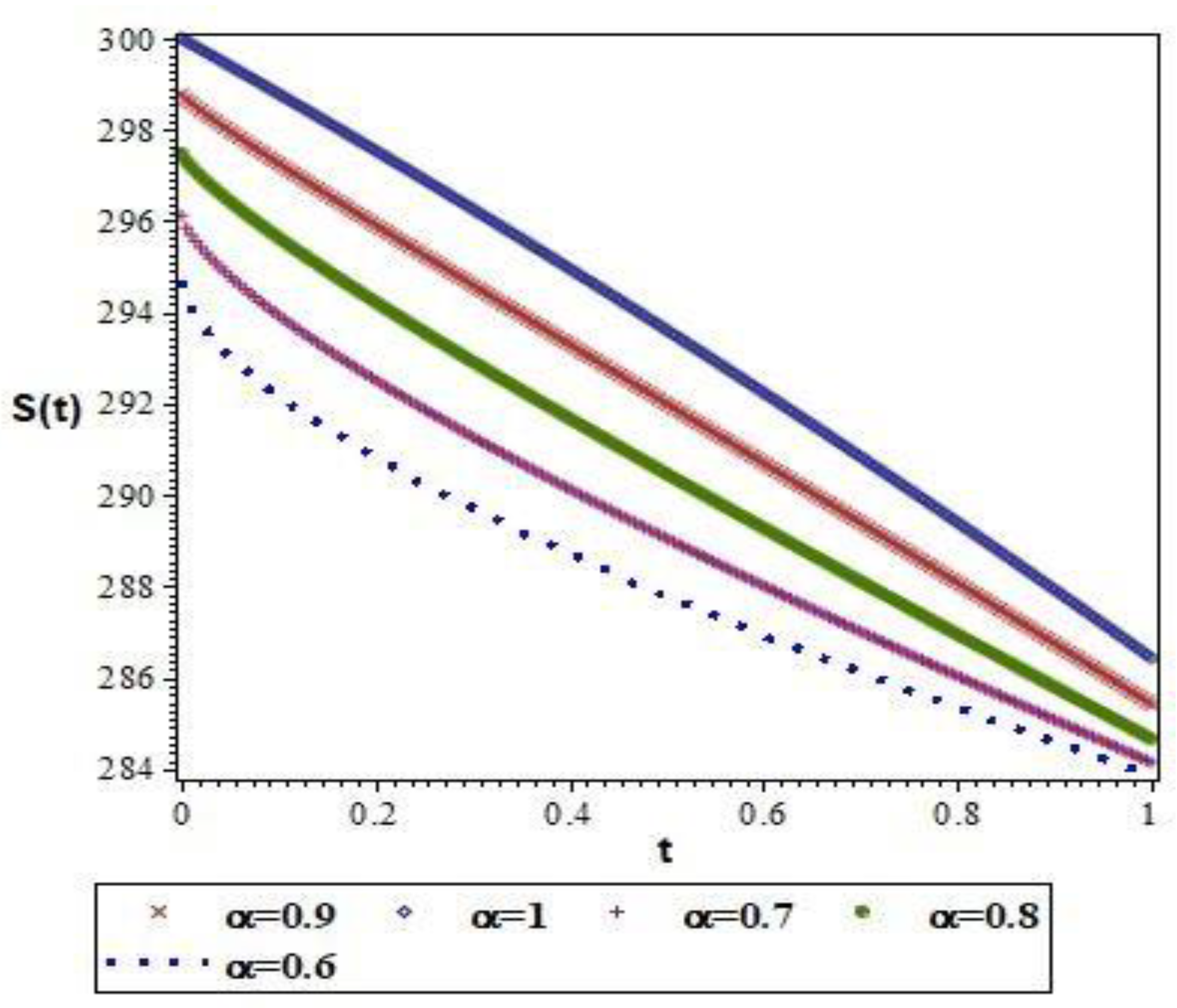
t	α = 0.6	α = 0.7	α = 0.8	α = 0.9	α = 1
0.2	290.8332821	292.5215509	294.2312730	295.9169066	297.5450103
0.4	288.7183111	290.1361784	291.6812730	293.3045941	294.9608370
0.6	286.9466815	288.0170780	289.2823904	290.7063195	292.2474799
0.8	285.3574883	286.0385706	286.9528908	288.0843841	289.4049390
1	283.8864707	284.1493328	284.6590141	285.4232667	286.4332145

,

Table 2. Table of the exposed class of pine trees E(t) at various values of α.

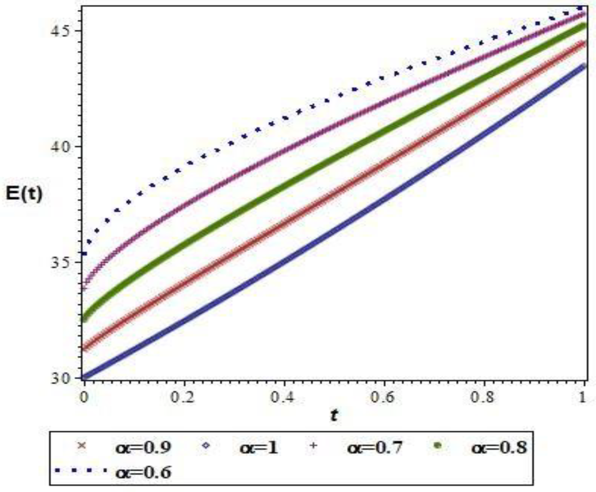
t	α = 0.6	α = 0.7	α = 0.8	α = 0.9	α = 1
0.2	39.10004523	37.42459719	35.72766190	34.05441224	32.43802645
0.4	41.19892275	39.79208318	38.25886843	36.64785418	35.00395898
0.6	42.95693540	41.89509617	40.63981065	39.22704104	37.69779761
0.8	44.53381791	43.85843328	42.95167533	41.82943376	40.51954233
1	45.99336551	45.73306211	45.22800285	44.47046140	43.46919314

,

Table 3. Table of the infective class of pine trees I(t) at various values of α.

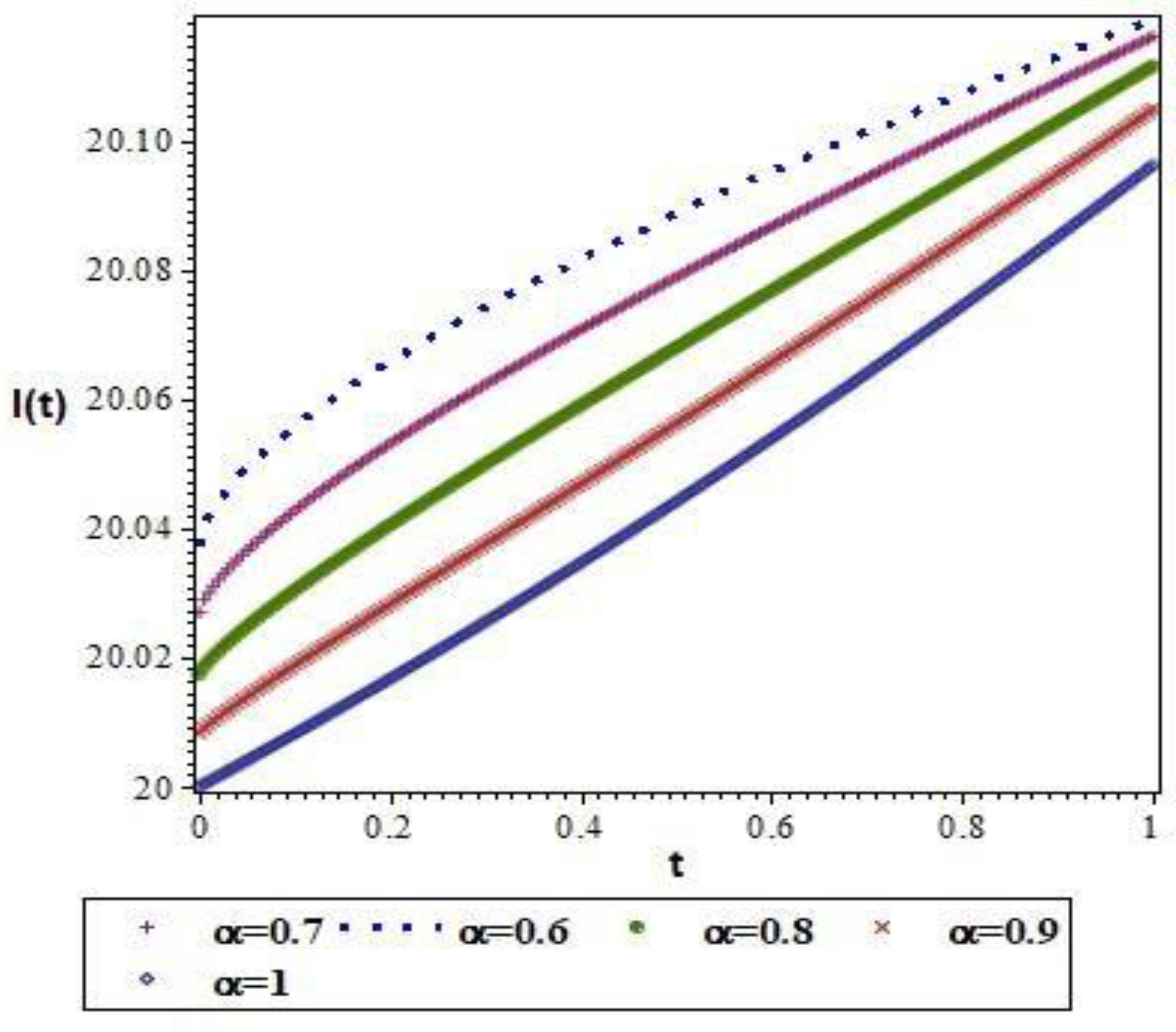
t	α = 0.6	α = 0.7	α = 0.8	α = 0.9	α = 1
0.2	20.06569309	20.05303066	20.04041223	20.02820332	20.01666441
0.4	20.08158972	20.07068416	20.05894326	20.04678947	20.03460646
0.6	20.09504715	20.08657271	20.07664739	20.06560725	20.05382613
0.8	20.10721869	20.10156349	20.09406166	20.08488908	20.07432344
1	20.11856300	20.11600600	20.11140109	20.10472442	20.09609837

,

Table 4. Table of the susceptible class of beetles R(t) at various values of α.

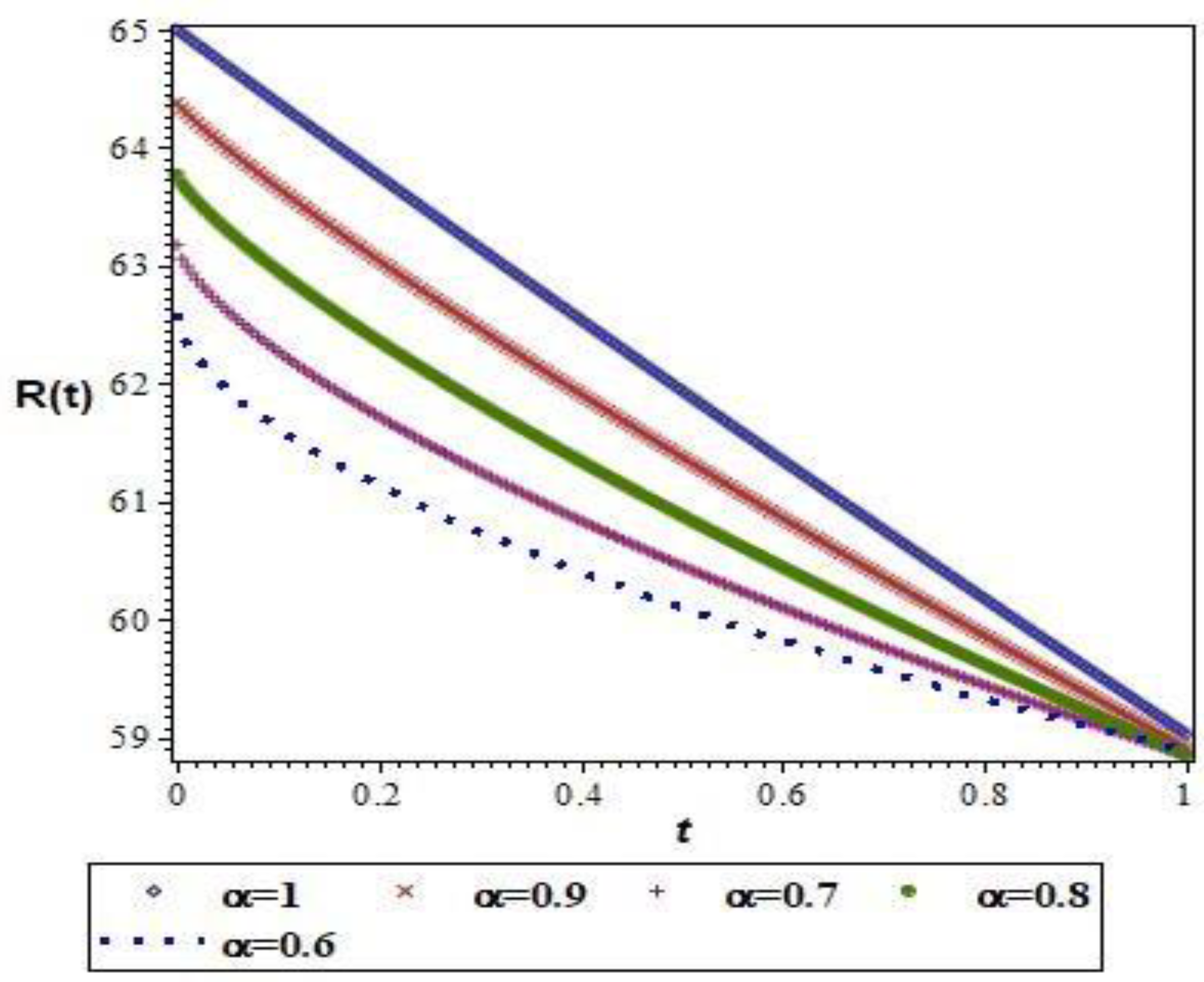
t	α = 0.6	α = 0.7	α = 0.8	α = 0.9	α = 1
0.2	61.13521917	61.72265599	62.36277835	63.04502340	63.75988658
0.4	60.40677303	60.84027518	61.34428024	61.91386799	62.54295352
0.6	59.82779844	60.10177564	60.44600834	60.86194973	61.34920081
0.8	59.33049050	59.44677866	59.62275299	59.86504614	60.17862847
1	58.88735002	58.84960935	58.85433742	58.91180471	59.03123648

and

Table 5. Table of the infective class of beetles Q(t) at various values of α.

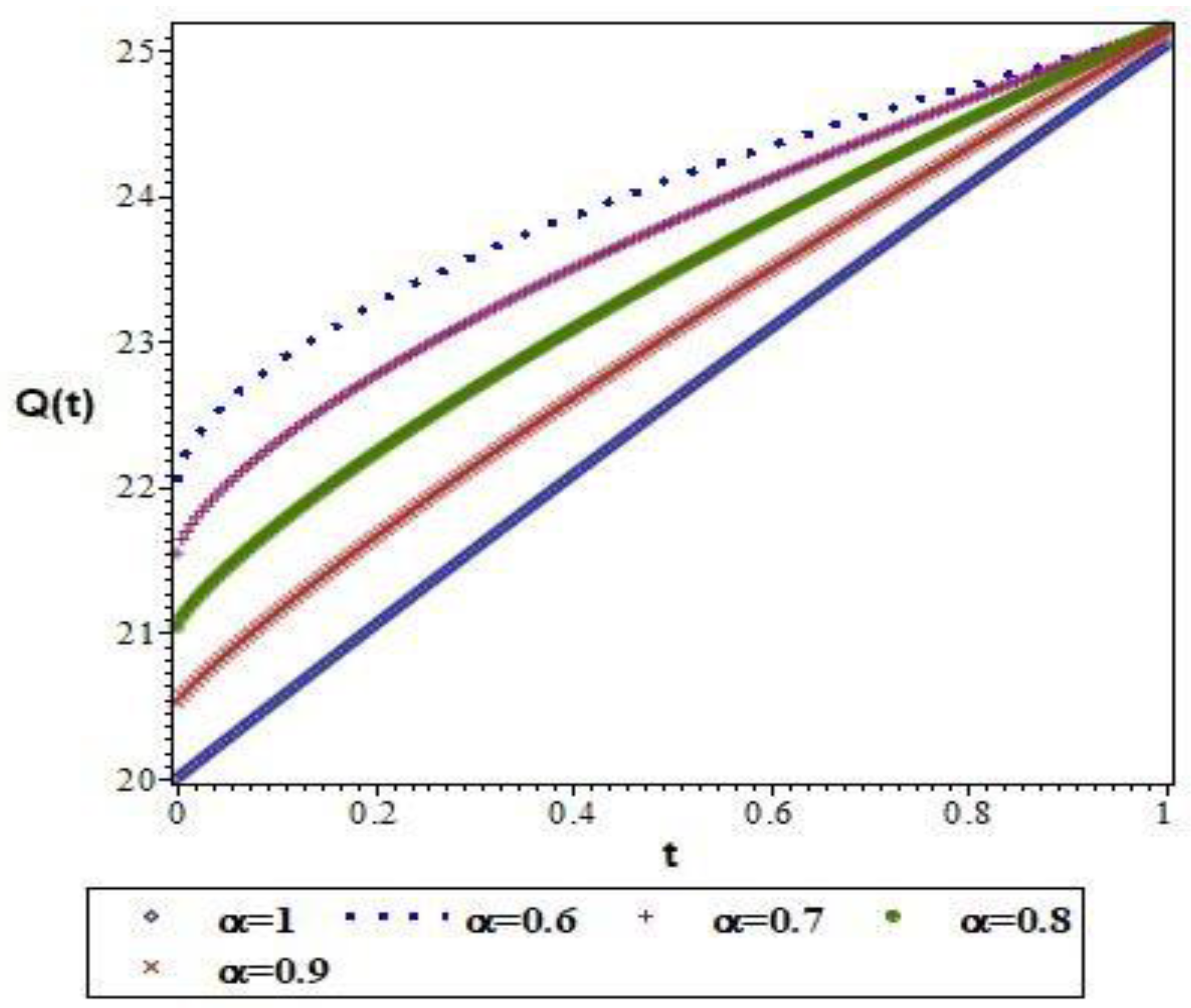
t	α = 0.6	α = 0.7	α = 0.8	α = 0.9	α = 1
0.2	23.25119176	22.76220249	22.22707314	21.65432952	21.05177564
0.4	23.85718191	23.49935245	23.08151053	22.60713914	22.08081457
0.6	24.33723469	24.11414638	23.83245361	23.49023543	23.08711678
0.8	24.74838860	24.65768508	24.51838248	24.32434237	24.07068228
1	25.11379385	25.15173547	25.15651828	25.11921053	25.03151105

show the solution for $S\left(t\right); E\left(t\right); I\left(t\right); R\left(t\right)$; and $Q\left(t\right)$, respectively, for various fractional orders (α) with respect to time (t) obtained by q-HAT. We designate a solution for S(t); E(t); I(t); R(t); and Q(t) in Figure 1, Figure 2, Figure 3, Figure 4 and Figure 5 correspondingly.

Table 1, Table 2, Table 3, Table 4 and Table 5 illustrate the answer to S(t); E(t); I(t); R(t); and Q(t), respectively, acquired by q-HATM. We have chosen inclined values for α to discuss the spread of disease and growth in diseased beetles. One can observe from Table 1 that enhancing values of $\alpha$ with respect to $t$ increases the numerical value of the susceptible class of pine trees. Table 2 depicts the difference in exposed pine trees for varied values of $\alpha$. The exposed pine tree population gradually declines with rising values of $\alpha$ with respect to time. The variation in the infected class of pine trees for diverse values of fractional order changes according to its time, as depicted in Table 3. One can detect from Table 3 that $I\left(t\right)$ gradually or slightly increases with a fixed value of $\alpha$ with respect to a rise in $t$. However, a rise in values of α for a fixed time $t$ declines $I\left(t\right).$ Table 4 is tabulated to discuss the variation in the numerical value of the population of the susceptible class of beetles for distinct values of $\alpha$. It is detected from the table that $R\left(t\right)$ gradually increases for inclined values of $\alpha$ with respect to fixed. The variation in the population of the infective class of beetles for rising values of α with respect to time is tabulated in Table 5. One can observe from the table that an increase in α with respect to a fixed time reduces the numerical value of the population of the infected class of beetles. From the table, we can conclude that the fractional derivative method applied to hypothetical models allows for a noteworthy augmentation in the fitting of genuine information when compared to old-style models.

We interpret the solution by q-HATM for $S\left(t\right), E\left(t\right), I\left(t\right), R\left(t\right), and Q\left(t\right)$ in Figure 1, Figure 2, Figure 3, Figure 4 and Figure 5, correspondingly. Figure 1 displays the pictural illustration of the exact simulation for susceptible pine trees S(t) in a time t for diverse values of $\alpha$ at $h=-1$ and $n=1$. One can observe from the plotted figure that the susceptible population of pine wilt trees increases for a rise in values of $\alpha$ with respect to time $t$. Here, $S\left(t\right)$ acts as an increasing function of $t$. The visual appearance of the analytical scheme for the exposed class of pine tree in a time t for changed $\alpha$ at $h=-1$ and $n=1$ is displayed in Figure 2. It is evident from the plotted graph that an increase in α with respect to time decreases the exposed class of pine trees. Further, E(t) acts as increasing function of t for a fixed α. Figure 3 shows a visual depiction of the numerical solution for the infective class of pine tree $I\left(t\right)$ in time t for different values of $\alpha$ at $h=-1$ and $n=1$. One can detect from the plotted graph that a rise in values of $\alpha$ increases the infective class of pine trees. Here, $I\left(t\right)$ acts as increasing function of $t$ for a fixed $\alpha$. To verify the characteristic feature of susceptible pine trees at various fractional orders at h = −1 and n = 1, Figure 4 is portrayed. For an inclined fractional order, it is observed that the population of susceptible pine trees grows. Furthermore, $R\left(t\right)$ acts as a deceasing function of t for a fixed $\alpha$. One can observe that the fractional differential co-efficient order at $h=-1$ and $n=1$ enhances the rate of growth in the infective class of beetles, as revealed in Figure 5. Here, Q(t) acts as an increasing function of t for a fixed $\alpha$.

7. Conclusions

The productive model of pine wilt disease inside the complicated structure of fractional calculus is analyzed using the q-Homotopy Analysis Transform Method. The results of the model analysis revealed that the approach and fractional operator are particularly useful in analyzing real-world scenarios. Furthermore, the current method saves time and does not require any deviation while solving nonlinear models. It is concluded that the considered nonlinear model can be used to derive results for existent, non-existent, and other phenomenal factors.

References

- Mamiya, Y. Pathology of the Pine Wilt Disease Caused by Bursaphelenchus xylophilus. Annu. Rev. Phytopathol. 1983, 21, 201–220. [Google Scholar] [CrossRef] [PubMed]
- Mamiya, Y. History of pine wilt disease in Japan. J. Nematol. 1988, 20, 219–226. [Google Scholar] [PubMed]
- Fukuda, K. Physiological Process of the Symptom Development and Resistance Mechanism in Pine Wilt Disease. J. For. Res. 1997, 2, 171–181. [Google Scholar] [CrossRef]
- Proenca, D.N.; Gregor, G.; Morais, P.V. Understanding pine wilt disease: Roles of the pine endophytic bacteria and of the bacteria carried by the disease-causing pine wood nematode. Mic. Biol. Open 2016, 6, e00415. [Google Scholar] [CrossRef]
- Ozair, M.; Hussain, T.; Awan, A.U.; Aslam, A.; Khan, R.A.; Ali, F.; Tasneem, F. Bio-inspired analytical heuristics to study pine wilt disease model. Sci. Rep. 2020, 10, 3534. [Google Scholar] [CrossRef]
- Awan, A.U.; Ozair, M.; Din, Q.; Hussain, T. Stability analysis of pine wilt disease model by periodic use of insecticides. J. Biol. Dyn. 2016, 10, 506–524. [Google Scholar] [CrossRef] [Green Version]
- Lee, K.S.; Lashari, A.A. Global Stability of a Host-Vector Model for Pine Wilt Disease with Nonlinear Incidence Rate. Abstr. Appl. Anal. 2014, 2014, 219173. [Google Scholar] [CrossRef] [Green Version]
- Lee, K.S.; Lashari, A.A. Stability analysis and optimal control of pine wilt disease with horizontal transmission in vector population. Appl. Math. Comput. 2014, 226, 793–804. [Google Scholar] [CrossRef]
- Takasu, F. Individual-based modeling of the spread of pine wilt disease: Vector beetle dispersal and the Allee effect. Popul. Ecol. 2009, 51, 399–409. [Google Scholar] [CrossRef]
- Pathak, S.; Maiti, A.; Samanta, G. Rich dynamics of an SIR epidemic model. Nonlinear Anal. Model. Control 2010, 15, 71–81. [Google Scholar] [CrossRef]
- Shi, X.; Song, G. Analysis of the Mathematical Model for the Spread of Pine Wilt Disease. J. Appl. Math. 2013, 2013, 184054. [Google Scholar] [CrossRef]
- Lia, Y.; Haq, F.; Shah, K.; Shahzad, M.; Rahman, G. Numerical analysis off ractional order pine wilt disease model with bilinear incident rate. J. Math. Comput. Sci. 2017, 17, 420–428. [Google Scholar] [CrossRef] [Green Version]
- Rahman, G.U.; Shah, K.; Haq, F.; Ahmad, N. Host vector dynamics of pine wilt disease model with convex incidence rate. Chaos Solitons Fractals 2018, 113, 31–39. [Google Scholar] [CrossRef]
- Shah, K.; Alqudah, M.A.; Jarad, F.; Abdeljawad, T. Semi-analytical study of Pine Wilt Disease model with convex rate under Caputo–Febrizio fractional order derivative. Chaos Solitons Fractals 2020, 135, 109754. [Google Scholar] [CrossRef]
- Atkins, D.; Davis, T.S.; Stewart, J.E. Pine Wilt Disease in the Front Range; Colorado State University: Fort Collins, CO, USA, 2020. [Google Scholar]
- Alkahtani, B.S.T.; Atangana, A. Analysis of non-homogeneous heat model with new trend of derivative with fractional order. Chaos Solitons Fractals 2016, 89, 566–571. [Google Scholar] [CrossRef]
- Atangana, A.; Gómez-Aguilar, J. Fractional derivatives with no-index law property: Application to chaos and statistics. Chaos Solitons Fractals 2018, 114, 516–535. [Google Scholar] [CrossRef]
- Atangana, A.; Gomez-Aguilar, J.F. A new derivative with normal distribution kernal: Theory, methods and applications. Phys. A 2017, 476, 1–14. [Google Scholar] [CrossRef]
- Atangana, A.; Gomez-Aguilar, J.F. Hyperchaotic behavior obtained via a nonlocal operator with exponential decay and Mittag-Leffler laws. Chaos Solitons Fractals 2017, 102, 285–294. [Google Scholar] [CrossRef]
- Caputo, M. Elasticita e Dissipazione; Zanichelli: Bologna, Italy, 1969. [Google Scholar]
- Gomez-Aguilar, J.F.; Atangana, A.; Morales-Delgado, V.F. Electrical circuits RC, LC and RL described by Atangana-Baleanu fractional derivatives. Int. J. Circ. Theor. Appl. 2017, 45, 1514–1533. [Google Scholar] [CrossRef]
- Gomez-Aguilar, J.F.; Baleanu, D. Fractional transmission line with losses. Z. Nat. A 2014, 69, 539–546. [Google Scholar] [CrossRef] [Green Version]
- Gomez-Aguilar, J.F.; Torres, L.; Yepez-Martinez, H.; Baleanu, D.; Reyes, J.M.; Sosa, I.O. Fractional Lie nard type model of a pipe line with in the fractional derivative without singular kernel. Adv. Differ. Eq. 2016, 2016, 173. [Google Scholar] [CrossRef] [Green Version]
- Miller, K.S.; Ross, B. An Introduction to the Fractional Calculus and Fractional Differential Equations; John Wiley & Sons, Inc.: New York, NY, USA, 1993. [Google Scholar]
- Owolabi, K.M.; Atangana, A. Mathematical analysis and computational experiments for an epidemic system with non-local and non-singular derivative. Chaos Solitons Fractals 2019, 126, 41–49. [Google Scholar] [CrossRef]
- Prakash, A.; Kaur, H. Analysis and numerical simulation of fractional order Chan-Allen model with Atangana-Baleanu derivatives. Chaos Solitons Fractals 2019, 124, 134–142. [Google Scholar] [CrossRef]
- Prakasha, D.G.; Veeresha, P. Analysis of Lakes Pollution Model with Mittag-Leffler Kernal. J. Ocean. Eng. Sci. 2020, 5, 310–322. [Google Scholar] [CrossRef]
- Padmavathi, V.; Prakash, A.; Alagesan, K.; Magesh, N. Analysis and numerical simulation of novel corona virus (COVID-19) model with Mittag-Leffler Kernel. Math. Meth. Appl. Sci. 2020, 44, 1863–1877. [Google Scholar] [CrossRef]
- Prakash, A.; Kaur, H. Numerical solution for fractional model of Fokker-Planck equation by using q-HATM. Chaos Solitons Fractals 2017, 105, 99–110. [Google Scholar] [CrossRef]
- Singh, J.; Kumar, D.; Baleanu, D. New aspects of fractional Biswas-Milivic model with Mittag-Leffler law. Math. Model. Nat. Phenom. 2019, 14, 303. [Google Scholar] [CrossRef] [Green Version]
- Prakash, A.; Goyal, M.; Baskonus, H.M.; Gupta, S. A reliable hybrid numerical method for a time dependent vibration model of arbitrary order. AIMS Math. 2020, 5, 979–1000. [Google Scholar] [CrossRef]