Orientational Sampling Schemes Based on Four Dimensional Polytopes

Abstract

The vertices of regular four-dimensional polytopes are used to generate sets of uniformly distributed three-dimensional rotations, which are provided as tables of Euler angles. The spherical moments of these orientational sampling schemes are treated using group theory. The orientational sampling sets may be used in the numerical computation of solid-state nuclear magnetic resonance spectra, and in spherical tensor analysis procedures.

1. Introduction

In general, physical properties are anisotropic, meaning that they depend on the orientation of the object of interest in three-dimensional space, defined with respect to an external reference frame. For example, the magnetic resonance response of solid samples depends on the orientation of the molecules with respect to the applied magnetic field [1,2]. Similar considerations apply to many other physical quantities and spectroscopic properties.

If the physical system is macroscopically isotropic (for example, a finely-divided powdered solid), all molecular orientations are encountered with equal probability. The physical response of such systems is an average over all molecular orientations.

Suppose that a computational method exists for estimating the value of a particular macroscopic observable for a single molecular orientation. To estimate the powder response, it is necessary to average the results of such computations over a large number of distinct orientations. This is called powder averaging, and is a common procedure in, for example, the computation of solid-state magnetic resonance observables [3,4,5,6]. In general, the computational cost of powder averaging is proportional to the number of sampled orientations. It is clearly desirable to use an orientational sampling scheme that gives an acceptable approximation to the isotropic result using the minimum number of orientations. The problem of optimum orientational sampling has been a recurring feature of the solid-state nuclear magnetic resonance (NMR) literature for many years [3,4,5,6].

In addition, there are experimental procedures that require repetition of an experiment for a set of different physical orientations of the system (or parts of the system), in order to estimate the values of anisotropic physical quantities. Physical manipulations of this kind are found, for example, in the NMR of microscopically oriented samples such as single crystals or oriented materials [1].

There are also experiments of this type in which the sample remains fixed in space, but the orientations of the nuclear spin polarizations are manipulated using applied radio-frequency pulse sequences. For example, in the class of experiments known as spherical tensor analysis [7,8,9], the orientational space of the nuclear spins is sampled in order to derive the spherical tensor components of the quantum statistical operator describing the state of the nuclear spin ensemble. In all such experimental procedures, it is desirable that the orientation sampling scheme is as efficient as possible.

1.1. Gaussian Spherical Quadrature

An approach to the orientational sampling problem, using the concept of Gaussian spherical quadrature, was described by Edén et al. in 1998 [4]. This approach may be summarized as follows: An orientational sampling scheme $\mathcal{S}$ consists of a finite set ${\mathsf{\Omega }}^{\mathcal{S}}$ of ${\mathcal{N}}_{\mathcal{S}}$ distinct orientations ${\mathsf{\Omega }}_j^{\mathcal{S}}$ in three-dimensional space, and a set ${\mathbf{w}}^{\mathcal{S}}$ of weights$w_j^{\mathcal{S}}$ with the property ${\sum }_{j=1}^{{\mathcal{N}}_{\mathcal{S}}}{w}_j^{\mathcal{S}}=1$. Both sets have the same number of elements ${\mathcal{N}}_{\mathcal{S}}$. The isotropic average $〈Q〉$ of a physical observable Q is estimated by computing Q for each orientational sampling point ${\mathsf{\Omega }}_j^{\mathcal{S}}$ and superposing the results according to:

$${〈Q〉}_{\mathrm{est}}^{\mathcal{S}}=\sum _{j=1}^{{\mathcal{N}}_{\mathcal{S}}}{w}_j^{\mathcal{S}}Q\left({\mathsf{\Omega }}_j^{\mathcal{S}}\right)$$

(1)

The performance of a sampling scheme may be characterized by its spherical moments, which are defined as follows:

$${\sigma }_{\ell m{m}^{\prime }}^{\mathcal{S}}=\sum _{j=1}^{{\mathcal{N}}_{\mathcal{S}}}{w}_j^{\mathcal{S}}{D}_{m{m}^{\prime }}^{\ell }\left({\mathsf{\Omega }}_j^{\mathcal{S}}\right)$$

(2)

Here $D_{m{m}^{\prime }}^{\ell }\left({\mathsf{\Omega }}_j^{\mathcal{S}}\right)$ is an element of the Wigner matrix [10] of integer rank ℓ, evaluated at orientation ${\mathsf{\Omega }}_j^{\mathcal{S}}$. The Wigner matrices are representations of the group of the three-dimensional rotations $SO\left(3\right)$, with the Wigner matrices of integer rank ℓ spanning the irreducible representation of $SO\left(3\right)$ of dimension $2\ell +1$. If the rotation ${\mathsf{\Omega }}_j^{\mathcal{S}}$ is parametrized using the three Euler angles $\{{\alpha }_j^{\mathcal{S}},{\beta }_j^{\mathcal{S}},{\gamma }_j^{\mathcal{S}}\}$, representing consecutive rotations about the z, y and z-axes of 3D space, all Wigner matrix elements may be written as follows:

$$D_{m{m}^{\prime }}^{\ell }\left({\mathsf{\Omega }}_j^{\mathcal{S}}\right)={\mathrm{e}}^{-\mathrm{i}{m}^{\prime }{\alpha }_j^{\mathcal{S}}}{d}_{m{m}^{\prime }}^{\ell }\left({\beta }_j^{\mathcal{S}}\right){\mathrm{e}}^{-\mathrm{i}m{\gamma }_j^{\mathcal{S}}}$$

(3)

where $d_{m{m}^{\prime }}^{\ell }\left({\beta }_j^{\mathcal{S}}\right)$ is an element of the reduced Wigner matrix and the indices m and $m^{\prime }$ span the integers in the range $-\ell ,\dots ,\ell$. By definition, the zero-rank spherical moment is given by ${\sigma }_{000}^{\mathcal{S}}=1$.

As discussed by Edén et al. [4], orientational sampling schemes may be constructed which have vanishing spherical moments over a range of ranks, i.e.

$${\sigma }_{\ell m{m}^{\prime }}^{\mathcal{S}}=0\mathrm{for} 1\le \ell \le {\ell }_{\max }^{\mathcal{S}}$$

(4)

Schemes of this kind often provide a good approximation for the isotropic average of an observable Q, using a sampling set $\mathcal{S}$ of relatively small size. Their performance is particularly good if Q is a smooth function of orientation $\mathsf{\Omega }$. This is called Gaussian spherical quadrature since it describes a numerical approach to integration of a function over three-dimensional space that is analogous to Gaussian numerical integration on a line interval. The Wigner functions play the same role as orthogonal polynomials in the case of Gaussian line integration.

In general, sampling schemes with large values of ${\ell }_{\max }^{\mathcal{S}}$ provide a more accurate isotropic average than schemes with small values of ${\ell }_{\max }^{\mathcal{S}}$, but require a larger number of elements ${\mathcal{N}}_{\mathcal{S}}$ for their realization. The central problem in Gaussian spherical quadrature is to achieve large values of ${\ell }_{\max }^{\mathcal{S}}$ with as small ${\mathcal{N}}_{\mathcal{S}}$ as possible.

1.2. Two-angle Sampling and Regular Polyhedra

In many physical situations, the observable of interest Q depends on only two of the three Euler angles defining the orientation in three-dimensional space. This situation arises, for example, in the ordinary NMR of static solids, where the rotational angle of the sample around the static magnetic field has no influence on NMR observables. This is also true for some classes of NMR experiments in rotating solids, as discussed in Reference [4].

Consider an experiment, or computational procedure, of this type, in which the observable of interest does not depend on the third Euler angle $\gamma$. In such cases, the only relevant spherical moments of an orientational sampling scheme have $m^{\prime }=0$. The known relationships between Wigner functions of the type $D_{m0}^{\ell }\left(\mathsf{\Omega }\right)$ and the spherical harmonics $Y_{\ell m}(\theta ,\varphi )$ allows the relevant spherical moments to be written as follows:

$${\sigma }_{\ell m0}^{\mathcal{S}}=\sqrt{\frac{4\pi }{2\ell +1}}\sum _{j=1}^{{\mathcal{N}}_{\mathcal{S}}}{w}_j^{\mathcal{S}}{Y}_{\ell m}{({\beta }_j^{\mathcal{S}},{\alpha }_j^{\mathcal{S}})}^{*}$$

(5)

where ${}^{*}$ means complex conjugation. The problem of two-angle orientational sampling is therefore closely related to the problem of Gaussian quadrature on the surface of a sphere, using spherical harmonics as the orthogonal basis functions. The correspondence of the Euler angles $\{\alpha ,\beta \}$ to the polar angles $\{\theta ,\varphi \}$ of a point on the surface of a sphere is as follows:

$$\begin{array}{c}\hfill \alpha \leftrightarrow \varphi \\ \hfill \beta \leftrightarrow \theta \end{array}$$

(6)

For small values of ${\ell }_{\max }^{\mathcal{S}}$, efficient two-angle sampling schemes may be constructed from the vertices of the regular three-dimensional polyhedra. As discussed below, the point symmetry groups of such polyhedra ensure that many of the spherical moments ${\sigma }_{\ell m0}^{\mathcal{S}}$ vanish. For example, the 12 vertices of the icosahedron may be used to construct an orientational sampling set with ${\mathcal{N}}_{\mathcal{S}}=12$, all $w_j^{\mathcal{S}}=1/12$, and spherical moments ${\sigma }_{\ell m0}^{\mathcal{S}}=0$ for $1\le \ell \le 5$. All spherical moments with odd values of ℓ vanish for this set as well. These favourable properties are well-known in nuclear magnetic resonance and have led to numerous applications [11,12].

It is not possible to construct sampling sets with ${\ell }_{\max }^{\mathcal{S}}>5$ from the vertices of the regular 3D polyhedra. However Lebedev and co-workers [13,14,15] have constructed schemes with large values of ${\ell }_{\max }^{\mathcal{S}}$ by using well-chosen orientational sampling points and non-uniform weights. Alternative methods are also available, which do not have such well-defined mathematical properties, but which perform well in many circumstances, for example the REPULSION approach of Bak and Nielsen, which uses numerical optimization under a repulsive electrostatic potential to distribute many points evenly on the surface of a 3D sphere [3].

1.3. Three-Angle Sampling and Regular 4-Polytopes

There are numerous cases where the observable of interest depends on all three Euler angles defining the orientation $\mathsf{\Omega }$. Some examples from the field of solid-state nuclear magnetic resonance are discussed in Reference [4,5]. In such cases, it is important that the spherical moments ${\sigma }_{\ell m{m}^{\prime }}^{\mathcal{S}}$ vanish for all ${(2\ell +1)}^2$ combinations of m and $m^{\prime }$ within a given rank ℓ, and not just the special components with $m^{\prime }=0$.

As described in Reference [4], it is possible to construct three-angle orientational sampling sets with the appropriate properties by (i) taking a two-angle sampling set with the property ${\sigma }_{\ell m0}^{\mathcal{S}}=0$ for $1\le \ell \le {\ell }_{\max }^{\mathcal{S}}$, and (ii) repeating each sampling point while stepping the third angle through $({\ell }_{\max }^{\mathcal{S}}+1)$ regularly-spaced subdivisions of $2\pi$. This generates a three-angle sampling set with the desired property ${\sigma }_{\ell m{m}^{\prime }}^{\mathcal{S}}=0$ for all $\{m,m^{\prime }\}$ and $1\le \ell \le {\ell }_{\max }^{\mathcal{S}}$. For example, an icosahedral two-angle set with ${\mathcal{N}}_{\mathcal{S}}=12$ may easily be extended to a three-angle set with ${\mathcal{N}}_{\mathcal{S}}=72$ and ${\ell }_{\max }^{\mathcal{S}}=5$. The Lebedev two-angle sets may be extended in analogous fashion. The problems with this approach are (i) it is not efficient, requiring large numbers of orientational samples for modest values of ${\ell }_{\max }^{\mathcal{S}}$ and (ii) it does not treat the Euler angles $\alpha$ and $\gamma$ in the same way.

Since efficient two-angle sampling schemes may be derived from the vertices of regular polyhedra, which fall on a sphere in 3D space, it is natural to speculate that efficient three-angle sampling schemes may be derived from the vertices of regular solids in four dimensions, which fall on a sphere in 4D space. The regular 4D solids are known as regular 4-polytopes or regular polychora [16] and have been studied extensively by mathematicians, in particular Coxeter [17].

Suppose that a 4-polytope is constructed with the vertices lying on the surface of a 4D sphere with unit radius. Each vertex may be converted into a rotation operation in 3D space by identifying it as a unit vector of the following form:

$$\mathbf{q}=\left(\begin{array}{c}\hfill \cos \frac{\xi }{2}\\ \hfill n_x\sin \frac{\xi }{2}\\ \hfill n_y\sin \frac{\xi }{2}\\ \hfill n_z\sin \frac{\xi }{2}\end{array}\right)$$

(7)

where $\xi$ is the rotation angle and $\mathbf{n}=(n_x,n_y,n_z)$ is the unit rotation axis in 3-space, $\mathbf{n}·\mathbf{n}=1$. Hence, uniformly distributed rotations in 3-space may be constructed from the vertices of regular 4-polytopes deducing the corresponding 3D rotation angles and rotation axes from Equation 7. There is one important complication: unit vectors of the form $\mathbf{q}$ and $-\mathbf{q}$ correspond to rotations differing by an angle of $2\pi$, which have the same physical effect on ordinary 3D objects, or on quantum states with integer spin. Hence, a 4-polytope which has the inversion amongst its symmetry operations gives rise to only half the number of physically distinct 3D rotations as its number of vertices. As discussed below, this property applies to all the regular 4-polytopes, with one exception.

Suppose now that a set of N 3D rotations is constructed from the vertices of a regular 4-polytope, and that all of the sampling weights are uniform, $w_j^{\mathcal{S}}=N^{-1}$, $j\in \{1,2\dots N\}$. Many of the spherical moments, defined in Equation 2, are expected to vanish, through symmetry. The question is: for which ranks ℓ do all spherical moments of the form ${\sigma }_{\ell m{m}^{\prime }}^{\mathcal{S}}$ vanish? Although this question has been answered in part using the theory of spherical designs [18], it is also possible to treat this problem by relatively simple group theoretical arguments that may be more accessible to non-mathematicians. However, the application of group theory to this problem is made more difficult by the fact that the symmetry operations of the regular 4-polytopes, and the character tables of the corresponding symmetry groups, are distributed over several sources [19,20,21,22,23]. In this article we collate the symmetry operations and their characters for the regular 4-polytopes in the ${(2\ell +1)}^2$-dimensional representations spanned by the Wigner matrices $D^{\ell }\left(\mathsf{\Omega }\right)$. We derive by group theory the vanishing spherical moments for 3D rotation sets derived from each of the regular 3D and 4D solids. Explicit tables of Euler angles are given, based on the vertices of the regular 4-polytopes. These results should be useful for workers in a wide range of physical sciences, especially magnetic resonance, where one such scheme is already in use [9,24].

2. Group Theory and Symmetry Averaging

2.1. Groups, Representations and Characters

A minimal introduction to group theory is now given in order to establish the notation. For more details, consult the standard texts, for example [25,26,27,28].

An abstract group $\{\mathcal{G},\circ \}$ is a collection of elements G for which a particular associative operation ∘ combines any two elements to give another element in the group. A valid group must include an identity element E such that $G\circ E=G$, and all elements must have an inverse $G^{-1}$ such that $G\circ G^{-1}=E$. Any subset of a group which itself satisfies the group axioms above is called a subgroup.

Groups can be represented by matrices. An n-dimensional linear representation $\mathrm{\Gamma }$ of a group $\mathcal{G}$ assigns an invertible $n\times n$ (real or complex) matrix $M^{\mathrm{\Gamma }}\left(G\right)$ to each group element G, so that the group operation ∘ corresponds to the operation of matrix multiplication:

$$M^{\mathrm{\Gamma }}\left(G_1\circ G_2\right)=M^{\mathrm{\Gamma }}\left(G_1\right)·M^{\mathrm{\Gamma }}\left(G_2\right)$$

(8)

A representation is said to be irreducible if it is not possible to find a basis in which all the matrix representatives of the group elements have the same block diagonal form.

The explicit matrix representations $M^{\mathrm{\Gamma }}\left(G\right)$ are dependent on the choice of the basis vectors. However, for a given representation $\mathrm{\Gamma }$, the characters, defined as the traces of the matrix representations

$${\chi }^{\mathrm{\Gamma }}\left(G\right)=\mathrm{Tr}\left\{M^{\mathrm{\Gamma }}\left(G\right)\right\}$$

(9)

are independent of the basis. Two group elements G and $G^{\prime }$ are said to belong to the same class$\mathcal{C}$ if they are related through a similarity transformation of the form $G=A{G}^{\prime }{A}^{-1}$ where A also belongs to the group $\mathcal{G}$. All elements in the same class have the same character for all representations $\mathrm{\Gamma }$, i.e.

$${\chi }^{\mathrm{\Gamma }}\left(G\right)={\chi }_{\mathcal{C}}^{\mathrm{\Gamma }}\mathrm{for} \mathrm{all} G\in \mathcal{C}$$

(10)

2.2. Subgroup Averaging

Suppose now that the group $\mathcal{G}$ contains a finite subgroup $\mathfrak{g}$ containing $h\left(\mathfrak{g}\right)$ elements. A representation $\mathrm{\Gamma }$ of the group $\mathcal{G}$ is also a representation of the subgroup $\mathfrak{g}$. The finite group orthogonality theorem [28] implies that the number of independent linear combinations of basis vectors spanning the representation $\mathrm{\Gamma }$ which are invariant under all of the subgroup operations $G\in \mathfrak{g}$ is given by

$$a^{\mathrm{\Gamma }}\left(\mathfrak{g}\right)=h{\left(\mathfrak{g}\right)}^{-1}\sum _{G\in \mathfrak{g}}{\chi }^{\mathrm{\Gamma }}\left(G\right)=h{\left(\mathfrak{g}\right)}^{-1}\sum _{\mathcal{C}}{h}_{\mathcal{C}}\left(\mathfrak{g}\right){\chi }_{\mathcal{C}}^{\mathrm{\Gamma }}$$

(11)

where $h_{\mathcal{C}}\left(\mathfrak{g}\right)$ is the number of elements of $\mathfrak{g}$ that belong to the class $\mathcal{C}$. The last two formulations on the right-hand side of 11 are equivalent since all elements in the same class have the same character. This equation leads to the following property:

$$\sum _{\mathcal{C}}{h}_{\mathcal{C}}\left(\mathfrak{g}\right){\chi }_{\mathcal{C}}^{\mathrm{\Gamma }}=0\Rightarrow \sum _{G\in \mathfrak{g}}{M}^{\mathrm{\Gamma }}\left(G\right)=0$$

(12)

The sum of matrices in the representation $\mathrm{\Gamma }$ vanishes if the characters sum to zero over all classes of $\mathfrak{g}$, taking into account the number of subgroup elements $h_{\mathcal{C}}\left(\mathfrak{g}\right)$ in each class.

2.3. Average of a Function in n-dimensional Space

Consider now the case where the group elements G are transformations acting on the points $\mathbf{x}=\{x_1,x_2\dots x_n\}$ of the n-dimensional real space ${\mathbb{R}}^n$, i.e.

$$G\mathbf{x}={\mathbf{x}}^{\prime }$$

(13)

For each group element G, there exists a corresponding operator $\widehat{G}$ acting on functions of the coordinate vectors $f\left(\mathbf{x}\right)$ to generate new functions $f^{\prime }\left(\mathbf{x}\right)$, defined as follows:

$$f^{\prime }\left(\mathbf{x}\right)=\widehat{G}f\left(\mathbf{x}\right)=f\left(G^{-1}\mathbf{x}\right)$$

(14)

The definition above corresponds to an active transformation of the object f [28].

The average function over a finite subgroup $\mathfrak{g}$ of $\mathcal{G}$ is defined by

$${〈f〉}_{\mathfrak{g}}=h{\left(\mathfrak{g}\right)}^{-1}\sum _{G\in \mathfrak{g}}\widehat{G}f$$

(15)

where the sum is taken over all $h\left(\mathfrak{g}\right)$ elements $G\in \mathfrak{g}$ and the same argument $\mathbf{x}$ is implied on both sides of the equation.

Now suppose we have a set of m functions $f_1^{\mathrm{\Gamma }},\dots ,f_m^{\mathrm{\Gamma }}$ forming a basis for an m-dimensional representation $\mathrm{\Gamma }$ of $\mathcal{G}$. Any operator $\widehat{G}$ is then represented by an $m\times m$ matrix $M^{\mathrm{\Gamma }}\left(G\right)$ acting on the set of basis functions from the right [29]:

$$\widehat{G}{f}_i^{\mathrm{\Gamma }}\left(\mathbf{x}\right)=\sum _j{f}_j^{\mathrm{\Gamma }}\left(\mathbf{x}\right)M_{ji}^{\mathrm{\Gamma }}\left(G\right)$$

(16)

Equation 12 gives a sufficient condition for the average of each $f_i^{\mathrm{\Gamma }}$ function to vanish:

$$\sum _{\mathcal{C}}{h}_{\mathcal{C}}\left(\mathfrak{g}\right){\chi }_{\mathcal{C}}^{\mathrm{\Gamma }}=0\Rightarrow {〈f_i^{\mathrm{\Gamma }}〉}_{\mathfrak{g}}=0$$

(17)

2.4. Average of a Function Over the Polytope Vertices

The average value of a function f over a finite set P of $N_0$ points in the n-dimensional space is defined as follows:

$${〈f〉}_P=N_0^{-1}\sum _{v}f\left({\mathbf{x}}_v\right)$$

(18)

where ${\mathbf{x}}_v$ denote the coordinate vectors of the points for $v\in \left\{1,2\dots ,N_0\right\}$. A group $\mathcal{G}$ of $n-$ dimensional transformations is said to act transitively on the P when for any given pair of points ${\mathbf{x}}_v,{\mathbf{x}}_v^{\prime }\in P$ there is a transformation G which connects such points ${\mathbf{x}}_v^{\prime }=G{\mathbf{x}}_v$ [25].

The orbit stabilizer and Lagrange theorems for finite groups [25] relate the average of a function f over P to the average over any finite group ${\mathfrak{g}}_P$ acting transitively on the set:

$$N_0^{-1}\sum _{v}f\left({\mathbf{x}}_v\right)=h{\left({\mathfrak{g}}_P\right)}^{-1}\sum _{G\in {\mathfrak{g}}_P}f\left(G^{-1}{\mathbf{x}}_1\right)=h{\left({\mathfrak{g}}_P\right)}^{-1}\sum _{G\in {\mathfrak{g}}_P}\widehat{G}f\left({\mathbf{x}}_1\right)$$

(19)

The right-hand side corresponds to Equation 15, evaluated at any point ${\mathbf{x}}_1$ in the set. From Equation 17, the average vanishes if the function f is one of the basis functions of the representation $\mathrm{\Gamma }$, and the characters of the given finite group sum ${\mathfrak{g}}_P$ to zero for that representation:

$$\sum _{\mathcal{C}}{h}_{\mathcal{C}}\left({\mathfrak{g}}_P\right){\chi }_{\mathcal{C}}^{\mathrm{\Gamma }}=0\Rightarrow {〈f_i^{\mathrm{\Gamma }}〉}_P=0$$

(20)

Equation 20 is the central result of this section. The point symmetry group of an n-dimensional regular polytope is a finite group which acts transitively on the polytope vertices. It is a subgroup of the (infinite) orthogonal group $O\left(n\right)$, which is the group of all the n-dimensional space transformations in with a single fixed point and which preserve distance between transformed points. Using Equation 20, the averaging properties of a function over the vertices of a polytope may be deduced from the characters of the symmetry elements and the classes of its symmetry point group. This result is now applied to the spherical moments of the regular solids.

3. Polyhedral Averaging in Three Dimensions

Three dimensional polytopes are known as polyhedra. In this section we discuss the averaging properties of the regular polyhedra with respect to spherical harmonics. Although this topic has been treated before in Reference [11], a recapitulation is useful for framing the discussion of four-dimensional symmetries. In addition, the treatment in Reference [11] did not exploit all the available symmetries, as discussed below.

3.1. Proper and Improper Rotations

The proper rotations in three dimensions may be defined in various ways. For example, the symbol $R_{\mathbf{n}}\left(\xi \right)$ indicates a rotation through the angle $\xi$ about a unit rotation axis $\mathbf{n}$ whose direction is defined by the polar angles $\{\theta ,\varphi \}$. The identity operation $R_{}\left(0\right)$ does not need any specification of the rotation axis. Any rotation in 3D space may be decomposed into the product of three consecutive rotations around the cartesian reference axes, for example: $R_{\mathbf{n}}\left(\xi \right)=R_{\mathbf{z}}\left(\alpha \right)R_{\mathbf{y}}\left(\beta \right)R_{\mathbf{z}}\left(\gamma \right)$, where the rotations are applied in sequence from right to left. For a given rotation R the three Euler angles ${\mathsf{\Omega }}_R=\{\alpha ,\beta ,\gamma \}$ and the set $\{\xi ,\theta ,\varphi \}$ are related [10]. Specifically, the rotation angle $\xi$ is related to the Euler angles as follows:

$$\cos \frac{\xi }{2}=\cos \frac{\beta }{2}\cos \frac{\alpha +\gamma }{2}$$

(21)

The improper rotations in three-dimensional space may be expressed in various ways. In this article, we use the set of improper rotations, denoted ${\tilde{R}}_{\mathbf{n}}\left(\xi \right)$. Each improper rotation corresponds to a proper rotation $R_{\mathbf{n}}\left(\xi \right)$ followed by an inversion through the reference frame origin (roto-inversion). By definition, the inversion operation corresponds to the improper rotation ${\tilde{R}}_{}\left(0\right)$, where the rotation axis does not need to be specified in this case.

Two other improper rotations are often used in the literature: the reflection ${\sigma }_h$ in the plane h, and the roto-reflection $S_m$ which is a rotation through $2\pi /m$ followed by reflection in the plane perpendicular to the rotation axis. Reflections and roto-reflections correspond to improper rotations as follows: ${\sigma }_h={\tilde{R}}_{{\mathbf{n}}^{\prime }}\left(\pi \right)$ where ${\mathbf{n}}^{\prime }$ is perpendicular to the plane h, and $S_m={\tilde{R}}_{{\mathbf{n}}^{″}}(\pi +2\pi /m)$ where ${\mathbf{n}}^{″}$ is the rotation axis defined by $S_m$ for $m\ge 3$. Clearly $S_2={\tilde{R}}_{}\left(0\right)$ and $S_1={\tilde{R}}_{{\mathbf{n}}^{″}}\left(\pi \right)$.

3.2. Representations and Characters of $O\left(3\right)$ Isometries

The set of $2\ell +1$ spherical harmonics of rank-ℓ is defined as follows:

$$Y_{\ell m}(\mathsf{\Theta },\mathsf{\Phi })=\sqrt{\frac{2\ell +1}{4\pi }\frac{(\ell -m)!}{(\ell +m)!}}{P}_{\ell }^m\left(\cos \mathsf{\Theta }\right)e^{\mathrm{i}m\mathsf{\Phi }}$$

(22)

where ℓ and m are integers with $\left|m\right|\le \ell$ and $P_{\ell }^m$ is the associated Legendre polynomial [10]. This set of functions is a basis for the $(2\ell +1)$-dimensional irreducible representation of the $O\left(3\right)$ group. The action of any $O\left(3\right)$ operation G on these functions defines an operator $\widehat{G}$ which is represented by a $(2\ell +1)\times (2\ell +1)$ matrix $M^{\ell }\left(G\right)$:

$$\widehat{G}{Y}_{\ell m}(\mathsf{\Theta },\mathsf{\Phi })=\sum _{m^{\prime }}{Y}_{\ell m^{\prime }}(\mathsf{\Theta },\mathsf{\Phi })M_{m^{\prime }m}^{\ell }\left(G\right)$$

(23)

In the case of a proper rotation R, the matrix representative is given by the rank-ℓ Wigner matrix:

$$M^{\ell }\left(R\right)=D^{\ell }\left({\mathsf{\Omega }}_R\right)$$

(24)

In the case of an improper rotation $\tilde{R}$, the sign of the matrix changes for odd rank ℓ:

$$M^{\ell }\left(\tilde{R}\right)={(-1)}^{\ell }{D}^{\ell }\left({\mathsf{\Omega }}_R\right)$$

(25)

The character of a proper rotation for the rank-ℓ representation is equal to the trace of the corresponding Wigner matrix, ${\chi }_D^{(\ell )}$, which depends on the rotation angle $\xi$ only [10, pp. 99–100]:

$${\chi }^{(\ell )}\left\{R_{\mathbf{n}}\left(\xi \right)\right\}={\chi }_D^{(\ell )}\left(\xi \right)$$

(26)

where

$${\chi }_D^{(\ell )}\left(\xi \right)=\frac{\sin \left\{(2\ell +1)\frac{\xi }{2}\right\}}{\sin \frac{\xi }{2}}$$

(27)

This evaluates to ${\chi }_D^{(\ell )}\left(\xi \right)=2\ell +1$ when the rotation angle $\xi$ is an integer multiple of $2\pi$.

The character of an improper rotation is the same as for the corresponding proper rotation, but with a change in sign for odd values of ℓ:

$${\chi }^{(\ell )}\left\{{\tilde{R}}_{\mathbf{n}}\left(\xi \right)\right\}={(-1)}^{\ell }{\chi }_D^{(\ell )}\left(\xi \right)$$

(28)

3.3. Regular Convex Polyhedra

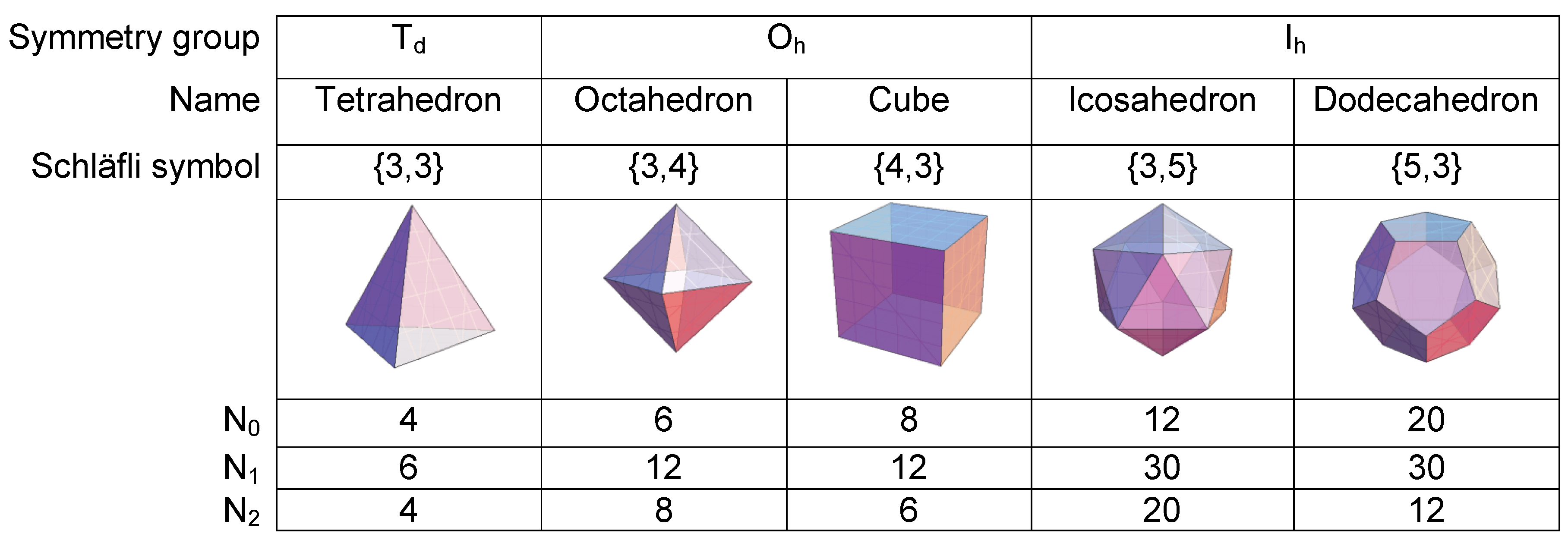
The five regular convex polyhedra have been known since the Greeks. Their names and properties are listed in Figure 1. This figure also provides the Schläfli symbols [17] of the form $\{p,q\}$, where p indicates the number of edges of the regular polygonal face, and q is the number of faces meeting at one vertex. For example, the cube has Schläfli symbol $\{4,3\}$, while the regular octahedron has the Schläfli symbol $\{3,4\}$. Polyhedra with Schläfli symbols $\{p,q\}$ and $\{q,p\}$ are geometrical reciprocals of each other and belong to the same symmetry group, since the reciprocation operation corresponds to the mutual exchange of faces and vertices. The five Platonic solids therefore belong to only three symmetry point groups: (i) $T_d$, represented by the tetrahedron; (ii) $O_h$, populated by the cube and the octahedron; and (iii) $I_h$, populated by the icosahedron and the dodecahedron. The symmetry point groups of the regular polyhedra are given explicitly in

Table 1. The three symmetry point groups of the regular polyhedra. h is the number of symmetry elements in the group. The last column shows the number of elements in each class (in square parentheses), followed by a single symmetry element of the class, for a polyhedron in standard orientation. The symbol $R_{(a,b,c)}\left(\xi \right)$ indicates a rotation through the angle $\xi$ about the axis $(a,b,c)$. The symbol ${\tilde{R}}_{(a,b,c)}\left(\xi \right)$ indicates the improper operation constructed by the proper rotation $R_{(a,b,c)}\left(\xi \right)$ followed by the inversion operation. $R_{}\left(0\right)$ is the identity operation and ${\tilde{R}}_{}\left(0\right)$ is the inversion operation. The symbol $\tau =2\cos (\pi /5)=(\sqrt{5}+1)/2$ indicates the golden ratio.

Symmetry group	h	Symmetry operations
$T_d$	24	$\left[1\right]R\left(0\right);\left[8\right]R_{(1,1,1)}(2\pi /3);\left[3\right]R_{(1,0,0)}\left(\pi \right);$ $\left[6\right]{\tilde{R}}_{(1,0,0)}(\pi /2);\left[6\right]{\tilde{R}}_{(1,1,0)}\left(\pi \right)$
$O_h$	48	$\left[1\right]R\left(0\right);\left[8\right]R_{(1,1,1)}(2\pi /3);\left[3\right]R_{(1,0,0)}\left(\pi \right);$ $\left[6\right]R_{(1,0,0)}(\pi /2);\left[6\right]R_{(1,1,0)}\left(\pi \right);$ $\left[1\right]\tilde{R}\left(0\right);\left[8\right]{\tilde{R}}_{(1,1,1)}(2\pi /3);\left[3\right]{\tilde{R}}_{(1,0,0)}\left(\pi \right);$ $\left[6\right]{\tilde{R}}_{(1,0,0)}(\pi /2);\left[6\right]{\tilde{R}}_{(1,1,0)}\left(\pi \right);$
$I_h$	120	$\left[1\right]R\left(0\right);\left[12\right]R_{(1,0,0)}(2\pi /5);\left[12\right]R_{(1,0,0)}(4\pi /5);$ $\left[20\right]R_{(2,0,{\tau }^2)}(2\pi /3);\left[15\right]R_{(\tau ,0,1)}\left(\pi \right);$ $\left[1\right]\tilde{R}\left(0\right);\left[12\right]{\tilde{R}}_{(1,0,0)}(2\pi /5);\left[12\right]{\tilde{R}}_{(1,0,0)}(4\pi /5);$ $\left[20\right]{\tilde{R}}_{(2,0,{\tau }^2)}(2\pi /3);\left[15\right]{\tilde{R}}_{(\tau ,0,1)}\left(\pi \right);$

.

3.4. Spherical Moments of the Regular Polyhedra

The theorem in Equation 20 may be used with Table 1 and the characters given in Equations 26 and 28 to deduce the vanishing spherical moments of the regular polyhedra. In general, both improper and proper rotations must be taken into account. The treatment in Reference [11] uses only the proper rotations, and gives slightly different results for the groups $O_h$ and $I_h$ (see below).

As a first example, consider the tetrahedron. As shown in Table 1, the tetrahedron has three symmetry classes of proper rotations, with number of elements $(1,8,3)$ and rotation angles $(0,2\pi /3,\pi )$ respectively. In addition, there are two symmetry classes of improper rotations, with number of elements $(6,6)$ and rotation angles $(\pi /2,\pi )$ respectively. The sum of characters for rank $\ell =2$ is therefore given by

$$\begin{array}{ccc}\hfill \sum _{\mathcal{C}}{h}_{\mathcal{C}}\left(T_d\right){\chi }_{\mathcal{C}}^{\left(2\right)}& =& {\chi }_D^{\left(2\right)}\left(0\right)+8{\chi }_D^{\left(2\right)}\left(2\pi /3\right)+3{\chi }_D^{\left(2\right)}\left(\pi \right)+6{(-1)}^2{\chi }_D^{\left(2\right)}\left(\pi /2\right)+6{(-1)}^2{\chi }_D^{\left(2\right)}\left(\pi \right)\hfill \\ & =& 0\hfill \end{array}$$

(29)

This proves the well-known fact that a tetrahedron averages second-rank spherical harmonics to zero:

$${\sigma }_{2m0}\left(T_d\right)=0$$

(30)

The point symmetry groups of the octahedron and icosahedron contain the inversion element. Each proper rotation is therefore accompanied by an improper rotation through the same angle, as shown in Table 1. It follows that all odd-rank spherical moments harmonics vanish when summed over the vertices of polyhedra with symmetries $O_h$ and $I_h$:

$$\begin{array}{ccc}\hfill \sum _{\mathcal{C}}{h}_{\mathcal{C}}\left(O_h\right){\chi }_{\mathcal{C}}^{(\ell )}=\sum _{\mathcal{C}}{h}_{\mathcal{C}}\left(I_h\right){\chi }_{\mathcal{C}}^{(\ell )}& =& 0(\mathrm{for} \mathrm{odd} \ell )\hfill \end{array}$$

(31)

and hence

$${\sigma }_{\ell m0}\left(O_h\right)={\sigma }_{\ell m0}\left(I_h\right)=0(\mathrm{for} \mathrm{odd} \ell )$$

(32)

The treatment of Reference [11] does not predict this result, since only proper rotations were taken into account. The two analyses differ for rank $\ell =9$ and all odd ranks $\ell \ge 13$.

Figure 2 summarizes the spherical rank profiles of the regular convex polyhedra up to rank $\ell =30$. Note that even the most symmetrical polyhedra (the icosahedron and the dodecahedron) fail to average the rank $\ell =6$ terms.

There are 4 regular non-convex polyhedra (star-polyhedra), which all fall in the group $I_h$ [17]. Four of them have the same vertices of the icosahedron while one has the same vertices as the dodecahedron. All have the same spherical moment characteristics as the icosahedron.

4. Polytopic Averaging in Four Dimensions

In this section we derive the spherical averaging properties of the regular 4-polytopes. In the discussion below, we make extensive use of quaternions [29]. As shown in Equation 7, quaternions provide a correspondence between points on a unit sphere in four-dimensional space, and the group of three-dimensional rotations.

4.1. Quaternions

Four-dimensional real space is a vector space: any two vectors can be added or multiplied by a scalar to give another vector. Quaternions extend the vectorial structure of 4D real space by allowing the multiplication of two 4D vectors $\mathbf{q}\left(1\right)$ and $\mathbf{q}\left(2\right)$ according to

$$\left(\begin{array}{c}{q}_1\left(2\right)\\ q_2\left(2\right)\\ q_3\left(2\right)\\ q_4\left(2\right)\end{array}\right)\ast \left(\begin{array}{c}{q}_1\left(1\right)\\ q_2\left(1\right)\\ q_3\left(1\right)\\ q_4\left(1\right)\end{array}\right)=\left(\begin{array}{c}{q}_1\left(2\right)q_1\left(1\right)-q_2\left(2\right)q_2\left(1\right)-q_3\left(2\right)q_3\left(1\right)-q_4\left(2\right)q_4\left(1\right)\\ q_1\left(2\right)q_2\left(1\right)+q_2\left(2\right)q_1\left(1\right)+q_3\left(2\right)q_4\left(1\right)-q_4\left(2\right)q_3\left(1\right)\\ q_1\left(2\right)q_3\left(1\right)-q_2\left(2\right)q_4\left(1\right)+q_3\left(2\right)q_1\left(1\right)+q_4\left(2\right)q_2\left(1\right)\\ q_1\left(2\right)q_4\left(1\right)+q_2\left(2\right)q_3\left(1\right)-q_3\left(2\right)q_2\left(1\right)+q_4\left(2\right)q_1\left(1\right)\end{array}\right)$$

(33)

The adjoint of a quaternion is denoted here ${\mathbf{q}}^{†}$ and is defined as follows:

$${\mathbf{q}}^{†}=\left(\begin{array}{c}\hfill q_1\\ \hfill -q_2\\ \hfill -q_3\\ \hfill -q_4\end{array}\right)$$

(34)

and it can be verified that ${\{\mathbf{q}\left(1\right)\ast \mathbf{q}\left(2\right)\}}^{†}={\mathbf{q}}^{†}\left(2\right)\ast {\mathbf{q}}^{†}\left(1\right)$.

The inverse ${\mathbf{q}}^{-1}$ is defined for any non zero quaternion $\mathbf{q}$ as the unique quaternion that satisfies:

$$\mathbf{q}\ast {\mathbf{q}}^{-1}={\mathbf{q}}^{-1}\ast \mathbf{q}=\left(\begin{array}{c}1\\ 0\\ 0\\ 0\end{array}\right)$$

(35)

It can be shown that ${\mathbf{q}}^{-1}={\mathbf{q}}^{†}/{\left|\right|\mathbf{q}\left|\right|}^2$ where $\left|\right|\mathbf{q}\left|\right|=\sqrt{{\sum }_i{q}_i^2}$.

4.2. Unit Quaternions and 3D Rotations

The set of 4D unit vectors, together with the quaternion multiplication operation ∗, forms the group of unit quaternions $\mathcal{Q}$. The adjoint of a unit quaternion is the same as its inverse: ${\mathbf{q}}^{-1}={\mathbf{q}}^{†}$. From Equation 7, a unit quaternion and its inverse represent a pair of rotations through opposite angles about the same axis.

The group of unit quaternions $\mathcal{Q}$ is homomorphic with the group of proper three-dimensional rotations $SO\left(3\right)$ [30]. The relationship between the product of quaternions and the product of proper 3D rotations is expressed by

$$R\left\{\mathbf{q}\left(2\right)\ast \mathbf{q}\left(1\right)\right\}=R\left\{\mathbf{q}\left(2\right)\right\}\circ R\left\{\mathbf{q}\left(1\right)\right\}$$

(36)

where $R\left(\mathbf{q}\right)$ is the function which associates a unit quaternion $\mathbf{q}$ with the corresponding 3D rotation through Equation 7. Consider, for example, a rotation through the angle $\xi \left(1\right)$ about the axis $\mathbf{n}\left(1\right)$, followed by a rotation through the angle $\xi \left(2\right)$ about the axis $\mathbf{n}\left(2\right)$. The overall rotation angle $\xi (2,1)$ is given by

$$\begin{array}{cc}\hfill \cos \frac{\xi (2,1)}{2}& =q_1(2,1)=\hfill \\ & =q_1\left(2\right)q_1\left(1\right)-q_2\left(2\right)q_2\left(1\right)-q_3\left(2\right)q_3\left(1\right)-q_4\left(2\right)q_4\left(1\right)\hfill \\ & =\cos \frac{\xi \left(2\right)}{2}\cos \frac{\xi \left(1\right)}{2}-\mathbf{n}\left(2\right)·\mathbf{n}\left(1\right)\times \sin \frac{\xi \left(2\right)}{2}\sin \frac{\xi \left(1\right)}{2}\hfill \end{array}$$

(37)

from Equation 7 and 33.

Using the notation $D^{\ell }\left(\mathbf{q}\right)$ to indicate the Wigner matrix of rank ℓ evaluated for the 3D rotation corresponding to the unit quaternion $\mathbf{q}$, Equation 36 implies:

$$D^{\ell }\left\{\mathbf{q}\left(2\right)\ast \mathbf{q}\left(1\right)\right\}=D^{\ell }\left\{\mathbf{q}\left(2\right)\right\}·D^{\ell }\left\{\mathbf{q}\left(1\right))\right\}$$

(38)

The Wigner matrices of rank ℓ form a $2l+1$-dimensional representation of the unit quaternion group $\mathcal{Q}$. In particular $D^{\ell }\left({\mathbf{q}}^{-1}\right)={\left[D^{\ell }\left(\mathbf{q}\right)\right]}^{-1}$ and we can use the following properties for the Wigner matrix elements [10, pp.79–80]

$$D_{m{m}^{\prime }}^{\ell }\left({\mathbf{q}}^{†}\right)=D_{m{m}^{\prime }}^{\ell }\left({\mathbf{q}}^{-1}\right)={(-1)}^{m-m^{\prime }}{D}_{-m^{\prime }-m}^{\ell }\left(\mathbf{q}\right)$$

(39)

The explicit correspondence between the Euler angles and the unit quaternion components is as follows:

$$\begin{array}{ccc}\hfill \alpha +\gamma & =& 2\arctan (q_1,q_4)\hfill \\ \hfill \beta & =& \arccos \left(1-2q_2^2-2q_3^2\right)\hfill \\ \hfill \alpha -\gamma & =& 2\arctan (q_3,-q_2)\hfill \end{array}$$

(40)

where $\arctan (x,y)$ is equal to $\arctan (y/x)$, determing the quadrant from the sign of x and y. In the special cases $q_2=q_3=0$ or $q_1=q_4=0$, only the combinations $\alpha \pm \gamma$ are defined, as follows:

$$\begin{array}{c}\hfill \left.\begin{array}{c}\hfill \beta =0\\ \hfill \alpha +\gamma =2\arctan (q_1,q_4)\end{array}\right\}\mathrm{if} q_2=q_3=0\\ \hfill \left.\begin{array}{c}\hfill \beta =\pi \\ \hfill \alpha -\gamma =2\arctan (q_3,-q_2)\end{array}\right\}\mathrm{if} q_1=q_4=0\end{array}$$

(41)

4.3. Proper and Improper Rotations

Isometries in 4D space are classed as either proper (preserving the handedness of the four-dimensional axis system) or improper (changing the handedness of the axis system). The group of all isometries with one fixed point in four dimensions is called $O\left(4\right)$. Any $O\left(4\right)$ operation may be expressed in terms of two unit quaternions, denoted here ${\mathbf{q}}_l$ and ${\mathbf{q}}_r$ [19], as explained below. Proper operations will be denoted by $R_{{\mathbf{q}}_l,{\mathbf{q}}_r}$ and improper operations by ${\tilde{R}}_{{\mathbf{q}}_l,{\mathbf{q}}_r}$ respectively. The action of a proper rotation $R_{{\mathbf{q}}_l,{\mathbf{q}}_r}$ on a point in 4D space $\mathbf{q}$ may be written as follows:

$${\mathbf{q}}^{\prime }=R_{{\mathbf{q}}_l,{\mathbf{q}}_r}\mathbf{q}={\mathbf{q}}_l\ast \mathbf{q}\ast {\mathbf{q}}_r^{-1}$$

(42)

The action of an improper roation ${\tilde{R}}_{{\mathbf{q}}_l,{\mathbf{q}}_r}$ is as follows:

$${\mathbf{q}}^{\prime }={\tilde{R}}_{{\mathbf{q}}_l,{\mathbf{q}}_r}\mathbf{q}={\mathbf{q}}_l\ast {\mathbf{q}}^{†}\ast {\mathbf{q}}_r^{-1}$$

(43)

The inverse operations are given by

$$\begin{array}{ccccc}\hfill {\left\{R_{{\mathbf{q}}_l,{\mathbf{q}}_r}\right\}}^{-1}& =R_{{\mathbf{q}}_l^{-1},{\mathbf{q}}_r^{-1}}\hfill & \hfill \iff & {\left\{R_{{\mathbf{q}}_l,{\mathbf{q}}_r}\right\}}^{-1}\mathbf{q}\hfill & \hfill ={\mathbf{q}}_l^{-1}\ast \mathbf{q}\ast {\mathbf{q}}_r\end{array}$$

(44)

$$\begin{array}{ccccc}\hfill {\left\{{\tilde{R}}_{{\mathbf{q}}_l,{\mathbf{q}}_r}\right\}}^{-1}& ={\tilde{R}}_{{\mathbf{q}}_r^{-1},{\mathbf{q}}_l^{-1}}\hfill & \hfill \iff & {\left\{{\tilde{R}}_{{\mathbf{q}}_l,{\mathbf{q}}_r}\right\}}^{-1}\mathbf{q}\hfill & \hfill ={\mathbf{q}}_r^{-1}\ast {\mathbf{q}}^{†}\ast {\mathbf{q}}_l\end{array}$$

(45)

for proper and improper operations respectively.

4.4. Representation and Characters of $O\left(4\right)$ Isometries

In this section we give the explicit matrix representations of the $O\left(4\right)$ operators and their characters in the basis of the Wigner matrices. These results will then be used to establish the spherical averaging properties of the regular 4-polytopes.

According to Equations 14, 44, 38 and 39, a proper transformation in $O\left(4\right)$ defines an operator ${\widehat{R}}_{{\mathbf{q}}_l,{\mathbf{q}}_r}$ which acts as follows on the Wigner matrix elements evaluated at any unit quaternion $\mathbf{q}$:

$$\begin{array}{cc}\hfill {\widehat{R}}_{{\mathbf{q}}_l,{\mathbf{q}}_r}{D}_{m{m}^{\prime }}^{\ell }\left(\mathbf{q}\right)& =D_{m{m}^{\prime }}^{\ell }\left({\left\{R_{{\mathbf{q}}_l,{\mathbf{q}}_r}\right\}}^{-1}\mathbf{q}\right)=D_{m{m}^{\prime }}^{\ell }\left({\mathbf{q}}_l^{-1}\ast \mathbf{q}\ast {\mathbf{q}}_r\right)\hfill \\ & =\sum _{n,n^{\prime }}{D}_{mn}^{\ell }\left({\mathbf{q}}_l^{-1}\right)D_{n{n}^{\prime }}^{\ell }\left(\mathbf{q}\right)D_{n^{\prime }{m}^{\prime }}^{\ell }\left({\mathbf{q}}_r\right)\hfill \\ & =\sum _{n,n^{\prime }}{(-1)}^{m-n}{D}_{-n-m}^{\ell }\left({\mathbf{q}}_l\right)D_{n,n^{\prime }}^{\ell }\left(\mathbf{q}\right)D_{n^{\prime },m^{\prime }}^{\ell }\left({\mathbf{q}}_r\right)\hfill \\ & =\sum _{n,n^{\prime }}{D}_{n,n^{\prime }}^{\ell }\left(\mathbf{q}\right)\left[{(-1)}^{m-n}{D}_{-n-m}^{\ell }\left({\mathbf{q}}_l\right)D_{n^{\prime }{m}^{\prime }}^{\ell }\left({\mathbf{q}}_r\right)\right]\hfill \end{array}$$

(46)

Similarly according to Equations 14, 45, 38 and 39 an improper transformation in $O\left(4\right)$ defines an operator ${\widehat{\tilde{R}}}_{{\mathbf{q}}_l,{\mathbf{q}}_r}$ which acts as follows:

$$\begin{array}{cc}\hfill {\widehat{\tilde{R}}}_{{\mathbf{q}}_l,{\mathbf{q}}_r}{D}_{m{m}^{\prime }}^{\ell }\left(\mathbf{q}\right)& =D_{m{m}^{\prime }}^{\ell }\left({\left\{{\tilde{R}}_{{\mathbf{q}}_l,{\mathbf{q}}_r}\right\}}^{-1}\mathbf{q}\right)=D_{m{m}^{\prime }}^{\ell }\left({\mathbf{q}}_r^{-1}\ast {\mathbf{q}}^{†}\ast {\mathbf{q}}_l\right)\hfill \\ & =\sum _{n,n^{\prime }}{D}_{m,n}^{\ell }\left({\mathbf{q}}_r^{-1}\right)D_{n{n}^{\prime }}^{\ell }\left({\mathbf{q}}^{†}\right)D_{n^{\prime }{m}^{\prime }}^{\ell }\left({\mathbf{q}}_l\right)\hfill \\ & =\sum _{n,n^{\prime }}{(-1)}^{m-n}{D}_{-n-m}^{\ell }\left({\mathbf{q}}_r\right){(-1)}^{n-n^{\prime }}{D}_{-n^{\prime }-n}^{\ell }\left(\mathbf{q}\right)D_{n^{\prime }{m}^{\prime }}^{\ell }\left({\mathbf{q}}_l\right)\hfill \\ & =\sum _{n,n^{\prime }}{(-1)}^{m+n^{\prime }}{D}_{n^{\prime }-m}^{\ell }\left({\mathbf{q}}_r\right){(-1)}^{n-n^{\prime }}{D}_{n{n}^{\prime }}^{\ell }\left(\mathbf{q}\right)D_{-n{m}^{\prime }}^{\ell }\left({\mathbf{q}}_l\right)\hfill \\ & =\sum _{n,n^{\prime }}{D}_{n{n}^{\prime }}^{\ell }\left(\mathbf{q}\right){(-1)}^{m+n}\left[{(-1)}^{m+n}{D}_{n^{\prime }-m}^{\ell }\left({\mathbf{q}}_r\right)D_{-n{m}^{\prime }}^{\ell }\left({\mathbf{q}}_l\right)\right]\hfill \end{array}$$

(47)

The action of any $O\left(4\right)$ operation G on the ${(2\ell +1)}^2$ Wigner functions $D_{m{m}^{\prime }}^{\ell }\left(\mathbf{q}\right)$, evaluated for the rotation corresponding to the unit quaternion $\mathbf{q}$, defines an operator $\widehat{G}$ which may be represented as a ${(2\ell +1)}^2\times {(2\ell +1)}^2$-dimensional matrix $M^{\ell }\left(G\right)$:

$$\widehat{G}{D}_{m{m}^{\prime }}^{\ell }\left(\mathbf{q}\right)=\sum _{n,n^{\prime }}{D}_{n{n}^{\prime }}^{\ell }\left(\mathbf{q}\right){\left[M\left(G\right)\right]}_{n{n}^{\prime },m{m}^{\prime }}^{\ell }$$

(48)

This proves that the Wigner matrices are a basis for the representation of the group $O\left(4\right)$. The matrix representations are given by

$${\left[M\left(R_{{\mathbf{q}}_l,{\mathbf{q}}_r}\right)\right]}_{n{n}^{\prime },m{m}^{\prime }}^{\ell }={(-1)}^{m-n}{D}_{-n-m}^{\ell }\left({\mathbf{q}}_l\right)D_{n^{\prime }{m}^{\prime }}^{\ell }\left({\mathbf{q}}_r\right)$$

(49)

for a proper transformation $R_{{\mathbf{q}}_l,{\mathbf{q}}_r}$ and

$${\left[M\left({\tilde{R}}_{{\mathbf{q}}_l,{\mathbf{q}}_r}\right)\right]}_{n{n}^{\prime },m{m}^{\prime }}^{\ell }={(-1)}^{m+n}{D}_{-n{m}^{\prime }}^{\ell }\left({\mathbf{q}}_l\right)D_{n^{\prime }-m}^{\ell }\left({\mathbf{q}}_r\right)$$

(50)

for an improper transformation ${\tilde{R}}_{{\mathbf{q}}_l,{\mathbf{q}}_r}$. In both cases the Wigner matrix elements are evaluated for rotations corresponding to the left and right quaternions ${\mathbf{q}}_l$ and ${\mathbf{q}}_r$, as defined for the given $O\left(4\right)$ operation.

The character of a general 4D rotations in the rank-ℓ representation is obtained by summing the matrix representations given by Equations 49 and 50 over the indices $m=n$ and $m^{\prime }=n^{\prime }$. For proper rotations this leads to the following result:

$$\begin{array}{ccc}\hfill {\chi }^{(\ell )}\left(R_{{\mathbf{q}}_l,{\mathbf{q}}_r}\right)& =& {\chi }_D^{(\ell )}\left({\xi }_l\right){\chi }_D^{(\ell )}\left({\xi }_r\right)\hfill \end{array}$$

(51)

where ${\xi }_l$ and ${\xi }_r$ are the rotation angles for the pair of 3D rotations corresponding to the left and right quaternions. For improper rotations, on the other hand, we get

$$\begin{array}{ccc}\hfill {\chi }^{(\ell )}\left({\tilde{R}}_{{\mathbf{q}}_l,{\mathbf{q}}_r}\right)& =& {\chi }_D^{(\ell )}\left({\xi }_{l,r}\right)\hfill \end{array}$$

(52)

where ${\xi }_{l,r}$ is the rotational angle associated with the quaternion product $\mathbf{q}(l,r)={\mathbf{q}}_l\ast {\mathbf{q}}_r$.

4.5. Regular Convex 4-Polytopes

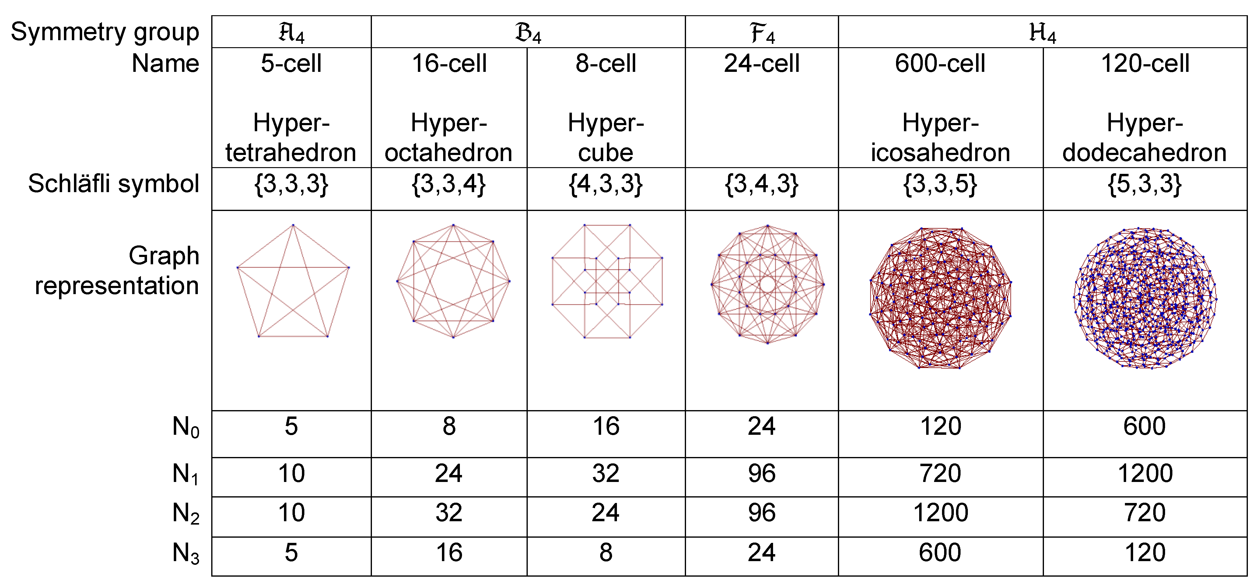
The six regular convex polytopes are summarized in Figure 3. Each of them is represented by a Schläfli symbol of the form $\{p,q,r\}$ in which p and q determine the Schläfli symbol $\{p,q\}$ for the 3-dimensional polyhedron that forms the boundary of the figure and r is the number of polyhedra meeting at one edge [17].

Polytopes with Schläfli symbols $\{p,q,r\}$ and $\{r,q,p\}$ are reciprocals of each other and belong to the same symmetry group. The six regular convex 4-polytopes therefore belong to only four symmetry groups. These are (i) the group ${\mathcal{A}}_4$ (isomorphic to the permutation group of 5 elements, $S_5$), populated by the 5-cell (hypertetrahedron); (ii) the group ${\mathcal{B}}_4$, populated by the mutually reciprocal 8-cell (hypercube) and 16-cell (hyperoctahedron); (iii) the group ${\mathcal{F}}_4$, populated by the 24-cell; and (iv) the group ${\mathcal{H}}_4$, populated by the mutually reciprocal 120-cell (hyperdodecahedron) and 600-cell (hypericosahedron).

Table 2. The four symmetry groups of the 4D regular polytopes. h denotes the total number of symmetry elements. The last column shows the number of elements in each class (in square parentheses), followed by a single symmetry element of the class, for a polytope in standard orientation. The symmetry elements are denoted $R_{{\mathbf{q}}_l,{\mathbf{q}}_r}$ for a proper rotation and ${\tilde{R}}_{{\mathbf{q}}_l,{\mathbf{q}}_r}$ for an improper rotation, see Equations 42 and 43. The quaternions $\{\mathbf{q}1,\mathbf{q}2\dots \mathbf{q}15\}$ are given explicitly in the last section.

Symmetry group	h	Symmetry operations
${\mathcal{A}}_4$	120	$\left[1\right]R_{\mathbf{q}1,\mathbf{q}1};\left[15\right]R_{\mathbf{q}3,\mathbf{q}3};\left[20\right]R_{\mathbf{q}8,\mathbf{q}8};\left[24\right]R_{\mathbf{q}11,\mathbf{q}12}$ $\left[10\right]{\tilde{R}}_{\mathbf{q}4,\mathbf{q}4};\left[30\right]{\tilde{R}}_{\mathbf{q}5,\mathbf{q}5};\left[20\right]{\tilde{R}}_{\mathbf{q}9,\mathbf{q}10}$
${\mathcal{B}}_4$	384	$\left[1\right]R_{\mathbf{q}1,\mathbf{q}1};\left[1\right]R_{\mathbf{q}1,-\mathbf{q}1};\left[6\right]R_{\mathbf{q}2,\mathbf{q}2};\left[12\right]R_{\mathbf{q}2,\mathbf{q}1};\left[12\right]R_{\mathbf{q}2,\mathbf{q}3};\left[24\right]R_{\mathbf{q}4,\mathbf{q}4};$ $\left[12\right]R_{\mathbf{q}6,\mathbf{q}6};\left[12\right]R_{\mathbf{q}6,-\mathbf{q}6};\left[32\right]R_{\mathbf{q}7,\mathbf{q}7};\left[32\right]R_{\mathbf{q}7,-\mathbf{q}7};\left[48\right]R_{\mathbf{q}6,\mathbf{q}4};$ $\left[4\right]{\tilde{R}}_{\mathbf{q}1,\mathbf{q}1};\left[4\right]{\tilde{R}}_{\mathbf{q}1,-\mathbf{q}1};\left[24\right]{\tilde{R}}_{\mathbf{q}2,\mathbf{q}1};\left[12\right]{\tilde{R}}_{\mathbf{q}4,\mathbf{q}4};\left[12\right]{\tilde{R}}_{\mathbf{q}4,-\mathbf{q}4};$ $\left[48\right]{\tilde{R}}_{\mathbf{q}6,\mathbf{q}4};\left[24\right]{\tilde{R}}_{\mathbf{q}6,\mathbf{q}6};\left[32\right]{\tilde{R}}_{\mathbf{q}7,\mathbf{q}7};\left[32\right]{\tilde{R}}_{\mathbf{q}7,-\mathbf{q}7}$
${\mathcal{F}}_4$	1152	$\left[1\right]R_{\mathbf{q}1,\mathbf{q}1};\left[1\right]R_{\mathbf{q}1,-\mathbf{q}1};\left[12\right]R_{\mathbf{q}2,\mathbf{q}1};\left[18\right]R_{\mathbf{q}2,-\mathbf{q}2};\left[96\right]R_{\mathbf{q}2,\mathbf{q}7};$ $\left[72\right]R_{\mathbf{q}4,\mathbf{q}4};\left[144\right]R_{\mathbf{q}6,-\mathbf{q}4};\left[36\right]R_{\mathbf{q}6,\mathbf{q}6};\left[36\right]R_{\mathbf{q}6,-\mathbf{q}6};\left[16\right]R_{\mathbf{q}7,\mathbf{q}1};$ $\left[16\right]R_{\mathbf{q}7,-\mathbf{q}1};\left[32\right]R_{\mathbf{q}7,\mathbf{q}7};\left[32\right]R_{\mathbf{q}7,-\mathbf{q}7};\left[32\right]R_{\mathbf{q}7,\mathbf{q}8};\left[32\right]R_{\mathbf{q}7,-\mathbf{q}8};$ $\left[12\right]{\tilde{R}}_{\mathbf{q}1,\mathbf{q}1};\left[72\right]{\tilde{R}}_{\mathbf{q}2,\mathbf{q}1};\left[12\right]{\tilde{R}}_{\mathbf{q}2,\mathbf{q}2};\left[96\right]{\tilde{R}}_{\mathbf{q}2,\mathbf{q}7};\left[12\right]{\tilde{R}}_{\mathbf{q}4,\mathbf{q}4};$ $\left[12\right]{\tilde{R}}_{\mathbf{q}4,-\mathbf{q}4};\left[72\right]{\tilde{R}}_{\mathbf{q}6,\mathbf{q}4};\left[96\right]{\tilde{R}}_{\mathbf{q}6,\mathbf{q}5};\left[96\right]{\tilde{R}}_{\mathbf{q}6,-\mathbf{q}5};\left[96\right]{\tilde{R}}_{\mathbf{q}7,\mathbf{q}1}$
${\mathcal{H}}_4$	14 400	$\left[1\right]R_{\mathbf{q}1,\mathbf{q}1};\left[1\right]R_{\mathbf{q}1,-\mathbf{q}1};\left[60\right]R_{\mathbf{q}1,\mathbf{q}3};\left[40\right]R_{\mathbf{q}1,\mathbf{q}13};\left[40\right]R_{\mathbf{q}1,-\mathbf{q}13};$ $\left[24\right]R_{\mathbf{q}1,\mathbf{q}14};\left[24\right]R_{\mathbf{q}1,-\mathbf{q}14};\left[24\right]R_{\mathbf{q}1,\mathbf{q}15};\left[24\right]R_{\mathbf{q}1,-\mathbf{q}15};\left[450\right]R_{\mathbf{q}3,\mathbf{q}3};$ $\left[1200\right]R_{\mathbf{q}3,\mathbf{q}13};\left[720\right]R_{\mathbf{q}3,\mathbf{q}14};\left[720\right]R_{\mathbf{q}3,\mathbf{q}15};\left[400\right]R_{\mathbf{q}13,\mathbf{q}13};\left[400\right]R_{\mathbf{q}13,-\mathbf{q}13};$ $\left[480\right]R_{\mathbf{q}13,\mathbf{q}14};\left[480\right]R_{\mathbf{q}13,-\mathbf{q}14};\left[480\right]R_{\mathbf{q}13,\mathbf{q}15};\left[480\right]R_{\mathbf{q}13,-\mathbf{q}15};\left[144\right]R_{\mathbf{q}14,\mathbf{q}14};$ $\left[144\right]R_{\mathbf{q}14,-\mathbf{q}14}\left[288\right]R_{\mathbf{q}14,\mathbf{q}15};\left[288\right]R_{\mathbf{q}14,-\mathbf{q}15};\left[144\right]R_{\mathbf{q}15,\mathbf{q}15};\left[144\right]R_{\mathbf{q}15,-\mathbf{q}15}$ $\left[60\right]{\tilde{R}}_{\mathbf{q}1,\mathbf{q}1};\left[60\right]{\tilde{R}}_{-\mathbf{q}1,\mathbf{q}1};\left[1800\right];{\tilde{R}}_{\mathbf{q}3,\mathbf{q}1};\left[1200\right]{\tilde{R}}_{\mathbf{q}13,\mathbf{q}1};\left[1200\right]{\tilde{R}}_{-\mathbf{q}13,\mathbf{q}1};$ $\left[720\right]{\tilde{R}}_{\mathbf{q}14,\mathbf{q}1};\left[720\right]{\tilde{R}}_{-\mathbf{q}14,\mathbf{q}1};\left[720\right]{\tilde{R}}_{\mathbf{q}15,\mathbf{q}1};\left[720\right]{\tilde{R}}_{-\mathbf{q}15,\mathbf{q}1};$
$\mathbf{q}1=\left(1,0,0,0\right);\mathbf{q}2=\left(0,0,0,1\right);\mathbf{q}3=\left(0,1,0,0\right);$
$\mathbf{q}4=\left(0,0,\frac{1}{\sqrt{2}},\frac{1}{\sqrt{2}}\right);\mathbf{q}5=\left(\frac{1}{\sqrt{2}},0,0,\frac{1}{\sqrt{2}}\right);\mathbf{q}6=\left(\frac{1}{\sqrt{2}},\frac{1}{\sqrt{2}},0,0\right);$
$\mathbf{q}7=\left(\frac{1}{2},\frac{1}{2},\frac{1}{2},\frac{1}{2}\right);\mathbf{q}8=\left(\frac{1}{2},-\frac{1}{2},-\frac{1}{2},-\frac{1}{2}\right);\mathbf{q}9=\left(\frac{1}{2\sqrt{2}},\frac{1}{2\sqrt{2}},\frac{1}{2\sqrt{2}},-\frac{\sqrt{5}}{2\sqrt{2}}\right);$
$\mathbf{q}10=\left(\frac{1}{2\sqrt{2}},\frac{1}{2\sqrt{2}},\frac{1}{2\sqrt{2}},\frac{\sqrt{5}}{2\sqrt{2}}\right);\mathbf{q}11=\left(\frac{\tau }{2},\frac{{\tau }^{-1}}{2},\frac{1}{2},0\right);\mathbf{q}12=\left(-\frac{{\tau }^{-1}}{2},-\frac{\tau }{2},\frac{1}{2},0\right);$
$\mathbf{q}13=\left(\frac{1}{2},\frac{{\tau }^{-1}}{2},\frac{\tau }{2},0\right);\mathbf{q}14=\left(\frac{\tau }{2},\frac{1}{2},\frac{{\tau }^{-1}}{2},0\right);\mathbf{q}15=\left(\frac{{\tau }^{-1}}{2},\frac{\tau }{2},\frac{1}{2},0\right)$

reports the four symmetry groups of the six regular polytopes and their symmetry elements, given in the quaternion form. The numbers of operations in each class are provided, together with one representative operation, using the notation $R_{{\mathbf{q}}_l,{\mathbf{q}}_r}$ for proper transformations and ${\tilde{R}}_{{\mathbf{q}}_l,{\mathbf{q}}_r}$ for improper transformations. In the case of the group ${\mathcal{H}}_4$, the symmetry classes and representative operations are given directly in quaternion form in Reference [23]. For the other groups, the information given in the literature [20,21,22] is not directly suitable for this type of analysis. In these cases, the quaternion form of the representative operations and the class structure were obtained by using the information provided in Reference [19] with the help of the symbolic software platform Mathematica [31].

4.6. Spherical Moments of the Regular 4-Polytopes

The spherical averaging properties of the regular 4-polytopes may be deduced by using Equation 20 together with the sets of symmetry operations (Table 2), and the characters of the 4D rotations, given in Equations 51 and 52.

As an example, consider the 5-cell, which has symmetry group ${\mathcal{A}}_4$. From Table 2, there are seven symmetry classes. The four classes of proper operations have $(1,15,20,24)$ elements respectively. The rotational angles $({\xi }_l,{\xi }_r)$ to be used in Equation 51 are obtained from Equation 7 and have the following values: $\left(\right(0,0)$, $(\pi ,\pi )$, $(2\pi /3,2\pi /3)$, $(2\pi /5,6\pi /5))$. The remaining three classes of improper operations have $(10,30,20)$ elements respectively. The rotational angles ${\xi }_{l,r}$ to be used in Equation 52 are obtained from Equations 7 and 37 and are as follows: $(2\pi ,\pi ,2\pi /3)$. The sum of characters for rank $\ell =1$ is therefore given by

$$\begin{array}{ccc}\hfill \sum _{\mathcal{C}}{h}_{\mathcal{C}}\left(T_d\right){\chi }_{\mathcal{C}}^{\left(1\right)}& =& {\chi }_D^{\left(1\right)}\left(0\right){\chi }_D^{\left(1\right)}\left(0\right)+15{\chi }_D^{\left(1\right)}\left(\pi \right){\chi }_D^{\left(1\right)}\left(\pi \right)+20{\chi }_D^{\left(1\right)}(2\pi /3){\chi }_D^{\left(1\right)}(2\pi /3)\hfill \\ & & +24{\chi }_D^{\left(1\right)}(2\pi /5){\chi }_D^{\left(1\right)}(6\pi /5)+10{\chi }_D^{\left(1\right)}\left(2\pi \right)+30{\chi }_D^{\left(1\right)}\left(\pi \right)+20{\chi }_D^{\left(1\right)}(2\pi /3)\hfill \\ & =& 0\hfill \end{array}$$

(53)

This proves that all first-rank spherical moments of a 5-cell are equal to zero:

$${\sigma }_{1m{m}^{\prime }}\left({\mathcal{A}}_4\right)=0$$

(54)

The spherical rank profiles of the other regular polytopes may be obtained in this way for any ℓ: Figure 4 summarizes the results up to rank $\ell =30$. As in the 3D case, even the 600-cell and 120-cell, which have the highest symmetry, fail to average out the rank-6 Wigner matrices.

This figure is slightly misleading since only integer ranks ℓ are shown. Since the groups ${\mathcal{B}}_4$, ${\mathcal{F}}_4$ and ${\mathcal{H}}_4$ possess an inversion operation, $R_{\mathbf{q}1,-\mathbf{q}1}$ with $\mathbf{q}1=(1,0,0,0)$, all spherical moments of half-integer rank vanish for these groups. The group ${\mathcal{A}}_4$, on the other hand, lacks the inversion, so the spherical moments of half-integer rank do not vanish in this case. The fact that ${\mathcal{A}}_4$ and ${\mathcal{B}}_4$ appear to have the same rank profiles in Figure 4 is therefore due to the omission of half-integer ranks. Most applications of orientational averaging only require integer ranks, in which case the properties shown in Figure 4 are appropriate.

There are 10 regular non-convex polytopes (star-polytopes) in four dimensions, which all fall in the group ${\mathcal{H}}_4$ [17]. Nine of them have the same vertices as the 600-cell, while one has the same vertices as the 120-cell. All have the same spherical moment characteristics as the 600-cell.

Under the reviewing of this paper, an anonymous referee pointed out that the pattern of empty and filled circles in Figure 4 may also be derived using the theory of spherical designs [18]. In general, 4D spherical harmonics of degree k generate a ${(k+1)}^2$-dimensional representation of the group $O\left(4\right)$ [18]. Such a representation is equivalent to the ${(2\ell +1)}^2$-dimensional representation constructed in Equation 48, with $k=2\ell$. A spherical t-design in 4 dimensions is defined as a subset of the hypersphere for which all the 4D spherical harmonics of degrees 1 to t average to 0 [18]. In other words, all the spherical moments of rank from 1 to $\ell =t/2$ vanish. In Reference [18] the largest values t of the spherical design have been derived to be 2 for the 5-cell, 3 for the 8-cell, 5 for the 24-cell, and 11 for the 600-cell, which correspond to $\ell =1,1,2,5$ in Figure 4.

The anonymous referee also pointed out that invariant theory may be used to prove that non-zero spherical moments in the ${\mathcal{H}}_4$ column in Figure 4 may appear at ℓ values corresponding to any sum of 6’s, 10’s and 15’s and for all $\ell \ge 30$.

5. Euler Angles

In order to facilitate exploitation of these results, we provide explicit tables of Euler angles derived from the vertices of the regular 4-polytopes. The $z-y-z$ convention for the Euler angles is used throughout. All Euler angle sets are derived from 4-polytopes in their standard orientations, as defined in

Table 3. The coordinates of the six convex regular 4-polytopes vertices in standard orientation, as reported in Reference [19]. The double round parentheses $\left(\right(\left)\right)$ indicate that all even permutations of the quartet are taken. The symbols $\tau$ and $\eta$ take the values $\tau =2\cos (\pi /5)=(\sqrt{5}+1)/2$ and $\eta =\sqrt{5}/4$. The 600 vertices of the hyperdodecahedron are obtained by multiplying the quaternion $(2^{-1/2},2^{-1/2},0,0)$ with all possible quaternion products of the 5 vertices of the hypertetrahedron S and the 120 vertices of the hypericosahedron I. All the polytopes are centred at the origin of the coordinate system, with the vertices lying on the hypersphere of radius 1.

Name	Vertex Coordinates
5-cell or hypertetrahedron	$S=\left\{\right(1,0,0,0),(-1/4,\eta ,\eta ,\eta ),(-1/4,-\eta ,-\eta ,\eta ),$
	$(-1/4,-\eta ,\eta ,-\eta ),(-1/4,\eta ,-\eta ,-\eta )\}$
16-cell or hyperoctahedron	$V=\left(\right(\pm 1,0,0,0\left)\right)$
8-cell or hypercube	$W=\left(\right(\pm 1/2,\pm 1/2,\pm 1/2,\pm 1/2\left)\right)$
24-cell	$T=V\cup W$
600-cell or hypericosahedron	$I=T\cup \frac{1}{2}\left((\pm \tau ,\pm 1,\pm {\tau }^{-1},0)\right)$
120-cell or hyperdodecahedron	$J=(2^{-1/2},2^{-1/2},0,0)\ast S\ast I$

. Ambiguities of the form given in Equation 41 were always resolved by choosing solutions with $\gamma =0$. All angles are reduced to the interval 0 to $2\pi$ by a modulo-$2\pi$ operation.

Different Euler angle sets with the same spherical averaging properties may be constructed by applying an equal but arbitrary 4D isometry to all the quaternions underlying the set.

The set of Euler angles corresponding to the 5 vertices of the 5-cell is provided in

Table 4. The set of Euler angles (in degrees) corresponding to the 5 vertices S of the 5-cell whose cartesian coordinates are given in Table 3.

$\alpha$	$\beta$	$\gamma$
0	0	0
69.0948	104.478	159.095
110.905	104.478	20.9052
249.095	104.478	339.095
290.905	104.478	200.905

. As shown in Figure 4, all first-rank spherical moments vanish for this set of Euler angles. Since the 5-cell lacks an inversion operation, the number of orientations is the same as the number of vertices in this case.

The sets of Euler angles corresponding to the 8 vertices of the 16-cell, and the 16 vertices of the 8-cell are provided in

Table 5. The set of Euler angles (in degrees) corresponding to the 8 vertices V of the 16-cell whose cartesian coordinates are given in Table 3. The 8 vertices are reduced to 4 sets of Euler angles because each quaternion pair $\{\mathbf{q},-\mathbf{q}\}$ corresponds to the same geometrical 3D rotation.

$\alpha$	$\beta$	$\gamma$
0	0	0
0	180	0
180	0	0
180	180	0

and

Table 6. The set of Euler angles (in degrees) corresponding to the 16 vertices W of the 8-cell whose cartesian coordinates are given in Table 3. The 16 vertices are reduced to 8 sets of Euler angles because each quaternion pair $\{\mathbf{q},-\mathbf{q}\}$ corresponds to the same geometrical 3D rotation.

$\alpha$	$\beta$	$\gamma$
0	90	90
0	90	270
90	90	0
90	90	180
180	90	90
180	90	270
270	90	0
270	90	180

. As shown in Figure 4, all first-rank spherical moments vanish for these sets of Euler angles. The symmetry groups of both polytopes include an inversion operation, so the number of distinguishable orientations is therefore one-half the number of the vertices. Clearly the four rotations specified in Table 5 comprise the most economical way to set all first-rank spherical moments to zero.

The set of 12 Euler angles corresponding to the 24 vertices of the 24-cell is provided in

Table 7. The set of Euler angles (in degrees) corresponding to the 24 vertices T of the 24-cell whose cartesian coordinates are given in Table 3. The 24 vertices are reduced to 12 sets of Euler angles because each quaternion pair $\{\mathbf{q},-\mathbf{q}\}$ corresponds to the same geometrical 3D rotation.

$\alpha$	$\beta$	$\gamma$	$\alpha$	$\beta$	$\gamma$
0	0	0	180	0	0
0	90	90	180	90	90
0	90	270	180	90	270
0	180	0	180	180	0
90	90	0	270	90	0
90	90	180	270	90	180

. As shown in Figure 4, all first and second-rank spherical moments vanish for this Euler angle set.

The sets of 60 and 300 Euler angles corresponding to the vertices of the 600-cell and the 120-cell are provided in

Table 8. The set of Euler angles (in degrees) corresponding to the 120 vertices I of the 600-cell whose cartesian coordinates are given in Table 3. The 120 vertices are reduced to 60 sets of Euler angles because each quaternion pair $\{\mathbf{q},-\mathbf{q}\}$ corresponds to the same geometrical 3D rotation.

$\alpha$	$\beta$	$\gamma$	$\alpha$	$\beta$	$\gamma$
0	0	0	180	0	0
0	90	90	180	90	90
0	90	270	180	90	270
0	180	0	180	180	0
20.9052	60	200.905	200.905	60	20.9052
20.9052	120	159.095	200.905	60	200.905
20.9052	60	20.9052	200.905	120	159.095
20.9052	120	339.095	200.905	120	339.095
58.2826	36	58.2826	238.283	36	58.2826
58.2826	36	238.283	238.283	36	238.283
58.2826	72	121.717	238.283	72	121.717
58.2826	72	301.717	238.283	72	301.717
58.2826	108	58.2826	238.283	108	58.2826
58.2826	108	238.283	238.283	108	238.283
58.2826	144	121.717	238.283	144	121.717
58.2826	144	301.717	238.283	144	301.717
90	90	0	270	90	0
90	90	180	270	90	180
121.717	36	121.717	301.717	36	121.717
121.717	36	301.717	301.717	36	301.717
121.717	72	58.2826	301.717	72	58.2826
121.717	72	238.283	301.717	72	238.283
121.717	108	121.717	301.717	108	121.717
121.717	108	301.717	301.717	108	301.717
121.717	144	58.2826	301.717	144	58.2826
121.717	144	238.283	301.717	144	238.283
159.095	60	159.095	339.095	60	159.095
159.095	60	339.095	339.095	60	339.095
159.095	120	20.9052	339.095	120	20.9052
159.095	120	200.905	339.095	120	200.905

and

Table 9. The set of Euler angles (in degrees) corresponding to the 600 vertices J of the 120-cell whose cartesian coordinates are given in Table 3. The 600 vertices are reduced to 300 sets of Euler angles because each quaternion pair $\{\mathbf{q},-\mathbf{q}\}$ corresponds to the same geometrical 3D rotation.

$\alpha$	$\beta$	$\gamma$	$\alpha$	$\beta$	$\gamma$	$\alpha$	$\beta$	$\gamma$	$\alpha$	$\beta$	$\gamma$
0	90	0	90	90	90	180	90	0	270	90	90
0	90	180	90	90	270	180	90	180	270	90	270
7.25597	49.1176	70.6909	90	180	0	187.256	49.1176	70.6909	270	180	0
7.25597	49.1176	250.691	95.6599	75.5225	137.470	187.256	49.1176	250.691	275.660	75.5225	137.470
7.25597	130.882	109.309	95.6599	75.5225	317.471	187.256	130.882	109.309	275.660	75.5225	317.471
7.25597	130.882	289.309	95.6599	104.478	42.5298	187.256	130.882	289.309	275.660	104.478	42.5298
14.5454	84.5204	131.110	95.6599	104.478	222.530	194.546	84.5204	131.110	275.660	104.478	222.530
14.5454	84.5204	311.110	98.3008	41.4096	98.3008	194.546	84.5204	311.110	278.301	41.4096	98.3008
14.5454	95.4796	48.8895	98.3008	41.4096	278.301	194.546	95.4796	48.8895	278.301	41.4096	278.301
14.5454	95.4796	228.890	98.3008	138.590	81.6992	194.546	95.4796	228.890	278.301	138.590	81.6992
20.9052	15.5225	20.9052	98.3008	138.590	261.699	200.905	15.5225	20.9052	278.301	138.590	261.699
20.9052	15.5225	200.905	105.450	69.7882	105.450	200.905	15.5225	200.905	285.450	69.7882	105.450
20.9052	44.4775	159.095	105.450	69.7882	285.450	200.905	44.4775	159.095	285.450	69.7882	285.450
20.9052	44.4775	339.095	105.450	110.212	74.5496	200.905	44.4775	339.095	285.450	110.212	74.5496
20.9052	60	110.905	105.450	110.212	254.550	200.905	60	110.905	285.450	110.212	254.550
20.9052	60	290.905	109.309	49.1176	172.744	200.905	60	290.905	289.309	49.1176	172.744
20.9052	75.5225	159.095	109.309	49.1176	352.7441	200.905	75.5225	159.095	289.309	49.1176	352.7441
20.9052	75.5225	339.095	109.309	130.882	7.25597	200.905	75.5225	339.095	289.309	130.882	7.25597
20.9052	104.478	20.9052	109.309	130.882	187.256	200.905	104.478	20.9052	289.309	130.882	187.256
20.9052	104.478	200.905	110.905	60	20.9052	200.905	104.478	200.905	290.905	60	20.9052
20.9052	120	69.0948	110.905	60	200.905	200.905	120	69.0948	290.905	60	200.905
20.9052	120	249.095	110.905	120	159.095	200.905	120	249.095	290.905	120	159.095
20.9052	135.522	20.9052	110.905	120	339.095	200.905	135.522	20.9052	290.905	120	339.095
20.9052	135.522	200.905	121.717	36	31.7175	200.905	135.522	200.905	301.717	36	31.7175
20.9052	164.478	159.095	121.717	36	211.717	200.905	164.478	159.095	301.717	36	211.717
20.9052	164.478	339.095	121.717	72	148.283	200.905	164.478	339.095	301.717	72	148.283
31.7175	36	121.717	121.717	72	328.283	211.717	36	121.717	301.717	72	328.283
31.7175	36	301.717	121.717	108	31.7175	211.717	36	301.717	301.717	108	31.7175
31.7175	72	58.2826	121.717	108	211.717	211.717	72	58.2826	301.717	108	211.717
31.7175	72	238.283	121.717	144	148.283	211.717	72	238.283	301.717	144	148.283
31.7175	108	121.717	121.717	144	328.283	211.717	108	121.717	301.717	144	328.283
31.7175	108	301.717	131.110	84.5204	14.5454	211.717	108	301.717	311.110	84.5204	14.5454
31.7175	144	58.2826	131.110	84.5204	194.546	211.717	144	58.2826	311.110	84.5204	194.546
31.7175	144	238.283	131.110	95.4796	165.455	211.717	144	238.283	311.110	95.4796	165.455
35.8898	25.2428	35.8898	131.110	95.4796	345.455	215.890	25.2428	35.8898	311.110	95.4796	345.455
35.8898	25.2428	215.890	137.470	75.5225	95.6599	215.890	25.2428	215.890	317.471	75.5225	95.6599
35.8898	154.757	144.110	137.470	75.5225	275.660	215.890	154.757	144.110	317.471	75.5225	275.660
35.8898	154.757	324.110	137.470	104.478	84.3401	215.890	154.757	324.110	317.471	104.478	84.3401
42.5298	75.5225	84.3401	137.470	104.478	264.340	222.530	75.5225	84.3401	317.471	104.478	264.340
42.5298	75.5225	264.340	144.110	25.2428	144.110	222.530	75.5225	264.340	324.110	25.2428	144.110
42.5298	104.478	95.6599	144.110	25.2428	324.110	222.530	104.478	95.6599	324.110	25.2428	324.110
42.5298	104.478	275.660	144.110	154.757	35.8898	222.530	104.478	275.660	324.110	154.757	35.8898
48.8895	84.5204	165.455	144.110	154.757	215.890	228.890	84.5204	165.455	324.110	154.757	215.890
48.8895	84.5204	345.455	148.283	36	58.2826	228.890	84.5204	345.455	328.283	36	58.2826
48.8895	95.4796	14.5454	148.283	36	238.283	228.890	95.4796	14.5454	328.283	36	238.283
48.8895	95.4796	194.546	148.283	72	121.717	228.890	95.4796	194.546	328.283	72	121.717
58.2826	36	148.283	148.283	72	301.717	238.283	36	148.283	328.283	72	301.717
58.2826	36	328.283	148.283	108	58.2826	238.283	36	328.283	328.283	108	58.2826
58.2826	72	31.7175	148.283	108	238.283	238.283	72	31.7175	328.283	108	238.283
58.2826	72	211.717	148.283	144	121.717	238.283	72	211.717	328.283	144	121.717
58.2826	108	148.283	148.283	144	301.717	238.283	108	148.283	328.283	144	301.717
58.2826	108	328.283	159.095	15.5225	159.095	238.283	108	328.283	339.095	15.5225	159.095
58.2826	144	31.7175	159.095	15.5225	339.095	238.283	144	31.7175	339.095	15.5225	339.095
58.2826	144	211.717	159.095	44.4775	20.9052	238.283	144	211.717	339.095	44.4775	20.9052
69.0948	60	159.095	159.095	44.4775	200.905	249.095	60	159.095	339.095	44.4775	200.905
69.0948	60	339.095	159.095	60	69.0948	249.095	60	339.095	339.095	60	69.0948
69.0948	120	20.9052	159.095	60	249.095	249.095	120	20.9052	339.095	60	249.095
69.0948	120	200.905	159.095	75.5225	20.9052	249.095	120	200.905	339.095	75.5225	20.9052
70.6909	49.1176	7.25597	159.095	75.5225	200.905	250.691	49.1176	7.25597	339.095	75.5225	200.905
70.6909	49.1176	187.256	159.095	104.478	159.095	250.691	49.1176	187.256	339.095	104.478	159.095
70.6909	130.882	172.744	159.095	104.478	339.095	250.691	130.882	172.744	339.095	104.478	339.095
70.6909	130.882	352.7441	159.095	120	110.905	250.691	130.882	352.7441	339.095	120	110.905
74.5496	69.7882	74.5496	159.095	120	290.905	254.550	69.7882	74.5496	339.095	120	290.905
74.5496	69.7882	254.550	159.095	135.522	159.095	254.550	69.7882	254.550	339.095	135.522	159.095
74.5496	110.212	105.450	159.095	135.522	339.095	254.550	110.212	105.450	339.095	135.522	339.095
74.5496	110.212	285.450	159.095	164.478	20.9052	254.550	110.212	285.450	339.095	164.478	20.9052
81.6992	41.4096	81.6992	159.095	164.478	200.905	261.699	41.4096	81.6992	339.095	164.478	200.905
81.6992	41.4096	261.699	165.455	84.5204	48.8895	261.699	41.4096	261.699	345.455	84.5204	48.8895
81.6992	138.590	98.3008	165.455	84.5204	228.890	261.699	138.590	98.3008	345.455	84.5204	228.890
81.6992	138.590	278.301	165.455	95.4796	131.110	261.699	138.590	278.301	345.455	95.4796	131.110
84.3401	75.5225	42.5298	165.455	95.4796	311.110	264.340	75.5225	42.5298	345.455	95.4796	311.110
84.3401	75.5225	222.530	172.744	49.1176	109.309	264.340	75.5225	222.530	352.7441	49.1176	109.309
84.3401	104.478	137.470	172.744	49.1176	289.309	264.340	104.478	137.470	352.7441	49.1176	289.309
84.3401	104.478	317.471	172.744	130.882	70.6909	264.340	104.478	317.471	352.7441	130.882	70.6909
90	0	0	172.744	130.882	250.691	270	0	0	352.7441	130.882	250.691

. Figure 4 shows that all spherical moments up to and including rank 5 vanish for these Euler angle sets. The most economical way of annihilating spherical ranks up to and including rank 5 is therefore the 60-angle set in Table 8. This rotation set was previously described in Reference [24], where it was presented without any supporting theory.

It is worth pointing out that the 3D rotations discussed above for the 24-cell and the 600-cell have more inutitive descriptions. The set of Euler angles obtained from the vertices of the 24-cell generates exactly the 12 rotational symmetries of the tetrahedron, compare Table 7 with the last column for the group $T_d$ in Table 1. Similarly the set of Euler angles obtained from the vertices of the 600-cell generates exactly the 60 rotational symmetries of the icosahedron, compare Table 8 with the last column for the group $I_h$ in Table 1. The 24 rotational symmetries of the cube ($O_h$ group) do not corresond to any regular 4-polytope. In fact they are not well distributed in the sense of particle repulsion over the hypersphere in 4D as the other polytopic cases. Regarding this last point, it has been rigorously proven that that some of the regular 4-polytopes (the 5-cell, the 16-cell and the 600-cell) minimize a full class of repulsive potentials over the 4D sphere [32].

6. Conclusions

We expect that these sets of rotations will be useful for the computation of orientational averages in a range of physical sciences, and in experimental procedures such as spherical tensor analysis in nuclear magnetic resonance [7,8,9]. In addition, we anticipate that where necessary, finer sampling of orientational space may be implemented by interpolating between the vertices of the polytopes, or by four-dimensional tiling and honeycomb schemes, such as those described by Coxeter [17].

Finally, we note that highly-symmetric four-dimensional figures have been found by using a computational procedure [33] which is closely related to the REPULSION algorithm on the surface of a sphere [3]. Such methods could be adapted to generate much larger sets of evenly spaced three-dimensional rotations than those described here.

References

- Mehring, M. High Resolution NMR in Solids, 2nd ed.; NMR-Basic Principles and Progress; Springer: Berlin, Germany, 1982; Volume 11. [Google Scholar]
- Levitt, M.H. Spin Dynamics. Basics of Nuclear Magnetic Resonance, 2nd ed.; Wiley: Chichester, UK, 2007. [Google Scholar]
- Bak, M.; Nielsen, N.C. REPULSION, A Novel Approach to Efficient Powder Averaging in Solid-State NMR. J. Magn. Reson. 1997, 125, 132–139. [Google Scholar] [CrossRef] [PubMed]
- Edén, M.; Levitt, M.H. Computation of Orientational Averages in Solid-State NMR by Gaussian Spherical Quadrature. J. Magn. Reson. 1998, 132, 220–239. [Google Scholar] [CrossRef] [PubMed]
- Edén, M. Computer simulations in solid-state NMR. III. Powder averaging. Concepts Magn. Reson. 2003, 18A, 24–55. [Google Scholar] [CrossRef]
- Stevensson, B.; Edén, M. Efficient orientational averaging by the extension of Lebedev grids via regularized octahedral symmetry expansion. J. Magn. Reson. 2006, 181, 162–176. [Google Scholar] [CrossRef] [PubMed]
- Suter, D.; Pearson, J.G. Experimental Classification of Multi-Spin Coherence under the Full Rotation Group. Chem. Phys. Lett. 1988, 144, 328–332. [Google Scholar] [CrossRef]
- Van Beek, J.D.; Carravetta, M.; Antonioli, G.C.; Levitt, M.H. Spherical tensor analysis of nuclear magnetic resonance signals. J. Chem. Phys. 2005, 122, 244510. [Google Scholar] [CrossRef] [PubMed]
- Pileio, G.; Levitt, M.H. Isotropic filtering using polyhedral phase cycles: Application to singlet state NMR. J. Magn. Reson. 2008, 191, 148–155. [Google Scholar] [CrossRef] [PubMed]
- Varshalovich, D.A.; Moskalev, A.N.; Khersonskii, V.K. Quantum theory of angular momentum; World Scientific Publishing: Teaneck, NJ, USA, 1988. [Google Scholar]
- Samoson, A.; Sun, B.Q.; Pines, A. New angles in motional averaging. In Pulsed Magnetic Resonance: NMR, ESR, and Optics, A recognition of E. L. Hahn; Bagguley, D.M.S., Ed.; Oxford Science Publications: Oxford, UK, 1992. [Google Scholar]
- Emsley, J.L.; Schmidt-Rohr, K.; Pines, A. Group theory and NMR dynamics. In NMR and More: In Honour of Anatole Abragam; Goldman, M., Por, M., Eds.; Les Editions de Physique: Paris, France, 1994. [Google Scholar]
- Lebedev, V.I. Quadratures on a Sphere. Zh. Vychisl. Mat. mat. Fiz. 1975, 15, 48. [Google Scholar] [CrossRef]
- Lebedev, V.I. Quadratures on a Sphere. Zh. Vychisl. Mat. mat. Fiz. 1976, 16, 293. [Google Scholar] [CrossRef]
- Lebedev, V.I.; Skorokhodov, A.L. Quadrature Formulas of Orders 41, 47 and 53 for the Sphere. Russian Acad. Sci. Dokl. Math. 1992, 45, 587. [Google Scholar]
- Weissenstein, E.W. Regular Polychoron. http://mathworld.wolfram.com/RegularPolychoron.html (accessed on 6 July 2010).
- Coxeter, H.S.M. Regular Polytopes; Methuen: London, UK, 1948. [Google Scholar]
- Delsarte, P.; Goethals, J.M.; Jacob, S.J. Spherical codes and designs. Geom. Dedicata 1977, 6, 363–388. [Google Scholar] [CrossRef]
- Du Val, P. Homographies, quaternions and rotations; Oxford University Press: Oxford, UK, 1964. [Google Scholar]
- Frobenius, F. Über die Charaktere der symmetrischen Gruppe. Sitzungberichte der Königlich Preussischen Akademie der Wissenschaften zu Berlin 1900, 516–534. [Google Scholar]
- Veysseyre, R.; Weigel, D.; Phan, T.; Effantin, J.M. Crystallography, geometry and physics in higher dimensions. II. Point symmetry of holohedries of the two hypercubic crystal systems in four-dimensional space. Acta Cryst. Sec. A 1984, 40, 331–337. [Google Scholar] [CrossRef]
- Kondo, T. The characters of the Weyl group of type F4. J. Fac. Sci. Univ. Tokyo Sect. I 1965, 11, 145–153. [Google Scholar]
- Grove, L.C. The characters of the hecatonicosahedroidal group. J. Reine Angew. Math. 1974, 265, 160–169. [Google Scholar]
- Levitt, M.H. An Orientational Sampling Scheme for Magnetic Resonance based on a Four-Dimensional Polytope. In Future Directions in Magnetic Resonance; Khetrapal, C.L., Ed.; Springer: Berlin, Germany, 2010. [Google Scholar]
- Armstrong, M.A. Groups and Symmetry; Sringer-Verlag: New York, NY, USA, 1988. [Google Scholar]
- Herstein, I.N. Topics in algebra, 2nd ed.; Xerox College Publishing: Lexington, KY, USA, 1975. [Google Scholar]
- Cotton, A. Chemical Applications of Group Theory, 3rd ed.; Wiley: New York, NY, USA, 1990. [Google Scholar]
- Hamermesh, M. Group theory and its application to physical problems; Addison-Wesley: London, UK, 1962. [Google Scholar]
- Altmann, S.L. Rotations, quaternions, and double groups; Oxford University Press: New York, NY, USA, 1986. [Google Scholar]
- Wigner, E.P. Group theory and its application to the quantum mechanics of atomic spectra; Academic Press: New York, NY, USA, 1971. [Google Scholar]
- Wolfram, S. Mathematica: A System for Doing Mathematics by Computer; Addison-Wesley: New York, NY, USA, 1991. [Google Scholar]
- Cohn, H.; Kumar, A. Universally optimal distribution of points on spheres. J. Amer. Math. Soc. 2007, 20, 99–148. [Google Scholar] [CrossRef]
- Altschuler, E.L.; Perez-Garrido, A.; Stong, R. A Novel Symmetric Four Dimensional Polytope Found Using Optimization Strategies Inspired by Thomson’s Problem of Charges on a Sphere. 2008; arXiv:physics/0601139v1. [Google Scholar]
Figure 1.
The 3D regular convex polyhedra organised according to their symmetry group. Here is the number of vertices, is the number of edges and is the number of faces constituting the solid.
Figure 2.
Spherical rank profiles for the regular convex 3D polyhedra. Open circles indicate that all spherical moments of integer rank ℓ are zero for the set of orientations corresponding to the vertices of the corresponding polyhedron. Closed circles indicate that there is at least one non-zero spherical moment of rank ℓ.
Figure 3.
A list of the 4D regular convex polytopes organized according to their symmetry group. Here is the number of vertices, is the number of edges, is the number of faces and is the number of three dimensional cells. The two dimensional graphs indicate the vertex connections.
Figure 4.
Spherical rank profiles of the regular convex 4-polytopes. Open circles indicate that all spherical moments of integer rank ℓ are zero for the set of orientations derived from the vertices of the corresponding polytope. Closed circles indicate that there is at least one non-zero spherical moment of rank ℓ.