Review of Kalman Filter Employment in the NAIRU Estimation

Abstract

The aim of the paper is to provide a recent overview of Kalman filter employment in the non-accelerating inflation rate of unemployment (NAIRU) estimation. The NAIRU plays a key part in an economic system. A certain unemployment rate which is consistent with a stable rate of inflation is one of the conditions for economic system stability. Since the NAIRU cannot be directly observed and measured, it is one of the most fitting problems for the Kalman filter application. The search for original, NAIRU focused and Kalman filter employment studies was performed in three scientific databases: Web of Science, Scopus, and ScienceDirect. A sample of 152 papers was narrowed down to 25 studies, which were described in greater detail regarding the focus, methods, model features, limitations, and other characteristics. A group of studies using a purely statistical approach of decomposing unemployment into a trend and cyclical component was identified. The next group uses the reduced-form approach which is sometimes combined with statistical decomposition. In such cases, the models are usually based on the backward-looking Phillips curve. Nevertheless, the forward-looking, New Keynesian or rarely hybrid New Keynesian variant can also be encountered.

1. Introduction

The Kalman filter is considered to be a theoretical basis for various recursive methods applied in stochastic (linear) dynamic systems. The algorithm is based on the idea that an unknown and unobservable state of the system can be estimated using certain measured data. The algorithm was named after Rudolf Emil Kalman, a Hungarian mathematician living in the USA, who presented it in 1960 in the text referred to below [1]. During the course of time, other authors derived other algorithms based on the principle of the Kalman filter. These algorithms are generally referred to as Kalman filters, and they can be conveniently applied in specific situations of solving practical problems in which, for example, some of the theoretical assumptions of the classical Kalman filter are not met.

The Kalman filter can be applied in varied domains of the prevailingly technical character, as for example in case of the localization of moving objects and navigation—the Kalman filter or Kalman filters in general are used in global navigation satellite systems (GPS, etc.), in radars, in the case of navigation and control of robots, in autopilots or autonomous vehicles, in computer vision for tracking objects in videos, in augmented and virtual reality, etc. Their application in the sphere of econometrics cannot be ignored, especially in the case of econometric models in which there is at least one variable which cannot be directly observed and measured.

One of the most fitting examples of such variables is the non-accelerating inflation rate of unemployment (NAIRU). The NAIRU is defined as the level of output and unemployment rate consistent with a stable rate of inflation. In other words, authors of the NAIRU concept claim that employment is an important criterion of policy, since it is at its natural level when neither inflationary nor deflationary pressure emanates from the labor market [2]. The labor market and unemployment levels have again become a frequently discussed topic in recent years, since world key economies are at or close to their peak in the business cycle. Unemployment rates below the NAIRU can be found in 2018 among the group of eight most advanced members economies (United States, Japan, Germany, United Kingdom) as well as among other European economies (Netherlands, Norway, Visegrad Group countries, Iceland, Malta) [3,4]. These rates are at or close to lowest values for the last decade which spurs the debate on labor market exhaustion, inflation pressure, and other related phenomena. These issues make the NAIRU estimation a current topic of discussion again and motivated us to create this review.

The article aims to provide an overview of NAIRU estimation studies and models with Kalman filter employment as a key part in the estimation process. The motivation of this focus was not only labor market issues in recent years but also the absence of an adequate recent review of the topic. Therefore, our goal is to fill this gap and contribute to authors who are performing the NAIRU estimation. For such authors, our review may provide a starting point inspiration as well as a summary of studies they should compare their own results to in the discussion section of their future works.

This article is structured as follows. In Section 2, we present Kalman filter employment in an unobserved variable estimation problem and our search strategy. Section 3 presents the results of the review of the 25 selected studies with a focus on study features such as aim, time series, model type, input and output variables, and their comparison. Finally, we summarize our conclusions in Section 4.

2. Methods

2.1. Kalman Filter

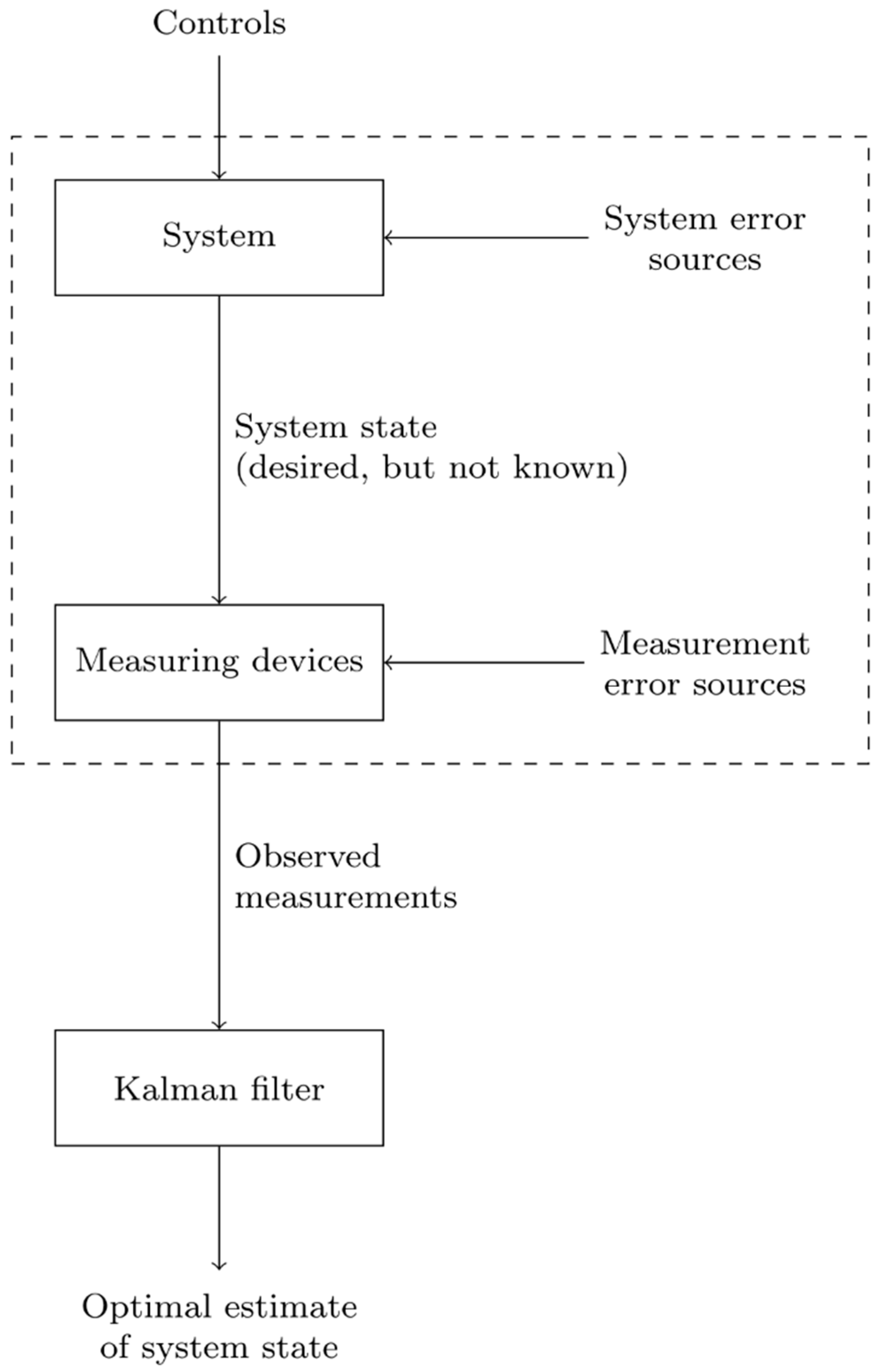
The Kalman filter is a tool which enables the estimation of the state of a stochastic linear dynamic system using measurements corrupted by noise. The estimate produced by the Kalman filter is statistically optimal in some sense (for example when considering the minimization of the mean square error; see [5] for details). The principle of the application of the filter is illustrated in Figure 1.

The Kalman filter works with all available information, i.e., all the available measurements, knowledge of the system model and the statistical description of its inaccuracies, noise and errors, and information about the initial conditions are used when the system state is being estimated.

Algorithm of the Kalman Filter

Let us consider a stochastic linear dynamic system in discrete time, which is represented by the following state-space model

$$\begin{array}{c}{\mathit{x}}_k={\mathbf{\Phi }}_{k-1}{\mathit{x}}_{k-1}+{\mathbf{\Gamma }}_{k-1}{\mathit{u}}_{k-1}+{\mathit{G}}_{k-1}{\mathit{w}}_{k-1},\end{array}$$

(1)

$$\begin{array}{c}{\mathit{z}}_k={\mathit{H}}_k{\mathit{x}}_k+{\mathit{D}}_k{\mathit{u}}_k+{\mathit{v}}_k.\end{array}$$

(2)

Equation (1), referred to as the state equation, describes the dynamics of the system. The vector ${\mathit{x}}_k\in {ℝ}^n$ is an (unknown) vector of the system state at the time $t_k$, the matrix ${\mathbf{\Phi }}_{k-1}\in {ℝ}^{n\times n}$ represents the system state transition between the time $t_{k-1}$ and $t_k$, the vector ${\mathit{u}}_k\in {ℝ}^r$ is a (known) vector of system control inputs, and the matrix ${\mathbf{\Gamma }}_k\in {ℝ}^{n\times r}$ is the input coupling matrix. Equation (2) is called the measurement equation. Vector ${\mathit{z}}_k\in {ℝ}^m$ is called the system output vector, the measurement vector or the observation vector; the matrix ${\mathit{H}}_k\in {ℝ}^{m\times n}$ describes the relation between the system state and the measurements; the matrix ${\mathit{D}}_k\in {ℝ}^{m\times r}$ is the input–output coupling matrix. Since a stochastic system is concerned, the vectors ${\mathit{x}}_k$ and ${\mathit{z}}_k$, $k=0,1,2,\dots$, can be considered as random variables, and their sequences $\left\{{\mathit{x}}_k\right\}$ and $\left\{{\mathit{z}}_k\right\}$ are then random (stochastic) processes.

$\left\{{\mathit{w}}_k\right\}$ and $\left\{{\mathit{v}}_k\right\}$ are random noise processes; these processes are assumed to be uncorrelated Gaussian processes with zero mean and covariance matrices ${\mathit{Q}}_k\in {ℝ}^{l\times l}$ resp. ${\mathit{R}}_k\in {ℝ}^{m\times m}$ at time $t_k$ (the processes have qualities of Gaussian white noise). Matrix ${\mathit{G}}_k\in {ℝ}^{n\times l}$ then describes the impact of the noise in the state equation of the model.

Furthermore, let us assume that ${\mathit{x}}_0$ is a random variable having a Gaussian (normal) distribution with known mean ${\mathit{x}}_0$ and known covariance matrix ${\mathit{P}}_0$. Moreover, suppose that ${\mathit{x}}_0$ and both the noises are always mutually uncorrelated. Then we can summarize that for all $t_k$,

$$E\langle {\mathit{w}}_k\rangle =\mathbf{0},$$

$$E\langle {\mathit{v}}_k\rangle =\mathbf{0},$$

$$E\langle {\mathit{w}}_{k_1}{\mathit{w}}_{k_2}^T\rangle ={\mathit{Q}}_{k_1}\Delta \left(k_2-k_1\right),$$

$$E\langle {\mathit{v}}_{k_1}{\mathit{v}}_{k_2}^T\rangle ={\mathit{R}}_{k_1}\Delta \left(k_2-k_1\right),$$

$$E\langle {\mathit{w}}_{k_1}{\mathit{v}}_{k_2}^T\rangle =\mathbf{0},$$

$$E\langle {\mathit{x}}_0{\mathit{w}}_k^T\rangle =\mathbf{0},$$

$$E\langle {\mathit{x}}_0{\mathit{v}}_k^T\rangle =\mathbf{0},$$

where the symbol $\Delta$ refers to the Kronecker delta,

$$\Delta \left(k\right)=\{\begin{array}{l}1,k=0,\\ 0,k\ne 0.\end{array}$$

The aim of the Kalman filter is to produce an estimate of the state vector ${\mathit{x}}_k$ at time $t_k$, symbolized as ${\widehat{\mathit{x}}}_k$, so that this estimate is optimal (for example with respect to minimizing the mean square error).

The algorithm of the Kalman filter is recursive; the calculation at time $t_k$ consists of two main steps. Firstly, the a priori estimate ${\widehat{\mathit{x}}}_{k(-)}$ at time $t_k$ is computed through substituting the a posteriori estimate from time $t_{k-1}$ into the deterministic part of the state equation of the model; this step is called the prediction step. Then, this estimate is improved by using the measurement carried out at time $t_k$, which results in obtaining the a posteriori estimate ${\widehat{\mathit{x}}}_{k(+)}$ at time $t_k$; this is the correction step.

The following relation can be written to specify the a priori estimate of the state vector ${\widehat{\mathit{x}}}_{k(-)}$ at time $t_k$; the uncertainty of this estimate is expressed by the a priori error covariance matrix ${\mathit{P}}_{k(-)}$

$${\widehat{\mathit{x}}}_{k(-)}={\mathbf{\Phi }}_{k-1}{\widehat{\mathit{x}}}_{k-1(+)}+{\mathbf{\Gamma }}_{k-1}{\mathit{u}}_{k-1},$$

$${\mathit{P}}_{k(-)}={\mathbf{\Phi }}_{k-1}{\mathit{P}}_{k-1(+)}{\mathbf{\Phi }}_{k-1}^T+{\mathit{G}}_{k-1}{\mathit{Q}}_{k-1}{\mathit{G}}_{k-1}^T.$$

Then, after obtaining the measurement ${\mathit{z}}_k$, combining the a priori estimate and the difference between the actual value and the predicted value of the measurement weighted by the matrix ${\mathit{K}}_k$, we come to the a posteriori estimate of the state vector ${\widehat{\mathit{x}}}_{k(+)}$; its uncertainty is expressed by the a posteriori error covariance matrix ${\mathit{P}}_{k(+)}$

$${\widehat{\mathit{x}}}_{k(+)}={\widehat{\mathit{x}}}_{k(-)}+{\mathit{K}}_k\left[{\mathit{z}}_k-{\mathit{D}}_k{\mathit{u}}_k-{\mathit{H}}_k{\widehat{\mathit{x}}}_{k(-)}\right],$$

$${\mathit{P}}_{k(+)}={\mathit{P}}_{k(-)}-{\mathit{K}}_k{\mathit{H}}_k{\mathit{P}}_{k(-)},$$

$${\mathit{K}}_k={\mathit{P}}_{k(-)}{\mathit{H}}_k^T{\left[{\mathit{H}}_k{\mathit{P}}_{k(-)}{\mathit{H}}_k^T+{\mathit{R}}_k\right]}^{-1}.$$

A detailed derivation of the given equations of the Kalman filter can be found for example in [6]; more detailed presentations of the algorithm, its features and its theoretical assumptions can be found for example in [5,6,7]; practical aspects of the implementation of the filter are discussed for example in [7].

2.2. Search Strategy, Eligibility Criteria, Data Extraction, and Article Evaluation

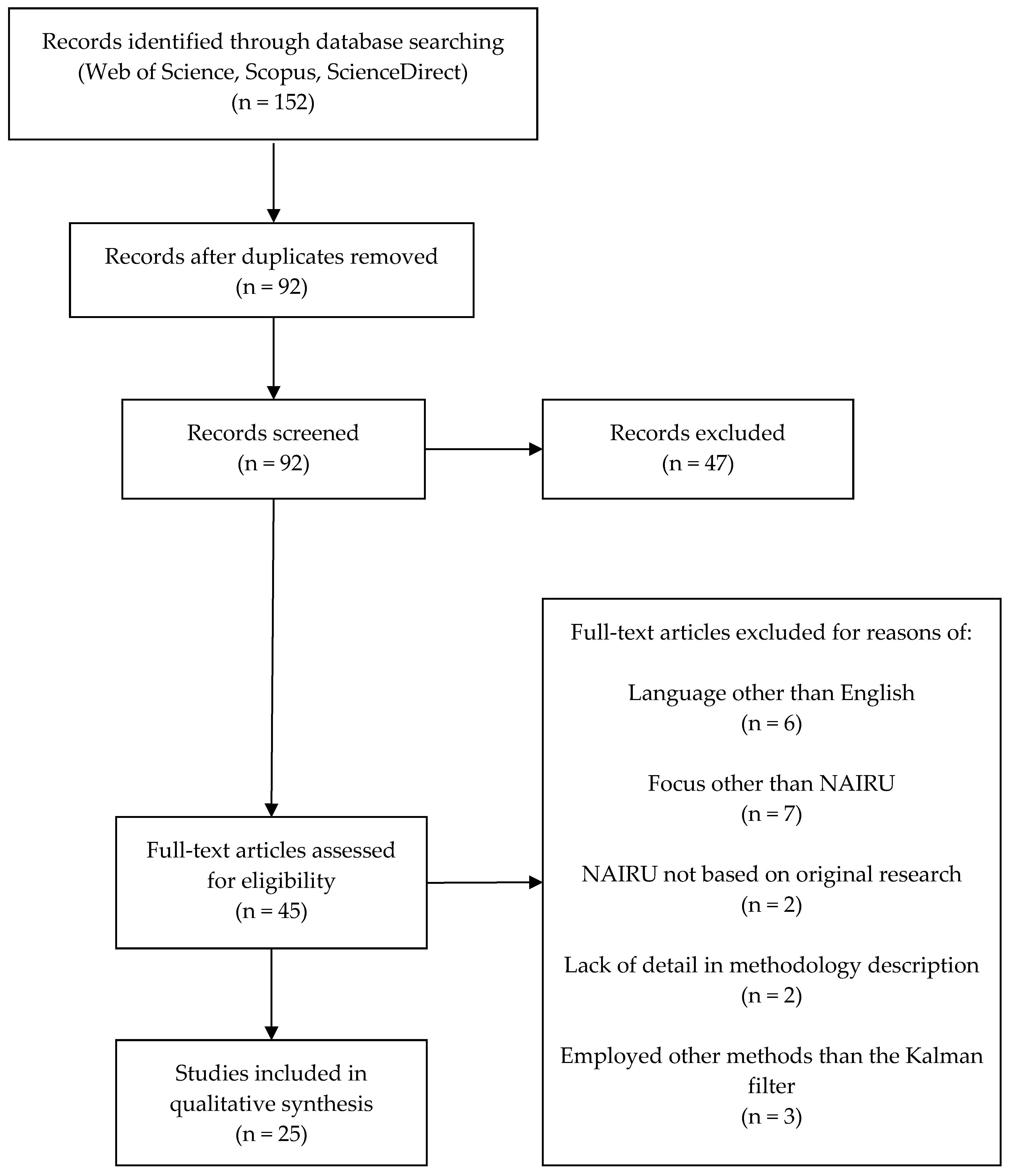
A systematic literature search was preceded by a short pre-search phase performed in the EBSCO Discovery Service. Although the search in the EBSCO Discovery Service can find papers in other sites such as ScienceDirect and Scopus, it was used for the pre-search only. It is usually counted among and compared to more general or broad academic search tools, see, e.g., [8,9], than among strictly science-focused databases. The systematic literature search was conducted by two researchers during February 2019. The search covered three research databases: Web of Science, Scopus, and ScienceDirect. Both keywords were combined in a “Title, abstract, keywords” search query: “Kalman filter” AND NAIRU. Searches resulted in 34 identified records in the Web of Science, 37 in the Scopus, and 81 in the ScienceDirect.

Eliminating duplicate records reduced the sample to 92 records, which was followed by a screening phase. For each record, three scientists extracted the author, the title of the study, keywords, abstract and type of record. Some of the papers proved to be false positives. While they contained the appropriate keywords, the rest of them or a study description in the abstract suggested otherwise. The content was not relevant to the topic due to a focus on other topics such as the mining industry, exchange rates and other areas which are affected by the economic cycle. The screening phase also removed document types such as book chapters, short communications, short papers, and proceedings papers. It was decided to exclude proceedings papers from the search since screening showed that sources of such papers were conferences such as the International Business Information Management Association (IBIMA). In particular, this type of source was present in Beall’s list, and in some universities, these are strongly recommended to be avoided due to an overall lack of quality in the peer review process. In this phase, the sample was reduced to 45 full-length journal articles.

In the last phase of a record assessment, articles were assessed accordingly eligibility criteria. In order to be eligible for analysis, the papers had to meet the following criteria:

• Published after 2005. We chose a fifteen-year timespan, even though most of the reviews focus on a ten-year timespan, to avoid obsolete studies. However, theoretical foundations for the target problem were published even before the year 2000, and observed paradigms were not fundamentally challenged since then. Secondly, data series of macroeconomics related statistics are available for much longer compared to, e.g., business-related time series. This advantage is due to the overall importance of fundamental macroeconomic identities data.
• Written in the English language. The criterion was chosen to maximize the readability of the described studies.
• Presenting original research. The criterion was applied to prevent the inclusion of papers which were based on NAIRU values presented in other papers. In such cases, NAIRU values usually served only as, e.g., inputs of a different model or economy development indicator.
• Describing a methodology related to an unobservable variable estimation. Methodology requirement was adopted since some studies stated very briefly that there was data treatment, yet there were no details on methods and settings, or other details.
• Focused on the NAIRU. An article had to be focused on the NAIRU estimation for individual economies, on a new method on how to obtain the estimates or to estimate and test the dependence of the NAIRU on several factors (such as unemployment versus structural factors, institutional factors, etc.). The NAIRU was in some articles included only to demonstrate an economic environment change, but a study focus was on the New economy paradigm, and the Kalman filter was employed for other purposes.
• Employing the Kalman filter. The last criterion deals with the fact that there are also other ways how to perform the NAIRU estimation by employing, e.g., the Hodrick–Prescott filter.

The eligibility criteria reduced the sample to a final count of 25 studies. The full paper acquisition was followed by individual article processing. See the scheme in Figure 2 for a search process overview.

3. Results and Discussion

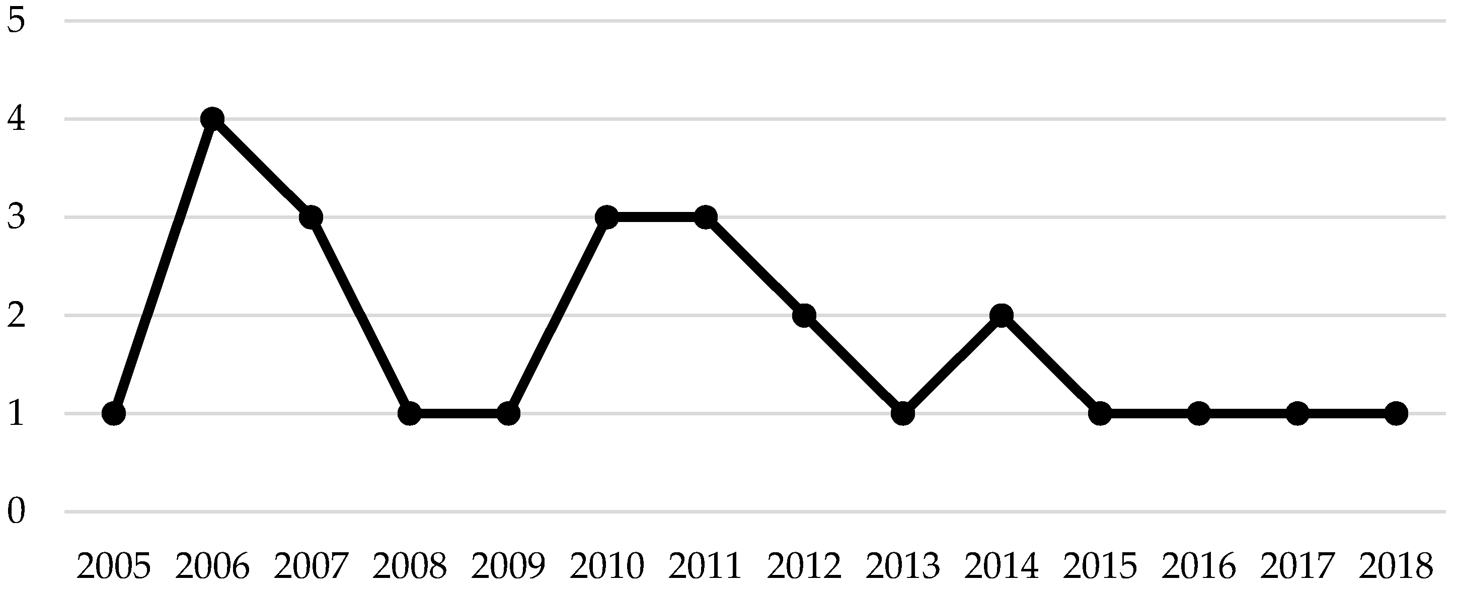
The review sample consisted of 25 studies, which were unevenly distributed in time; see Figure 3. The number of papers published per year with a focus on Kalman filter employment in the NAIRU estimation varies in time in a nonlinear way. The highest count can be found in the years of an economic upturn before the last global economic crisis. However, the count decreases in the same part of a business cycle in 2018.

3.1. Overview of Analysed Studies

Table 1. Overview of the studies.

	Authors	Publication Year	Aim	Country	Time Series Data
[10]	Aguiar, A.; Martins, M.M.F.	2005	Testing possible non-linearity in a NAIRU model, estimating the NAIRU	Euro area countries (aggregated)	Q, 1970:Q1–2002:Q3
[11]	Andrei, A.M.	2014	Estimating the NAIRU and potential output	Romania	Q, 2001:Q1–2014:Q2
[12]	Andrei, A.M.; Galupa, A.; Georgescu, I.	2017	Estimating potential output	Romania	Q, 2000–2013:Q2
[13]	Basistha, A.; Nelson, C.R.	2007	Estimating the output gap	USA	Q, 1960:Q1–2003:Q1
[14]	Batini, N.; Greenslade, J.V.	2006	Estimating the short-run NAIRU and discussing the usefulness of the NAIRU concept	UK	Q, 1973:Q1–2001:Q4
[15]	Berger, T.	2011	Estimating the NRU, potential output and the core inflation rate	Euro area countries (aggregated)	Q, 1970–2005
[16]	Berger, T.; Everaert, G.	2010	Analyzing effects of labor taxes on unemployment	OECD countries (16 countries grouped into three groups: AT, DK, FI, SE; BE, FR, DE, IT, NL, PT, ES, GR; JP, IE, US, GB)	A, 1970–2005
[17]	Botric, V.	2012	Estimating the NAIRU	Croatia	Q, 2000:Q1–2011:Q2
[18]	Claar, V.V.	2006	Estimating the NRU and evaluating its inflation-forecasting power relative to the NAIRU	USA	A, 1947–1998
[19]	Constantinescu, M.; Nguyen, A.D.M.	2018	Estimating potential output	Lithuania	Q, 1998:Q1–2016:Q3
[20]	Domenech, R.; Gomez, V.	2006	Estimating the NAIRU, the core inflation rate and the investment rate trend	USA	Q, 1947:Q1–2003:Q1
[21]	Elkayam D.; Ilek A.	2016	Estimating the NAIRU	Israel	Q, 1992:Q1–2013:Q4
[22]	Fitzenberger, B.; Franz, W.; Bode, O.	2008	Estimating the NAIRU	Germany	Q, 1976:Q2–1990:Q2 (West Germany), 1990:Q3–2006:Q4 (unified Germany)
[23]	Heyer, E.; Reynes, F.; Sterdyniak, H.	2007	Comparing two approaches for estimating the NAIRU	France, USA	Q, 1970–2003
[24]	Leu, S. C.-Y.; Sheen, J.	2011	Estimating the NAIRU, potential output, the neutral real interest rate and the subjective discount factor	Australia	Q, 1984:Q1–2006:Q4
[25]	Logeay, C.; Tober, S.	2006	Estimating the NAIRU and analyzing the hysteresis effect	Euro area countries (12 countries: DE, FR, IT, ES, NL, AT, PT, FI, IE, BE, LU, GR)	Q, 1970–2002
[26]	Marjanovic, G.; Maksimovic, L.; Stanisic, N.	2015	Estimating the NAIRU and analyzing the hysteresis effect for countries in transition	Countries in transition (Eight countries: PL, HU, CZ, SK, SI, BG, RO, HR)	Q, 2000–2012
[27]	Melihovs, A.; Zasova, A.	2009	Estimating the NAIRU and the NAIRCU	Latvia	Q, 1996:Q3–2008:Q4
[28]	Napolitano O.; Montagnoli A.	2010	Estimating the NAIRU and analyzing the impact of monetary policy on the labor market	France, Germany, Italy	Q, 1972:Q1–2007:Q1
[29]	Planas, C.; Roeger, W.; Rossi, A.	2007	Analyzing effects of labor taxes on unemployment, estimating the NAIRU	Euro area countries (aggregated 12 countries: DE, FR, IT, ES, NL, AT, PT, FI, IE, BE, LU, GR)	A, 1970–2004
[30]	Rodriguez G.	2010	Estimating the NAIRU, the output gap and the core inflation	Peru	Q, 1979:Q1–2007:Q4
[31]	Rodriguez, A.; Ruiz, E.	2012	Calculating uncertainty of the NAIRU, the output gap, the long-run investment rate and the core inflation estimates	USA	Q, 1948:Q1–2003:Q1
[32]	Rusticelli E.	2014	Estimating the NAIRU considering the hysteresis effect	OECD countries (11 countries: CA, FR, DE, GR, IE, IT, JP, PT, ES, GB, US)	Q, 1987:Q1–2012:Q4 (different starting points for different countries)
[33]	Shaheen F.; Haider A.; Javed S. A.	2011	Estimating the NAIRU	Pakistan	A, 1973/74–2007/08
[34]	Valadkhani A.; Araee S.M.M.	2013	Estimating the NAIRU	Iran	A, 1959–2008

Abbreviations: NAIRU— non-accelerating inflation rate of unemployment, NRU—natural rate of unemployment, NAIRCU—non-accelerating inflation rate of capacity utilization; Q—quarterly data, A—annual data; country codes ISO 3166-1 alpha-2.

provides an overview of the 25 analyzed studies. For each study, the following details are stated: authors, publication year, aim, country/countries, time period studied.

The aim of the studies is the estimation of the NAIRU and other unobservable economic variables. There are some studies which also examine the factors influencing the NAIRU.

Most of the studies are focused on European countries, and especially on euro area countries. Some authors do distinguish countries but for the euro area countries, it is also common for authors to base their study on the aggregated data of all countries. Outside Europe, there are studies that are focused mostly on developed economies such as the United States, Canada, Japan, Israel, and Australia. It is rare to find such a study for emerging markets or less developed countries. However, a few of the studies were focused on Peru, Pakistan, and Iran. Most of the studies use data obtained on a quarterly basis. Only five studies use annual time series. The monitored period varies significantly from 11.5 to 56 years.

3.2. Description and Discussion of Approaches and Models Used in the Analysed Studies

The NAIRU is in its nature an unobservable phenomenon, and the Kalman filter can serve as one of the means for its estimation. There are several ways in which the Kalman filter can be employed to solve this problem.

The most straightforward approach to the NAIRU estimation is a purely statistical one. It is based on an unemployment decomposition into a trend component and cyclical component. The trend component is then corresponding to the NAIRU. This approach is based on the idea that unemployment fluctuates around the NAIRU in the long run. The fluctuation is a result of self-balancing forces in an economy. At the same time, it represents the decomposition of unemployment into structural, frictional and cyclical, where the first two components are considered as the NAIRU.

Unemployment decomposition can be expressed by a simple equation

$$\begin{array}{c}{u}_t=u_t^{*}+u_t^c,\end{array}$$

(3)

where $u_t$ is the real total unemployment, $u_t^{*}$ is the NAIRU, and $u_t^c$ is the cyclical component of unemployment. There are different statistical techniques and tools for time series decomposition into a trend and cyclical components. The Kalman filter is one of these tools.

The reduced-form approach is the most commonly used approach for the NAIRU estimation. This approach is based on the Phillips curve. It is founded on the relationship between unemployment and inflation, thus directly following the definition of the NAIRU as an unemployment rate corresponding to stable inflation.

This approach is more flexible compared to the first one. It allows using inflation information and the impact of various other factors, thus improving economic interpretation of results. The unobservability of the NAIRU and other variables can be appropriately addressed using the Kalman filter.

The starting point is the Phillips curve equation, e.g.,

$$\begin{array}{c}{\pi }_t=\alpha \left(L\right){\pi }_{t-1}+\beta \left(L\right)\left(u_t-u_t^{*}\right)+\gamma \left(L\right){\mathit{z}}_t+{\epsilon }_t^{pc},\end{array}$$

(4)

where ${\pi }_t$ stands for inflation, $u_t-u_t^{*}$ for the unemployment gap and ${\mathit{z}}_t$ for the vector of supply shocks. $\alpha \left(L\right)$, $\beta \left(L\right)$, $\gamma \left(L\right)$ are lag operators. Lagged inflation $\alpha \left(L\right){\pi }_{t-1}$ represents inflation expectations, assuming ${\alpha }_0+{\alpha }_1+\cdots +{\alpha }_q=1$. It is common to express the equation in terms of the first difference of inflation and also variables are often logarithmized. Equation (4) follows Gordon’s triangle model which is consisted of three components: inertia (${\pi }_{t-1}$), demand ($u_t-u_t^{*}$), supply (${\mathit{z}}_t$). The distinction between the triangle model and the original Phillips curve is that the former measures changes in prices, not changes in wage rates [2].

The equation itself differs from one author to another. In particular, there is a difference in supply shocks selection or the number of lags. For example, the most common supply shocks are the change in real import prices and the change in real oil prices [14,27,32]. The choice of a particular supply shock inclusion depends on a surveyed country, i.e., on the results of testing the statistical significance of the corresponding model coefficients. The shocks should be uncorrelated, although [15] allows correlation. Some authors do not include supply shocks or inflation expectations in the equation at all [11,12,19]. On the other hand, other authors add dummy variables to identify the season (quarter) [22] or a structural break. Such break represents, e.g., situation before and after the German reunification in 1990 [22,25] or the last economic crisis [17]. See

Table 2. Overview of the models used in the studies.

	Model	Estimated Output Variables	Additional Input Variables
[10]	Backward-looking PC; OL	NAIRU	Deviation of imported inflation from domestic inflation in the previous quarter
[11]	Backward-looking PC	NAIRU *	-	* NAIRU estimates are used for calculating potential output
[12]	Backward-looking PC	NAIRU *	-	* NAIRU is estimated in two steps; potential output is then estimated using the NAIRU estimates
[13]	NKPC; OL; decomposition of unemployment, output and inflation into gap and non-gap component, which are not identical to cycle and trend	NRU *, output gap	-	* NRU is used as a synonym for NAIRU
[14]	Backward-looking PC *	NAIRU **	Change in real import prices, change in real oil prices	* 2 models ** The longer-run NAIRU is estimated using the Kalman filter and then the short-run NAIRU is derived from these estimates
[15]	NKPC; OL; trend-cycle decomposition of unemployment, output and inflation	NRU *, potential output, core inflation rate	Dummy for structural break	* NRU is used as a synonym for NAIRU
[16]	Trend-cycle decomposition of unemployment; decomposition of the trend into observable (a labor tax effect) and unobservable component	NAIRU, cyclical unemployment *	Labor taxes	* The main aim of the study is estimating unknown model parameters and testing their significance
[17]	Backward-looking PC	NAIRU	Change in real oil prices; dummy for crisis effect
[18]	Trend-cycle decomposition of unemployment	NRU *	-	* NRU estimates are used for inflation forecasting; NRU is distinguished from NAIRU
[19]	Backward-looking PC; OL; trend-cycle decomposition of unemployment, output and inflation	NAIRU, potential output	-
[20]	Forward-looking PC; OL; trend-cycle decomposition of output, investment equation	NAIRU, potential output, core inflation rate, investment rate trend	-
[21]	Forward-looking PC	NAIRU	Change in real import prices
[22]	Backward-looking PC; OL *	NAIRU	Relative inflation rate of imported raw materials, change rate of price wedge, rate of change of labor productivity minus trend rate of change; dummy for structural break; quarter dummies	* 6 models
[23]	Backward-looking PC *	NAIRU	Change in real import prices	* 2 models (differing from each other by the inclusion of additional exogenous variables in the NAIRU equation)
[24]	Hybrid NKPC; OL; New Keynesian dynamic IS equation; trend-cycle decomposition of unemployment, output and the real interest rate	NAIRU, potential output, neutral real interest rate, subjective discount factor	Dummy for the exogenous effect of the introduction of the Goods and Services Tax in Australia in 2000
[25]	Backward-looking PC	NAIRU	Change in real oil prices, change in labor productivity growth; dummy for structural break (Germany)
[26]	Trend-cycle decomposition of unemployment	NAIRU	-
[27]	Backward-looking PC; trend-cycle decomposition of unemployment	NAIRU *	Change in real oil prices, change in real import prices	* NAIRCU is estimated using different model
[28]	Trend-cycle decomposition of unemployment	NAIRU	-
[29]	Trend-cycle decomposition of unemployment; decomposition of the trend into observable (a labor tax effect) and unobservable component	NAIRU	Labor taxes
[30]	NKPC; OL; trend-cycle decomposition of output, investment equation	NAIRU, potential output, core inflation rate	-
[31]	Forward-looking PC; OL; trend-cycle decomposition of output; investment equation	NAIRU, potential output, core inflation, long-run investment rate	-
[32]	Backward-looking PC; trend-cycle decomposition of unemployment *	NAIRU	Change in real import price inflation weighted by import penetration, change in real oil price inflation weighted by oil intensity of production	* The change in the lagged long-term unemployment rate is included in the NAIRU equation to capture the hysteresis effect
[33]	Trend-cycle decomposition of unemployment; backward-looking PC *	NAIRU	Change in real oil prices; dummy for changes in inflation	* NAIRU is estimated in two steps (1. step: trend-cycle decomposition, 2. step: estimation using PC)
[34]	Backward-looking PC *	NAIRU	Aggregate import price index	* 2 models (the second model is augmented by the output gap calculated using the HP filter)

Abbreviations: PC—Phillips curve, NKPC—New Keynesian Phillips curve, OL—Okun’s law, NAIRU— non-accelerating inflation rate of unemployment, NRU—natural rate of unemployment, NAIRCU—non-accelerating inflation rate of capacity utilization.

for more details. The study [10] also mentions an issue of a possible nonlinearity of the Phillips curve.

It is necessary to further specify the evolution of the NAIRU over time to complement the model—the NAIRU is understood as a stochastic process. The simplest option is to assume the NAIRU to be constant over time. This assumption may be applicable in situations where a level of unemployment fluctuates around a certain mean without a noticeable upward or downward trend. However, for most countries, this is not the case. Therefore, it is appropriate to work with a time-varying NAIRU.

The NAIRU is most often described as a random walk.

$$\begin{array}{c}{u}_t^{*}=u_{t-1}^{*}+{\epsilon }_t^n.\end{array}$$

(5)

This model of the NAIRU evolution is generally considered appropriate for the United States [18,20,31]. On the other hand, some authors [15,20] prefer a random walk with drift which is more suitable for European countries. The NAIRU can be also expressed in the form of an autoregressive (AR) process; for example [11,12,16] use the AR(2) process to represent the hysteresis effect. The study [32] adds a long-term unemployment variable in order to reflect hysteresis; [25] represents hysteresis by the lagged unemployment rate. The choice of a model depends on the conditions of a studied country and is based on a statistical analysis of unemployment time series. The analysis employs unit root tests, especially an augmented Dickey–Fuller (ADF) test.

Equation (4) represents the measurement equation and Equation (5) represents the state equation of the basic model for the NAIRU estimation. Both equations are transformed into the state-space form and then the Kalman filter can be applied (see Section 3.3. for more details). Nevertheless, the model can be further extended by various means. The most common way is including the NAIRU-potential output relation. The potential output is another unobservable theoretical economic variable. This relation, i.e., the link between the output gap and the unemployment gap, can be expressed by the Okun’s law equation

$$\begin{array}{c}{y}_t-y_t^{*}=\delta \left(L\right)\left(u_t-u_t^{*}\right)+{\epsilon }_t^{ol},\end{array}$$

(6)

where $y_t$ is real output and $y_t^{*}$ is potential output of an economy.

Furthermore, this way comprises adding a description of potential output evolution, for example in the form of a random walk with drift process

$$\begin{array}{c}{y}_t^{*}=\mu +y_{t-1}^{*}+{\epsilon }_t^p\end{array}$$

(7)

and specifying a process of the unemployment gap evolution (evolution of cyclical fluctuations in unemployment)

$$\begin{array}{c}{u}_t-u_t^{*}=\varphi \left(L\right)\left(u_t-u_t^{*}\right)+{\epsilon }_t^g.\end{array}$$

(8)

It is assumed for all the equations above that $\left\{{\epsilon }_t^x\right\}$ are uncorrelated Gaussian processes with zero means and constant variances ${\sigma }_x^2$.

Equations (4)–(8) form the model created by Apel and Jansson [35,36], which became a starting point for most authors such as [10,22].

Models combining this described reduced-form approach with a statistical decomposition of unemployment into trend and cycle can also be found.

Another possibility is to start from the classic wage Phillips curve, although the price Phillips curve is preferred in practice over the wage curve. Some authors employ different models based on the forward-looking Phillips curve [20,21,31] or the New Keynesian Phillips curve [13,15,24,30], which are complemented by equations describing the relationship with unemployment, output or other variables. The Kalman filter can be appropriately used in such models to allow addressing the problem of unobservability of expected future inflation.

Doménech and Gómez [20] include even more unobservable variables—the core inflation and the investment rate trend. Such a model consists of the equation of GDP decomposition into trend and cycle, the forward-looking Phillips curve equation, the Okun’s law equation, an investment equation, and other corresponding state equations describing evolution of the estimated variables over time. Other authors employ and develop this model even further [30,31].

Table 2 provides a summary of models used in the analyzed studies. There are listed for each study the equations on which the model is based along with the variables occurring in the model.

In five studies, the authors adopt a purely statistical approach of decomposing unemployment into a trend and cyclical component. Other studies are based on the reduced-form approach which is sometimes combined with the statistical decomposition. In such cases, the models are usually based on the backward-looking Phillips curve as described in the previous text. Nevertheless, the forward-looking, New Keynesian or rarely hybrid New Keynesian variant can also be encountered. The models can further include equations describing relationships with other economic variables, most often the Okun’s law equation. All these equations are always supplemented by corresponding state equations specifying evolution of the unobservable estimated variables over time. According to the characteristics of specific data used, these are representations of integrated or autoregressive stochastic processes.

The estimated output variables are the NAIRU and often also the potential product together with the respective gaps. Less frequently, estimations of the core inflation rate, investment rate trend, neutral real interest rate, and subjective discount factor can be found. In addition to these estimated variables and basic input variables (such as unemployment, etc.), other input variables can be present in the models, particularly variables representing supply shocks or different dummy variables.

Table 3. Comparison of models and approaches.

	Backward-Looking PC	Forward-Looking PC	New Keynesian PC	Hybrid New Keynesian PC	Okun’s Law	Unemployment Decomposition	Output Decomposition	Inflation Decomposition	Real Interest Rate Decomposition	Investment Equation
[10]	X				X
[11]	X
[12]	X
[13]			X		X	X	X	X
[14]	X
[15]			X		X	X	X	X
[16]						X
[17]	X
[18]						X
[19]	X				X	X	X	X
[20]		X			X		X			X
[21]		X
[22]	X				X
[23]	X
[24]				X	X	X	X		X
[25]	X
[26]						X
[27]	X					X
[28]						X
[29]						X
[30]			X		X		X			X
[31]		X				X
[32]	X					X
[33]	X					X
[34]	X

provides a more detailed comparison of models and approaches used.

3.3. Employment of the Kalman Filter and Related Issues

The model is transformed into a state-space form as mentioned, e.g., by [15,20,30,31] (or generally described by [37,38]), and then the Kalman filter is applied to it. The NAIRU and other unobservable variables are elements of the estimated state vector.

Data on the unemployment rate, inflation rate (expressed by CPI or GDP deflator) and GDP in case a potential product is also estimated, and data on other explanatory variables included in a model are used as an input for the Kalman filter. Data are mostly available as quarterly time series, annual data is rarely used (by [16,18,29,33,34]).

Estimates of the model parameters and the NAIRU (and other unknown variables) are calculated using the Kalman filter. Smoothness is usually required for the resulting NAIRU estimates and can be achieved by the appropriate selection of the signal-to-noise ratio (the ratio of the variance of the noise in the state equation to the variance of the noise in the measurement equation) [14,17,24] or by the subsequent smoothing of the estimated values [10,20,29,30]. Smoothing consists of a backward recursive application of the Kalman filter to already estimated filtered values. Thus, information from the entire sample period is used to estimate each value, not just information from the period preceding the estimation time, as it is in the case of the filtering itself (forward application of the Kalman filter).

A question of the Kalman filter initialization has to be solved before its application. Various approaches can be found such as using the real unemployment rate [10] or the NAIRU estimates calculated by other authors or other methods as an initial estimate of the NAIRU [17]. Some authors [16,20,26,29,30] employ the diffuse Kalman filter designed by De Jong [39].

The NAIRU point estimates calculated by the Kalman filter can be supplemented by their standard errors, which can be used for obtaining corresponding confidence intervals. According to Hamilton [40], the uncertainty of the estimates is given by the uncertainty of the filtering process (expressed by the error covariance matrix and implicitly determined by the signal-to-noise ratio) and the uncertainty of model parameters estimates. The uncertainty can be evaluated using the Monte Carlo method. Nevertheless, most authors do not provide confidence intervals, except for [10,20,22,24,28]. The study [31] introduces two new bootstrap methods for determining the uncertainty of the NAIRU estimates and other variables estimates calculated by the Kalman filter. In general, it is difficult to assess the estimates’ accuracy and their validity since the NAIRU is an unobservable variable.

Various limitations and problems can also be encountered during a model design stage and estimates calculation. They are most often related to situations when model assumptions and the Kalman filter assumptions are not met. Difficult interpretation of obtained results and a mismatch with a generally accepted economic theory come as a result. It is not uncommon to encounter opposite signs of the model coefficients [22,23] or the failure of the condition ${\alpha }_0+{\alpha }_1+\cdots +{\alpha }_q=1$ [22]. In particular, an interpretation issue comes from the insignificance or the opposite sign of the unemployment gap coefficient in the equation of the Phillips curve [17,32]. In general, problems may be also caused by model design flaws. Short time series are the next source of study limits [12,17]. In addition, a higher inaccuracy of the estimates at the end of the sample period resulting from the Kalman filter principle [20] or too wide confidence intervals [10] may be mentioned.

4. Conclusions

We performed the survey of articles aiming at the NAIRU estimation by employing the Kalman filter. Three scientific databases (Web of Science, Scopus, ScienceDirect) were covered by our search. The sample was refined to 25 studies published after 2005, written in the English language, presenting original research, adequately describing a methodology, and published in a scientific journal.

In general, studies can be divided into two groups. The first group adopts a purely statistical approach of decomposing unemployment into a trend and cyclical component. The second group is based on a reduced-form approach which is sometimes combined with the statistical decomposition. Such models are usually based on a backward-looking Phillips curve. Nevertheless, the forward-looking, New Keynesian or rarely hybrid New Keynesian variant can also be encountered as well. As a summary for authors interested in the NAIRU estimation, we suggest choosing one of these approaches. The most common approach is the reduced-form approach based on a backward-looking Phillips curve, which represents approximately 50% of the analyzed studies. Overall, which method provides more accurate results cannot be stated, since NAIRU is an unobservable variable by its nature. However, we suggest focusing on studies which are not in discord to an accepted paradigm, because there is still not enough evidence to challenge it, and which are not contention with any of the limitations previously described.

As a final note, the Kalman filter is not the only means that can be used for the NAIRU estimation. The Hodrick–Prescott (HP) filter or the Hodrick–Prescott multivariate (HPMV) filter can be employed as well. Nevertheless, the Kalman filter has a wider range of applications. A combination of both the Kalman filter and the HP filter can also be found; see, e.g., [12].

References

- Kalman, R.E. A New Approach to Linear Filtering and Prediction Problems. J. Basic Eng. 1960, 82, 35–45. [Google Scholar] [CrossRef] [Green Version]
- Friedman, M. The Role of Monetary Policy. Am. Econ. Rev. 1968, 58, 1–17. [Google Scholar]
- Eurostat. Total Unemployment Rate. Available online: https://ec.europa.eu/eurostat/tgm/table.do?tab=table&init=1&language=en&pcode=tps00203&plugin=1 (accessed on 28 April 2019).
- World Bank. Unemployment, Total (% of Total Labor Force) (Modeled ILO Estimate). Available online: https://data.worldbank.org/indicator/SL.UEM.TOTL.ZS (accessed on 28 April 2019).
- Maybeck, P.S. Stochastic Models, Estimation and Control, 1st ed.; Mathematics in Science and Engineering; Academic Press: New York, NY, USA, 1979; ISBN 978-0-12-480701-3. [Google Scholar]
- Grewal, M.S.; Andrews, A.P. Kalman Filtering: Theory and Practice Using MATLAB, 4th ed.; John Wiley & Sons Inc.: Hoboken, NJ, USA, 2015; ISBN 978-1-118-85121-0. [Google Scholar]
- Simon, D. Optimal State Estimation: Kalman, H [Infinity] and Nonlinear Approaches, 1st ed.; Wiley-Interscience: Hoboken, NJ, USA, 2006; ISBN 978-0-471-70858-2. [Google Scholar]
- Chickering, F.W.; Yang, S.Q. Evaluation and Comparison of Discovery Tools: An Update. Inf. Technol. Libr. 2014, 33, 5. [Google Scholar] [CrossRef] [Green Version]
- Breeding, M. Library Resource Discovery Products: Context, Library Perspectives, and Vendor Positions; American Library Association: Atlanta, GA, USA, 2014; ISBN 978-0-8389-5914-5. [Google Scholar]
- Aguiar, A.; Martins, M.M.F. Testing the significance and the non-linearity of the Phillips trade-off in the Euro Area. Empir. Econ. 2005, 30, 665–691. [Google Scholar] [CrossRef]
- Andrei, A.M. Using asymmetric Okun law and Phillips curve for potential output estimates: An empirical study for Romania. Adm. si Manag. Public 2014, 23, 6–18. [Google Scholar]
- Andrei, A.M.; Galupa, A.; Georgescu, I. Potential Output Estimate Using a Grey Production Function Approach. J. Grey Syst. 2017, 29, 1–14. [Google Scholar]
- Basistha, A.; Nelson, C.R. New measures of the output gap based on the forward-looking new Keynesian Phillips curve. J. Monet. Econ. 2007, 54, 498–511. [Google Scholar] [CrossRef]
- Batini, N.; Greenslade, J.V. Measuring the UK short-run NAIRU. Oxf. Econ. Pap. 2006, 58, 28–49. [Google Scholar] [CrossRef]
- Berger, T. Estimating Europe’s natural rates. Empir. Econ. 2011, 40, 521–536. [Google Scholar] [CrossRef]
- Berger, T.; Everaert, G. Labour taxes and unemployment evidence from a panel unobserved component model. J. Econ. Dyn. Control 2010, 34, 354–364. [Google Scholar] [CrossRef]
- Botric, V. NAIRU estimates for Croatia. Zbornik Radova Ekonomskog Fakulteta u Rijeci Proc. Rijeka Fac. Econ. 2012, 30, 163–180. [Google Scholar]
- Claar, V.V. Is the NAIRU more useful in forecasting inflation than the natural rate of unemployment? Appl. Econ. 2006, 38, 2179–2189. [Google Scholar] [CrossRef]
- Constantinescu, M.; Nguyen, A.D.M. Unemployment or credit: Which one holds the potential? Results for a small open economy with a low degree of financialization. Econ. Syst. 2018, 42, 649–664. [Google Scholar] [CrossRef]
- Doménech, R.; Gómez, V. Estimating Potential Output, Core Inflation, and the NAIRU as Latent Variables. J. Bus. Econ. Stat. 2006, 24, 354–365. [Google Scholar] [CrossRef] [Green Version]
- Elkayam, D.; Ilek, A. Estimating the NAIRU for Israel, 1992–2013. Isr. Econ. Rev. 2016, 14, 53–74. [Google Scholar]
- Fitzenberger, B.; Franz, W.; Bode, O. The Phillips Curve and NAIRU Revisited: New Estimates for Germany. J. Econ. Stat. 2008, 228, 465–496. [Google Scholar] [CrossRef] [Green Version]
- Heyer, E.; Reynès, F.; Sterdyniak, H. Structural and reduced approaches of the equilibrium rate of unemployment, a comparison between France and the United States. Econ. Model. 2007, 24, 42–65. [Google Scholar] [CrossRef]
- Leu, S.C.-Y.; Sheen, J. A small New Keynesian state space model of the Australian economy. Econ. Model. 2011, 28, 672–684. [Google Scholar] [CrossRef]
- Logeay, C.; Tober, S. Hysteresis and the NAIRU in the euro area. Scott. J. Polit. Econ. 2006, 53, 409–429. [Google Scholar] [CrossRef]
- Marjanovic, G.; Maksimovic, L.; Stanisic, N. Hysteresis and the NAIRU: The Case of Countries in Transition. Prague Econ. Pap. 2015, 24, 503–515. [Google Scholar] [CrossRef]
- Meļihovs, A.; Zasova, A. Assessment of the natural rate of unemployment and capacity utilisation in Latvia. Balt. J. Econ. 2009, 9, 25–46. [Google Scholar] [CrossRef]
- Napolitano, O.; Montagnoli, A. The European unemployment gap and the role of monetary policy. Econ. Bull. 2010, 30, 1346–1358. [Google Scholar]
- Planas, C.; Roeger, W.; Rossi, A. How much has labour taxation contributed to European structural unemployment? J. Econ. Dyn. Control 2007, 31, 1359–1375. [Google Scholar] [CrossRef] [Green Version]
- Rodriguez, G. Estimating output gap, core inflation, and the NAIRU for Peru, 1979–2007. Appl. Econom. Int. Dev. 2010, 10, 149–160. [Google Scholar]
- Rodríguez, A.; Ruiz, E. Bootstrap prediction mean squared errors of unobserved states based on the Kalman filter with estimated parameters. Comput. Stat. Data Anal. 2012, 56, 62–74. [Google Scholar] [CrossRef] [Green Version]
- Rusticelli, E. Rescuing the Phillips curve: Making use of long-term unemployment in the measurement of the NAIRU. OECD J. Econ. Stud. 2014, 1, 109–127. [Google Scholar]
- Shaheen, F.; Haider, A.; Javed, S.A. Estimating Pakistan’s time varying non-accelerating inflation rate of unemployment: An unobserved component approach. Int. J. Econ. Financ. Iss. 2011, 1, 172–179. [Google Scholar]
- Valadkhani, A.; Mehdee Araee, S.M. Estimating the time varying NAIRU in Iran. J. Econ. Stud. 2013, 40, 635–643. [Google Scholar] [CrossRef] [Green Version]
- Apel, M.; Jansson, P. A theory-consistent system approach for estimating potential output and the NAIRU. Econ. Lett. 1999, 64, 271–275. [Google Scholar] [CrossRef] [Green Version]
- Apel, M.; Jansson, P. System estimates of potential output and the NAIRU. Empir. Econ. 1999, 24, 373–388. [Google Scholar] [CrossRef] [Green Version]
- Harvey, A.C. Forecasting, Structural Time Series Models, and the Kalman Filter, 1st ed.; Cambridge University Press: Cambridge, UK; New York, NY, USA, 1989; ISBN 978-0-521-40573-7. [Google Scholar]
- Durbin, J.; Koopman, S.J. Time Series Analysis by State Space Methods, 2nd ed.; Oxford Statistical Science Series; Oxford University Press: Oxford, UK, 2012; ISBN 978-0-19-964117-8. [Google Scholar]
- Jong, P.D. The Diffuse Kalman Filter. Ann. Stat. 1991, 19, 1073–1083. [Google Scholar] [CrossRef]
- Hamilton, J.D. Time Series Analysis, 1st ed.; Princeton University Press: Princeton, NJ, USA, 1994; ISBN 978-0-691-04289-3. [Google Scholar]
Figure 1.
Scheme of applying the Kalman filter (based on [5]).
Figure 2.
Publication search process.
Figure 3.
Publication year distribution.