
Three Generic Policies for Sustained Market Growth Based on Two Interdependent Organizational Resources—A Simulation Study and Implications


Facultad de Economía y Negocios, Universidad de Talca, Talca 3460000, Chile
Systems 2021, 9(2), 43; https://0-doi-org.brum.beds.ac.uk/10.3390/systems9020043
Submission received: 18 May 2021
/
Revised: 3 June 2021
/
Accepted: 4 June 2021
/
Published: 11 June 2021
(This article belongs to the Collection System Dynamics)
Abstract
:This article addresses the generic dynamic decision problem of how to achieve sustained market growth by increasing two interdependent organizational resources needed (1) to increase and (2) to sustain demand. The speed and costs of increasing each resource are different. Failure to account for this difference leads to policies that drive a quick increase of demand followed by decline. Three generic policies derived from the literature have been implemented in a system dynamics model. Simulation shows that they all can generate sustained exponential growth but differ in performance: even policies criticized in the literature for provoking overshoot and collapse can drive sustained growth. This leads to questions for further research regarding (1) the set of generic policies and its structure and (2) concerning the reasoning of human decision-makers when choosing between such policies and the salience of important but easily overlooked features of the decision situation.
1. Introduction
This article proposes a theoretical examination of generic policies for a dynamical problem faced by decision-makers in growth-oriented organizations: achieve and sustain growth through the development of necessary and interdependent organizational resources. The relationship between resources and the production of goods to satisfy needs and wants is a fundamental part of economic thought. In management and business administration, the relationship between resources and the strategic development of firms is inquired by the so-called resource-based view [1,2,3,4,5,6]. An essential idea in the resource-based view is that an organization’s performance depends on the availability of resources—material or immaterial—required for processes. Managers must make sure that sufficient resources are available [7]. For growth-oriented organizations, this implies the need to develop such resources in the future [2,8,9,10]: the stock of these resources must increase over time.
The dynamic nature of this task is already challenging because of the interdependencies between them, but its complexity increases when different resources grow at different speeds [11]. In such cases, their trajectories react to one another in counter-intuitive ways: decision-makers build mental models of the situation’s structure which contain flaws like the “misperception of feedback” [12,13,14,15] or mentally infer incorrect behavioral implications like in the case of the “stock and flow error” [16,17,18,19,20,21,22]. Such flawed mental models lead to policies that drive the system into an initial phase of strong and exponential growth followed by a crisis and decline often referred to as “boom and bust” [23]. “Boom and bust” is a special case of “overshoot and collapse”—a type of causal structure that captures problems of sustainability [23,24,25,26,27]. Such unsustainable decisions happen not only in real-life situations, but also in very simplified laboratory situations involving only a reduced number of resources and interdependencies [12,13]. Reducing the number of features to a minimum needed to focus a specific type of phenomenon is a strategy for helping practitioners gain insight [28,29,30,31] and it allows researchers to study specific phenomena in controlled circumstances [32]—even if the inquired decision situations can impose a limit to simplification [33,34]. This strategy has allowed to make the case of “misperception of feedback” and later the “stock-and-flow error” [16,17,18,19,20,21,22,35,36]; here, it allows to critically re-examine generic decision policies that have been discussed in this area of research. Emphasis will be on naïve decision-makers without specific preparation for interacting with dynamically complex systems; such decision-makers are likely to develop and follow intuitive policies. The study of such policies in laboratory experiments is a current topic [37], but comparing their performance directly with optimal policies may lead to the impression that naïve decision-makers perform disappointingly [13].
This article argues it is useful to conceive of generic policies, each representing a class of specific policies sharing a fundamental reasoning but operationalizing it in distinct ways. There ought to be a benchmark outcome for each generic policy, so specific policies followed by participants in experiments can be compared to that benchmark of their respective generic policy class. Such generic policies and a benchmark outcome have not been discussed yet. This article contributes to filling this gap by identifying three generic policies and proposing a benchmark outcome.
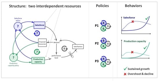
The generic policies discussed here refer to the simplest possible case of interdependent organizational resources, which comprises three internal and one external resource. The first internal resource is used to increase demand and represents the variety of marketing and advertising activities; it will be referred to as salesforce to avoid unnecessarily abstract language. The second internal resource—production capacity—summarizes all that is necessary to deliver according to the demand, so that customers will not be deceived and shift their demand to competitors. The third resource is external: demand is a sign of the customers’ satisfaction—the organization cannot directly control it, but it is necessary to keep the organization going [38]. Financial resources are the fourth resource (internal); they are a consequence of demand and necessary to fund the salesforce and production capacity.
The three generic policies are:
- Generic policy GP1: Drive growth through increases of the salesforce and adjust production capacity as needed.
- Generic policy GP2: Drive growth by investing in production capacity and adjust salesforce as needed.
- Generic policy GP3: Drive growth through simultaneous and harmonic increases of both salesforce and production capacity.
Generic policy GP1. If the salesforce can grow faster than the production capacity, it may be intuitive to use the salesforce as a driver for growth and adjust the production capacity as necessary. For many small and medium enterprises—especially in the developing world—the investments necessary to increase production capacity are huge and risky: one must mobilize financial resources incurring and long-term obligations without having the certainty of a sustained growth in demand. However, a policy that increases the salesforce and postpones increasing production capacity until the increased demand puts significant stress on the production capacity. It may not adjust the production capacity on time, deceiving customers and then facing a decreased demand when eventually the production capacity has grown [39,40].
Generic policy GP2. For growth-oriented companies that are not afraid of this risk, have huge fundraising possibilities, or important capital reserves, early and substantial investment incapacity has been recommended because of several reinforcing effects enabling sustained competitive advantage; there is a thin line between getting big fast and getting too big too fast [24,41,42,43]. The importance of developing sufficient capacity has been stressed [41], but “overshoot and collapse” as well as other cyclic instabilities continue to challenge managers. The delicate balance between the firm’s resources is still an important issue management education [40].
The perception and relative importance attributed of (1) the risk of long-term depth and financial hardship and (2) the risk of failing to increase the capacity on time will depend on the particular context of an organization’ founder or manager. Some may perceive the first risk more clearly than the second one, others may perceive both risks but value them differently. The studies concerned with the “misperception of feedback” suggest that individuals do not perceive the second risk because of the time delays.
Generic policy GP3. When prompted to choose one of these two policies, naïve individuals (without specialized knowledge) may also suggest that they would rather not use salesforce or production capacity as growth driver and adjust the respective other resource but drive the increase of both resources in the same way as maintaining the necessary synchronization.
Each of the generic policies GP1, GP2, and GP3 has been operationalized as specific policies P1, P2, and P3 (when the text mentions “policy,” it is shorthand for “specific policy”) and implemented as a simulation model inspired by a classic system dynamics model which is prominent in system dynamics and management education [39,40]. Comparison of the resource behaviors over time and the performance in terms of growth reveal that all three generic policies can generate an itinerary of sustained exponential growth, albeit policy GP2 allows to reach a stronger acceleration and much higher performance. This suggests that neither of these policies can avoid a “boom and bust” pattern if decision-makers can implement the chosen policy with carefully chosen parameter values.
The contribution of this article is therefore that all three generic policies can achieve sustained growth and do not necessarily lead to overshoot and decline or other undesired behaviors emphasized in the extant system dynamics literature. Despite the stronger performance of policy GP2, which implies the risks inherent of huge investments in the resource that grows only slowly, GP1 and GP2 are reasonable alternatives for decision-makers who prefer to avoid these risks. Due to the theoretical nature of this study, this contribution should be taken as conceptually valid but awaiting empirical data, and the system dynamics model used here is freely available for lab experiments.
The remainder of the article starts with a section which introduces a stylized decision situation involving three resources and the relationships between them, outlining the three generic policies. The ensuing section presents the specific features of the decision situation used in the simulation model and compares the results obtained by each of the policies. Based on these results, the fourth section proposes a revision of how the generic policies have been interpreted in previous studies, leading to a series of questions for theoretic and empirical research.
2. Theory: A Three-Loop System
2.1. The Structure and Dynamics of a Three-Resource System
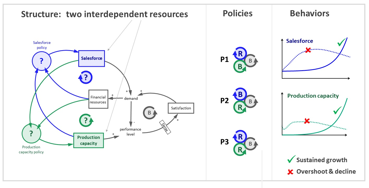
Consider a system comprising two agents: a company and customers. The company supplies a product that customers need or want, and the customers compensate the company with a payment, which is what the company needs or wants. Each of the two agents has something that the respective other agent wants and wants something that the other agent has. Both will interact as long as this relationship is reciprocal. If the company has been recently created, the relationship does not exist yet because the customers do not know that the company can supply something they want. Therefore, one of the challenges for the company is letting the customers know and desire the product. The necessary processes will only take place if the company has sufficient salesforce to fuel them. Assuming these processes are successful, the company will perceive an increasing demand for their products. Now, this growing demand must be satisfied. Again, the necessary processes will only take place if the company has sufficient production capacity. Failing to produce and deliver will lead to a decrease in demand.
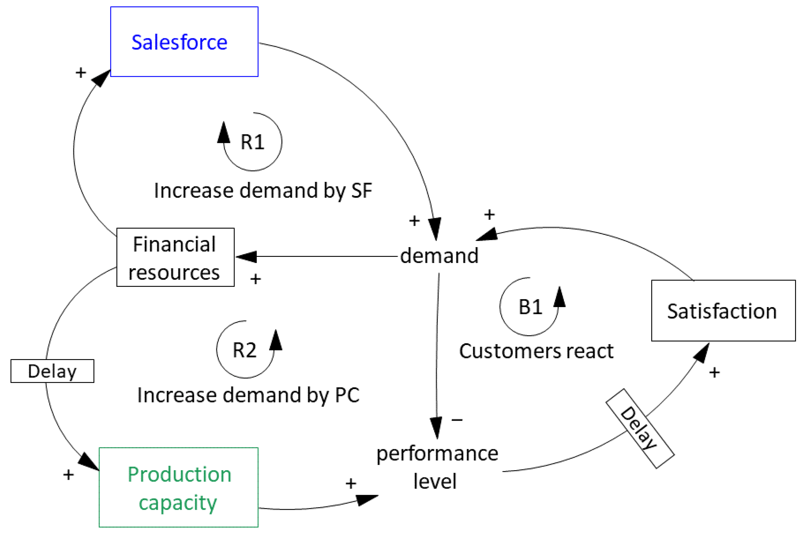
This fundamental structure can be conceptualized as a dynamic system as illustrated in Figure 1, where each of the agents is represented as a dotted rectangle: the company (left) and the customers (right). The figure contains a causal loop diagram [44,45] comprising feedback loops, variables, and causal links which are part of the decision situation regardless of decision-makers’ policies. Loops are marked by a circular symbol containing a letter “R” for reinforcing feedback and a “B” for balancing feedback. Two kinds of variables are visually distinguished: stocks appear in solid rectangles, and other variables simply appear with their name. The arrows between variables are causal links with a polarity sign and a delay mark where the relationship between two variables is delayed with respect to the other relationships. Positive polarity means that when the independent variable increases/decreases, the dependent variable’s behavior will change upwards/downwards. When an increase/decrease in the independent variable leads to a downward/upward change of the dependent variable’s behavior, polarity is negative.
In Figure 1, both agents interact through two variables: the customers signal their satisfaction through their demand and perceive the company’s performance level. Loop B1 represents the customers’ reaction to the performance level they perceive. The process of perceiving consists of gradually adjusting the perceived level to new signals over time. Changes in the performance level will take some time to trigger the corresponding changes in the level of satisfaction, which will slowly respond to an increasing or decreasing performance level by an increase or a decrease of satisfaction. Increasing satisfaction leads to increasing demand, just as a decrease in satisfaction triggers a decrease of demand. The relationship between demand and performance level is different: an increase in demand will lead to a decrease in the performance level, given the current production resources. This also means that a decrease in demand helps to increase the performance level. Therefore, when customers turn away from a company and the demand decreases, this is one way to correct problems at the performance level. However, from the standpoint of the company, this is an external correction—it cannot be directly controlled—a loss is the opposite of what a growth-oriented company aims for.
Inside the company, increasing demand leads to an increase in financial resources and decreasing the demand leaves the company with less financial resources than would have been the case otherwise. Other than this relationship and the causal influence of production capacity on the performance level and of the salesforce on demand, nothing is specified: the way how the company reacts to changes in its financial resources and how it will steer the two resources driving its relationship with its customers will be specified by the policies. The three distinct possibilities for steering each of the two resources are three different ways to connect salesforce and production capacity to demand, creating two feedback loops connected to the “customers react” loop. Growth drivers are self-reinforcing processes based on reinforcing feedback loops, whereas adjustments are control processes driven by balancing feedback loops [44]. Therefore, the generic policies are formulated as three different pairs of feedback loops, as shown in Table 1.
Regardless of which generic policy steers salesforce and production capacity, both resources are interdependent. An increase of the salesforce stronger than the increase of production capacity will put stress on production capacity, making it ever more urgent to increase production capacity because the additional demand decreases the performance level and risks to lead to decreasing satisfaction and demand soon. An increase of production capacity stronger than the increase of the salesforce will have two consequences: (1) It puts stress on the current salesforce to generate the additional demand which can now be attended to; and (2) it makes it easier to recruit additional salespeople because the increased capacity will cause satisfaction to increase, which increases demand and leads to increased sales revenues, also increasing financial resources and the budget for salesforce salaries.
2.2. Different Generic Policies to Develop Resources in This Context
2.2.1. Generic Policy GP1: Drive Demand Growth with the Salesforce and Adjust Production Capacity When Needed
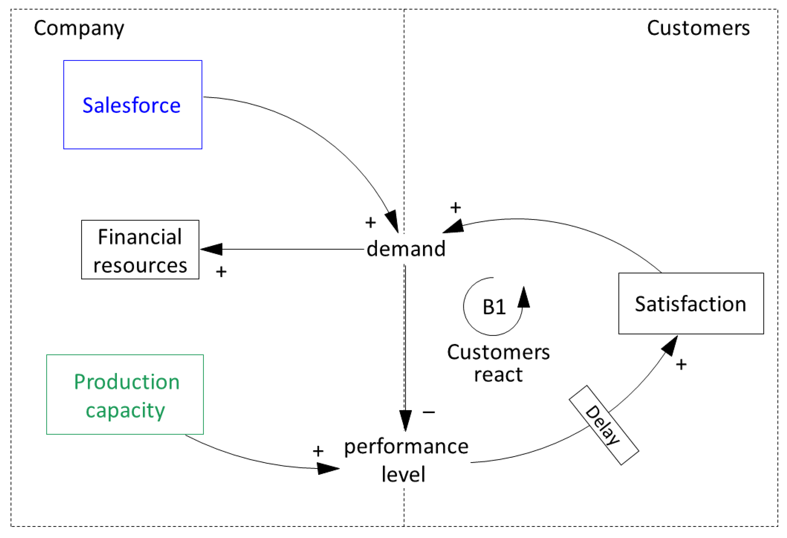
Policy GP1 consists of one set of rules for salesforce development which operate as a reinforcing feedback loop which we will refer to as R1, and another set of rules for developing production capacity which is a balancing loop with the identifier B2.
The reinforcing loop “increase demand” (R1) contains the positive link from demand to financial resources. Any increase or decrease in the stock of financial resources triggers a change with the same sign in the salesforce: more money automatically leads to more salespeople and decreasing financial resources entail decreasing salesforce. Changes in the salesforce cause changes of demand with the same sign: an increased or decreased number of salespeople always leads to an increase or decrease in demand. This loop is reinforcing and will always accelerate change in the direction of increase or decrease unless this behavior is limited by other factors. However, there are two more loops connected to it—directly or indirectly, as illustrated in Figure 2.
Figure 2 also shows the “sustain demand” loop (B2), which is internal to the company and sensitive to the performance level. The company compares the available observations of the performance level to a desired performance level. The delay between actual performance level and its perception by the company is because of the regular administrative processes. If the company perceives a gap between the desired and the observed performance level, it will adjust its production capacity. For instance, if the performance level has decreased, then the perceived gap increases, and therefore production capacity will be added to current stock. Increases in the observed performance level will reduce the gap, and it is even possible that a surplus of production capacity constitutes a negative gap, leading to a reduction or production capacity—a way to reduce costs that are apparently unnecessary. As argued earlier, the decision-maker can perceive this as less risky than making important investments in production capacity before demand actually increases. In such a case, it seems logical for the company to be cautious with the financial resources and therefore to only correct decreases in the performance level by increasing the production capacity.
Any additional production capacity must be ordered, constructed, mounted, and put into service before it can be used: there will be a sizable delay. As soon as the additional production capacity goes online, the company’s performance level will increase (momentarily assuming an unchanging demand). This is a balancing loop that will control the level of production capacity, such as to keep performance level close to the desired performance level.
The “sustain demand” loop (B2) is linked with the “customers react” loop (B1) by the performance level. Both loops use one variable to control the performance level. The company needs to correct performance level gaps before customers will adjust their satisfaction level: if the satisfaction level can decrease quicker than the production capacity can be increased, internal corrections to the production capacity will come too late. Moreover, note that there will be no increases of the production capacity unless a gap is perceived. This can only happen when demand grows faster than the production capacity—for a constant level of these resources, any increase of demand has this effect. It can even happen that a strong reaction of the customers, entailing a strong decrease of demand, increases the performance level so strongly that the company erroneously detects a need to decrease its production capacity. Since such a decrease of production capacity might also decrease the performance level, a reinforcing process might take over: in combination, loops B1 and B2 are a reinforcing feedback loop.
2.2.2. Generic Policy GP2: Enable Demand Growth through Production Capacity and Adjust the Salesforce When Possible
One way to avoid the vicious side of the first policy is to prioritize the increases of the production capacity and assure that the effect of an increasing salesforce will not unintentionally lead to a decrease in the performance level. This is a different approach to sustaining demand, and it is shown in the following Figure 3.
The causal loop diagram in Figure 3 contains the same basic structure (loop B1 and salesforce impacting the performance level through a positive causal link), but the logic of steering the internal resources is inverted. Changes to the financial resources drive the development of production capacity, whereas the salesforce reacts to perceived surplus performance—a gap between the observed and the desired performance level—such as to control the performance level. In this configuration, the “sustain demand” loop adjusts salesforce and the “increase demand” loop drives production capacity.
This configuration will increase the salesforce only when an increase of the production capacity has already increased the performance level, which means there is a surplus performance capacity which will remain unnecessary until additional salesforce can increase the demand such as to press performance level back to its usual value. Where policy P1 will be late to adjust the production capacity, policy P2 accepts the effect of spending “too much” money for production capacity—as compared to the level of demand—a sacrifice for being able to produce sufficiently once the increased salesforce has led to a demand which with fully require the increased production capacity. The fact that the “customers react” loop is quicker to impact performance level than the “sustain demand” loop is not a danger here because changes to satisfaction will only be triggered when the change of production capacity has already happened. For decision-makers who do not mind the perceived risk of being unable to increase demand sufficiently, being able to avoid a loss of satisfaction caused by insufficient production capacity will make policy P2 attractive.
So, even though P2 can generate sustained and accelerating increases of demand, it also contains the possibility of an accelerating decrease.
2.2.3. Generic Policy GP3: Drive and Enable Growth Simultaneously
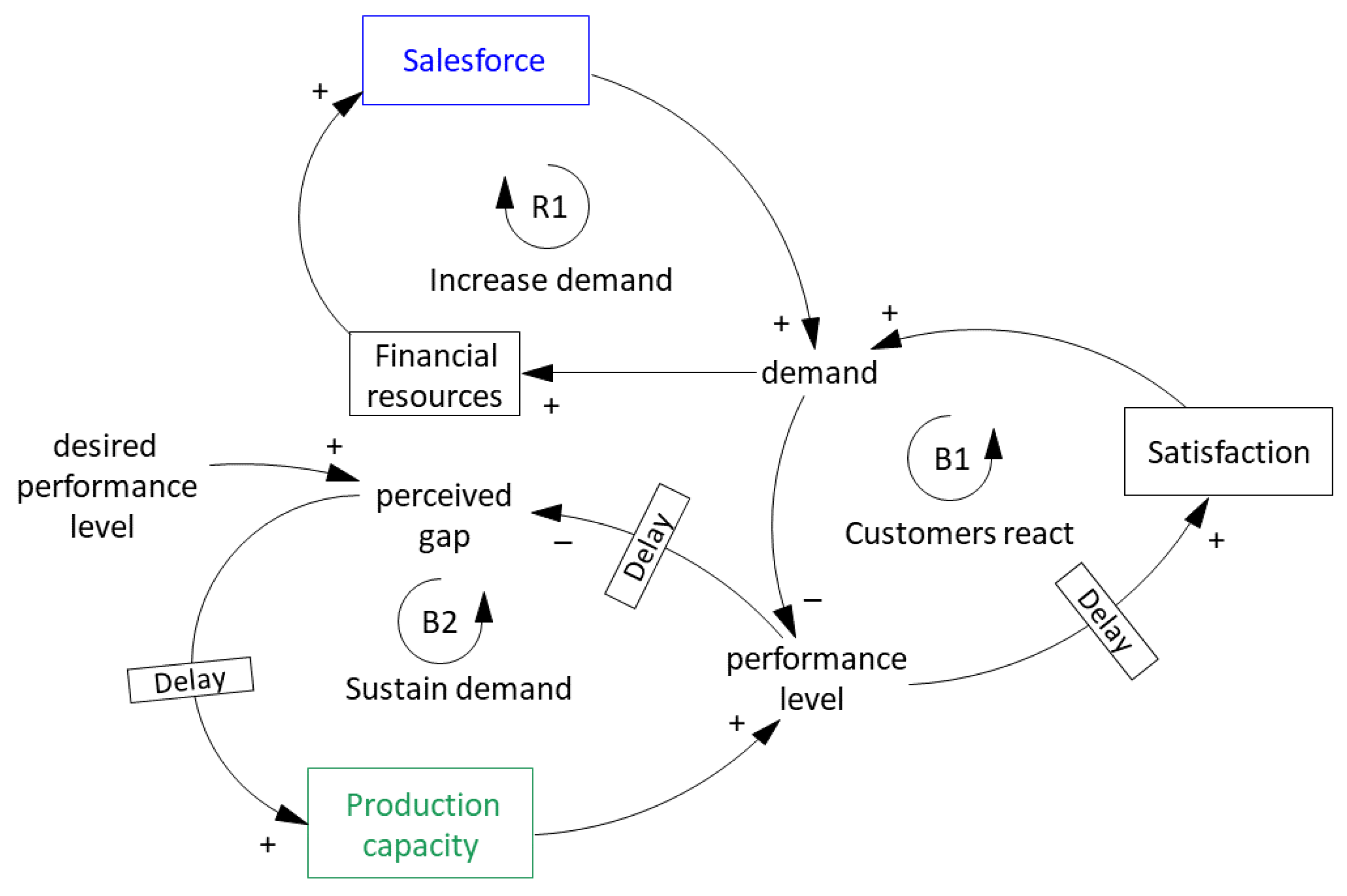
Decision-makers who are aware of the risk inherent in policy P1 and find themselves unable or unwilling to make important investments ahead of possible increases of demand (P2) may consider a third possibility: use increases in financial resources to increase the salesforce and production capacity simultaneously. This logic is shown by the causal loop diagram in the following Figure 4.
The structure shown in Figure 4 conserves the “customers react loop.” The causal link from demand to performance level belongs to two different loops, and so does the link from demand to financial resources. Now, both loops internal to the company are reinforcing in nature. The company’s logic of steering the salesforce is the same as in policy P1, and its way to steer production capacity is the same as in policy P2. Since “increase demand by SF” (R1) as well “increase demand by PC” (R2) are reinforcing, it can indeed happen that the potential decrease of performance level in response to an increased demand is exactly compensated for by the effect of additional production capacity on the performance level. Therefore, demand could indeed grow quickly—accelerating—and be sustainable. Achieving such steady and accelerating growth requires that the company be able to determine which fraction of additional financial resources is used for salesforce and which fraction is to be used for production capacity. Of course, such a growth would still be limited by overall size of the market and the market share captured by the company. However, this limitation is the same for all three policies, and unless the limit is reached, its theoretical existence does not make a difference through the choice among these three policies.
3. Method
3.1. Description of the Specific Decision Situation Used in the Simulation
Section 2 has discussed the generic policies GP1, GP2, and GP3. In the current section, specific policies P1, P2, and P3 will be introduced as an operational instance for each generic policy. Each policy will be simulated, and its behavior and performance analyzed and later used to compare the generic policies. This subsection introduces the necessary details of each policy; aspects beyond the scope of this discussion of the policies discussed here can be interactively examined using the freely available on-line simulator described in Appendix A, and the exact formulation of the simulation model is reported in Appendix C.
The following description of the decision task contains the aspects needed for the theoretic inquiry discussed here; a more detailed description for hypothetical participants in an experiment is provided in the Supplementary Materials. Decision-makers take the role of a manager who has been recruited by a young company which produces and distributes customized watches. The manager will be responsible for a new division which has been launched recently with a planning horizon of around 10 years. The short-term goal is to achieve a strong and sustained growth in terms of sales over a period of 50 weeks. When taking office, there are 40 salespeople and up to 1512 weekly watches can be produced.
For the sake of simplification, customers are assumed to care only for the delivery delay—the number of weeks between placing an order and the delivery of the watch—with a delivery delay of two weeks. This delay assures that salespeople can sell at 90% of their maximum productivity: 9 new orders per week. The company might increase customers’ willingness to buy to 100% by becoming quicker to deliver, but the loss of demand caused by becoming slower to deliver is more drastic. It follows that the price of €431 does not bother customers, and therefore the price stays constant during the entire game. The initial weekly production capacity of 1512 watches (with 21 shifts) assures that the open orders—720 at the beginning—can be delivered in this delay, and the salesforce of 40 individuals will be able to produce 360 new orders per week.
Each week, several decisions must be taken. The first is the recruitment or layoff of salespeople. Recruiting salespeople takes somewhere between one and four weeks depending on the number of salespeople to be recruited. To simplify, €3000 is the fixed salary for all salespeople (no incentives), and they all have the same productivity, being able to bring in a maximum of 10 new orders per week. The salesforce is limited by a budget rule: not over 25% of expected sales revenue can be used for salesforce salary. If there has been an increased number of deliveries, 25% of the additional revenue will be available for recruitment, and the manager decides which percentage of this to use.
For production (including delivery), the weekly number of producible watches depends on the production capacity and on the capacity utilization fraction (CUF), which is the actual weekly number of shifts divided by the maximum weekly number of 21 shifts (3 shifts for 7 days): the number of daily shifts times the number of labor days per week. Late or night shifts and work on weekends cause increased salary costs. But modulating the CUF allows to increase effective production without investing in additional production capacity up to a certain point. There is a capacity construction delay of eight weeks: capacity orders in week w will only come online in week w + 8.
There’s also a budget limit for spending money on capacity increases: participants are informed of a maximum weekly amount and can decide which percentage of this to use. This additional capacity spending is determined by the difference between the production capacity needed to produce and deliver 50% of the open orders (such as to assure delivery in two weeks) and the current production capacity, multiplied by the unit cost of production capacity. Note that this allows the manager to order all additional production capacity needed to maintain the delivery delay—or less. Additional production capacity for 1 weekly watch costs €20,000 and works for 8 years, which is equivalent to 416 watches. This makes roughly €48 per watch. The total costs for producing and selling one watch range from €283.33 to €333.33, depending on the capacity utilization fraction.
At the sales price of €431, there remains a difference of between €147.67 and €97.67 per watch, so over the lifespan of the production equipment, profits are assured. However, it is impossible to fully compensate the initial investment costs by sales revenues in as little as one year.
3.2. Benchmarks for Comparing Possible Policies
3.2.1. The Classical Example of Market Growth and Underinvestment in Capacity
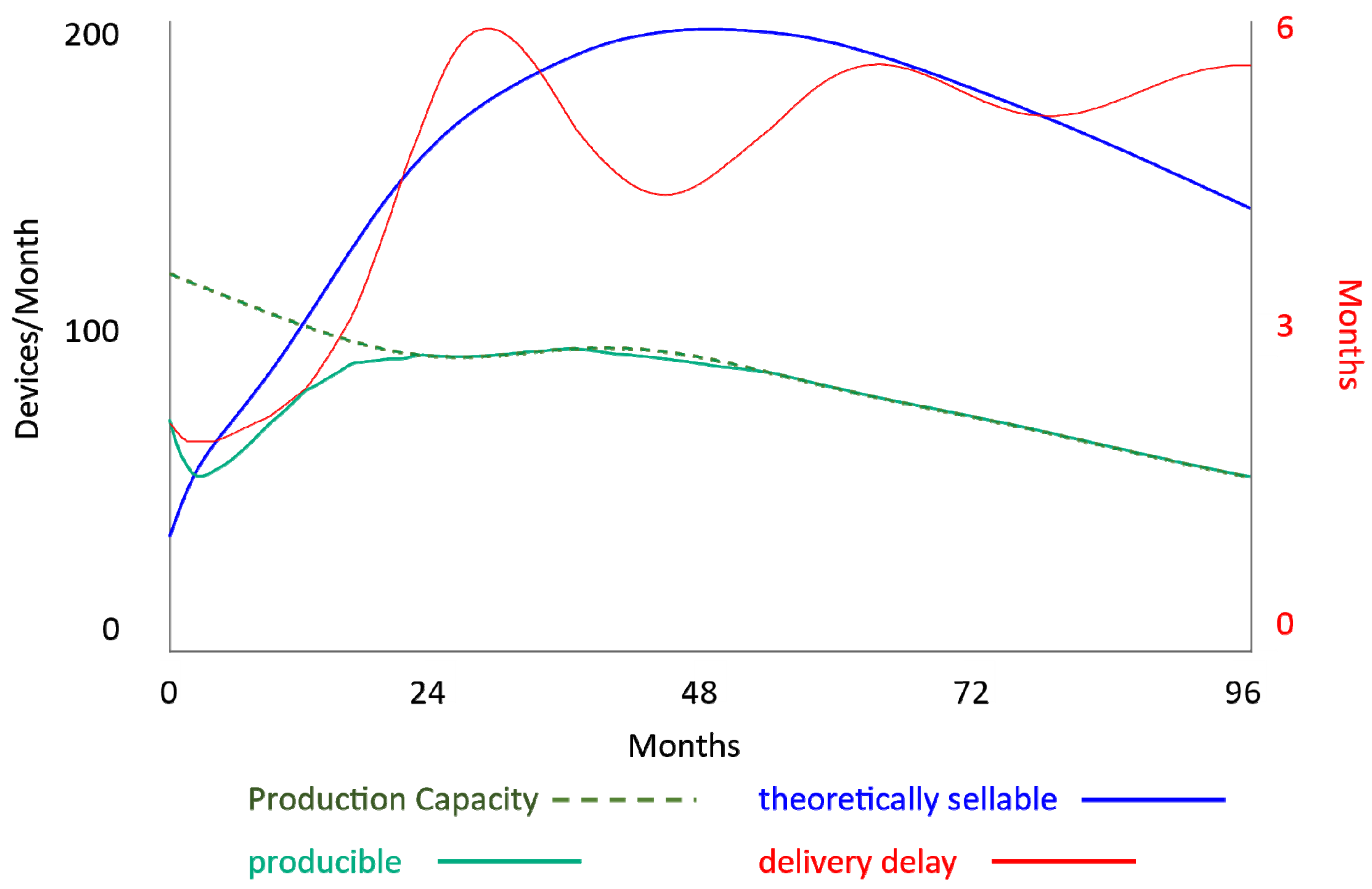
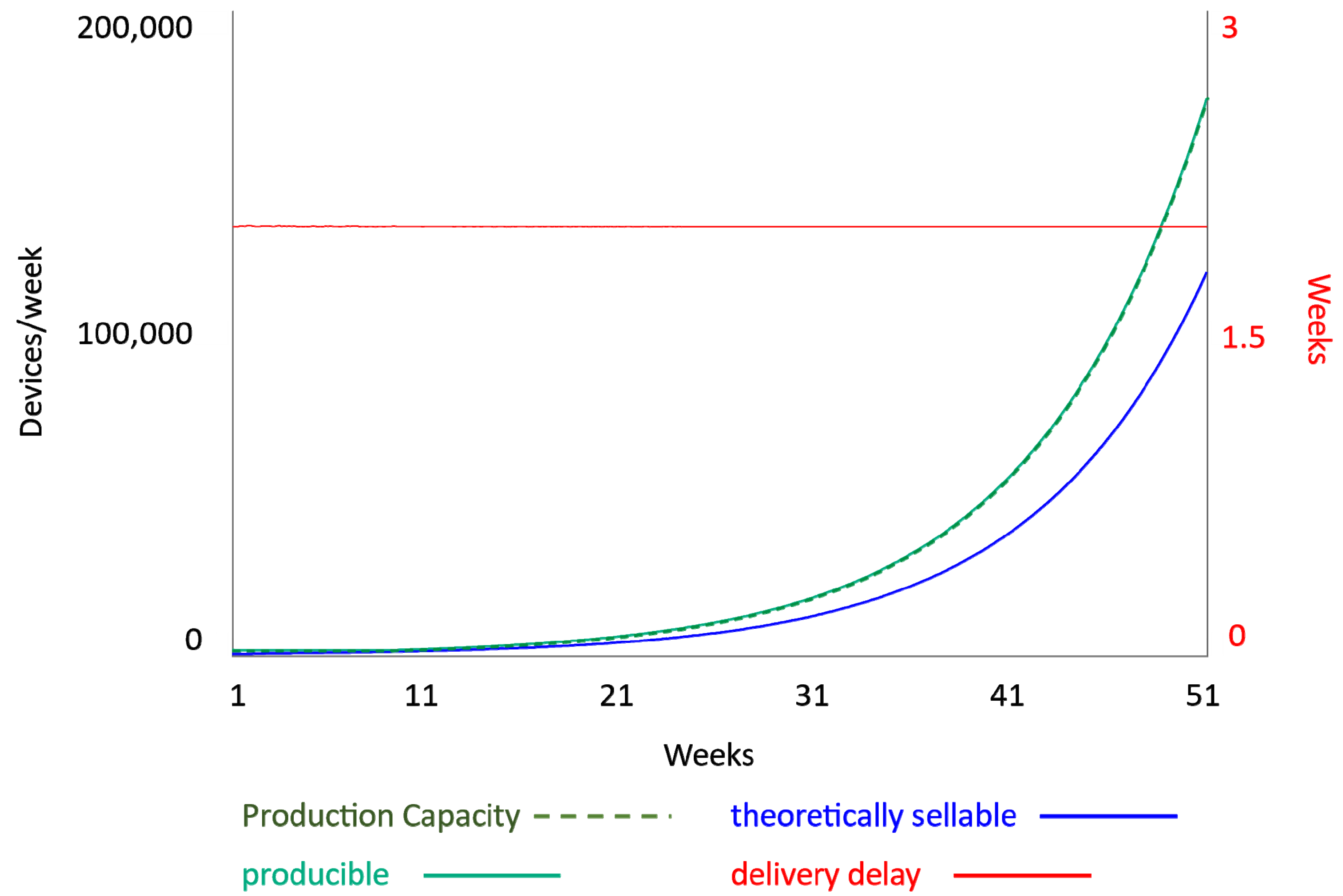
The case used here is a simplified version of the “market growth and underinvestment” case [39,40], which dealt with a company producing navigation devices for boats and had a time horizon of 96 months (8 years). This company followed policy GP1. Compared to our case, it included a fourth feedback loop representing eroding goals because the workers in the production facility get used to longer delivery delays and do not feel the urgency to produce in less time. When management demands funds for additional production capacity, headquarters discounts a certain fraction. The underlying simulation model generates an initial episode of growth which quickly turns into a steady decline, as shown in Figure 5 (graphic elaborated by the authors based on the model published in [40]):
Figure 5 shows the monthly number of devices the salespeople can sell, assuming their regular productivity and the monthly number of devices the company can produce. The production capacity is a dotted line, and together with the capacity utilization fraction (CUF), it determines what is actually producible. In the “market growth model,” the CUF is also a multiplier which is adjusted between 0 and 1, and it modulates which fraction of the production capacity is used—adjusting such as to avoid using more capacity than needed to fulfill orders in the delivery delay. Since the effect of the CUF is immediately visible in the difference between production capacity and producible, the CUF is not included in the diagram to avoid cluttering. The key features of this behavior are the rise of the delivery delay and its oscillations, the decrease of the producible quantity of devices, and the boom and bust of the sellable quantity of devices.
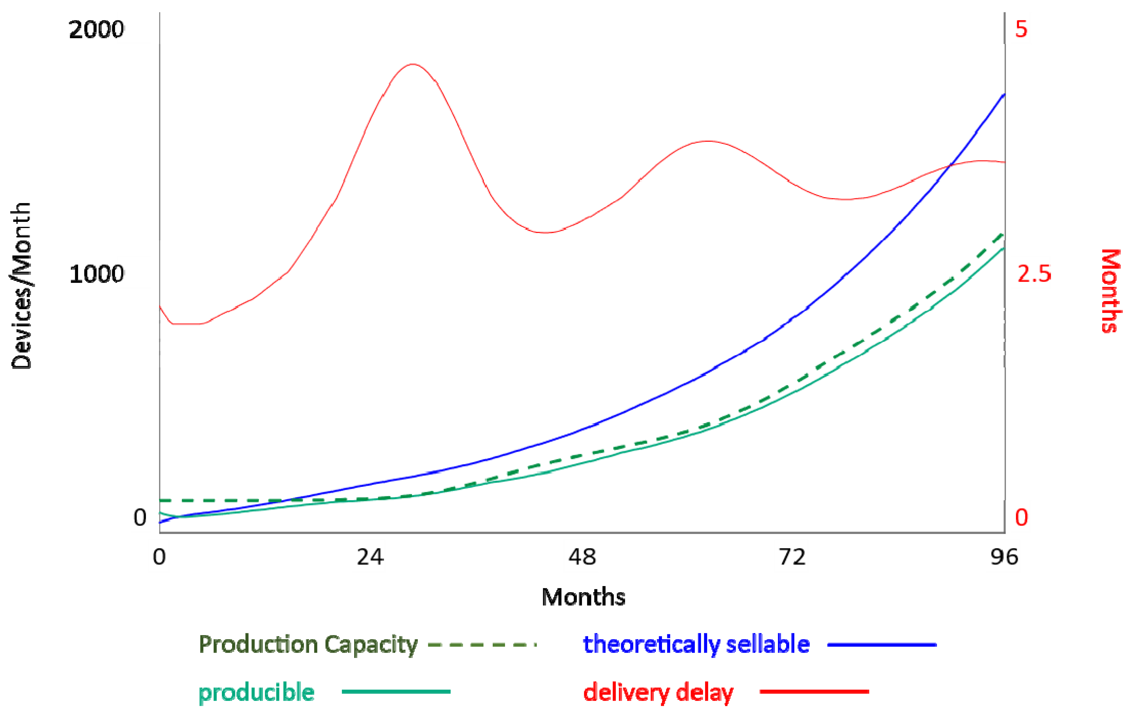
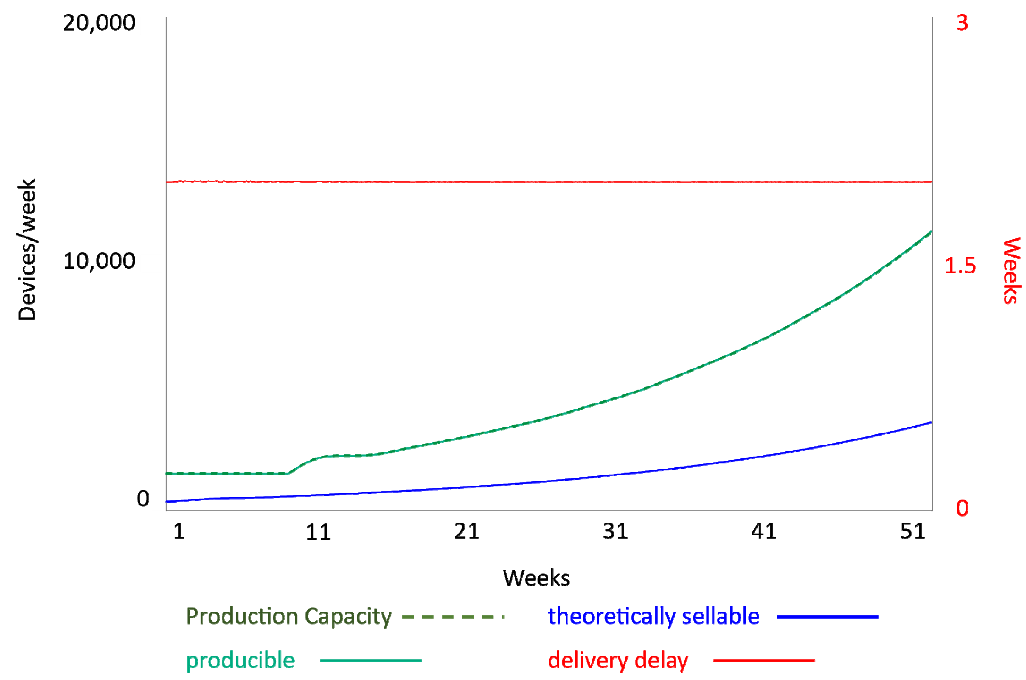
When the fourth loop (eroding goals) and the discount of funds for additional production capacity are taken away, the behavior changes as displayed in Figure 6.
As shown in Figure 6, the delivery delay still oscillates and it still increases to somewhere near 3.5 months, which is better than the initial 6 months but still is not what the company wishes to achieve. The decrease of the producible quantity has not turned into a moderate exponential growth. The sellable quantity also grows exponentially—with minor oscillations along its path—and at the end of the 96 months, the salesforce could reach up to 1700 monthly new orders, while around 1000 monthly watches are producible. Even in these conditions, the policy fails to steer the company on an itinerary where delivery delay = desired delivery delay. The increased delivery delay turns customers off and a constant number of salespeople will generate less new orders, implying increased salary costs per unit sold.
3.2.2. How to Include the Interdependency between Salesforce and Production Capacity in Specific Policies
The policy embedded in the “market growth” model is the substrate of observations made by Forrester [39] in actual companies. Even if one can assume the decision-makers in these companies were aware of the fact that it takes more time to adjust the production capacity than the salesforce, it is unknown how exactly they took this into account their decisions. In contrast, the three policies discussed here exploit facts known from the case description transparently.
The stress put on the production capacity due to an increasing salesforce can be used to determine the recommendable quantity of additional production capacity, because production capacity should be sufficient to produce 50% of the open orders per week to assure that the desired delivery delay will not be over 2 weeks. For this, assume that total production capacity = production capacity + capacity under construction: taking additional capacity that has been ordered but is not yet online is necessary to avoid oscillations [14].
The reasoning is represented by the five following simple equations:
Desirable deliveries = open orders/desired delivery delay
Theoretically producible = total production capacity * capacity utilization fraction
Capacity fractional effort = (desirable deliveries/theoretically producible)/2
Capacity indicated by effort = total production capacity * (1 + capacity fractional effort)
Capacity adjustment indicated by effort = capacity indicated by effort − total production capacity
A stress level of, for instance, 5% would suggest that 5% additional production capacity needs to be ordered. Decision-makers can take such a recommendation into account, but they are not forced to fully do so: it can be applied partially as well as fully. There are different ways to use this reasoning, as discussed in the following subsections.
3.2.3. Specific Policy P1
A player who follows policy GP1 would want to use 100% of the available budget for reinforcing the salesforce and order additional production capacity as needed. “As needed” needs to be specified in detail. One intuitive possibility is to react to resulting increases in the delivery delay, but this is a reactive tactic which requires the decision-maker to wait until the delivery delay increases before it can be corrected. The abovementioned possibility calculates the additional production capacity required to produce the additional new orders to be expected due to the new salespeople.
Note that both alternatives make no mention of the different delays for actually becoming able to use the additional salesforce and the additional production capacity. The question arises if even the second possibility—presumably less reactive—implies the risk of overselling and under-producing. For instance, if the company looks for an additional 20% salespeople—an increase from 40 to 50 individuals—this will only take one week. As soon as these new salespeople place their 90 weekly new orders, 45 additional units of production capacity are needed. But if they have been ordered together with the additional salesforce, seven more weeks will pass before these capacity units come online. In the meantime, 630 additional new orders would have been added to the open orders, progressively increasing the delivery delay. Since the perception process of customers takes less time than building the new production capacity, demand would already have diminished, so that there would be less than 630 additional new orders: the “customers react” loop would correct the problem of insufficient production capacity before the company can do so.
Additional complexity comes from the fact that increases of the capacity utilization fraction also can absorb a certain amount of additional new orders. But as the weekly number of shifts approaches 21, this possibility melts away. Still, it is useful as a short-term absorber of the relatively sluggish growth speed of production capacity, but not as a replacement for investments in additional capacity.
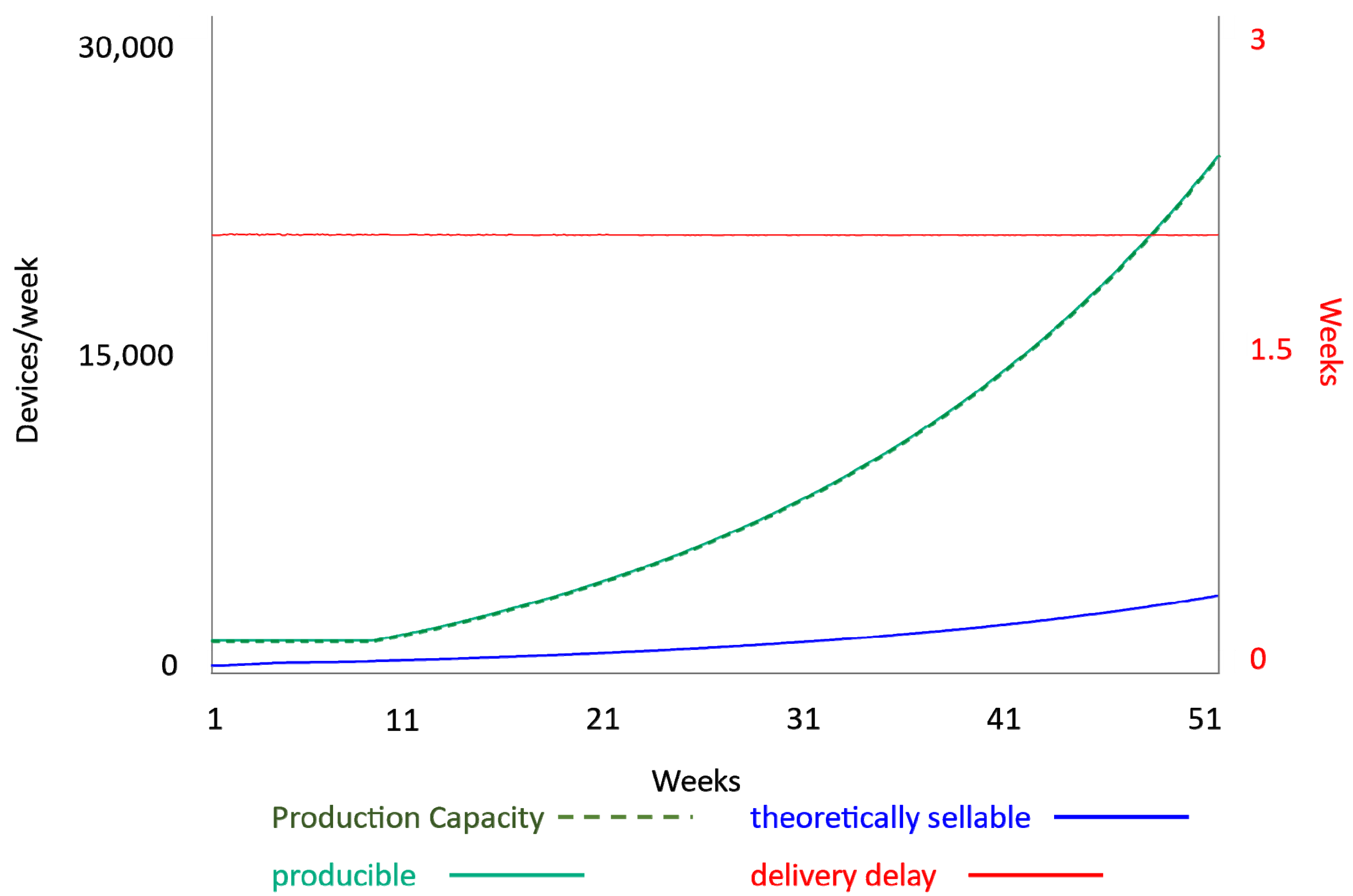
However, simulation reveals that policy P1 avoids this risk. If the decision-maker (1) always uses the full salesforce recruitment budget and (2) always orders additional production capacity such that the resulting total production capacity would be sufficient to produce and deliver all open orders within the regular delivery delay (assuming 100% capacity utilization fraction), then sales, salesforce and production capacity would display a slightly accelerating (exponential) growth at a constant delivery delay of two weeks, as shown in Figure 7.
Figure 7 also shows that the production capacity exceeds the quantity of theoretically sellable watches, and increasingly so. The specific behavior and numeric values displayed depend on a policy implementation fraction: how strongly the decision-maker converts the recommended change of production capacity in actual orders of additional capacity. On a scale from 0 to 1, a value of 0.2 leads to the lowest amount of overcapacity without diminishing the total number of watches sold (0.1 leads to under-investing in production capacity and would not be sustainable after the end of the year; the simulator described in Appendix A allows to explore the behavior and performance according to varying values of the policy implementation fraction). The company would therefore not need to run all 21 weekly shifts (CUF = 100%) to produce sufficiently.
At the end of the year, 398 individuals would be in the salesforce, being able to sell 3585 watches, and the production capacity of 5930 would be 2344 watches or 65% higher than necessary (assuming CUF = 100%). The company would have delivered 66,283 watches; as compared to the 17,280 watches sold without sales growth, this is over 1.8 times more and corresponds to a monthly growth rate of 9%. The accumulated overcapacity represents all capacity units that exceed what the salesforce can sell over the 50 weeks, and it amounts to 68,859 watches. Overcapacity implies that the company has invested more financial resources in production capacity than what would have been necessary to fulfill the open orders in the desired delivery delay. Together with the accumulated deliveries, it allows to judge the policy’s performance compared to alternative policies.
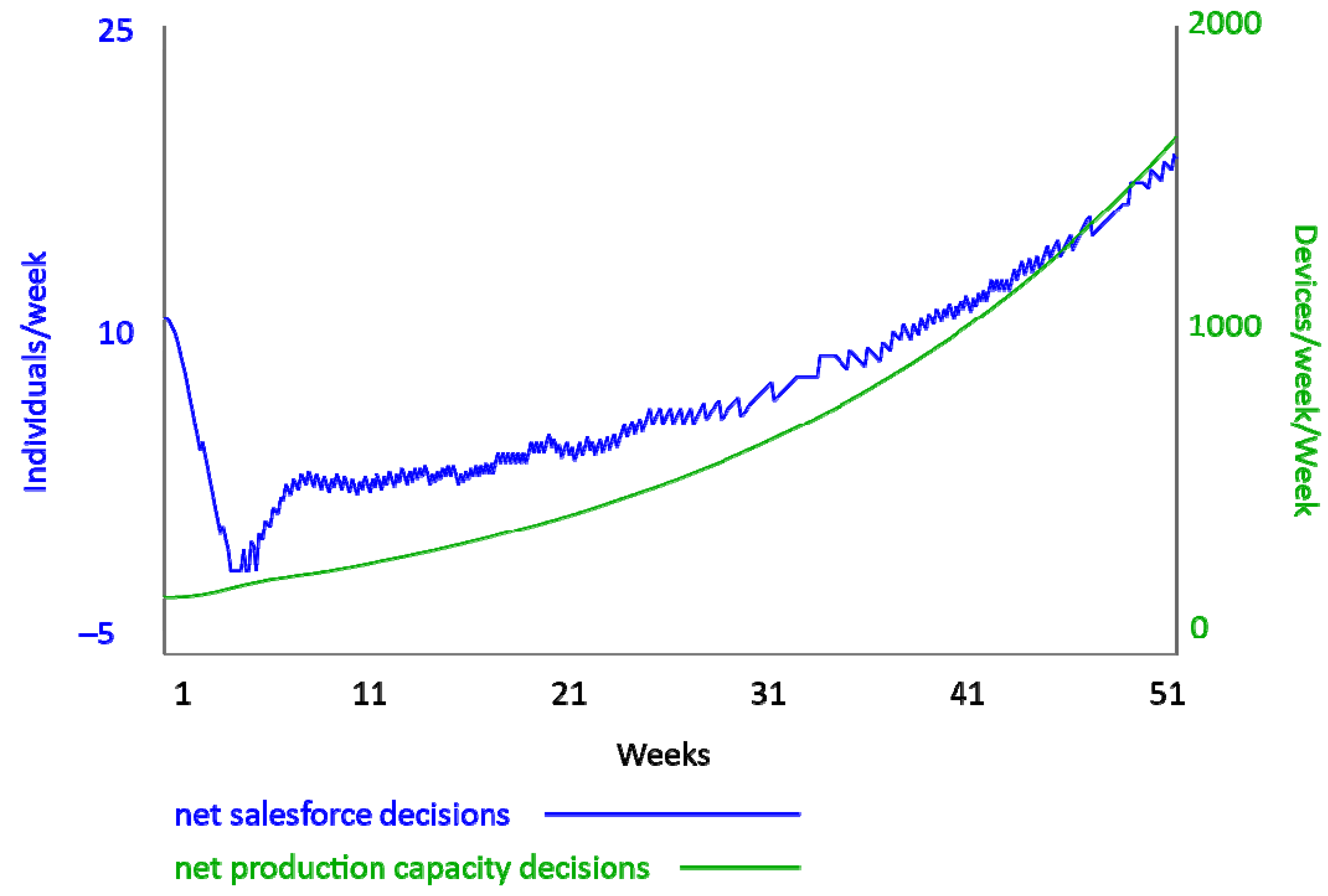
The stream of recruitment decisions driving this development is a continuous curve for production capacity and zigzagging for salesforce; this is a consequence of binding salesforce recruitment to a constant fraction of the expected sales revenues which can rise one week and then fail to keep rising the following week because production capacity could not be increased immediately. This is displayed in Figure 8.
A higher revenue fraction for salesforce salaries would allow to achieve more growth in both resources and to increase the accumulated deliveries: a quicker increase of the salesforce would also increase the stress on production capacity, leading to larger adjustments to production capacity. The revenue fraction for salesforce salaries is like a gain factor for the “increase demand” loop (R1) around the salesforce: the higher the gain, the stronger the growth of the salesforce and production capacity is adjusted by the “sustain demand” loop (B2).
For 50% and 75% respectively (instead of 25%), the salesforce at the end of the year would be 11,402 or even 29,698 individuals, and production capacity would amount to 56,539 watches per week. Accumulated deliveries would increase to 585,194 and 921,889 respectively. However, the delivery delay would increase to 3.5 and 5.3 weeks instead of 2 weeks, indicating that there is overcapacity and too much money has been invested in production capacity; additionally, the productivity of salespeople would sink from the usual 90% to 60% and 30%, implying an increase in the sales force salary costs for selling one watch. Decision-makers who follow general policy GP1 are likely to avoid increased costs, and especially so if a fraction of such additional costs would be unnecessary. Therefore, the default revenue fraction for salesforce salaries of 25% is retained as the P1 scenario for comparison with the other policies. Interested readers can explore these and other parameter values in the interactive simulator described in Appendix A.
3.2.4. Specific Policy P2
Players who reason according to generic policy GP2 will want to apply 100% of the feasible increase of production capacity and recruit additional salespeople as needed to avoid that the additional capacity remains idle. Overcapacity would mean that the company can produce more than it can sell, and that the delivery delay sinks below one week. This can be avoided by driving recruitment according to how much bigger the salesforce could be without becoming unable to fulfill the open orders in the delivery delay of 2 weeks. The idea of putting stress on production capacity discussed above is now applied to the salesforce adjustments:
Theoretically producible = total production capacity * capacity utilization fraction
Theoretic excess production capacity = theoretically producible − theoretically sellable
Additional salesforce for excess productibility = theoretic excess production capacity/sales productivity
This will avoid over-recruiting like in policy P1. However, the upper limit for additional production capacity depends on the relationship between the current total production capacity and the one needed according to the number of open orders. So, if there is no or only little growth in new orders, only little additional production capacity can be ordered. Therefore, it will be necessary to use a certain percentage of the allowed additional recruitments to assure just enough growth of new orders to obtain the possibility to make more investments in the growth of production capacity. Mentally computing a convenient percentage may be easier when one assumes 21 weekly shifts (CUF = 100%), but even so this task is cognitively taxing.
As with policy P1, there is a policy implementation fraction: if set = 0.7, the development of overcapacity is minimized, and the results are similarly shaped than the ones of policy P1, but at a much higher absolute level. In Figure 9, the strong growth requires adjusting scale of the vertical axis from 30,000 to 200,000:
Figure 9 shows that the delivery delay is 2 weeks during the entire year. The salesforce reaches 12,656 individuals, being able to sell 113,907 watches for a production capacity of 118,860 watches per week. This means only 4% overcapacity at the end of the year (implying the company must stick to 21 weekly shifts), and the accumulated overcapacity is 65,959. The accumulated deliveries amount to 823,596 watches, which is almost 50 times the baseline sales and implies a monthly growth rate of 38%. The stream of decisions concerning production capacity is as smooth as for policy GP1, but policy GP2 also generates a smooth stream of salesforce recruitment decisions.
This strong acceleration is enabled by the way how salesforce recruitment happens under P2. Whereas P1 steers this recruitment using the allocated budget, P2 depends on the theoretic excess production capacity (Equation (7) above). If the additional salesforce for excess productibility (Equation (8)) is greater than the payable additional salesforce, then P2 will generate a higher number of salespeople than P1. Indeed, comparison of the salesforce costs for P1 and P2, respectively, reveals a difference right from the first week on, as shown in the following Table 2. The table displays time in rows and contains the salesforce salary costs of the initial four weeks under policies P1 and P2 as columns. Some additional values of the revenue fraction for salesforce salaries (which by default is equal to 25%) for P1 lead to different behaviors: columns P1 50% and P1 75% show the costs when policy P1 is followed assuming that the revenue fraction for salesforce salaries be 50% and 75%, respectively. Column P2 limited refers to using policy P2 but limiting the recruitment by the payable additional salesforce under the regular revenue fraction for salesforce salaries of 25% (that is, like in policy P1).
All policies start under the same initial conditions in week 1, where the salary costs are EUR 30,000. Starting in week 2, P2 recruits more new salespeople than P1, and after four weeks, this difference is approximately 25%. Therefore, more salespeople are selling and make orders grow, which then enables to further increase the production capacity. This means that the reinforcing “increase demand” loop (R2) around production capacity drives the balancing “sustain demand” loop (B2) around the salesforce along its accelerating growth itinerary.
The previous section on P1 has discussed that the revenue fraction for salesforce salaries could in principle be increased by 50% or even 75%. Table 2 shows that this would generate a similar increase of the salesforce, as becomes visible from the salesforce salary costs in the third and fourth column of Table 2. However, the increase in costs—containing the costs of overcapacity and decreased salesforce productivity—make it unlikely that such an increase of the revenue fraction for salesforce salaries would be made by decision-makers who prefer GP1.
The last column of Table 2 shows what would happen if salesforce recruitment was limited to the revenue fraction for salesforce salaries of 25% which is used in P1 and P3. The salesforce would behave exactly like under policy P1; at the end of the year, 398 salespeople could theoretically sell 3585 watches per week (at a delivery delay of 2 weeks) but production capacity would be 16,974 watches per week, and accumulated deliveries amount to 66,284 watches. There would be a huge overcapacity, implying that huge financial resources have been invested in production capacity without generating sales revenue. This shows that the quick growth under P2 can be held up and become like what happens under policies P1 and P3, but it would be inefficient and decision-makers willing (and able) to make big investments in production capacity would be unlikely to implement this variant of P2.
3.2.5. Specific Policy P3
Decision-makers may use generic policy GP3 to grow the business with a convenient pair of percentages: use r% of the maximum allowed recruitment and a% of the maximum allowed additional production capacity. There are many such combinations, but only one will achieve the highest accumulated number of delivered watches—which is what the decision-maker is responsible for. One intuitive way to decide the proportion of allocated money is to reason with the unit productivity of both resources: if ΔSF additional salespeople can be recruited for a salesforce of SF individuals, the percentage of salesforce increase ΔSF/SF should be the same for additional production capacity ΔPC as percentage of total (current) production capacity PC:
ΔPC/PC = ΔSF/SF.
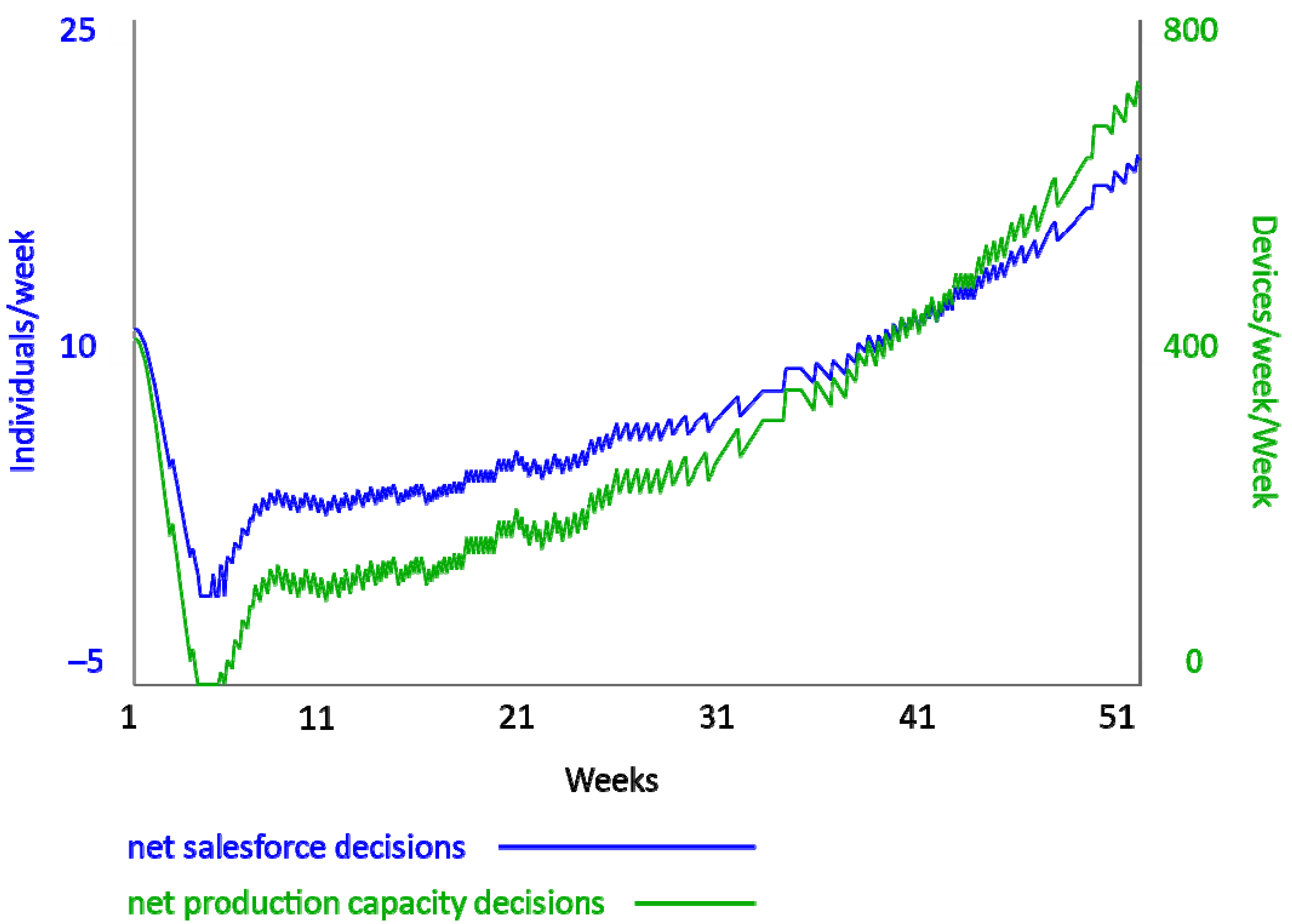
The result can then be transformed in the amount of money needed to order ΔSF and the amount needed for ΔPC. Following this idea with a policy implementation fraction of 0.7 (which minimizes overcapacity without reducing deliveries) in the simulation yields similar outcomes as policy GP1, as displayed in Figure 10.
Figure 10 illustrates how resources grow exponentially with a moderate curvature or acceleration, reaching a final score of 398 salespeople selling up to 3585 watches at a production capacity of 6200. At the end of the year, there is an overcapacity of 71%, meaning that for the same total quantity of deliveries—66,284—and the same monthly growth rate of 9%, the company has spent more financial resources than policy GP1 without need. This large overcapacity in the last week is a warning: even though over the year, the accumulated overcapacity is identical to the one observed in policy GP1 (68,723), the tendency is clearly “increasing,” and the following year ought to be viewed with worry. Therefore, while policy GP3 is sustainable, the unnecessary spending goes against the company’s goals and the decision-maker’s mission.
Regarding the decision streams of policy GP3, Figure 11 shows that there is an initial dip followed by a trend of moderate exponential growth with permanent week-to-week. This happens since production capacity needs six to seven more weeks than salesforce to react to the decisions made each week. After the initial weeks, this difference of time delays is no longer visible in the curve, even though each increase of production capacity in the upper graph is the consequence of a decision taken six to seven weeks earlier.
If P3 operates with alternative values for the revenue fraction for salesforce salaries, (50% and 75% of the expected sales revenues) similar changes like with P1 can be observed. The salesforce grows up to 9435 and 28,200 individuals, being theoretically able to sell up to 84,914 and 253,801 watches per week (summing up to 724,657 and 1,435,274 accumulated deliveries) for a production capacity of 35,744 and 70,105 watches per week. However, the delivery delay increases to 5.2 and 6.7 weeks—which can already be expected from comparing the number of theoretically sellable watches to production capacity. There is too little production capacity, which implies that salespeople can only sell 35% and 20% of what they would ideally sell (when the delivery delay is two weeks): this increases the salesforce salary costs per sold unit, and therefore, decision-makers following GP3 would be unlikely to adopt such high values of the revenue fraction for salesforce salaries.
4. Discussion
The following Table 3 summarizes key features of these three policies with their default values for the revenue fraction for salesforce salaries. The alternative values of the revenue fraction for salesforce salaries for P1 and P3, as well as the alternative formulation of P2 are not discussed here because they are unlikely to be applied by decision-makers (readers interested in these alternatives find the indicators and a discussion in Appendix B). These indicators are meant as benchmark for the behaviors and results of the participants in the experiment. The discussion takes specific policies P1, P2, and P3 as representing the generic policies GP1, GP2, and GP3.
The respective policy implementation fractions have been chosen such as to minimize the overcapacity that accumulates over the year: any other value leads to higher production capacity without increasing the total quantity of watches delivered. Generic policies GP1 and GP3 drive the salesforce identically and yield the same result for accumulated deliveries; however, GP3 performs slightly worse in terms of overcapacity: the theoretically sellable number of watches falls short of production capacity, which is equivalent to a production capacity surplus of 65% for GP1 and 73% for GP3. This implies that too many financial resources have been put into production capacity, which is equivalent to reduced profits. However, our primary criterion for assessing the qualities of these policies is the ability to generate sustained (exponential) sales growth, and profits would only make a difference if two policies perform equally well in sales growth.
The results achieved by policy GP2 are huge compared to the other policies, with a monthly growth rate four times as high. As discussed in Section 3, GP1 and GP3 could use an increased value for the revenue fraction for salesforce salaries to yield a higher sales growth, but this would also mean increased dis-balances between the selling capacity and production capacity, implying inefficient allocation of (scarce) financial resources. Moreover, increasing the revenue fraction for salesforce salaries over 30% leads to oscillating behavior of the delivery delay, revealing that the resource-increasing decisions generate imbalances which are compensated for, provoking new imbalances with the opposite sign. However, an analysis of these oscillations would be beyond the scope of the present article, and readers are invited to explore the effects of higher values of the revenue fraction for salesforce salaries using the on-line simulator described in Appendix A. One can also doubt whether a monthly growth rate of 38% can ever be reached or even sustained in real life: even if it was possible in the very short term, it would quickly attract competitors. However, competition is, as per assumption, left out of the theoretic and stylized decision situation studied here. However, even if the monthly growth rate was less than 38%, it would still be higher than the growth rates reached by GP1 and GP3. It is important to note that the logic behind policy GP2 leads to much higher growth rates, at least until the entry of competitors changes the entire decision situation.
All three policies allow for smooth and exponential growth, even though GP2 is much stronger, and the behavior pattern of both resources could be sustained beyond the end of the year: even GP1 and GP2, which maintain an overcapacity, can be defended arguing that the relative weight of the overcapacity decreases over time.
Whereas the behavior seen in the “market growth” case showed an increase of the delivery delay to almost twice the value of the desired delivery delay—even without the “eroding goals” feedback loop and without a diminished investment in production capacity (see Figure 6 above)—all three policies maintain the delivery delay equal to the desired delivery delay. This implies that even policy GP1, which follows the same line of reasoning as the “market growth” case, can be operationally specified such that production capacity is adjusted quickly enough to avoid overselling—which would drive the delivery delay up. By consequence, policy GP1 is not necessarily an idea leading to unsustainable growth followed by a decline.
A second difference in terms of delivery delay is that the three policies avoid the oscillations observed in the “market growth” case (at least for the default value of the revenue fraction for salesforce salaries). The fact that production capacity develops through two stages, modeled as two sequential stocks (refer to Appendix C for the equations), means that policy GP1 contains a second-order balancing feedback loop. When decision-makers overlook the delay implied by one of these stocks—in this case capacity under construction—they are led to take exaggerated decisions which later have to be compensated by further corrections in the opposite direction, like in the classical “beer game” [14,15]. Therefore, since policy GP1 does not generate oscillations in the operationalization simulated here, it is not necessarily a decision rule that disregards the delay.
All three policies create a growth itinerary of at least 8% per period, and the difference in terms of the growth rates produced by policies GP1 and GP3 on one side and GP2 on the other side would be less impressive in any real-life case. Accordingly, the results of these simulations suggest that none of the three generic policies can be discarded as wrong by default if decision-makers do not expect or desire a higher growth rate. Remembering that there may be reasons decision-makers in small companies are reticent toward the risks implied by policy GP2, the results discussed here suggest that their reticence does not necessarily lead to growth-related problems, especially when the growth goal is moderate.
However, here this conclusion is only proposed for operational formulations of the generic policies that account for the stress resulting from interdependency between the two resources salesforce and production capacity, or any other resources used to incite demand and to sustain demand, respectively. Recapitulating:
- An increased salesforce generates an augmented stress on production capacity and calls for a more-than-proportional effort to increase production capacity: even small increases of the salesforce would require an important (financial) effort to adjust production capacity sufficiently and timely.
- An increased production capacity generates stress on the salesforce (because the current salesforce cannot sell enough, which leads to increased salesforce salary costs per unit sold). The comparatively short recruitment delay implies that the effort needed to adjust the salesforce is smaller than the efforts which have gone into the production capacity increase. An alternative interpretation would be: the more one increases the production capacity per period of time, the easier it becomes that an adequately adjusted salesforce can generate the new orders needed for the sales revenue to lead to a sufficient salesforce salary budget to sustain this increased salesforce.
Based on this theoretical result, several questions arise. The general reasoning can be expected from decision-makers with sufficient relevant knowledge and time to (a) develop a mental model containing the relevant elements of the situation’s structure [46], to (b) infer the dynamic implications and to (c) convert them into decision rules. Clearly, not all individuals are trained or innate systems thinkers [47]. Clearly, the time available for deliberation and policymaking is often insufficient. Therefore, it is not surprising that experimental studies have reported evidence that human individuals frequently fail to achieve sustained growth [12,13,37,48]. However, the empirical finding that real people tend to take decisions that do not achieve sustained growth calls for an explanation in terms of (a) what real individuals’ mental models contain, (b) which implications they derive from their mental models, and (c) what their decision rules are.
The area of mental models can be approached in different manners. One can take the observed behaviors and externally reconstruct decision rules which are able to replicate the behaviors; this approach is compatible with the “talk is cheap” lemma of economic experiments [49] and is applied in some mental model studies [37]. However, the actual mental model of an individual is not necessarily replicated by an externally reconstructed decision-rule: even in the generic case discussed here, different policies and decision-rules like P1 and P3 can lead to very similar behaviors and final results. If different policies can be the driver beneath a certain behavior, the ability to generate this behavior with one policy only proves that one has found one policy to yield this behavior, but not the policy behind the behavior. Seen from this angle, eliciting the mental models people can articulate is a feasible and defendable way to obtain data concerning the structural representation and the reasoning of individuals, as practiced in cognitive psychology [49,50,51,52,53], in organization studies [54,55], and systems research [56,57]. A particularly relevant question follows from the fact that “mental models of dynamic systems” [46] only describe the structure an individual recognizes, whereas “mental models of possibilities” as used in cognitive psychology [58] represent the reasoning, but traditionally related to events rather than dynamic behaviors: so, can both types of mental models be combined such as to study mentally represented structure as well as the reasoning? Theoretical and empirical studies dealing with this question are called for.
For the dynamic decision situation, where interdependent resources must be steered such as to achieve sustained growth, there are several questions, some theoretical and others empirical. The theoretical questions are:
- Does the set of three generic policies discussed here cover the possibilities of how to think about steering two (groups of) interdependent resources? The argument made in this article is that if any steering logic can be mapped to a feedback loop, and there are only two types of feedback loop, then there are only four possibilities: two of them are the combinations of one reinforcing and one balancing loop, one comprises two reinforcing loops, and the fourth possibility would be two balancing loops. If the decision-makers goals include growth, one must then decide if balancing loops alone can drive growth, or if this would mean that the driver is a third, balancing, loop passing through entities outside the organization. Another potential extension follows from the fact that the current generic policies are “single-loop” architectures. One might also consider the design of double-loop architectures, where the values of some parameters like the revenue fraction for salesforce salaries could be corrected depending on the tendency of an indicator over time, for instance an excessive production capacity. This might enable decision-makers to improve their policies over time. Certainly, deciding this question exclusively on theoretical grounds is a limitation of the current discussion, and if this line of inquiry is furthered, a reference taxonomy similar to the system archetypes discussed decades ago in the intersection between organizational learning and systems thinking [59].
- Can all operationally formulated policies be directly assigned to one of the generic policies—resulting in a two-level hierarchy of policies—or should there be an intermediate level? Possibly the current two levels are too limited, especially when several operational policies have shared traits. This is already a question to ask regarding the possibility to have a version of GP1 where each resource is steered by a double-loop architecture. But consider also the following example. Regarding adjustments driven by balancing loops, the adjustments to a resource might include a supercompensation—not only adjusting to the level indicated at the time of adjustment, but a little more. This is a kind of homeostatic response to an imbalance. The process of homeostasis can be found in many areas of natural and social systems [60,61]. Since supercompensation adjusts more than needed to close a gap, it can be thought of as anticipating future adjustment needs before they can be detected in the real situation, which is not only well-known in sports science [62], but also a kind of predictive homeostasis, sometimes referred to as allostasis [63]. Such additional formulations may be additional generic policies or additional instances of already identified generic policies.
Even before the theoretical questions can be answered, there are also several empirical questions:
- Which decision rules operationalize individuals’ policies? what is the reasoning leading them to their respective policies and which features of the decision situation (including the interdependencies and the different delays) play a role in their reasoning? The chain recognized features → reasoning → policy is relevant because flaws in a policy will usually be the consequence of reasoning errors, which may be the consequence of not accounting for relevant features of the decision situation [37], in particular interdependencies and delays.
- Do the policies of real individuals always match with one of the three generic policies or does the set of generic policies need to be extended?
- With which relative frequency is each generic policy chosen?
- How successful are the policies?
- Do individuals change some aspects of how to carry out their policy or even switch to an entirely different policy over the iterations of perceiving the situation, interpreting it, and taking a decision?
Many more specific questions will be relevant according to different disciplines like cognitive psychology, learning science, educational research, or decision science, and human–computer interaction. Each particular experiment will confront participants with numerous features, which may be more or less salient to different participants according to each participant’s prior knowledge, individual personality traits, and the dynamic unfolding of the situation over the iterating decisions. For instance, assuming that the reasoning concerning the interdependencies and the stress put on one resource by the behavior of the other resource are not obvious to naïve individuals, such individuals might be cued to noticing the mutual reactions of change and stress by including a display that is made more salient when the stress on one resource increases. The salience of “stress” might depend on how different senses are provided stimuli—possibly combining vision with audition or the proprioception of movement.
There is an array of possibilities, and provided the design details of each experiment, the elicited data and the methods for analyzing it are made transparent; study results will be cumulative.
5. Conclusions
This article has examined a dynamic problem requiring decision-makers to achieve sustained market growth by increasing two interdependent organizational resources that react with different speeds. Since one of these resources is needed to increase demand and the other one is necessary for sustaining demand, decision-makers must choose between three general policies. Each of these policies implies a different system structure of three interlocking feedback loops:
- Use the quick-to-react resource to drive growth (reinforcing loop) and adjust the slow-to-react resource as needed (balancing loop).
- Use the slow-to-react resource to drive growth (reinforcing loop) and adjust the quick-to-react resource as needed (balancing loop).
- Use both resources simultaneously to drive growth (two reinforcing loops).
Previous publications have focused on the first two policies and warned that the first one risks provoking a quick and strong surge of demand, but after this initial boom, demand cannot be satisfied and growth switches to decline and even collapse. This has been associated to the different speeds of reaction of the two resources, arguing that the delay leads decision-makers to overemphasize the quick-to-react resource. However, the simulations discussed in this article show that all three policies can in principle take the difference in speed of reaction into account: changes to one resource lay stress on the other resource, and this stress can be used to decide how much effort to put in changing the other resource. Decision-makers wishing to avoid the risks inherent in the investments required by the second policy are not condemned to overshoot and collapse. However, the second policy leads to much higher performance in terms of sales growth.
Two important limitations of this theoretical examination stem from the fact that it is based on simulation of one specific way to spell out the generic policies. Only empirical work with human decision-makers can show which of these generic policies is chosen more frequently and which specific reasoning and decision rules are put forward by these individuals. These limitations notwithstanding, the results presented here, and the decision situation as implemented in the simulation model are now available for designing and carrying out experimental work.
Supplementary Materials
The following are available online at https://0-www-mdpi-com.brum.beds.ac.uk/article/10.3390/systems9020043/s1. Handout S1—Zeiteisen—Introduction for participants. Handout S2—Zeiteisen—Fact-sheet.
Funding
This research received no external funding.
Institutional Review Board Statement
Not applicable.
Informed Consent Statement
Not applicable.
Data Availability Statement
The simulation model can be freely used, and data can be downloaded at https://exchange.iseesystems.com/public/martin-schaffernicht/zeiteisen-policies-explorer (accessed on 1 June 2021).
Acknowledgments
The research described here has been possible due to a sabbatical (RU 753/2019) at the Technical University of Dresden, hosted by Baerbel Fuerstenau. Thanks go to the anonymous reviewers, whose thought-provoking comments have helped to improve this article.
Conflicts of Interest
The author declares no conflict of interest.
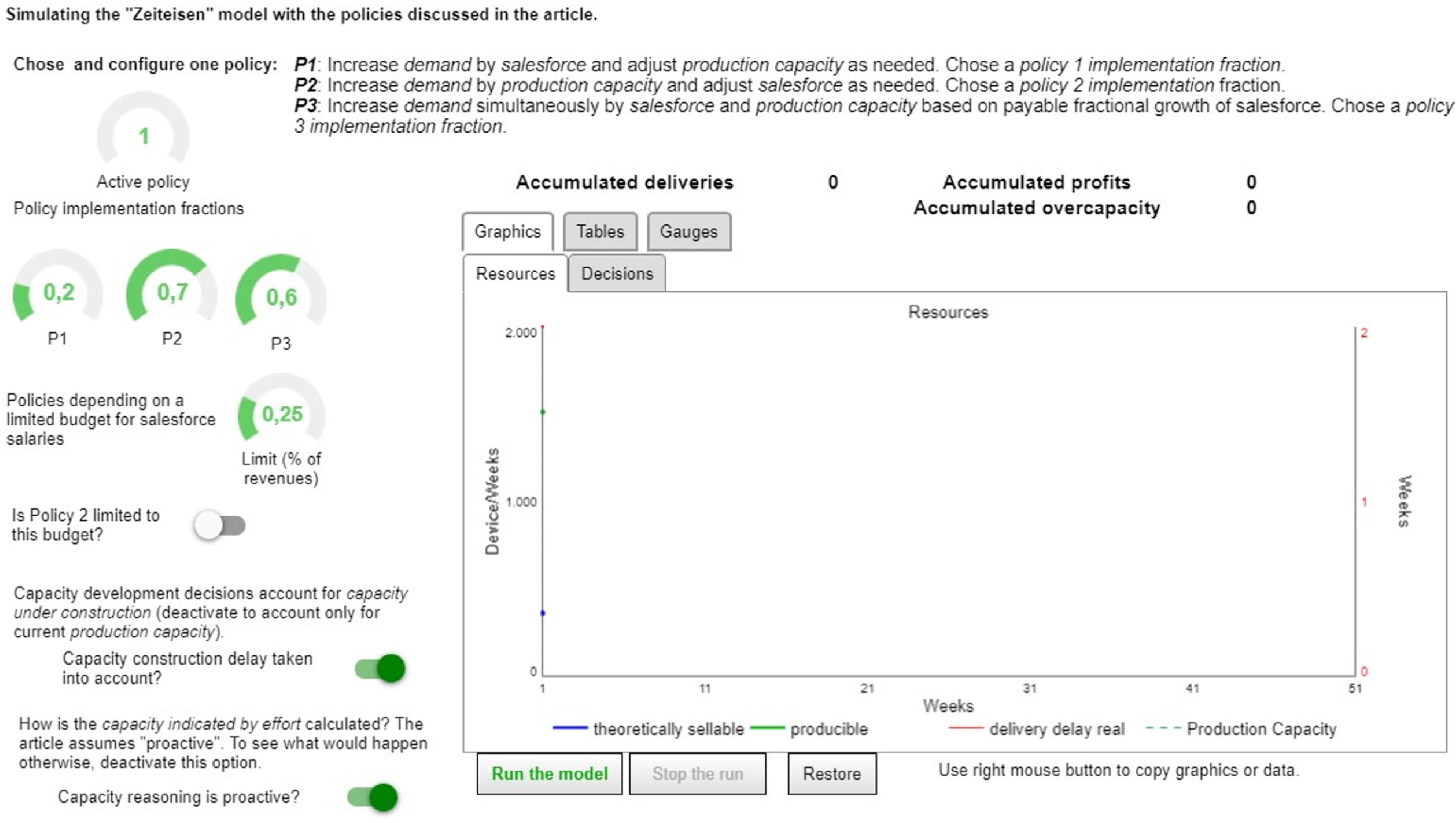
Appendix A. Simulation Model on the INTERNET
The model can be freely accessed and run (without subscription) on the Internet, using any web browser and navigating to the following URL: https://exchange.iseesystems.com/public/martin-schaffernicht/zeiteisen-policies-explorer (accessed on 1 June 2021).
There is only one screen, as shown in the following figure (Figure A1):
Figure A1.
Screen of the user interface of the simulator.

Users can choose which policy to run and set the following parameters:
- Policy implementation fraction: The computed value for the decisions can be used as suggested by the model or at a fraction between 0.1 and 0.9. The main text of the article discusses the behavior assuming one specific policy implementation fraction, but model users can explore how behavior and performance change when a different value is used.
- For policies P1 and P3, the revenue fraction for salesforce salaries can be changed to values smaller than or greater than the default value of 25%. Around 30%, oscillations appear. This is not addressed in the article, but readers may be interested in this aspect.
- For policy P2, one can use the revenue fraction for salesforce salaries to impose an upper limit on recruitments. Table 2 in the article reports on this under the title “P2 limited,” but one can explore the range of effects by varying the control for revenue fraction for salesforce salaries.
- Capacity construction delay accounted for: By default, the computations are based on the total capacity, including the capacity under construction, to avoid the oscillations typical for second order negative feedback loops. This can be deactivated to explore how behaviors change.
- Proactive capacity reasoning: by default, the computations assuming that the degree of change of production capacity is determined proactively. This can be deactivated to explore how behaviors change.
The green “run the model” command button starts an interactive simulation, which then can be stopped by the red “stop the run” button. The “restore” button will reset all parameters to their respective default values and erase the graphics.
Appendix B. Summary Results from All Simulated Policies
The following Table A1 reports the same variables and indicators as Table 2 in the article, but it includes the results for policies P1 and P3 for alternative values of the revenue fraction for salesforce salaries. It is important to consider the production capacity and the accumulation of overcapacity (either too many or too few salespeople compared to production capacity) to interpret the results in terms of accumulated profits. The unit purchasing cost of production capacity is so high that the company cannot recover the initial expenses in the first year. It follows that if more production capacity is built in the first year, accumulated profits will have increasingly negative numbers. Over the life cycle time of the equipment (production capacity), each unit will become profitable provided the company can sell according to production capacity. However, if there is overcapacity, the sales revenues will not recover the initial expenses. This is where P2 does better than P1 and P2, especially when compared to the alternative values of the revenue fraction for salesforce salaries.

Table A1.
Results from simulating the policies with different assumptions concerning the revenue fraction for salesforce salaries.
Table A1.
Results from simulating the policies with different assumptions concerning the revenue fraction for salesforce salaries.
| Indicator | Specific Policy | |||||||
|---|---|---|---|---|---|---|---|---|
| P1 Default | P1 50% | P1 75% | P2 Default | P2 Limited | P3 Default | P3 50% | P3 75% | |
| Parameters | ||||||||
| policy implementation fraction | 0.2 | 0.7 | 0.6 | |||||
| revenue fraction for salesforce salaries | 25% | 50% | 75% | na | 25% | 25% | 50% | 75% |
| Model Variables | ||||||||
| Sales Force | 398 | 11,402 | 29,698 | 12,656 | 398 | 398 | 9435 | 28,200 |
| Theoretically sellable | 3585 | 103,000 | 267,000 | 113,907 | 3585 | 3585 | 84,914 | 253,801 |
| Production Capacity | 5930 | 56,539 | 93,209 | 118,860 | 16,974 | 6200 | 35,744 | 70,105 |
| Production capacity surplus or lack absolute | 2344 | −46,461 | −173,791 | 4952 | 13,388 | 2615 | −49,169 | −183,696 |
| Production capacity surplus or lack relative | 65% | −45% | −65% | 4% | 373% | 73% | −58% | −72% |
| Accumulated deliveries | 66,284 | 585,194 | 921,889 | 823,596 | 66,284 | 66,284 | 724,657 | 1,435,274 |
| Accumulated excess production capacity | 68,859 | 4487 | 3962 | 65,959 | 232,489 | 68,723 | 6164 | 3962 |
| Accumulated excess salesforce | 0 | 469,547 | 1,487,410 | 0 | 0 | 0 | 799,017 | 3,102,219 |
| Delivery delay real | 2.0 | 3.5 | 5.3 | 2.0 | 2.0 | 2.0 | 5.2 | 6.7 |
| Accumulated profits | −126,630,840 | −2,106,130,554 | −4,043,396,613 | −5,700,338,232 | −458,165,449 | −89,220,517 | −798,131,201 | −1,732,646,384 |
| Additional Indicators | ||||||||
| Additional deliveries | 49,004 | 567,914 | 904,609 | 806,316 | 49,004 | 49,004 | 707,377 | 1,417,994 |
| Total growth in % | 284% | 3287% | 5235% | 4666% | 284% | 284% | 4094% | 8206% |
| Monthy growth rate | 9% | 34% | 39% | 38% | 9% | 9% | 36% | 44% |
| Steady state deliveries at end of year | 49,004 | 567,914 | 904,609 | 806,316 | 49,004 | 49,004 | 707,377 | 1,417,994 |
| Accelerating growth | Yes | Yes | Yes | Yes | Yes | Yes | Yes | Yes |
| Behavior smoothness of resources | Continuous | Continuous | Continuous | Continuous | Continuous | Continuous | Continuous | Continuous |
| Strength of growth | Moderate | Extreme | Extreme | Extreme | Moderate | Moderate | Extreme | Extreme |
| Sustainable | Yes | Yes | Yes | Yes | Yes | Yes | Yes | Yes |
| Delivery delay behavior | Steady | Increase | Increase | Steady | Steady | Steady | Increase | Increase |
| Delivery delay values | Constant | Oscillation | Oscillation | Constant | Constant | Constant | Oscillation | Oscillation |
| Likely to be followed | Yes | No | No | Tes | No | Yes | No | No |
Appendix C. Model Documentation
The simulation model has been developed using the STELLA Architect software package. The equations are presented using the following typographical conventions. Stock variables are printed in boldface; the connected flow variables are boldface italic. All other elements are referred to as intermediate variables, including constants. The model is organized in sectors—groupings of variables—and one module (like a sub-model). Inside each sector (and module), the sequence of presentation is stocks, flows, and then intermediate variables in alphabetical order. In total, the model has 8 stocks and 12 flows.
Appendix C.1. Main Model
Appendix C.1.1. Salesforce
Searching(t) = Searching(t − dt) + (to_recruit − recruited) * dt.
INIT Searching = 0.
UNITS: Individual.
DEF: Number of currently searched for salespeople.
USED BY: recruited, relative_SF_gap, total_salesforce.
INFLOW: to_recruit = IF(autopilot_switch = 0) THEN(now_hiring/time_unit) ELSE(recruitment_by_policy/time_unit).
UNITS: Individual/Weeks.
DEF: Weekly decision to search for additional salespeople.
USED BY: net_salesforce_decisions, Searching.
OUTFLOW: recruited = INT (Searching/hiring_delay).
UNITS: Individual/Weeks.
DEF: Weekly actual recruitment of new salespeople.
USED BY: Searching, Sales_Force.
Sales_Force(t) = Sales_Force(t − dt) + (recruited − laid_off) * dt.
INIT Sales_Force = 40.
UNITS: Individual.
DEF: Currently working salespeople.
USED BY: payable_additional_salesforce, orders, salesman_productivity_reported, minimum_delivery_to_pay_current_salesforce, Accounting, relative_SF_gap, expected_sales, total_salesforce, theoretically_sellable, Accounting.salesforce_costs.
INFLOW: recruited = INT(Searching/hiring_delay).
UNITS: Individual/Weeks.
DEF: Weekly actual recruitment of new salespeople.
USED BY: Searching, Sales_Force.
OUTFLOW: laid_off = −now_firing/firing_delay.
UNITS: Individual/Weeks.
DEF: Weekly number of laid off salespeople.
USED BY: net_salesforce_decisions, Sales_Force.
Appendix C.1.2. Production Capacity
Capacity_in_preparation(t) = Capacity_in_preparation(t − dt) + (additional_production_capacity − going_into_service) * dt.
INIT Capacity_in_preparation = 0.
UNITS: Device/Weeks.
DEF: Capacity units being prepared currently.
USED BY: Production_Capacity_considered.
INFLOW: additional_production_capacity = additional_production_capacity_Participant * (autopilot_switch = 0) + capacity_adjustment_by_P1 * (autopilot_switch * Policy = 1) + capacity_adjustment_by_P2 * (autopilot_switch * Policy = 2) + capacity_adjustment_by_P3 * (autopilot_switch * Policy = 3).
UNITS: Device/Weeks/Weeks.
DEF: Additional Capacity units whose preparation is decided per week. If autopilot is off, then the box/slider put a fraction of the investment indicated by effort. If the autopilot is on, then the Policy controls the decision: (1) P1 and P2: investment indicated by effort; (3): P3, additional production capacity P3.
USED BY: going_into_service, Accounting, net_production_capacity_decisions, Accounting.investment_costs, Capacity_in_preparation.
OUTFLOW: going_into_service = DELAY(additional_production_capacity; capacity_installment_delay; 0).
UNITS: Device/Weeks/Weeks.
DEF: Capacity units going on-line per week.
USED BY: Capacity_in_preparation, Production_Capacity.
Production_Capacity(t) = Production_Capacity(t − dt) + (going_into_service − capacity_sold_off) * dt.
INIT Production_Capacity = PC_init.
UNITS: Device/Weeks.
DEF: Weekly number of watches that can be produced at full capacity utilization
USED BY: producible, Potentials, Production_Capacity_considered, Accounting, CUF_indicated, delivery_delay_min, Potentials.PPC_5, Potentials.PPC_6, Potentials.PPC_7, Potentials.PPC_10, Potentials.PPC_12, Potentials.PPC_14, Potentials.PPC_15, Potentials.PPC_18, Potentials.PPC_21, Accounting.capacity_maintenance_costs.
INFLOW: going_into_service = DELAY (additional_production_capacity; capacity_installment_delay; 0).
UNITS: Device/Weeks/Weeks.
DEF: Capacity units going on-line per week.
USED BY: Capacity_in_preparation, Production_Capacity.
OUTFLOW: capacity_sold_off = −disinvestment.
UNITS: Device/Weeks/Weeks.
DEF: Capacity units sold off per week.
USED BY: net_production_capacity_decisions, Production_Capacity.
Appendix C.1.3. Orders
Backlog(t) = Backlog(t − dt) + (orders − deliveries) * dt.
INIT Backlog = 720.
UNITS: Device.
DEF: All orders currently waiting to be produced and delivered.
USED BY: delivery_delay_real, deliveries_max, Potentials, CUF_indicated, delivery_delay_min, desirable_deliveries.
INFLOW: orders = INT(Sales_Force * effect_of_delivery_delay_on_demand * salesman_productivity_max).
UNITS: Device/Weeks.
DEF: Weekly number of new orders.
USED BY: salesman_productivity_reported, Backlog.
OUTFLOW: deliveries = MIN (producible; deliveries_limit).
UNITS: Device/Weeks.
DEF: Weekly number of delivered orders.
USED BY: delivery_delay_real, sales_revenues, Accounting, additonal_deliveries, Accounting.variable_costs, Accounting.unit_production_cost, Accounting.variable_capital_costs, Accounting.variable_worker_costs, Backlog.
Appendix C.1.4. Intermediate Variables
Additional_production_capacity_Participant = IF (Capacity_adjustment_box = 0) THEN (investment_indicated_by_effort * Capacity_adjustment_slider) ELSE (investment_indicated_by_effort * Capacity_adjustment_box)
UNITS: Device/Weeks/Weeks.
DEF: Additional production capacity according to a player.
USED BY: additional_production_capacity.
Additional_salesforce_for_excess_producibility = theoretic_excess_productibility/(0.9 * salesman_productivity_max)
UNITS: Individual.
DEF: Number of additional salespeople that would be needed to sell those watches that can be produced but not sold by the current workforce.
USED BY: recruitment_by_policy, Salesforce_fractional_effort_from_Capacity
additional_SF_monthly_salary_costs = payable_additional_salesforce * salesperson_monthly_salary.
UNITS: Euros/Month.
DEF: Money implied by salaries of the additional salespeople.
autopilot_switch = 1.
UNITS: unitless.
DEF: if set to 1, the model policies regulate the decisins; if set to 0, users take the decisions.
USED BY: deliveries_limit, additional_production_capacity, to_recruit
capacity_adjustment_indicated_by_effort = Capacity_indicated_by_effort-Production_Capacity_considered.
UNITS: Device/Weeks.
DEF: Theoretically indicated additional production capacity units according to the “stress” reasoning. This is the stock’s value, so it cannot directly be used in a flow.
USED BY: investment_indicated_by_effort, disinvestment_indicated_by_effort
Capacity_fractional_effort = (desirable_deliveries/theoretically_productible)/2.
UNITS: unitless.
USED BY: Capacity_indicated_by_effort.
Capacity_adjustment_box = 1.
UNITS: unitless.
DEF: Value of the edit box in the user interface.
USED BY: additional_production_capacity_Participant, disinvestment
Capacity_adjustment_slider = 0.
UNITS: unitless.
DEF: Value of the slider in the user interface.
USED BY: additional_production_capacity_Participant, disinvestment.
Capacity_indicated_by_effort = Production_Capacity_considered * (proactiveness + Capacity_fractional_effort).
UNITS: Device/Weeks.
USED BY: capacity_adjustment_indicated_by_effort.
capacity_installment_delay = 8
UNITS: Weeks.
USED BY: going_into_service.
Capacity_Utilization_Fraction = Shifts_per_week/Shifts_per_week_max.
UNITS: unitless.
USED BY: producible, theoretically_productible.
Days_per_week = 7.
UNITS: days/week.
USED BY: Shifts_per_week.
delay_perceived = 1.
UNITS: unitless.
DEF: Allows to simulate according to if the decision-maker takes the capacity installment delay into account (=1, default) or not (=0: like in the literature).
USED BY: Production_Capacity_considered.
delay_perception_time = 6.
UNITS: Weeks.
USED BY: delivery_delay_perceived.
deliveries_limit = INT (deliveries_max/(1 + autopilot_switch))
UNITS: Device/Weeks.
USED BY: deliveries.
delivery_delay_perceived = SMTH1 (delivery_delay_real; delay_perception_time; delivery_delay_real).
UNITS: Weeks.
DEF: The clients’ expectation regarding the delivery delay, which adjusts progressively to the actual delivery delay.
USED BY: effect_of_delivery_delay_on_demand.
delivery_delay_real = SAFEDIV(Backlog; deliveries).
UNITS: Weeks.
DEF: Actual number of weeks it takes between order and delivery.
USED BY: delivery_delay_perceived, reported_delivery_delay disinvestment = IF (Capacity_adjustment_box = 0) THEN (disinvestment_indicated_by_effort * Capacity_adjustment_slider) ELSE (disinvestment_indicated_by_effort * Capacity_adjustment_box).
UNITS: Device/Weeks/Weeks.
USED BY: capacity_sold_off.
Disinvestment_indicated_by_effort = MIN(0; capacity_adjustment_indicated_by_effort)/time_unit.
UNITS: Device/Weeks/Weeks.
DEF: Theoretically indicated excess production capacity units according to the “stress” reasoning. Adjusted to time units to fit as flow variable.
USED BY: disinvestment.
effect_of_delivery_delay_on_demand = GRAPH(delivery_delay_perceived).
| Input | Output |
| 0 | 1.000 |
| 1 | 0.970 |
| 2 | 0.900 |
| 3 | 0.730 |
| 4 | 0.530 |
| 5 | 0.380 |
| 6 | 0.250 |
| 7 | 0.150 |
| 8 | 0.080 |
| 9 | 0.030 |
| 10 | 0.020 |
UNITS: unitless.
DEF: Effect of the expectation regarding the delivery delay on the willingness to buy.
USED BY: orders.
expected_sales_revenues = SMTH1(sales_revenues; revenue_averaging_time; sales_revenues).
UNITS: Euros/Weeks.
DEF: The expected sales revenues are a moving average of the past weeks.
USED BY: payable_salesforce, budget_for_salesforce_costs.
firing_delay = 1.
UNITS: Weeks.
DEF: Time it takes to implement layoff decisions.
USED BY: laid_off.
hiring_delay = 1 + relative_SF_gap * (hiring_delay_max-hiring_delay_min)
UNITS: Weeks.
DEF: Time it takes to find and recruit the number of additional salespeople sought for. Depends on the relationship of the number of searched salespeople to the current salesforce.
USED BY: recruited.
hiring_delay_max = 4.
UNITS: Weeks.
DEF: Longest possible time to find and recruit additional salespeople.
USED BY: hiring_delay.
hiring_delay_min = 1.
UNITS: Weeks.
DEF: Shortest possible time to find and recruit additional salespeople.
USED BY: hiring_delay.
Investment_indicated_by_effort = MAX(capacity_adjustment_indicated_by_effort; 0)/time_unit.
UNITS: Device/Weeks/Weeks.
DEF: Theoretically indicated additional production capacity units according to the “stress” reasoning. Adjusted to time units to fit as flow variable.
USED BY: additional_production_capacity_Participant, capacity_adjustment_by_P1, capacity_adjustment_by_P2, additional_capacity_investment_costs.
Sales_force_box = 1.
UNITS: unitless.
DEF: Value of the edit box in the user interface.
USED BY: now_hiring_C, now_firing_C.
Sales_force_slider = 0
UNITS: unitless.
DEF: Value of the slider in the user interface.
USED BY: now_hiring_E, now_firing_E.
recruitment_by_policy = IF(Policy = 2) THEN(additional_salesforce_for_excess_producibility) ELSE(payable_additional_salesforce).
UNITS: Individual.
DEF: Weekly number of salespeople to be searched and recruited according to one pf the policies implemented in the model. If it is policy P2, then hiring is driven by the additional salesforce for excess producibility, otherwise it is driven by payable additional salesforce.
USED BY: to_recruit.
Now_firing = IF(now_firing_C=0) THEN(now_firing_E) ELSE(now_firing_C)
UNITS: Individual.
USED BY: laid_off.
Now_firing_C = INT(Sales_force_box * MIN(0; payable_additional_salesforce)).
UNITS: Individual.
USED BY: now_firing.
Now_firing_E = INT(Sales_force_slider * MIN(0; payable_additional_salesforce)).
UNITS: Individual.
USED BY: now_firing.
Now_hiring = IF(now_hiring_C = 0) THEN(now_hiring_E) ELSE(now_hiring_C).
UNITS: Individual.
DEF: Weekly number of salespeople to be searched and recruited according to a player.
USED BY: to_recruit.
Now_hiring_C = INT(Sales_force_box * MAX(payable_additional_salesforce; 0))
UNITS: Individual.
DEF: Weekly number of salespeople to be searched and recruited according to a player if the user interface has an edit box as control.
USED BY: now_hiring.
Now_hiring_E = INT(Sales_force_slider * MAX(payable_additional_salesforce; 0))
UNITS: Individual.
DEF: Weekly number of salespeople to be searched and recruited according to a player if the user interface has a slider as control.
USED BY: now_hiring.
Payable_additional_salesforce = payable_salesforce-Sales_Force.
UNITS: Individual.
DEF: Number of additional salespeoplpe which can be paid, accounting for the currently searched salespeople (to avoid oscillations).
USED BY: recruitment_by_policy, now_hiring_E, now_hiring_C, now_firing_C, now_firing_E, additional_SF_monthly_salary_costs, sales_force_growth_rate, Salesforce_fractional_effort_from_budget.
payable_salesforce = INT((revenue_fraction_for_salesforce_salaries * expected_sales_revenues)/(salesperson_monthly_salary/weeks_per_month))
UNITS: Individual.
DEF: Payable number pf salespeople according to the salaries and the expected sales revenues, assuming a stable fraction.
USED BY: payable_additional_salesforce, Potentials, Potentials.payable_sales
PC_init = 1512.
UNITS: Device/Weeks.
DEF: 1512.
proactiveness = 1.
UNITS: unitless.
DEF: Used to determine capacity indicated by effort, which can be in a reactive mode to replicate results from Forrester and from Morecroft, or in a proactive mode to drive, for instance, the weightlifter.
USED BY: Capacity_indicated_by_effort.
producible = INT(Capacity_Utilization_Fraction * Production_Capacity).
UNITS: Device/Weeks.
USED BY: deliveries.
Production_Capacity_considered = delay_perceived * Capacity_in_preparation+Production_Capacity.
UNITS: Device/Weeks.
USED BY: theoretically_productible, Capacity_indicated_by_effort, capacity_adjustment_indicated_by_effort, capacity_adjustment_by_P3, Capacity_indicated_by_delay_gap, capacity_adjustment_indicated_by_delay_gap.
relative_SF_gap = Searching/Sales_Force.
UNITS: unitless.
DEF: The relationship of the number of searched salespeople to the current salesforce.
USED BY: hiring_delay.
revenue_averaging_time = 3.
UNITS: Weeks.
DEF: Number of weeks in the moving average for sales values expected.
USED BY: expected_sales_revenues.
revenue_fraction_for_salesforce_salaries = 0.25.
UNITS: unitless.
DEF: Percentage of the expected sales revenues which can be used for paying salesforce salaries. In the original mode = 0.1. Under the price and salary assumptions of the revised model, it has to be at least 19.5% (initialization equilibrium). If = 25%, the default situation generates the possibility to pay 51 salespeople, therefore there is space to hire additional salesforce.
USED BY: payable_salesforce, budget_for_salesforce_costs.
Sales_revenues = deliveries * unit_sales_price.
UNITS: Euros/Weeks.
DEF: Amount received for the watches delivered weekly.
USED BY: expected_sales_revenues, Accounting, Accounting.total_revenues.
Salesman_productivity_max = 10.
UNITS: Device/Weeks/Individual.
DEF: Highest theoretical number of weekly new orders one salesperson can achieve.
USED BY: orders, minimum_delivery_to_pay_current_salesforce, expected_sales, salesforce_costs_per_watch, theoretically_sellable, additional_salesforce_for_excess_producibility.
Salesperson_monthly_salary = 3000.
UNITS: Euros/Month/Individual.
DEF: Monthly salary for each of the salespeople.
USED BY: payable_salesforce, Accounting, additional_SF_monthly_salary_costs, salesforce_costs_per_watch, Accounting.salesforce_costs.
Shifts_per_day = 3.
UNITS: shifts/days.
USED BY: Shifts_per_week.
Shifts_per_week = Days_per_week * Shifts_per_day.
UNITS: shifts/week.
USED BY: Capacity_Utilization_Fraction, Accounting, Accounting.extra_shifts_multiplier.
Shifts_per_week_max = 21.
UNITS: shifts/week.
USED BY: Capacity_Utilization_Fraction.
theoretic_excess_productibility = MAX(theoretically_productible-theoretically_sellable; 0).
UNITS: Device/Weeks.
DEF: Weekly number of producible watches that would not be sold with the current salesforce.
USED BY: additional_salesforce_for_excess_producibility.
Theoretically_productible = Capacity_Utilization_Fraction * Production_Capacity_considered
UNITS: Device/Weeks.
DEF: Weekly number of producible watches according to the considered production capacity and the capacity utilization fraction.
USED BY: Capacity_fractional_effort, theoretic_excess_productibility
theoretically_sellable = Sales_Force * 0.9 * salesman_productivity_max
UNITS: Device/Weeks.
DEF: Weekly number of new orders which the salesforce could achieve at the maximum productivity.
USED BY: theoretic_excess_productibility.
unit_sales_price = 431.
UNITS: Euros/Device.
DEF: Amount paid by clients per watch.
USED BY: sales_revenues.
weeks_per_month = 4.
UNITS: Weeks/Month.
DEF: Each month is assumed to last exactly 4 weeks.
USED BY: payable_salesforce, Accounting, salesforce_costs_per_watch, Accounting.salesforce_costs.
Appendix C.2. Policy GP1
capacity_adjustment_by_P1 = (investment_indicated_by_effort * Policy_1_by_effort + capacity_adjustment_indicated_by_delay_gap * (1 - Policy_1_by_effort)) * P1_fraction.
UNITS: Device/Weeks/Weeks.
USED BY: additional_production_capacity.
capacity_adjustment_indicated_by_delay_gap = (Capacity_indicated_by_delay_gap-Production_Capacity_considered)/time_unit.
UNITS: Device/Weeks/Weeks.
USED BY: capacity_adjustment_by_P1.
Capacity_indicated_by_delay_gap = delivery_delay_gap_relative * Production_Capacity_considered.
UNITS: Device/Weeks.
USED BY: capacity_adjustment_indicated_by_delay_gap.
delivery_delay_gap = reported_delivery_delay-desired_delivery_delay.
UNITS: Weeks.
USED BY: delivery_delay_gap_relative.
Delivery_delay_gap_relative = delivery_delay_gap/desired_delivery_delay.
UNITS: unitless.
USED BY: Capacity_indicated_by_delay_gap.
Delivery_delay_reporting_time = 4.
UNITS: Weeks.
USED BY: reported_delivery_delay.
P1_fraction = 1.
UNITS: unitless.
USED BY: capacity_adjustment_by_P1.
Policy_1_by_effort = 1.
UNITS: unitless.
DEF: 1: depending on the effort logic.
0: reactive, depending on the delay gap.
USED BY: capacity_adjustment_by_P1.
reported_delivery_delay = SMTH1(delivery_delay_real; delivery_delay_reporting_time; delivery_delay_real).
UNITS: Weeks.
USED BY: DD_underrun, delivery_delay_gap.
Appendix C.3. Policy GP2
capacity_adjustment_by_P2 = P2_fraction * investment_indicated_by_effort.
UNITS: Device/Weeks/Weeks.
USED BY: additional_production_capacity.
P2_fraction = 1.
UNITS: unitless.
USED BY: capacity_adjustment_by_P2.
Appendix C.4. Policy GP3
capacity_adjustment_by_P3 = (sales_force_growth_rate * P3a_fraction) * Production_Capacity_considered/time_unit.
UNITS: Device/Weeks/Weeks.
DEF: In salesforce changes X%, so shall the production capacity.
USED BY: additional_production_capacity.
P3a_fraction = 1.
UNITS: unitless.
USED BY: capacity_adjustment_by_P3.
sales_force_growth_rate = payable_additional_salesforce/total_salesforce.
UNITS: unitless.
USED BY: capacity_adjustment_by_P3.
Appendix C.5. Stress_on_Salesforce
Salesforce_fractional_effort_from_budget = SAFEDIV(payable_additional_salesforce; total_salesforce; 0).
UNITS: unitless.
DEF: Fraction of the salary costs for the additonal required salesforce as compared to the salary costs of the current total salesforce.
This was one option for representing the stress on the salesforce resource, but it is currently not used.
Salesforce_fractional_effort_from_Capacity = SAFEDIV(additional_salesforce_for_excess_producibility; total_salesforce; 0)
UNITS: unitless
DEF: Fraction of additional salespeople which would be required as compared to the current total salesforce. This is not used in the model’s computations, but fed to the user (human decision-maker) on the user interface.
total_salesforce = Sales_Force+Searching.
UNITS: Individual.
USED BY: Salesforce_fractional_effort_from_Capacity, sales_force_growth_rate, Salesforce_fractional_effort_from_budget.
Appendix C.6. Auxiliary_Calculations
Accumulated_DD_underrun(t) = Accumulated_DD_underrun(t − dt) + (DD_underrun) * dt.
INIT Accumulated_DD_underrun = 0.
UNITS: Weeks.
INFLOW: DD_underrun = MAX(2-reported_delivery_delay; 0)/time_unit.
UNITS: unitless.
USED BY: Accumulated_DD_underrun.
Accumulated_deliveries(t) = Accumulated_deliveries(tt − dt) + (additonal_deliveries) * dt
INIT Accumulated_deliveries = 0.
UNITS: Device.
INFLOW: additonal_deliveries = deliveries.
UNITS: Device/Weeks.
USED BY: Accumulated_deliveries.
additional_capacity_investment_costs = investment_indicated_by_effort * Accounting.investiment_cost_of_capacity_unit
UNITS: Euros.
CUF_indicated = ((Backlog/2)/time_unit)/Production_Capacity.
UNITS: unitless.
Current_week = TIME.
UNITS: Weeks.
USED BY: Game_on.
deliveries_max = Backlog/time_unit.
UNITS: Device/Weeks.
USED BY: deliveries_limit.
delivery_delay_min = Backlog/Production_Capacity.
UNITS: Weeks.
desirable_deliveries = Backlog/desired_delivery_delay.
UNITS: Device/Weeks.
DEF: The weekly deliveries which are just enough to keep the delivery delay equal to the desired delivery delay.
USED BY: Capacity_fractional_eff.ort.
desired_delivery_delay = 2.
UNITS: Weeks.
DEF: The goal: 2 weeks.
USED BY: desirable_deliveries, delivery_delay_gap, delivery_delay_gap_relative
expected_sales = Sales_Force * salesman_productivity_max * 0.9
UNITS: Device/Weeks.
Game_on = 51-Current_week.
UNITS: Weeks.
minimum_delivery_to_pay_current_salesforce = (salesman_productivity_max * 0.85) * Sales_Force.
UNITS: Device/Weeks.
net_production_capacity_decisions = additional_production_capacity-capacity_sold_off.
UNITS: Device/Weeks/Weeks.
net_salesforce_decisions = to_recruit-laid_off.
UNITS: Individual/Weeks.
salesman_productivity_reported = orders/Sales_Force.
UNITS: Device/Weeks/Individual.
time_unit = 1.
UNITS: Weeks.
USED BY: CUF_indicated, deliveries_max, DD_underrun, to_recruit, disinvestment_indicated_by_effort, capacity_adjustment_by_P3, investment_indicated_by_effort, capacity_adjustment_indicated_by_delay_gap.
Appendix C.7. Accounting Module
Accounting.Accumulated_profits(t) = Accumulated_profits(tt − dt) + (weekly_profits) * dt.
INIT Accounting.Accumulated_profits = 0.
UNITS: Euros.
INFLOWS: accounting.weekly_profits = total_revenues-total_costs.
UNITS: Euros/Weeks.
USED BY: Accounting.Accumulated_profits.
Accounting.capacity_maintenance_costs = Production_Capacity * maintenance_costs_per_capacity_unit.
UNITS: Euros/Weeks.
USED BY: Accounting.total_costs, Accounting.total_production_costs.
Accounting.capacity_sold_off = 0.
UNITS: Device/Weeks/Weeks.
USED BY: Accounting.sell_off_revenue.
Accounting.effective_variable_cost_per_unit = (1-labor_cost_fraction) * variable_costs_per_unit + labor_costs_per_unit.
UNITS: Euros/Device.
USED BY: Accounting.variable_costs.
Accounting.extra_shifts_multiplier = GRAPH(.Shifts_per_week).
| Input | Output |
| 0 | 0.0000 |
| 1 | 0.0000 |
| 2 | 0.0000 |
| 3 | 0.0000 |
| 4 | 0.0000 |
| 5 | 1.0000 |
| 6 | 1.041666667 |
| 7 | 1.107142857 |
| 8 | 0.0000 |
| 9 | 0.0000 |
| 10 | 1.1250 |
| 11 | 0.0000 |
| 12 | 1.1666666667 |
| 13 | 0.0000 |
| 14 | 1.232142857 |
| 15 | 1.2500 |
| 16 | 0.0000 |
| 17 | 0.0000 |
| 18 | 1.291666667 |
| 19 | 0.0000 |
| 20 | 0.0000 |
| 21 | 1.357142857 |
UNITS: unitless.
USED BY: Accounting.labor_costs_per_unit.
Accounting.investiment_cost_of_capacity_unit = 20,000.
UNITS: Euros/(Device/Weeks).
USED BY: Accounting.investment_costs, Accounting.sell_off_price_per_unit, additional_capacity_investment_costs, capacity_cost_per_watch, additional_production_capacity_P3_b.
Accounting.investment_costs = additional_production_capacity * investiment_cost_of_capacity_unit.
UNITS: Euros/Weeks.
USED BY: Accounting.total_costs.
Accounting.labor_cost_fraction = 0.7
UNITS: unitless.
USED BY: Accounting.labor_cost_per_unit_normal, Accounting.effective_variable_cost_per_unit, Accounting.variable_capital_costs.
Accounting.labor_cost_per_unit_normal = labor_cost_fraction * variable_costs_per_unit.
UNITS: Euros/Device.
USED BY: Accounting.labor_costs_per_unit
Accounting.labor_costs = variable_worker_costs+salesforce_costs
UNITS: Euros/Weeks.
Accounting.labor_costs_per_unit = labor_cost_per_unit_normal * extra_shifts_multiplier
UNITS: Euros/Device.
USED BY: Accounting.effective_variable_cost_per_unit, Accounting.variable_worker_costs.
Accounting.maintenance_costs_per_capacity_unit = 0.
UNITS: Euros/Device.
DEF: Was originally set to 48. Put to 0 on December 4 2019 because of an unclear computation error.
USED BY: Accounting.capacity_maintenance_costs
Accounting.salesforce_costs = salesperson_monthly_salary/weeks_per_month *.Sales_Force
UNITS: Euros/Weeks
USED BY: Accounting.total_costs, Accounting.labor_costs
Accounting.sell_off_discount_fraction = 0.5.
UNITS: unitless.
USED BY: Accounting.sell_off_price_per_unit.
Accounting.sell_off_price_per_unit = (1-sell_off_discount_fraction) * investiment_cost_of_capacity_unit.
UNITS: Euros/(Device/Weeks).
USED BY: Accounting.sell_off_revenue.
Accounting.sell_off_revenue = capacity_sold_off * sell_off_price_per_unit.
UNITS: Euros/Weeks.
USED BY: Accounting.total_revenues.
Accounting.total_costs = investment_costs + capacity_maintenance_costs + variable_costs + salesforce_costs.
UNITS: Euros/Weeks.
USED BY: Accounting.weekly_profits.
Accounting.total_production_costs = variable_costs+capacity_maintenance_costs.
UNITS: Euros/Weeks.
USED BY: Accounting.unit_production_cost.
Accounting.total_revenues = sales_revenues+sell_off_revenue.
UNITS: Euros/Weeks.
USED BY: Accounting.weekly_profits.
Accounting.unit_production_cost = SAFEDIV(total_production_costs; deliveries).
UNITS: Euros/Device.
Accounting.variable_capital_costs = deliveries * ((1-labor_cost_fraction) * variable_costs_per_unit).
UNITS: Euros/Weeks.
Accounting.variable_costs = deliveries * effective_variable_cost_per_unit.
UNITS: Euros/Weeks.
USED BY: Accounting.total_costs, Accounting.total_production_costs.
Accounting.variable_costs_per_unit = 200.
UNITS: Euros/Device.
USED BY: Accounting.labor_cost_per_unit_normal, Accounting.effective_variable_cost_per_unit, Accounting.variable_capital_costs.
Accounting.variable_worker_costs = .deliveries * labor_costs_per_unit.
UNITS: Euros/Weeks.
USED BY: Accounting.labor_costs.
References
- Barney, J. Firm Resources and Sustained Competitive Advantage. J. Manag. 1991, 17, 99–120. [Google Scholar] [CrossRef]
- Crook, T.R.; Ketchen, D.J.; Combs, J.G.; Todd, S.Y. Strategic resources and performance: A meta-analysis. Strateg. Manag. J. 2008, 29, 1141–1154. [Google Scholar] [CrossRef]
- Kor, Y.Y.; Mahoney, J.T. Edith Penrose’s (1959) Contributions to the Resource-based View of Strategic Management. J. Manag. Stud. 2004, 41, 11. [Google Scholar] [CrossRef]
- Penrose, E.T. The Theory of the Growth of the Firm; John Wiley: New York, NY, USA, 1959. [Google Scholar]
- Peteralf, M.A. The Cornerstones of Competitive Advantage: A Resource-Based View. Strateg. Manag. J. 1993, 14, 12. [Google Scholar]
- Wernerfelt, B. A Resource-Based view of the Firm. Strateg. Manag. J. 1984, 5, 10. [Google Scholar] [CrossRef]
- Warren, K. Improving strategic management with the fundamental principles of system dynamics. Syst. Dyn. Rev. 2005, 21, 329–350. [Google Scholar] [CrossRef]
- Barney, J. Is the Resource-Based “View” a Useful Perspective for Strategic Management Research? Yes. Acad. Manag. Rev. 2001, 26, 41–56. [Google Scholar]
- Kunc, M.H.; Morecroft, J.D.W. Managerial decision making and firm performance under a resource-based paradigm. Strateg. Manag. J. 2010, 31, 1164–1182. [Google Scholar] [CrossRef]
- Priem, R.L.; Butler, J.E. Is the Resource-Based “View” a Useful Perspective for Strategic Management Research? Acad. Manag. Rev. 2001, 26, 19. [Google Scholar]
- Ozgun, O.; Barlas, Y. Effects of systemic complexity factors on task difficulty in a stock management game. Syst. Dyn. Rev. 2015, 31, 115–146. [Google Scholar] [CrossRef]
- Moxnes, E. Not only the tragedy of the commons: Misperceptions of feedback and policies for sustainable development. Syst. Dyn. Rev. 2000, 16, 325–348. [Google Scholar] [CrossRef]
- Moxnes, E. Misperceptions of basic dynamics: The case of renewable resource management. Syst. Dyn. Rev. 2004, 20, 139–162. [Google Scholar] [CrossRef]
- Sterman, J. Misperceptions of Feedback in Dynamic Decision Making. Organ. Behav. Hum. Decis. Process. 1989, 43, 301–335. [Google Scholar] [CrossRef] [Green Version]
- Sterman, J. Modeling managerial behavior—Misperceptions of feedback in a dynamic decision-making experiment. Manag. Sci. 1989, 35, 18. [Google Scholar] [CrossRef] [Green Version]
- Baghaei Lakeh, A.; Ghaffarzadegan, N. Does analytical thinking improve understanding of accumulation? Syst. Dyn. Rev. 2015, 31, 46–65. [Google Scholar] [CrossRef]
- Cronin, M.A.; Gonzalez, C. Understanding the building blocks of dynamic systems. Syst. Dyn. Rev. 2007, 23, 1–17. [Google Scholar] [CrossRef]
- Cronin, M.A.; Gonzalez, C.; Sterman, J.D. Why don’t well-educated adults understand accumulation? A challenge to researchers, educators, and citizens. Organ. Behav. Hum. Decis. Process. 2009, 108, 116–130. [Google Scholar] [CrossRef]
- Gonzalez, C.; Wong, H.-y. Understanding stocks and flows through analogy. Syst. Dyn. Rev. 2012, 28, 3–27. [Google Scholar] [CrossRef]
- Sterman, J. Does formal system dynamics training improve people’s understanding of accumulation? Syst. Dyn. Rev. 2010, 26, 316–334. [Google Scholar] [CrossRef] [Green Version]
- Stouten, H.; Grosler, A. Task Complexity in Individual Stock Control Tasks for Laboratory Experiments on Human Understanding of Dynamic Systems. Syst. Res. Behav. Sci. 2017, 34, 62–77. [Google Scholar] [CrossRef]
- Sweeney, L.B.; Sterman, J. Bathtub dynamics: Initial results of a systems thinking inventory. Syst. Dyn. Rev. 2000, 16, 249–286. [Google Scholar] [CrossRef] [Green Version]
- Paich, M.; Sterman, J. Boom, Bust, and Failures to Learn in Experimental Markets. Manag. Sci. 1993, 39, 1439–1458. [Google Scholar] [CrossRef] [Green Version]
- Arquitt, S.; Honggang, X.; Johnstone, R. A system dynamics analysis of boom and bust in the shrimp aquaculture industry. Syst. Dyn. Rev. 2005, 21, 305–324. [Google Scholar] [CrossRef]
- Ford, A. Boom & Bust in Power Plant Construction: Lessons from the California Electricity Crisis. J. Ind. Compet. Trade 2002, 2, 59–74. [Google Scholar]
- Gary, M.S.; Dosi, G.; Lovallo, D. Boom and Bust Behavior: On the Persistence of Strategic Decision Biases. In The Oxford Handbook of Organizational Decision Making; Hodgkinson, G., Starbuck, W., Eds.; Oxford University Press: Oxford, UK, 2008; pp. 33–55. [Google Scholar]
- Morecroft, J.D.W. System Dynamics, RBV and Behavioural Theories of Firm Performance: Lessons from People Express. In Proceedings of the 28th International Conference of the System Dynamics Society, Athens, Greece, 20–24 July 2008; System Dynamics Society: Albany, NY, USA. [Google Scholar]
- Ghaffarzadegan, N.; Lyneis, J.; Richardson, G.P. How small system dynamics models can help the public policy process. Syst. Dyn. Rev. 2011, 27, 22–44. [Google Scholar] [CrossRef] [Green Version]
- Saysel, A.K.; Barlas, Y. Model simplification and validation with indirect structure validity tests. Syst. Dyn. Rev. 2006, 22, 241–262. [Google Scholar] [CrossRef]
- Schoenenberger, L.; Schmid, A.; Ansah, J.; Schwaninger, M. The challenge of model complexity: Improving the interpretation of large causal models through variety filters. Syst. Dyn. Rev. 2017, 33, 112–137. [Google Scholar] [CrossRef]
- Sian Morgan, J.; Graber-Naidich, A. Small system dynamics model for alleviating the general practitioners rural care gap in Ontario, Canada. Socio Econ. Plan. Sci. 2019, 66, 10–23. [Google Scholar] [CrossRef]
- Gonzalez, C.; Fakhari, P.; Busemeyer, J. Dynamic Decision Making: Learning Processes and New Research Directions. Hum. Factors 2017, 59, 713–721. [Google Scholar] [CrossRef] [Green Version]
- Beckmann, J.F.; Birney, D.P.; Goode, N. Beyond Psychometrics: The Difference between Difficult Problem Solving and Complex Problem Solving. Front. Psychol. 2017, 8, 1739. [Google Scholar] [CrossRef] [Green Version]
- Dorner, D.; Funke, J. Complex Problem Solving: What It Is and What It Is Not. Front Psychol. 2017, 8, 1153. [Google Scholar] [CrossRef] [PubMed]
- Qi, L.; Gonzalez, C. Mathematical knowledge is related to understanding stocks and flows: Results from two nations. Syst. Dyn. Rev. 2015, 31, 97–114. [Google Scholar] [CrossRef]
- Sweeny, L.B.; Sterman, J. Cloudy skies: Assessing public understanding of global warming. Syst. Dyn. Rev. 2005, 18, 207–240. [Google Scholar]
- Gary, M.S.; Wood, R.E. Unpacking mental models through laboratory experiments. Syst. Dyn. Rev. 2016, 32, 101–129. [Google Scholar] [CrossRef]
- Warren, K. Competitive Strategy Dynamics; John Wiley & Sons: Chichester, UK, 2008. [Google Scholar]
- Forrester, J.W. Market Growth as Influenced by Capital Investment. Ind. Manag. Rev. 1975, 9, 23. [Google Scholar]
- Morecroft, J.D. Strategic Modelling and Business Dynamics; John Wiley & Sons: Chichester, UK, 2015. [Google Scholar]
- Oliva, R.; Sterman, J.D.; Giese, M. Limits to growth in the new economy: Exploring the “Get Big Fast” strategy in e-commerce. Syst. Dyn. Rev. 2003, 19, 83–117. [Google Scholar] [CrossRef]
- Sterman, J.D.; Henderson, R.; Beinhocker, E.D.; Newman, L.I. Getting Big Too Fast: Strategic Dynamics with Increasing Returns and Bounded Rationality. Manag. Sci. 2007, 53, 683–696. [Google Scholar] [CrossRef]
- Arango, S.; Larsen, E. Cycles in deregulated electricity markets: Empirical evidence from two decades. Energy Policy 2011, 39, 9. [Google Scholar] [CrossRef]
- Schaffernicht, M.F. Causal loop diagrams as means to improve the understanding of dynamic problems: A critical analysis. Syst. Res. Behav. Sci. 2010, 27, 13. [Google Scholar]
- Sterman, J. Business Dynamics—Systems Thinking and Modelling for a Complex World; McGraw Hill: New York, NY, USA, 2000. [Google Scholar]
- Groesser, S.N.; Schaffernicht, M.F. Mental models of dynamic systems: Taking stock and looking ahead. Syst. Dyn. Rev. 2012, 28, 22. [Google Scholar] [CrossRef] [Green Version]
- Sweeney, L.B.; Sterman, J. Thinking about systems: Student and teacher conceptions of natural and social systems. Syst. Dyn. Rev. 2007, 23, 285–312. [Google Scholar] [CrossRef]
- Rahmandad, H.; Repenning, N.; Sterman, J. Effects of feedback delay on learning. Syst. Dyn. Rev. 2009, 25, 309–338. [Google Scholar] [CrossRef]
- Arango, A.S.; Castañeda, A.J.A.; Olaya, M.Y. Laboratory experiments in the system dynamics field. Syst. Dyn. Rev. 2012, 28, 94–106. [Google Scholar] [CrossRef]
- Byrne, R.M.J.; Johnson-Laird, P.N. If and or: Real and counterfactual possibilities in their truth and probability. J. Exp. Psychol. Learn. Mem. Cogn. 2020, 46, 760–780. [Google Scholar] [CrossRef]
- Johnson-Laird, P.N. Mental Models Towards a Cognitive Science of Language; Cambridge University Press: Cambridge, UK, 1983. [Google Scholar]
- Johnson-Laird, P.N.; Byrne, R.M.J. Conditionals: A theory of meaning, pragmatics, and inference. Psychol. Rev. 2002, 109, 646–678. [Google Scholar] [CrossRef] [PubMed]
- Ragni, M.; Johnson-Laird, P. Reasoning about epistemic possibilities. Acta Psychol. 2020, 208. [Google Scholar] [CrossRef]
- Langan-Fox, J.; Anglim, J.; Wilson, J.R. Mental Models, Team Mental Models, and Performance: Process, Development, and Future Directions. Hum. Factors Ergon. Manuf. 2004, 14, 21. [Google Scholar] [CrossRef] [Green Version]
- Mohammed, S.; Klimoski, R.; Rentsch, J.R. The Measurement of Team Mental Models: We Have No Shared Schema. Organ. Res. Methods 2000, 3, 123–165. [Google Scholar] [CrossRef]
- Schaffernicht, M.F. Causal attributions of vineyard executives—A mental model study of vineyard management. Wine Econ. Policy 2017, 6, 107–135. [Google Scholar] [CrossRef]
- Schaffernicht, M.F. Unrecognized interdependencies in mental models—The case for taking feedback loops into account. Syst. Res. Behav. Sci. 2019, 36, 580–603. [Google Scholar] [CrossRef]
- Johnson-Laird, P.N. Mental models and human reasoning. Proc. Natl. Acad. Sci. USA 2010, 107, 18243–18250. [Google Scholar] [CrossRef] [PubMed] [Green Version]
- Wolstenholme, E. Using generic system archetypes to support thinking and modelling. Syst. Dyn. Rev. 2004, 20, 341–356. [Google Scholar] [CrossRef]
- Damasio, A. The Strange Order of Things; Vintage Books: New York, NY, USA, 2018. [Google Scholar]
- Richardson, G.P. Feedback Thought in Social Science and Systems Theory; University of Pennsylvania Press: Philadelphia, PA, USA, 1991. [Google Scholar]
- Viru, A. Early contributions of Russian stress sand exercise physiologists. J. Appl. Physiol. 2002, 92, 1378–1382. [Google Scholar] [CrossRef] [PubMed] [Green Version]
- McEwen, B.S. Central Role of the Brain in Stress and Adaptation: Allostasis, Biological Embedding, and Cumulative Change. In Stress: Concepts, Cognition, Emotion, and Behavior; Fink, G., Ed.; Academic Press: Cambridge, MA, USA, 2016; pp. 39–55. [Google Scholar]
Figure 1.
The fundamental structure of the system with two critical internal resources.

Figure 2.
Salesforce drives demand and production capacity is adjusted.

Figure 3.
Production capacity drives demand and salesforce is adjusted.

Figure 4.
Salesforce and production capacity simultaneously drive demand.

Figure 5.
Salesforce, production capacity, and delivery delay in the classical example from the “market growth model” [39,40].

Figure 6.
Behavior of the “market growth” model without the “eroding goals” loop and with full capacity investment allowance.
Figure 6.
Behavior of the “market growth” model without the “eroding goals” loop and with full capacity investment allowance.

Figure 7.
The behavior of the resources under policy P1.

Figure 8.
Adjusting the salesforce and the production capacity under policy P1.

Figure 9.
The behavior of the resources under policy P2.

Figure 10.
The behavior of the resources under policy P3.

Figure 11.
Adjusting the salesforce and the production capacity under policy P3.

Table 1.
The three generic policies are based on three different pairs of feedback loops around salesforce and production capacity.
Table 1.
The three generic policies are based on three different pairs of feedback loops around salesforce and production capacity.
| Generic Policy | Resource | |
|---|---|---|
| Salesforce | Production Capacity | |
| GP1 | Reinforcing | Balancing |
| GP2 | Balancing | Reinforcing |
| GP3 | Reinforcing | Reinforcing |
Table 2.
Salesforce salary costs during the first four weeks under diverse policies and values for revenue fraction for salesforce salaries.
Table 2.
Salesforce salary costs during the first four weeks under diverse policies and values for revenue fraction for salesforce salaries.
| Week | P1 | P2 | P1 50% | P1 75% | P2 Limited |
|---|---|---|---|---|---|
| 1 | 30,000 | 30,000 | 30,000 | 30,000 | 30,000 |
| 2 | 31,875 | 37,031 | 35,531 | 36,844 | 31,875 |
| 3 | 35,625 | 45,938 | 45,750 | 48,844 | 35,625 |
| 4 | 39,375 | 52,125 | 59,344 | 65,156 | 39,375 |
Table 3.
Key features of the three stylized policies.
| Indicator | Specific Policy | ||
|---|---|---|---|
| P1 Default | P2 Default | P3 Default | |
| Parameters | |||
| policy implementation fraction | 0.2 | 0.7 | 0.6 |
| revenue fraction for salesforce salaries | 25% | n.a. | 25% |
| Model Variables | |||
| Sales Force | 398 | 12,656 | 398 |
| Theoretically sellable | 3585 | 113,907 | 3585 |
| Production Capacity | 5930 | 118,860 | 6200 |
| Production capacity surplus or lack absolute | 2344 | 4952 | 2615 |
| Production capacity surplus or lack relative | 65% | 4% | 73% |
| Accumulated deliveries | 66,284 | 823,596 | 66,284 |
| Accumulated excess production capacity | 68,859 | 65,959 | 68,723 |
| Accumulated excess salesforce | 0 | 0 | 0 |
| Delivery delay real | 2.0 | 2.0 | 2.0 |
| Accumulated profits | −126,630,840 | −5,700,338,232 | −89,220,517 |
| Additional Indicators | |||
| Additional deliveries | 49,004 | 806,316 | 49,004 |
| Total growth in % | 284% | 4666% | 284% |
| Monthly growth rate | 9% | 38% | 9% |
| Steady state deliveries at end of year | 49,004 | 806,316 | 49,004 |
| Accelerating growth | Yes | Yes | Yes |
| Behavior smoothness of resources | Continuous | Continuous | Continuous |
| Strength of growth | Moderate | Extreme | Moderate |
| Sustainable | Yes | Yes | Yes |
| Delivery delay behavior | Steady | Steady | Steady |
| Delivery delay values | Constant | Constant | Constant |
| Likely to be followed | Yes | Tes | Yes |
Publisher’s Note: MDPI stays neutral with regard to jurisdictional claims in published maps and institutional affiliations. |
© 2021 by the author. Licensee MDPI, Basel, Switzerland. This article is an open access article distributed under the terms and conditions of the Creative Commons Attribution (CC BY) license (https://creativecommons.org/licenses/by/4.0/).
Share and Cite
MDPI and ACS Style
Schaffernicht, M.F.G. Three Generic Policies for Sustained Market Growth Based on Two Interdependent Organizational Resources—A Simulation Study and Implications. Systems 2021, 9, 43. https://0-doi-org.brum.beds.ac.uk/10.3390/systems9020043
AMA Style
Schaffernicht MFG. Three Generic Policies for Sustained Market Growth Based on Two Interdependent Organizational Resources—A Simulation Study and Implications. Systems. 2021; 9(2):43. https://0-doi-org.brum.beds.ac.uk/10.3390/systems9020043
Chicago/Turabian StyleSchaffernicht, Martin F. G. 2021. "Three Generic Policies for Sustained Market Growth Based on Two Interdependent Organizational Resources—A Simulation Study and Implications" Systems 9, no. 2: 43. https://0-doi-org.brum.beds.ac.uk/10.3390/systems9020043
Note that from the first issue of 2016, this journal uses article numbers instead of page numbers. See further details here.