Distributed Parameter State Estimation for the Gray–Scott Reaction-Diffusion Model

Abstract

A constructive approach is provided for the reconstruction of stationary and non-stationary patterns in the one-dimensional Gray-Scott model, utilizing measurements of the system state at a finite number of locations. Relations between the parameters of the model and the density of the sensor locations are derived that ensure the exponential convergence of the estimated state to the original one. The designed observer is capable of tracking a variety of complex spatiotemporal behaviors and self-replicating patterns. The theoretical findings are illustrated in particular numerical case studies. The results of the paper can be used for the synchronization analysis of the master–slave configuration of two identical Gray–Scott models coupled via a finite number of spatial points and can also be exploited for the purposes of feedback control applications in which the complete state information is required.

1. Introduction

The Gray–Scott model [1,2], which is a simple prototype for models of complex isothermal autocatalytic reactions, is governed by a pair of coupled reaction–diffusion equations

$$\begin{array}{cc}\hfill {\partial }_{t}a& =D_a{\partial }_z^{2}a-a{b}^2+\alpha (1-a),\hfill \end{array}$$

(1a)

$$\begin{array}{cc}\hfill {\partial }_{t}b& =D_b{\partial }_z^{2}b+a{b}^2-(\alpha +\beta )b,\hfill \end{array}$$

(1b)

with homogeneous Neumann (non-flux) boundary conditions

$$\begin{array}{cc}\hfill {\partial }_{z}a(t,0)& ={\partial }_{z}a(t,L)=0,t\ge 0,\hfill \end{array}$$

(1c)

$$\begin{array}{cc}\hfill {\partial }_{z}b(t,0)& ={\partial }_{z}b(t,L)=0,t\ge 0,\hfill \end{array}$$

(1d)

and initial conditions given by

$$\begin{array}{cc}\hfill a(0,z)& =a_0\left(z\right),z\in \Omega ,\hfill \end{array}$$

(1e)

$$\begin{array}{cc}\hfill b(0,z)& =b_0\left(z\right),z\in \Omega ,\hfill \end{array}$$

(1f)

where $a(t,z)\in {\mathbb{R}}_{\ge 0}$ and $b(t,z)\in {\mathbb{R}}_{\ge 0}$ denote the concentrations of two chemical species at time $t\in [0,\infty )$ and at position $z\in \Omega :=(0,L)$, $L>0$, parameters $D_a, D_b, \alpha$, and $\beta$ are positive scalars, initial conditions $a_0, b_0\in L^2(\Omega )$. The space of square integrable functions $f:\Omega \to {\mathbb{R}}^n$, $n\in \mathbb{N}$ is denoted by $L^2(\Omega )$ and it is equipped with the norm $∥f∥=({\int }_{\Omega }{\left|f\left(z\right)\right|}^2{dz)}^{\frac{1}{2}}$, where $|·|$ denotes the absolute value and will also indicate the $l^2$ norm, i.e., the ${\mathbb{R}}^n$ distance, depending on whether its argument is a vector or scalar.

System (1) has a trivial steady state $(a,b)=(1,0)$ (which is locally stable even with respect to spatially inhomogeneous perturbations) and may exhibit a variety of irregular spatiotemporal patterns in response to finite-amplitude perturbations [2,3] (see also Figure 1). These also include a diversity of complex dynamical regimes ranging from steady states and stationary periodic solutions to traveling waves, pulse splittings, spatiotemporal chaotic behavior, and mixed modes having time-dependent spatial structures [4]. In particular, the dynamics of self-replicating patterns of the Gray–Scott model have been investigated in [2,5,6], the existence of Bogdanov–Takens and Bautin bifurcations of spatially homogeneous states have been studied in [7], the existence of a global attractor has been proven in [8]. Pattern formation capabilities and the underlying mechanisms of the Gray–Scott model in 1D and 2D domains have been reported and analyzed by mathematical analysis methods [9,10,11], by computer simulations [12,13,14,15], and by experiments [16,17]. Interestingly, the complex dynamical behavior of the Gray–Scott model attracts scientists from diverse research domains ranging from material science and geology to theoretical biology. Thus, the Gray–Scott pattern generation mechanisms have been applied to the design of adaptive bio-inspired composite microstructures with optimized stiffness and toughness characteristics [18] and to the magmatic ore deposit modeling [19] that accounts for instabilities in giant hydrothermal ore systems. Similar pattern generation mechanisms have been examined in [20] for the mussel beds self-organization phenomenon in Wadden Sea.

Due to the broad application area and practical relevance of the Gray–Scott model, the control of processes modeled by these equations is of a primary interest. In particular, effects of a time-delayed feedback control on the emergence and development of spatiotemporal patterns have been studied in [21,22]. It has been shown how different control regimes can stabilize uniform steady states or generate bistability between the uniform state and a traveling wave [21] and lead to the bifurcations of Turing patterns [22]. The impulsive control and synchronization problem of spatiotemporal chaos in the Gray–Scott model have been addressed in [23,24]. In particular, a class of pinning impulsive controller has been designed to stabilize and synchronize the spatiotemporal chaotic behavior. The discussed feedback control methods require the knowledge of the complete system state at every point of the spatial domain $\Omega$. This requirement is hardly compatible with real applications in which the sensors can deliver only the point-wise measurements. Thus, the state reconstruction is required for the Gray–Scott model, whose behavior is very sensitive to the perturbations of the initial data.

For the Gray–Scott model, the observer design techniques, together with the unknown parameters identification and the observer-based synchronization, have been proposed in [25,26,27] using the extensions of the high-gain extended Kalman filter. It is worth noting that these works are based on the early-lumping approach and hence make use of finite-dimensional ODE approximations of the Gray-Scott model, which can be derived from (1) via space discretization. In contrast, the present paper attempts at closing this gap and follows the late-lumping approach that will rely directly on the original PDE description (1).

This paper aims at reconstructing stationary patterns and track spatiotemporal behavior of the one-dimensional Gray–Scott model utilizing measurements at a finite number of spatial locations. This task will be carried out by designing an observer, i.e., an auxiliary PDE system whose state asymptotically converges to the state of the original system in an appropriate norm as time goes to infinity. To this end, the pointwise innovation (PWI) estimator approach presented in [28] for a class of exothermic tubular reactors with multiple measurements will be extended to a class of autocatalytic chemical processes (1). The idea of the PWI scheme for distributed parameter systems has been developed in [28,29,30,31], where the sensor location is determined by a suitable detectability analysis in terms of the Lipschitz constant of the nonlinearity and the dominant eigenvalue of the linear diffusion–convection operator. Following this approach, the current paper proposes an exponentially convergent observer by direct injection of measurements into the observer dynamics at the measurement points. This introduces an algebraic constraint, which is implemented as an additional Dirichlet boundary condition at the sensor locations.

The initial conditions for the model (1) are assumed to be restricted to arbitrary functions $a_0,b_0\in L^2(\Omega )$, whose graphs are contained in the rectangle $(0,L)\times [0,1]$. Despite the complexity of the spatiotemporal behavior in (1), the quasi-positiveness and ‘mass-control structure’ of the reaction terms [32] allow for deriving a priori bounds and certain regularity results regarding solutions to this class of reaction-diffusion systems. In particular, following the reasoning of [33] (Theorem 2), for any initial condition $a_0,b_0\in L^2(\Omega )$ with $0\le a_0\left(z\right)\le 1$ and $0\le b_0\left(z\right)\le 1$ for all $z\in \Omega$ there exists a unique classical solution to (1) uniformly bounded $[0,\infty )\times \Omega$, i.e., there exists positive constants $h_a=h_a(D_a,D_b,\alpha ,\beta )$ and $h_b=h_b(D_a,D_b,\alpha ,\beta )$ such that

$$\underset{t\in [0,\infty ),z\in \Omega }{sup}\left|a(t,z)\right|\le h_a\mathrm{and}\underset{t\in [0,\infty ),z\in \Omega }{sup}\left|b(t,z)\right|\le h_b.$$

(2)

The paper is organized as follows. Main results of the paper are stated in Section 2. In particular, the observer setup and the estimation of the observation errors are presented in Section 2.2 and Section 2.3, respectively. Numerical examples are discussed in Section 3. Conclusions and a short outlook in Section 4 complete the paper.

2. Observer Design

2.1. Available Measurements and Main Results

Let $m+1$ be the measurements be available for the concentrations a and b at positions $z={\zeta }_i\in \overline{\Omega }:=[0,L]$, $i=0,\dots ,m$, $m\in \mathbb{N}$ so that ${\zeta }_0=0$, ${\zeta }_m=L$, and $z_i-z_{i-1}=:d_i>0$ for all $i=1,\dots ,m$. System (1) is then equipped with the outputs

$$y_i^a\left(t\right)=a(t,{\zeta }_i),y_i^b\left(t\right)=b(t,{\zeta }_i),t\ge 0,i=0,\dots ,m.$$

(3)

A particular case of $m=1$ with $d_1=L$ corresponds to the availability of boundary measurements only, i.e., no in-domain measurement points. The main result of the paper is given in the following theorem.

Theorem 1.

Let the initial conditions $a_0,b_0\in L^2(\Omega )$ for system (1) satisfy $0\le a_0\left(z\right)\le 1$ and $0\le b_0\left(z\right)\le 1$ for all $z\in \Omega$. Then, there exist constants ${\sigma }_i>0$, $i=1,\dots ,m$ such that the state of the Gray–Scott model (1) can be asymptotically reconstructed from the measurements (3) provided that $d_i\le {\sigma }_i$, $i=1,\dots ,m$.

Remark 1.

In this paper, the asymptotic reconstruction of the state refers to the construction of auxiliary PDEs with pointwise measurement injections (called observer) whose state asymptotically converges to the original state of (1) in the $L^2$ sense. The initial conditions for the original system are assumed to be unknown. In Section 2.3, it will be shown that the mentioned convergence is exponential.

A constructive proof of Theorem 1 consists of the observer design and the analysis of its convergence to the original state of the system. The proof is provided in the two following Section 2.2 and Section 2.3.

2.2. Observer Setup

Following the observer design approach proposed in [28] for a class of tubular reactor models consisting of semi-linear coupled diffusion-convection-reaction systems, the observer is set as a copy of system (1a) and (1b) with the in-domain injection of available measurements $y_i^a,y_i^b$ at respective locations ${\zeta }_i$, $i=1,\dots ,m$:

$$\begin{array}{cc}\hfill {\partial }_t\widehat{a}& =D_a{\partial }_z^2\widehat{a}-\widehat{a}{\widehat{b}}^2+\alpha (1-\widehat{a})\hfill \end{array}$$

(4a)

$$\begin{array}{cc}\hfill {\partial }_t\widehat{b}& =D_b{\partial }_z^2\widehat{b}+\widehat{a}{\widehat{b}}^2-(\alpha +\beta )\widehat{b}\hfill \end{array}$$

(4b)

$$\begin{array}{cc}\hfill \widehat{a}(t,{\zeta }_i)& =y_i^a\left(t\right),t\ge 0,i=0,\dots ,m\hfill \end{array}$$

(4c)

$$\begin{array}{cc}\hfill \widehat{b}(t,{\zeta }_i)& =y_i^b\left(t\right),t\ge 0,i=0,\dots ,m\hfill \end{array}$$

(4d)

$$\begin{array}{cc}\hfill \widehat{a}(0,z)& ={\widehat{a}}_0\left(z\right),z\in \Omega \hfill \end{array}$$

(4e)

$$\begin{array}{cc}\hfill \widehat{b}(0,z)& ={\widehat{b}}_0\left(z\right),z\in \Omega .\hfill \end{array}$$

(4f)

The measurement locations ${\zeta }_i$, $i=0,\dots ,m$ split $\Omega$ into m intervals ${\mathcal{I}}_i=({\zeta }_{i-1},{\zeta }_i)$, $i=1,\dots ,m$ with ${\zeta }_0=0$ and ${\zeta }_m=L$. At each measurement location an inhomogeneous Dirichlet-type boundary condition is imposed on the observer, so that the dynamics of the estimated concentrations a and b can be partitioned into m uncoupled estimates ${\widehat{a}}_i(t,z)$ and ${\widehat{b}}_i(t,z)$, $z\in {\mathcal{I}}_i$, $i=1,\dots ,m$, respectively. Therefore, the observer dynamics can be written as a set of PDEs defined on the domain $z\in {\mathcal{I}}_i$, $i=1,\dots ,m$

$$\begin{array}{cc}\hfill {\partial }_t{\widehat{a}}_i& =D_a{\partial }_z^2{\widehat{a}}_i-{\widehat{a}}_i{\widehat{b}}_i^2+\alpha (1-{\widehat{a}}_i),\hfill \end{array}$$

(5a)

$$\begin{array}{cc}\hfill {\partial }_t{\widehat{b}}_i& =D_b{\partial }_z^2{\widehat{b}}_i+{\widehat{a}}_i{\widehat{b}}_i^2-(\alpha +\beta ){\widehat{b}}_i,\hfill \end{array}$$

(5b)

with boundary conditions

$$\begin{array}{cc}\hfill {\widehat{a}}_i(t,{\zeta }_{i-1})& =y_{i-1}^a\left(t\right),t\ge 0,\hfill \end{array}$$

(5c)

$$\begin{array}{cc}\hfill {\widehat{a}}_i(t,{\zeta }_i)& =y_i^a\left(t\right),t\ge 0,\hfill \end{array}$$

(5d)

$$\begin{array}{cc}\hfill {\widehat{b}}_i(t,{\zeta }_{i-1})& =y_{i-1}^b\left(t\right),t\ge 0,\hfill \end{array}$$

(5e)

$$\begin{array}{cc}\hfill {\widehat{b}}_i(t,{\zeta }_i)& =y_i^b\left(t\right),t\ge 0,\hfill \end{array}$$

(5f)

and initial conditions

$$\begin{array}{cc}\hfill {\widehat{a}}_i(0,z)& ={\widehat{a}}_0\left(z\right),z\in {\mathcal{I}}_i,\hfill \end{array}$$

(5g)

$$\begin{array}{cc}\hfill {\widehat{b}}_i(0,z)& ={\widehat{b}}_0\left(z\right),z\in {\mathcal{I}}_i.\hfill \end{array}$$

(5h)

The actual concentration estimate for $\widehat{a}$ and $\widehat{b}$ at a given location $z\in \Omega$ can be determined as

$$\widehat{a}(t,z)=\sum _{i=1}^m{\widehat{a}}_i(t,x){\chi }_i\left(z\right),\widehat{b}(t,z)=\sum _{i=1}^m{\widehat{b}}_i(t,x){\chi }_i\left(z\right).$$

(6)

by means of the characteristic functions ${\chi }_i$, $i=1,\dots ,m$ defined by

$${\chi }_1\left(z\right)=\left\{\begin{array}{cc}1,\hfill & z\in {\mathcal{I}}_1\cup \{{\zeta }_0,{\zeta }_1\}\hfill \\ 0,\hfill & \mathrm{otherwise}\hfill \end{array}\right.,$$

and

$${\chi }_i\left(z\right)=\left\{\begin{array}{cc}1,\hfill & z\in {\mathcal{I}}_i\cup \left\{{\zeta }_i\right\}\hfill \\ 0,\hfill & \mathrm{otherwise}\hfill \end{array}\right.,i=2,\dots ,m.$$

2.3. Proof of Theorem 1

In Section 2.3, the observer error dynamics will be derived and its convergence analysis will be performed based on the conditions of Theorem 1. For any $i=1,\dots ,m$ let $a_i$ and $b_i$ denote the restriction of the functions a and b to the domain (of definition) $[0,\infty )\times {\mathcal{I}}_i$. Introducing the estimation errors ${\tilde{a}}_i(t,z)={\widehat{a}}_i(t,z)-a_i(t,z)$ and ${\tilde{b}}_i(t,z)={\widehat{b}}_i(t,z)-b_i(t,z)$, $i=1,\dots ,m$ the error dynamics is given by

$$\begin{array}{cc}\hfill {\partial }_t{\tilde{a}}_i& =D_a{\partial }_z^2{\tilde{a}}_i-\alpha {\tilde{a}}_i-(a_i+{\tilde{a}}_i){(b_i+{\tilde{b}}_i)}^2+a_i{b}_i^2,\hfill \end{array}$$

(7a)

$$\begin{array}{cc}\hfill {\partial }_t{\tilde{b}}_i& =D_b{\partial }_z^2{\tilde{b}}_i-(\alpha +\beta ){\tilde{b}}_i+(a_i+{\tilde{a}}_i){(b_i+{\tilde{b}}_i)}^2-a_i{b}_i^2.\hfill \end{array}$$

(7b)

Dirichlet boundary conditions

$$\begin{array}{c}\hfill {\tilde{a}}_i(t,{\zeta }_{i-1})={\tilde{a}}_i(t,{\zeta }_i)=0,t\ge 0,\end{array}$$

(7c)

$$\begin{array}{c}\hfill {\tilde{b}}_i(t,{\zeta }_{i-1})={\tilde{b}}_i(t,{\zeta }_i)=0,t\ge 0,\end{array}$$

(7d)

and initial conditions

$$\begin{array}{c}\hfill {\tilde{a}}_i(0,z)={\widehat{a}}_0\left(z\right)-a_0\left(z\right),z\in {\mathcal{I}}_i,\end{array}$$

(7e)

$$\begin{array}{c}\hfill {\tilde{b}}_i(0,z)={\widehat{b}}_0\left(z\right)-b_0\left(z\right),z\in {\mathcal{I}}_i,\end{array}$$

(7f)

for $i=1,\dots ,m$. For any $a,b\in L^2(\Omega )$ let $\phi (a,b):=a{b}^2$. Denoting $\Delta {\phi }_i(a_i,b_i,{\tilde{a}}_i,{\tilde{b}}_i)=\phi (a_i+{\tilde{a}}_i,b_i+{\tilde{b}}_i)-\phi (a_i,b_i)$, $i=1,\dots ,m$, problem (7) can be rewritten in the form of the initial-value problems for the corresponding evolutionary equations

$$\begin{array}{cc}\hfill \frac{d}{dt}{\tilde{a}}_i\left(t\right)& =A_i^a{\tilde{a}}_i\left(t\right)-\Delta {\phi }_i(a_i\left(t\right),b_i\left(t\right),{\tilde{a}}_i\left(t\right),{\tilde{b}}_i\left(t\right)),t>0,\hfill \end{array}$$

(8a)

$$\begin{array}{cc}\hfill {\tilde{a}}_i\left(0\right)& ={\widehat{a}}_0-a_0\in L^2\left({\mathcal{I}}_i\right),\hfill \end{array}$$

(8b)

and

$$\begin{array}{cc}\hfill \frac{d}{dt}{\tilde{b}}_i\left(t\right)& =A_i^b{\tilde{b}}_i\left(t\right)+\Delta {\phi }_i(a_i\left(t\right),b_i\left(t\right),{\tilde{a}}_i\left(t\right),{\tilde{b}}_i\left(t\right)),t>0,\hfill \end{array}$$

(8c)

$$\begin{array}{cc}\hfill {\tilde{b}}_i\left(0\right)& ={\widehat{b}}_0-b_0\in L^2\left({\mathcal{I}}_i\right),\hfill \end{array}$$

(8d)

for ${\tilde{a}}_i\left(t\right)={\tilde{a}}_i(t,·)\in L^2\left({\mathcal{I}}_i\right)$, ${\tilde{b}}_i\left(t\right)={\tilde{b}}_i(t,·)\in L^2\left({\mathcal{I}}_i\right)$, $a_i\left(t\right)=a_i(t,·)\in L^2\left({\mathcal{I}}_i\right)$, $b_i\left(t\right)=b_i(t,·)\in L^2\left({\mathcal{I}}_i\right)$, $i=1,\dots ,m$ with operators

$$A_i^a=D_a{\partial }_z^2-\alpha ,A_i^b=D_b{\partial }_z^2-(\alpha +\beta ).$$

(9)

defined on the domains

$${\mathcal{D}}_i=\{f\in H^2\left({\mathcal{I}}_i\right):f\left({\zeta }_{i-1}\right)=f\left({\zeta }_i\right)=0\},$$

(10)

$i=1,\dots ,m$, where $H^2\left({\mathcal{I}}_i\right)$ denotes the Sobolev space of twice differentiable functions whose second derivative is in $L^2\left({\mathcal{I}}_i\right)$.

Following monotonicity arguments [34] and the global existence and boundedness conditions for reaction-diffusion systems [33], there exist positive constants ${\widehat{h}}_a={\widehat{h}}_a(D_a,D_b,\alpha ,$$\beta ,h_a,b_b)$ and ${\widehat{h}}_b={\widehat{h}}_b(D_a,D_b,\alpha ,\beta ,h_a,h_b)$ such that

$$\underset{t\in [0,\infty ),z\in \Omega }{sup}|\widehat{a}(t,z)|\le {\widehat{h}}_a\mathrm{and}\underset{t\in [0,\infty ),z\in \Omega }{sup}\left|\widehat{b}(t,z)\right|\le {\widehat{h}}_b.$$

(11)

Denoting ${\overline{h}}_a=max\{h_a,{\widehat{h}}_a\}$, ${\overline{h}}_b=max\{h_b,{\widehat{h}}_b\}$ and taking (2) and (11) and continuous differentiability of $\phi$ with respect to its arguments into account, the reaction term $\Delta \phi$ admits the following $L^2$-estimate

$$\begin{array}{cc}\hfill & ∥\Delta {\phi }_i(a_i,b_i,{\tilde{a}}_i,{\tilde{b}}_i)∥=∥\phi (a_i+{\tilde{a}}_i,b_i+{\tilde{b}}_i)-\phi (a_i,b_i)∥\hfill \\ \hfill & =\sqrt{{\int }_{z\in {\mathcal{I}}_i}{|\phi (a_i\left(z\right)+{\tilde{a}}_i\left(z\right),b_i\left(z\right)+{\tilde{b}}_i\left(z\right))-\phi (a_i\left(z\right),b_i\left(z\right))|}^{2}dz}\hfill \\ \hfill & \le ({\int }_{z\in {\mathcal{I}}_i}{\left(\underset{|a_i\left(z\right)|\le {\overline{h}}_a,|b_i\left(z\right)|\le {\overline{h}}_b}{max}|{\partial }_{a_i}\phi (a_i\left(z\right),b_i\left(z\right))|·|{\tilde{a}}_i\left(z\right)|\right)}^2\hfill \\ & +{\left(\underset{|a_i\left(z\right)|\le {\overline{h}}_a,|b_i\left(z\right)|\le {\overline{h}}_b}{max}|{\partial }_{b_i}\phi (a_i\left(z\right),b_i\left(z\right))|·|{\tilde{b}}_i\left(z\right)|\right)}^{2}dz{)}^{\frac{1}{2}}\hfill \\ \hfill & \le L^a∥{\tilde{a}}_i∥+L^b\parallel {\tilde{b}}_i\parallel \hfill \end{array}.$$

(12)

with $L^a={\overline{h}}_b^2$, $L^b=2{\overline{h}}_a{\overline{h}}_b$.

Lemma 1.

The operators $A_i^a$ and $A_i^b$, $i=1,\dots ,m$ are infinitesimal generators of $C_0$-semigroups of contractions $S_i^a$ and $S_i^b$ with decay bounds

$${\nu }_i^a=-\left(\alpha +D_a\frac{{\pi }^2}{d_i^2}\right),{\nu }_i^b=-\left(\alpha +\beta +D_b\frac{{\pi }^2}{d_i^2}\right),$$

(13)

i.e.,

$$\begin{array}{c}\hfill \parallel S_i^a\left(t\right){\parallel }_0\le e^{{\nu }_i^{a}t},t\ge 0,i=1,\dots ,m,\end{array}$$

(14a)

$$\begin{array}{c}\hfill \parallel S_i^b\left(t\right){\parallel }_0\le e^{{\nu }_i^{b}t},t\ge 0,i=1,\dots ,m,\end{array}$$

(14b)

where the operator norm ${∥·∥}_0$ is defined as ${∥A∥}_0=\underset{∥x∥\ne 0}{sup}\frac{∥Ax∥}{∥x∥}$.

Proof. 

The proof is based on the property that the solutions to the associated Sturm–Liouville problem, i.e., the eigenfunctions of operators $A_i^a$, form a Riesz basis of $L^2\left({\mathcal{I}}_i\right)$ [35]. By the spectrum determined growth assumption [36], the decay bound ${\nu }_i^a$ coincides with the largest eigenvalue $A_i^a$, i.e., ${\nu }_i^a=-\left(\alpha +D_a{\pi }^2/d_i^2\right)$. Similarly, the respective decay rate ${\nu }_i^b=-\left(\alpha +\beta +D_b{\pi }^2/d_i^2\right)$ can be derived for the operator $A_i^b$. This completes the proof.    □

Since operators $A_i^a$ and $A_i^b$, $i=1,\dots ,m$ are infinitesimal generators of $C_0$-semigroups and the reaction term $\Delta {\phi }_i$ in the error-system (7) is Lipschitz continuous in ${\tilde{a}}_i$ and ${\tilde{b}}_i$, uniformly in t on bounded intervals, the error-system (7) has a unique local mild solution for any ${\tilde{a}}_i(0,·),{\tilde{b}}_i(0,·)\in L^2\left({\mathcal{I}}_i\right)$ [37] (Theorem 1.4, Chapter 6). Following Lemma 1 the implicit solution to (7) can be then written as

$$\begin{array}{cc}\hfill {\tilde{a}}_i\left(t\right)& =S_i^a\left(t\right){\tilde{a}}_{i_0}-{\int }_0^t{S}_i^a(t-\tau )\Delta {\phi }_i(a_i\left(\tau \right),b_i\left(\tau \right),{\tilde{a}}_i\left(\tau \right),{\tilde{b}}_i\left(\tau \right))d\tau ,\hfill \\ \hfill {\tilde{b}}_i\left(t\right)& =S_i^b\left(t\right){\tilde{b}}_{i_0}+{\int }_0^t{S}_i^b(t-\tau )\Delta {\phi }_i(a_i\left(\tau \right),b_i\left(\tau \right),{\tilde{a}}_i\left(\tau \right),{\tilde{b}}_i\left(\tau \right))d\tau ,\hfill \end{array}$$

$i=1,\dots ,m$. Taking the norms of both sides of the above inequalities and accounting for (12) and (14) it follows that

$$\begin{array}{cc}\hfill \parallel {\tilde{a}}_i\left(t\right)\parallel & \le e^{{\nu }_i^{a}t}\parallel {\tilde{a}}_{i_0}\parallel +{\int }_0^t{e}^{{\nu }_i^a(t-\tau )}(L^a\parallel {\tilde{a}}_i\left(\tau \right)\parallel +L^b\parallel {\tilde{b}}_i\left(\tau \right)\parallel )d\tau ,\hfill \\ \hfill \parallel {\tilde{b}}_i\left(t\right)\parallel & \le e^{{\nu }_i^{b}t}\parallel {\tilde{b}}_{i_0}\parallel +{\int }_0^t{e}^{{\nu }_i^b(t-\tau )}(L^a\parallel {\tilde{a}}_i\left(\tau \right)\parallel +L^b\parallel {\tilde{b}}_i\left(\tau \right)\parallel )d\tau ,\hfill \end{array}$$

$i=1,\dots ,m$. Denoting the right-hand sides of the latter inequalities by ${\xi }_i^a$ and ${\xi }_i^b$, respectively, and differentiating ${\xi }_i^a$, ${\xi }_i^b$ w.r.t. t we obtain

$$\begin{array}{cc}\hfill \frac{d}{dt}{\xi }_i^a\left(t\right)& ={\nu }_i^a{e}^{{\nu }_i^{a}t}\parallel {\tilde{a}}_{i_0}\parallel +L^a\parallel {\tilde{a}}_i\left(t\right)\parallel +L^b\parallel {\tilde{b}}_i\left(t\right)\parallel \hfill \\ & +{\nu }_i^a{\int }_0^t{e}^{{\nu }_i^a(t-\tau )}(L^a\parallel {\tilde{a}}_i\left(\tau \right)\parallel +L^b\parallel {\tilde{b}}_i\left(\tau \right)\parallel )d\tau \hfill \\ \hfill & ={\nu }_i^a{\xi }_i^a\left(t\right)+L^a\parallel {\tilde{a}}_i\left(t\right)\parallel +L^b\parallel {\tilde{b}}_i\left(t\right)\parallel \hfill \\ \hfill & \le ({\nu }_i^a+L^a){\xi }_i^a\left(t\right)+L^b{\xi }_i^b\left(t\right)\hfill \\ \hfill \frac{d}{dt}{\xi }_i^b\left(t\right)& ={\nu }_i^b{e}^{{\nu }_i^{b}t}\parallel {\tilde{b}}_{i_0}\parallel +L^a\parallel {\tilde{a}}_i\left(t\right)\parallel +L^b\parallel {\tilde{b}}_i\left(t\right)\parallel \hfill \\ & +{\nu }_i^b{\int }_0^t{e}^{{\nu }_i^b(t-\tau )}(L^a\parallel {\tilde{a}}_i\left(\tau \right)\parallel +L^b\parallel {\tilde{b}}_i\left(\tau \right)\parallel )d\tau \hfill \\ \hfill & ={\nu }_i^b{\xi }_i^b\left(t\right)+L^a\parallel {\tilde{a}}_i\left(t\right)\parallel +L^b\parallel {\tilde{b}}_i\left(t\right)\parallel \hfill \\ \hfill & \le L^a{\xi }_i^a\left(t\right)+({\nu }_i^b+L^b){\xi }_i^b\left(t\right),\hfill \end{array}$$

$i=1,\dots ,m$. Introducing the vector notation ${\xi }_i={({\xi }_i^a,{\xi }_i^b)}^{\top }$ the last inequalities can be written as

$${\dot{\xi }}_i\le \stackrel{:={\Lambda }_i}{\overbrace{\left(\begin{array}{cc}{\nu }_i^a+L^a& L^b\\ L^a& {\nu }_i^b+L^b\end{array}\right)}}{\xi }_i,i=1,\dots ,m.$$

(15)

If the matrix ${\Lambda }_i$ from (15) is Hurwitz for every $i=1,\dots ,m$ then the corresponding ${\xi }_i$ converges exponentially to zero and, therefore, the $L^2$-norms of the observation errors ${\tilde{a}}_i$, ${\tilde{b}}_i$ vanish when time $t\to \infty$. Conditions

$$\begin{array}{c}\alpha +D_a\frac{{\pi }^2}{d_i^2}+\alpha +\beta +D_b\frac{{\pi }^2}{d_i^2}>L^a+L^b,\end{array}$$

(16a)

$$\begin{array}{c}(L^a-(\alpha +D_a\frac{{\pi }^2}{d_i^2}))(L^b-(\alpha +\beta +D_b\frac{{\pi }^2}{d_i^2}))>L^a{L}^b\end{array}$$

(16b)

imply that the trace $\mathtt{tr}{\Lambda }_i<0$ and the determinant $\mathtt{det}{\Lambda }_i>0$ and, therefore ${\Lambda }_i$ is Hurwitz for any $i=1,\dots ,m$. Inequalities (16a) and (16b) can always be satisfied by choosing sufficiently small $d_i$, i.e., if sensor locations are sufficiently dense in $\Omega$. Let us denote this value of $d_i$ by ${\sigma }_i$. Then, it is clear that (16a) and (16b) are also satisfied for any $d_i\le {\sigma }_i$, $i=1,\dots ,m$. This completes the proof of Theorem 1. The observer is given by the family of PDEs (5) and the estimates for the concentrations a and b are obtained using (6).

3. Numerical Case Studies and Discussion

3.1. Example 1 (Stationary Pattern)

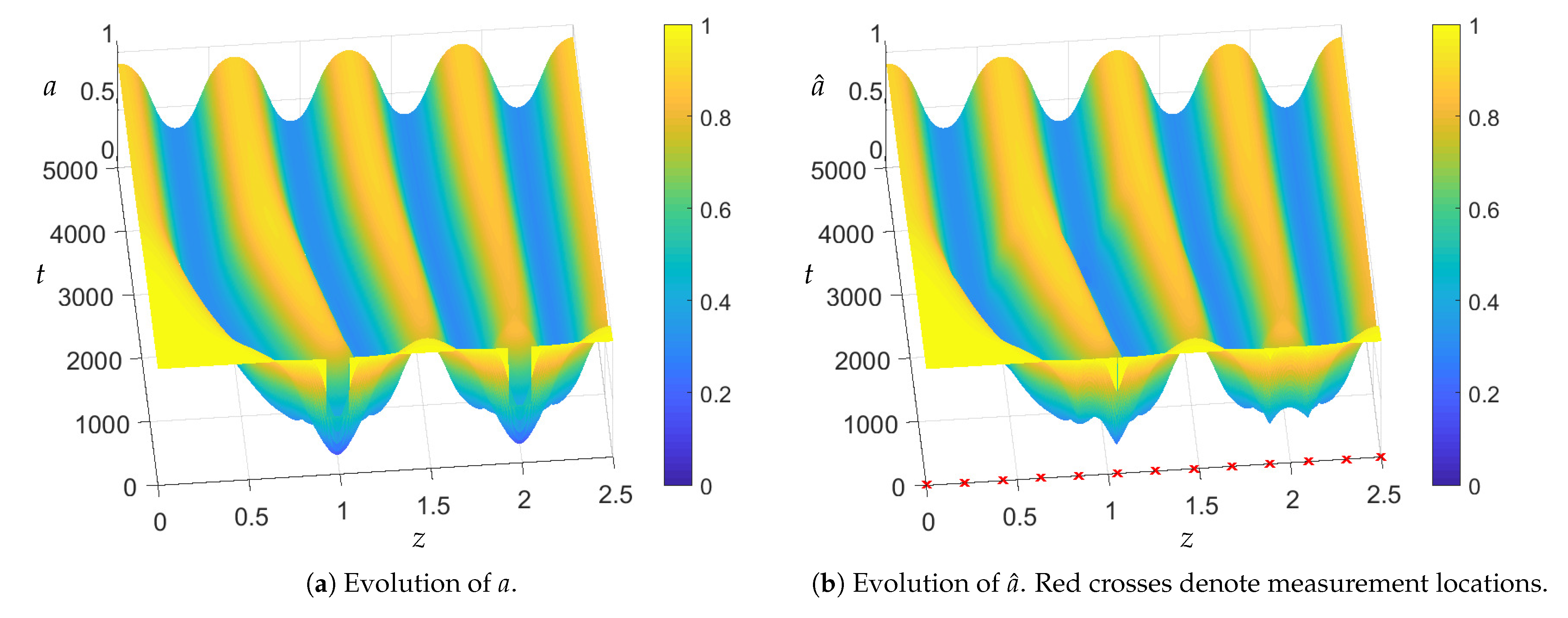
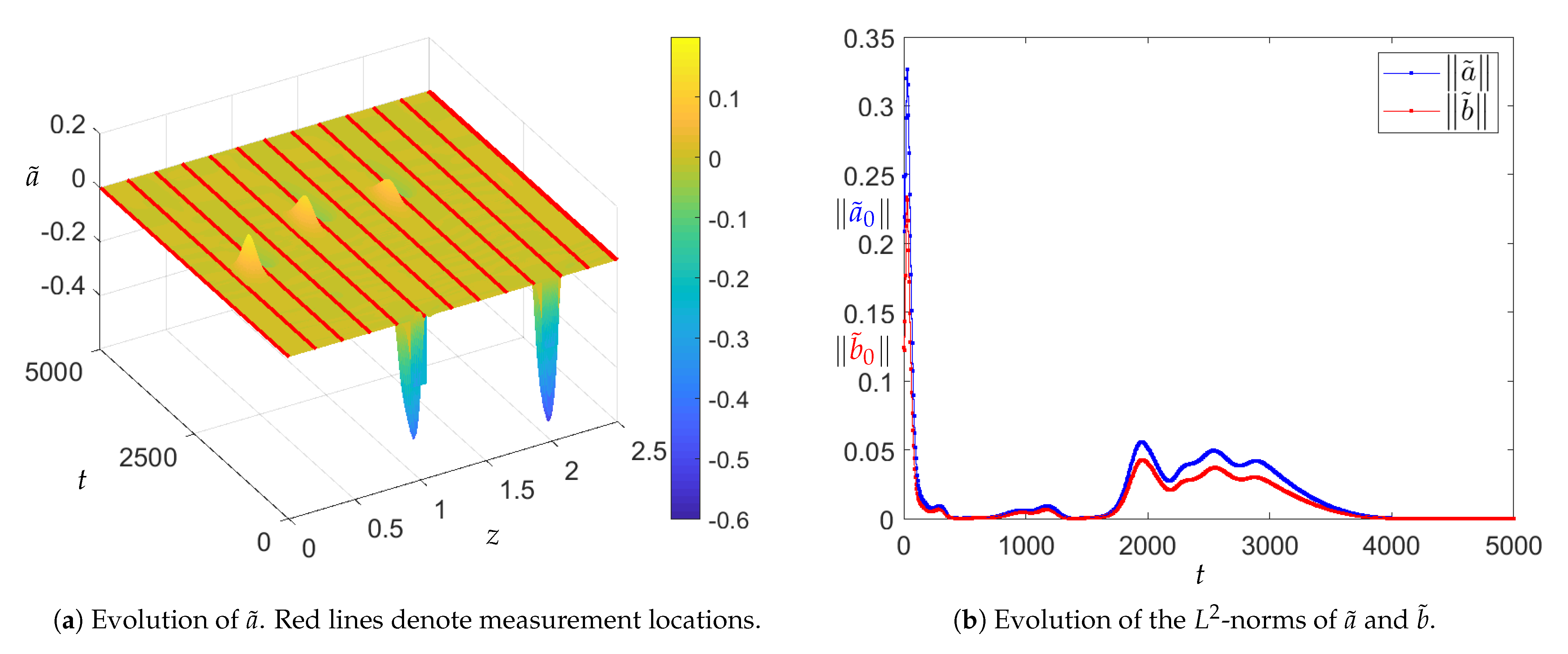
Model (1) is considered on the domain $\Omega =(0,2.5)$ with parameters $D_a=2\times {10}^{-4}$, $D_b=1\times {10}^{-4},\alpha =0.02951,\beta =0.058$ and the initial conditions $(a_0,b_0)=(1,0)$ which are perturbed to $(a_0\left(z\right),b_0\left(z\right))=(0.5,0.25)$ at locations $z\in (0.925,1.05)$ and $z\in (1.925,2.05)$ (see Figure 1a). The corresponding stationary pattern is depicted in Figure 1b. Thirteen measurement points are distributed uniformly over $\Omega$. The initial values for the observer are selected at the steady state $({\widehat{a}}_0,{\widehat{b}}_0)=(1,0)$. The evolution of the system and the observer states are depicted in Figure 2. The corresponding observation errors are given in Figure 3 showing the convergence of their norms to zero as $t\to \infty$. All simulations in Example 1 (and Example 2) are performed in Matlab using pdepe-function and approximate solutions are plotted on ${10}^3\times {10}^3$ space-time discretization mesh.

3.2. Example 2 (Non-Stationary Pattern)

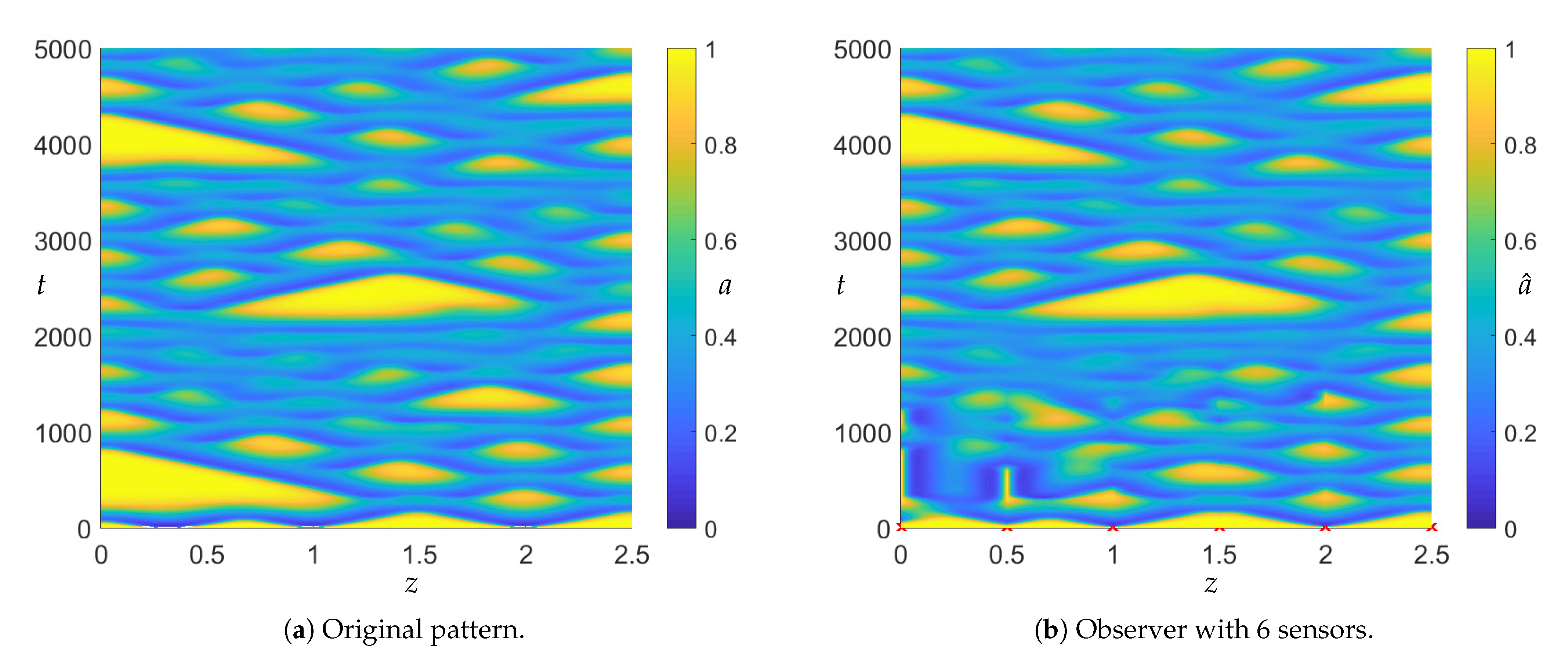
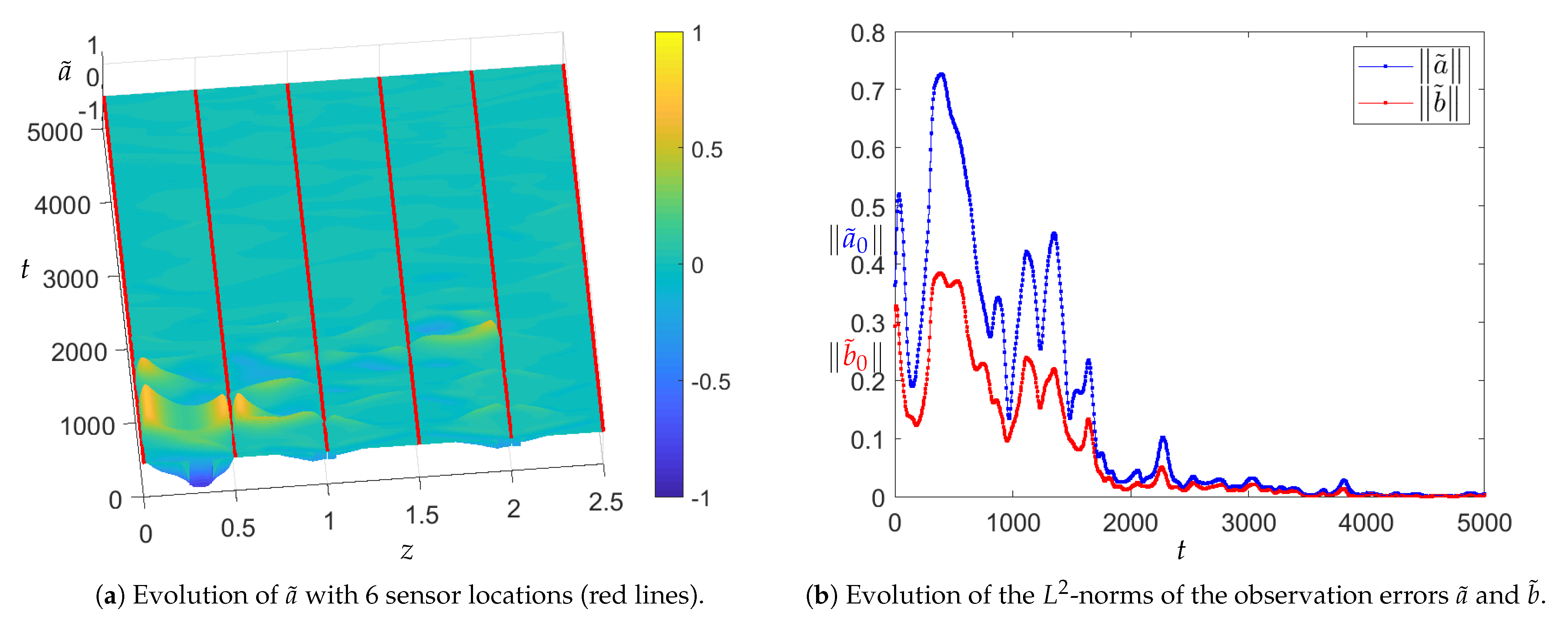
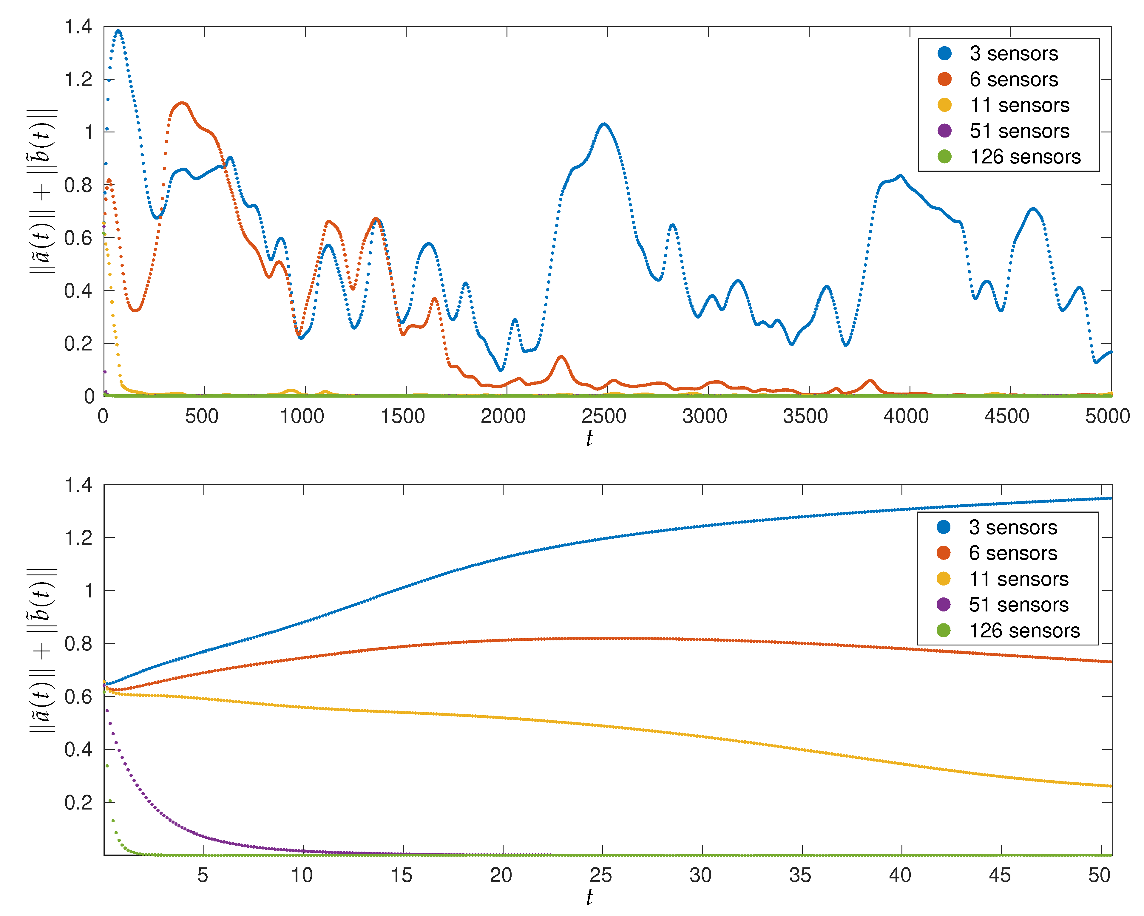
Model (1) is considered in the domain $\Omega =(0,2.5)$ with parameters $D_a=2\times {10}^{-4},D_b=1\times {10}^{-4},\alpha =0.02,\beta =0.047$ and the initial conditions $(a_0,b_0)=(1,0)$ which are perturbed to $(a_0\left(z\right),b_0\left(z\right))=(0.5,0.25)$ at locations $z\in (0.925,1.05)$ and $z\in (1.925,2.05)$ and to $(a_0\left(z\right),b_0\left(z\right))=(0.25,0.75)$ at locations $z\in (0.25,0.375)$. A comparison of the original behavior and the observer with six uniformly distributed sensors is given in Figure 4 and the corresponding observation errors are provided in Figure 5. The norms of these errors converge to zero as $t\to \infty$. Additionally, the observation errors for the observers with 3, 6, 11, 51, and 126 equidistant measurement locations are depicted in Figure 6. These numerical simulations demonstrate that the smaller gaps $d_i$ between sensors lead to smaller observation errors and their faster convergence to 0. This convergence is exponential provided a sufficiently large number of sensors is used, i.e., the distances $d_i$ between sensors satisfy (16). The initial conditions for all observers are selected at the steady state $({\widehat{a}}_0,{\widehat{b}}_0)=(1,0)$.

For the system parameters $D_a,D_b,\alpha ,\beta$, and initial conditions used in Examples 1 and 2, the uniform bounds of the concentrations can be taken as ${\overline{h}}_a={\overline{h}}_b=1$. Then, (16) suggests that 125 sensors are required to guarantee the convergence of the observer’s state to the real states of both systems from Examples 1 and 2. The simulations, however, show that 13 and 6 sensors are sufficient for Example 1 and Example 2, respectively. There are two reasons for this conservatism: (i) Lipschitz-type estimates of the reaction nonlinearities and rough estimates of their gradients; (ii) Theoretical results guarantee the convergence of the error for any initial conditions, while the simulations use particular ones.

Taking this into account, the theoretical result of the current paper provides a fundamental statement on the possibility of pattern reconstruction by choosing a sufficiently large number of measurement points. For the simulations and real experiments this number can be considered as a tuning parameter. Interestingly, if the number of sensors is less than the value required to satisfy (16), the non-stationary patterns and spatiotemporal chaotic behavior are more likely to be properly tracked with the observer (5) compared to the asymptotically stable stationary patterns. The reason for this is that the perturbation terms $\Delta {\phi }_i$ in (8) oscillate in a relatively wide range of values for the case of non-stationary behavior whilst these terms can be permanently large in particular spatial intervals ${\mathcal{I}}_i$ when the state profile is close to the stationary pattern. In these intervals, the observer state may diverge from the real state if the corresponding $d_i$, $i=1,\dots ,m$ are larger than the required theoretical value defined in (16).

4. Conclusions and Outlook

The paper proposes a constructive state estimation technique for the one-dimensional Gray–Scott model utilizing the state measurements at a finite number of spatial locations. Sufficient conditions are derived which ensure the exponential convergence of the estimated state to the original one. The proposed state reconstruction technique can be utilized for the feedback control schemes which require the knowledge of the complete state of the system. Complete state feedback of reaction-diffusion systems are often used for the control of semiconductor nanostructures [38] and particular examples of the control of patterns in the Gray–Scott model via delayed state feedback can be found in [21]. In addition, inequalities (16a) and (16b) can be reformulated as sufficient conditions for the synchronization of the master-slave configuration of two identical 1D Gray–Scott models coupled via a finite number of spatial locations.

It is of interest to obtain more precise estimates of the invariant subspaces for the concentrations a, b, and $a+b$ depending on the system parameters, initial conditions, and spatial interval. Numerical simulations of [3,5] suggest that neither a nor b are $\mathcal{O}\left(1\right)$ throughout the whole pattern. For instance, during a peak in b, it has been observed that b is ‘large’, while a becomes ‘small’. This additional information might lead to more precise estimates of the constants $L^a,L^b$ used in the proof of Theorem 1. Also, it is of interest to study possible improvements of the observer’s performance by adding an output injection term (i.e., the difference between the measured and estimated output weighted with some observer gain) directly into the observer PDEs and by optimizing the non-uniform spacing between measurement locations. Another challenging direction is the observer design with a finite number of measurement locations for the Gray–Scott model defined in 2D and higher-dimensional spatial domains.

The observer design approach proposed in this paper assumes the knowledge of the model and all its parameters. This assumption may not always be compatible with real applications and experimental setups. Therefore, a fusion of the proposed state estimation technique with the simultaneous parameter identification could be of interest for future research.

References

- Gray, P.; Scott, S. Autocatalytic reactions in the isothermal, continuous stirred tank reactor: Oscillations and instabilities in the system A+ 2B→3B; B→C. Chem. Eng. Sci. 1984, 39, 1087–1097. [Google Scholar] [CrossRef]
- McGough, J.S.; Riley, K. Pattern formation in the Gray–Scott model. Nonlinear Anal. Real World Appl. 2004, 5, 105–121. [Google Scholar] [CrossRef]
- Doelman, A.; Kaper, T.J.; Zegeling, P.A. Pattern formation in the one-dimensional Gray-Scott model. Nonlinearity 1997, 10, 523. [Google Scholar] [CrossRef]
- Nishiura, Y.; Ueyama, D. Spatio-temporal chaos for the Gray–Scott model. Phys. D 2001, 150, 137–162. [Google Scholar] [CrossRef]
- Reynolds, W.N.; Pearson, J.E.; Ponce-Dawson, S. Dynamics of self-replicating patterns in reaction diffusion systems. Phys. Rev. Lett. 1994, 72, 2797. [Google Scholar] [CrossRef]
- Kolokolnikov, T.; Wei, J. On ring-like solutions for the Gray–Scott model: Existence, instability and self-replicating rings. Eur. J. Appl. Math. 2005, 16, 201–237. [Google Scholar] [CrossRef] [Green Version]
- Delgado, J.; Hernández-Martínez, L.I.; Pérez-López, J. Global bifurcation map of the homogeneous states in the Gray–Scott model. Int. J. Bifurc. Chaos 2017, 27, 1730024. [Google Scholar] [CrossRef] [Green Version]
- You, Y. Global attractor of the Gray-Scott equations. Commun. Pure Appl. Anal. 2008, 7, 947. [Google Scholar] [CrossRef]
- Morgan, D.S.; Kaper, T.J. Axisymmetric ring solutions of the 2D Gray–Scott model and their destabilization into spots. Phys. D 2004, 192, 33–62. [Google Scholar] [CrossRef] [Green Version]
- Muratov, C.; Osipov, V.V. Static spike autosolitons in the Gray-Scott model. J. Phys. A 2000, 33, 8893. [Google Scholar] [CrossRef]
- Wei, J.; Winter, M. Asymmetric spotty patterns for the Gray–Scott model in ℝ2. Stud. Appl. Math. 2003, 110, 63–102. [Google Scholar] [CrossRef]
- Ouyang, Q.; Swinney, H.L. Transition from a uniform state to hexagonal and striped Turing patterns. Nature 1991, 352, 610–612. [Google Scholar] [CrossRef]
- Pearson, J.E. Complex patterns in a simple system. Science 1993, 261, 189–192. [Google Scholar] [CrossRef] [PubMed] [Green Version]
- Wang, W.; Lin, Y.; Yang, F.; Zhang, L.; Tan, Y. Numerical study of pattern formation in an extended Gray–Scott model. Commun. Nonlinear Sci. Numer. Simul. 2011, 16, 2016–2026. [Google Scholar] [CrossRef]
- Vigelius, M.; Meyer, B. Stochastic simulations of pattern formation in excitable media. PLoS ONE 2012, 7, e42508. [Google Scholar] [CrossRef] [Green Version]
- Lee, K.J.; McCormick, W.; Ouyang, Q.; Swinney, H.L. Pattern formation by interacting chemical fronts. Science 1993, 261, 192–194. [Google Scholar] [CrossRef] [Green Version]
- Lee, K.J.; McCormick, W.D.; Pearson, J.E.; Swinney, H.L. Experimental observation of self-replicating spots in a reaction–diffusion system. Nature 1994, 369, 215–218. [Google Scholar] [CrossRef]
- Hankins, S.N.; Fertig, R.S., III. Methodology for optimizing composite design via biological pattern generation mechanisms. Mater. Des. 2021, 197, 109208. [Google Scholar] [CrossRef]
- Vigneresse, J.L.; Truche, L. Modeling ore generation in a magmatic context. Ore Geol. Rev. 2020, 116, 103223. [Google Scholar] [CrossRef]
- Sherratt, J.A.; Mackenzie, J.J. How does tidal flow affect pattern formation in mussel beds? J. Theor. Biol. 2016, 406, 83–92. [Google Scholar] [CrossRef]
- Kyrychko, Y.; Blyuss, K.; Hogan, S.; Schöll, E. Control of spatiotemporal patterns in the Gray–Scott model. Chaos 2009, 19, 043126. [Google Scholar] [CrossRef] [Green Version]
- Xie, W.X.; Cao, S.P.; Cai, L.; Zhang, X.X. Study on Turing Patterns of Gray–Scott Model via Amplitude Equation. Int. J. Bifurc. Chaos 2020, 30, 2050121. [Google Scholar] [CrossRef]
- Zhang, K.; Liu, X.; Xie, W.C. Impulsive Control and Synchronization of Spatiotemporal Chaos in the Gray–Scott Model. In Interdisciplinary Topics in Applied Mathematics, Modeling and Computational Science; Springer: New York, NY, USA, 2015; pp. 549–555. [Google Scholar]
- Zhang, K. Impulsive Control of Dynamical Networks. Ph.D. Thesis, University of Waterloo, Waterloo, ON, Canada, 2017. [Google Scholar]
- Torres, L.; Besancon, G.; Verde, C.; Georges, D. Parameter identification and synchronization of spatio-temporal chaotic systems with a nonlinear observer. IFAC Proc. Vol. 2012, 45, 267–272. [Google Scholar] [CrossRef]
- Torres, L.; Besançon, G.; Verde, C.; Guerrero-Castellanos, J.F. Generalized synchronization of a class of spatiotemporal chaotic systems using nonlinear observers. Int. J. Bifurc. Chaos 2015, 25, 1550149. [Google Scholar] [CrossRef]
- Torres, L.; Besançon, G.; Georges, D.; Verde, C. Exponential nonlinear observer for parametric identification and synchronization of chaotic systems. Math. Comput. Simul. 2012, 82, 836–846. [Google Scholar] [CrossRef]
- Schaum, A.; Alvarez, J.; Meurer, T.; Moreno, J. State-estimation for a class of tubular reactors using a pointwise innovation scheme. J. Process Control 2017, 60, 104–114. [Google Scholar] [CrossRef]
- Schaum, A.; Moreno, J.A.; Alvarez, J.; Meurer, T. A simple observer scheme for a class of 1-D semi-linear parabolic distributed parameter systems. In Proceedings of the 2015 European Control Conference (ECC), Linz, Austria, 15–17 July 2015; pp. 49–54. [Google Scholar]
- Schaum, A.; Alvarez, J.; Meurer, T.; Moreno, J. Pointwise innovation–based state observation of exothermic tubular reactors. IFAC-PapersOnLine 2016, 49, 955–960. [Google Scholar] [CrossRef]
- Schaum, A. An unknown input observer for a class of diffusion-convection-reaction systems. at-Automatisierungstechnik 2018, 66, 548–557. [Google Scholar] [CrossRef]
- Pierre, M. Global existence in reaction-diffusion systems with control of mass: A survey. Milan J. Math. 2010, 78, 417–455. [Google Scholar] [CrossRef]
- Hollis, S.L.; Martin, R.H., Jr.; Pierre, M. Global existence and boundedness in reaction-diffusion systems. SIAM J. Math. Anal. 1987, 18, 744–761. [Google Scholar] [CrossRef]
- Mironchenko, A.; Karafyllis, I.; Krstic, M. Monotonicity methods for input-to-state stability of nonlinear parabolic PDEs with boundary disturbances. SIAM J. Control Optim. 2019, 57, 510–532. [Google Scholar] [CrossRef]
- Delattre, C.; Dochain, D.; Winkin, J. Sturm-Liouville systems are Riesz-spectral systems. Int. J. Appl. Math. Comput. Sci. 2003, 13, 481–484. [Google Scholar]
- Curtain, R.F.; Zwart, H. An Introduction to Infinite-Dimensional Linear Systems Theory; Springer: New York, NY, USA, 1995. [Google Scholar]
- Pazy, A. Semigroups of Linear Operators and Applications to Partial Differential Equations; Springer: New York, NY, USA, 1992. [Google Scholar]
- Franceschini, G.; Bose, S.; Schöll, E. Control of chaotic spatiotemporal spiking by time-delay autosynchronization. Phys. Rev. E 1999, 60, 5426. [Google Scholar] [CrossRef]
Figure 1.
Typical patterns generated by the Equation (1) in the interval (0, 2.5) with diffusion coefficients Da = 2 × 10⁻⁴ and Db = 10−4. Both patterns (b,c) emerge from the same initial conditions (a) but for different sets of parameters α, β.
Figure 2.
A comparison of the evolution of the system and the observer states for Example 1.
Figure 3.
Observation errors for Example 1.
Figure 4.
A comparison of the original evolution of a and for the observers with 6 measurement locations for Example 2.
Figure 5.
Observation errors for the observer with 6 sensors for Example 2.
Figure 6.
Evolution of (i.e., the sum of -norms of the observation errors) for Example 2 depending on the number of equidistantly located sensors for (top figure) and (bottom figure). The observer with 3 sensors does not converge to the original system, whereas all other observers converge to the original system with the convergence rate increasing with the number of sensors.
Publisher’s Note: MDPI stays neutral with regard to jurisdictional claims in published maps and institutional affiliations. |
© 2021 by the authors. Licensee MDPI, Basel, Switzerland. This article is an open access article distributed under the terms and conditions of the Creative Commons Attribution (CC BY) license (https://creativecommons.org/licenses/by/4.0/).
Share and Cite
MDPI and ACS Style
Feketa, P.; Schaum, A.; Meurer, T. Distributed Parameter State Estimation for the Gray–Scott Reaction-Diffusion Model. Systems 2021, 9, 71. https://0-doi-org.brum.beds.ac.uk/10.3390/systems9040071
AMA Style
Feketa P, Schaum A, Meurer T. Distributed Parameter State Estimation for the Gray–Scott Reaction-Diffusion Model. Systems. 2021; 9(4):71. https://0-doi-org.brum.beds.ac.uk/10.3390/systems9040071
Chicago/Turabian StyleFeketa, Petro, Alexander Schaum, and Thomas Meurer. 2021. "Distributed Parameter State Estimation for the Gray–Scott Reaction-Diffusion Model" Systems 9, no. 4: 71. https://0-doi-org.brum.beds.ac.uk/10.3390/systems9040071
Note that from the first issue of 2016, this journal uses article numbers instead of page numbers. See further details here.