Facial Expression Emotion Detection for Real-Time Embedded Systems †


1
Department of Electronic and Computer Engineering, Brunel University London, Uxbridge UB8 3PH, UK
2
Department of Electronics and Multimedia Telecommunications, Technical University of Kosice, Letna 9, 04001 Kosice, Slovakia
*
Author to whom correspondence should be addressed.
†
This paper is an extended version of our paper in Proceedings of Innovative Computing Technology (INTECH 2017), Luton, UK, 16–18 August 2017; with permission from IEEE.
Technologies 2018, 6(1), 17; https://0-doi-org.brum.beds.ac.uk/10.3390/technologies6010017
Submission received: 15 December 2017
/
Revised: 13 January 2018
/
Accepted: 22 January 2018
/
Published: 26 January 2018
(This article belongs to the Special Issue Selected Papers from the Seventh International Conference on Innovative Computing Technology (INTECH 2017))
Abstract
:Recently, real-time facial expression recognition has attracted more and more research. In this study, an automatic facial expression real-time system was built and tested. Firstly, the system and model were designed and tested on a MATLAB environment followed by a MATLAB Simulink environment that is capable of recognizing continuous facial expressions in real-time with a rate of 1 frame per second and that is implemented on a desktop PC. They have been evaluated in a public dataset, and the experimental results were promising. The dataset and labels used in this study were made from videos, which were recorded twice from five participants while watching a video. Secondly, in order to implement in real-time at a faster frame rate, the facial expression recognition system was built on the field-programmable gate array (FPGA). The camera sensor used in this work was a Digilent VmodCAM — stereo camera module. The model was built on the Atlys™ Spartan-6 FPGA development board. It can continuously perform emotional state recognition in real-time at a frame rate of 30. A graphical user interface was designed to display the participant’s video in real-time and two-dimensional predict labels of the emotion at the same time.
1. Introduction
Since the last decade, studies on human facial emotion recognition have revealed that computing models based on regression modeling can produce applicable performance [1]. Emotion detection and recognition were introduced by researches with human observers [2,3]. Automatic recognition and the study of the facial emotional status represent substantial suggestions for the way in which a person performs, and these are very helpful for detecting, inspection and keeping safe vulnerable persons such as patients who experience mental issues, persons who endure significant mental pressure, and children with less ability to control themselves. With emotion recognition ability, machines such as computers, robots, toys and game consoles will have the capability to perform in such a way as to influence the user in adaptive ways relevant for the client’s mental condition. This is the key knowledge in recently proposed new ideas such as emotional computers, emotion-sensing smart phones and emotional robots [4]. Over the last decade, most studies have focused on emotional symptoms in facial expressions. In recent years, scientists have studied effective transition through body language. The recognition of entire body gestures is expressively more difficult, as the shape of the human body has more points of freedom than the face, and its overall outline differs muscularly through representative motion. The research presented in this paper is an extension of our previous conference article [5].
In the 19th century, one of the significant works on facial expression analysis that has a straight association to the current state-of-the-art in automatic facial expression recognition was the effort made by Charles Darwin, who, in 1872, wrote a dissertation that recognized the general values of expression and the incomes of expressions in both humans and animals [6]. Darwin grouped several kinds of terms into similar groups. The classification is as follows:
- low spirits, anxiety, grief, dejection and despair;
- joy, high spirits, love, tender feelings and devotion;
- reflection, meditation, ill-temper and sulkiness;
- hatred and anger;
- disdain, contempt, disgust, guilt and pride;
- surprise, astonishment, fear and horror;
- self-attention, shame, shyness and modesty.
Darwin also classified the facial distortions that happen for each of the above-stated classes of expressions. For example, “the constriction of the muscles around the eyes when in sorrow”, “the stiff closure of the mouth when in contemplation”, and so forth [6]. Another considerable landmark in the researching of facial expressions and human emotions has been the work of Paul Ekman and his colleagues since the 1970s. Their work has had a massive effect on state-of-the-art automatic facial expression recognizer development.
The earliest study of facial expression automatic recognition was realized in 1978 by Suwa et al. [7], who generated a model for studying facial expressions from a sequence of pictures by employing 20 tracking arguments. Research was conducted until the end of the 1980s and early 1990s, when the economy’s computing power on-the-go became available. This helped to grow face-detection and face-tracking algorithms in the early 1990s. At the same time, human–computer interaction (HCI) and affective computing (AC) research began [4].
Paul Ekman and his colleagues classified the basic emotions, and their work has had a significant impact on the current emotion analysis development [8]. Emotional state analysis is most likely a psychology field. However, as a result of more and more computing methods being successfully used in this area, it has been merged into a computing topic with the new name of AC [9]. Signal and image processing and pattern recognition methods deliver a fundamental role for efficient computing. Firstly, the emotional state of a person can be detected from their facial expression, speech and body gestures by imaging systems. Secondly, the features can be extracted from these recordings on the basis of signal and image processing methods. Finally, advanced pattern recognition methods are applied to recognize the emotional states.
As far as is known, this is the first time that automatic emotional state detection has been successfully implemented on an embedded device (the field-programmable gate array—FPGA). The proposed system is 20 times faster than the Graphics Processing Unit (GPU) implementation [10] and can analyze 30 frames per second in real-time. In this paper, the technique’s implementation and the evaluation of both results are presented. The system is able to display the real-time and automatic emotional state detection model on the connected monitor.
2. Related Work
In contemporary psychology, affect is known as the experience of sensation or emotion as different from thought, belief, or action. Therefore, emotion is the sense that a person feels, while affect is in terms of state. Scherer defines emotion as the outcome of reaction synchronization whose output corresponds to an event that is “relevant to the major concerns of the organism” [11]. Emotion is different from mood in that the former has a strong and clear attention while the latter is unclear, can appear without reason, and can lack severity. Psychologists perceive moods as “diffuse affect states, characterized by a relative enduring predominance of certain types of subjective feelings that affect the experience and behaviour of a person” [11]. Moods may carry for hours or days; as a result of people’s characters and affect natures, some people practice some moods more often than others [11]. Consequently it is more problematic to measure situations of mood. On the other hand, emotion is a quantifiable element because of its separate nature.
Primary attempts to measure and classify feeling through the perception of facial expressions has revealed that feelings are not the result of the retraction of only one muscle; nonetheless particular sets of muscles cause facial expressions to reveal these feelings. In 1872, Darwin postulated on his original work that facial expressions in people were the result of improvements and that: “The study of expression is difficult, owing to the movements (of facial muscles) being often extremely slight, and of a fleeting nature” [12]. Notwithstanding this test, early efforts to measure emotions on the basis of facial expressions in adults and infants were realized. Initial research on undesirable emotional states has proved that particular features of the eyelids and eyebrows, which Darwin called “the grief-muscles”, agree in that “oblique position in persons suffering from deep dejection or anxiety” [12]. However, scientists during the 19th century were faced with challenges to separate emotional states, recognizing distinctions between perceptions and intentions. “A difference may be clearly perceived, and yet it may be impossible, at least I have found it so, to state in what the difference consists” [12]. Darwin considered general facial muscles, which were involved in each of the emotions’ state (Table 1).
Significant improvements have been completed in the measurement of individual elements of emotion. Ekman‘s Facial Action Coding System (FACS) [13] relates the observation of particular muscle contractions of the face with emotions. Scherer et al. measured emotions using an assessment of defined components [14]; Davidson et al. published comprehensive studies on the relation between brain physiology and emotional expressions [15]; Stemmler‘s studies determined and revealed physiological reaction outlines [16]; Harrigan et al. carried out an appraisal and measured adequate behaviour [17]; and Fontaine et al. presented that in order to demonstrate the six components of feelings, at least four dimensions are needed [14]. These studies demonstrate that although emotions are various and multifaceted, and also often problematic to classify, they present themselves via designs that “in principle can be operationalized and measured empirically” [11]. The difficulty of classifying these patterns is what drives research in emotional computing. In the last 20 years, the majority of the study in this area has been into enabling processors and computers to declare and identify affect [9]. Progress made in emotional computing has not only assisted its own research field, but also benefits practical domains such as computer interaction. Emotional computing research develops computer interaction by generating computers to improve services the user desires. Meanwhile, it has also allowed humans to perceive computers as something more than merely data machines. Upgrading computer interaction over emotional computing studies has various benefits, from diminishing human users’ frustration to assisting machines’ familiarization with their human users by allowing the communication of user feeling [9]. Emotional computing enables machines to become allied operative systems as socially sagacious factors [18].
This helped in the early 1990s [7] to grow face-detection [19] and -tracking results in HCI and AC [9] evolution. The emotions of the user could be detected using advanced pattern recognition algorithms from extracted images (facial expression, gestures, etc.) or audio (speech) features. Recently, Cambridge University introduced the emotional computer [20] and the MIT (Massachusetts Institute of Technology) Mood Meter [21] From 2011, these have participated in several international emotion recognition challenges, such as AVEC (Audio/Visual Emotion Challenge) or MediaEval (Benchmarking Initiative for Multimedia Evaluation) [22,23].
In 2013, Cheng, J., et al. [10] proposed the GP-GPU (General Purpose - Graphics Processing Unit) acceleration service for continuous face- and emotion-detection systems. Promising results were achieved for the real-world scenario of continuous movie scene monitoring. The system was initially tested in MATLAB. It was proven that the GPU acceleration could speed up the processing 80-fold compared to the CPU (Central Processing Unit). This system can provide the detected emotional state every 1.5 s.
In 2015, the Microsoft Oxford API (Application Programming Interface) cloud service provided the recognition of emotions on the basis of facial expressions [24]. This API provides the confidence across a set of emotions for each face in the image, as well as bounding box for the face. The emotions detected are anger, contempt, disgust, fear, happiness, neutrality, sadness, and surprise. These emotions are understood to be cross-culturally and universally communicated with facial expressions. Recognition is experimental and is not always accurate [24]. Recently, fuzzy support vector machines (SVMs) and feed-forward neural networks together with a stationary wavelet entropy approach were investigated, producing results of around 96% accuracy on stationary images [25,26].
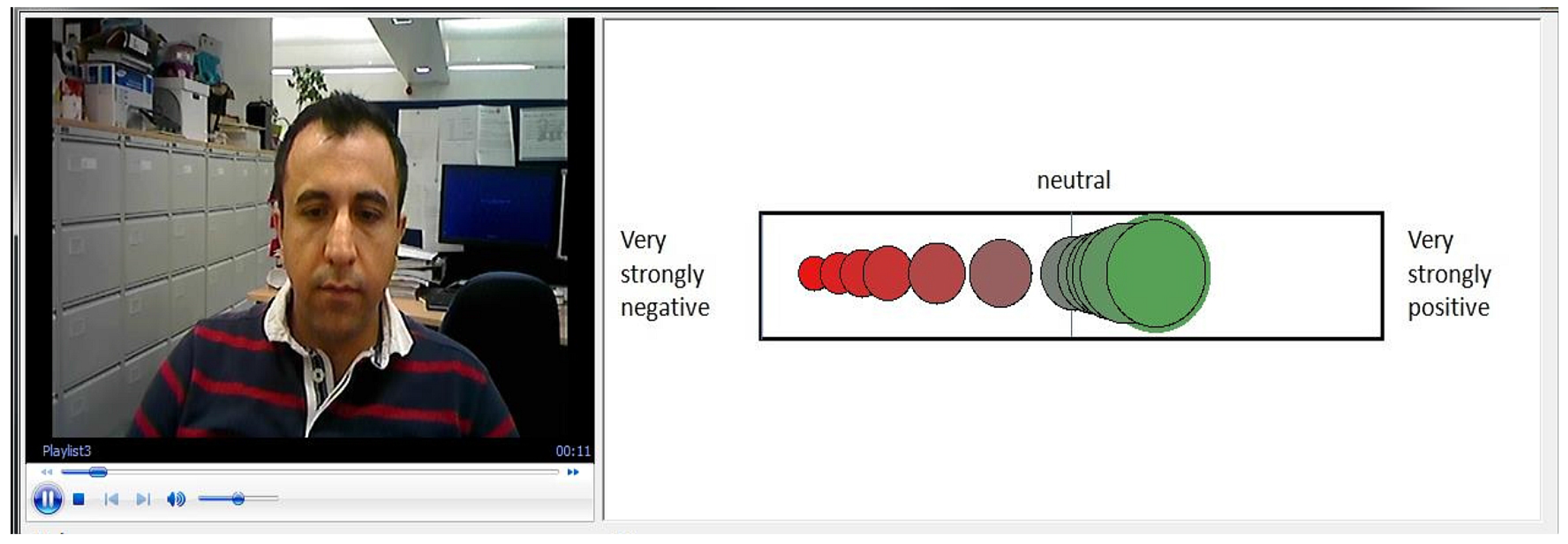
Several tools have been developed to record perceived emotions as specified by the four emotional dimensions. FeelTrace is a tool created on a two-dimensional space (activation and evaluation), which allows an observer to “track the emotional content of a stimulus as they perceive it over time” [27]. This tool offers the two emotional dimensions as a rounded area on a computer screen. Human users of FeelTrace observe a stimulus (e.g., watching a program on TV, listening to an affective melody or the display of strong emotions) and move a mouse cursor to a place within the circle of the emotional area to label how they realize the incentive as time continues. The measurement of time is demonstrated indirectly by tracing the position at which the mouse is in the circle with time measured in milliseconds. Arrangements using the FeelTrace classification were used to create the labels in the testing described in this paper. In Figure 1 is an example of a FeelTrace exhibition while following a session. The color-coding arrangement allows users to label the extensity of their emotion. Pure red represents the most negative assessment in the activation (very active) dimension; pure green represents when the user is feeling the most positive evaluation in the activation dimension (very passive). FeelTrace allows its users to produce annotations of how they observe specific stimuli at specific points in time. The system has been shown to be able to perceive the changing of emotions over time.
The proposed local binary pattern (LBP) algorithm uses the alteration of an image into an arrangement of micropatterns. The performance with face images is described in [28]. The typical LBP algorithm executes calculations inside a local region (“neighbourhood block”) of all the pixels in a grayscale image (which is initially delivered into MATLAB as numerical values instead of the intensity levels of RGB (Red Green Blue), which are then changed to grayscale intensity numerical values). The working out algorithm results in numerical values, which are demonstrated as alternation counts in a histogram. The alternation counts from the histogram are the components of a row vector. The row vectors of each block are horizontally concatenated together to form a single feature vector, which is a descriptor for the entire image. There are numerous differences of LBP algorithms in the present literature. The method described in this paper uses features obtained by uniform LBPs [29]. Uniform LBP is similar to the basic LBP, except that the dimensionality of the feature vectors is cut in order to keep computational time minimal and to lower the memory usage.
On the other hand, the k-Nearest Neighbor algorithm (k-NN) is utilized for regression modeling [30]. This algorithm is based on learning, where the operation is only approximated nearby the training dataset and all calculations are delayed until regression. The k-NN regression is typically based on the distance between a query point (test sample) and the specified samples (training dataset). There are many methods available to measure this distance, for example, Euclidean squared, city-block, and Chebyshev methods. One of the most common choices to obtain this distance is the Euclidean method: Let be an input sample with P features ( ), n be the total number of input samples (), and p be the total number of features (). Therefore, the Euclidean distance between the samples and () can be defined by Equation (1):
Cross-validation is a typical confirmation method for measuring the outcomes of a numerical investigation, which distributes to an independent dataset. It is usually implemented whenever the aim is prediction, and the purpose of using cross-validation is to estimate how precisely the predictive system will implement and perform in practice and in real-time. In predictive models, a system is typically given a specified dataset called a training dataset and a testing dataset against which the system is verified [31,32]. The aim of this method is to express a dataset to check the system in the training dataset in order to reduce problems. Additionally, one of the main reasons that the cross-validation method is used in this study is that it is a valuable estimator of the system performance; therefore, the fault on the test dataset correctly characterizes the valuation of the system performance. This is due to there being sufficient data accessible and/or that there is a well re-partition and good separation of the data into training and test sets. Thus cross-validation is a reasonable method to accurately estimate the prediction of a system.
3. Affective Dimension Recognition
In effective dimensional space, more details on how the emotional states other than the six basic emotion categories (i.e., happy, sad, disgust, anger, surprise and fear) are represented. The three-dimensional (3D) model contains arousal, dominance and valence. Therefore, the automatic emotional state detection system needs to comprehensively model the variations in visuals and convert these to the arousal, dominance and valence scale from the captured video. From the machine learning point of view, this is not a classification problem but a regression problem, because the predicted values are real numbers on each individual frame in the image sequence.
The inputs into the merger system are the videos recorded from five volunteers, which were used to build the system training part, each recorded twice while a 210 s video was watched. Therefore there are 10 videos recorded at 25 frames per second (52,500 frames in total). For the MATLAB system, 5-fold cross-validation and then 2-fold cross-validation were implemented. GTrace was employed in order to obtain and build the training datasets. LBP features were extracted from the videos. We note that LBP is the most common feature extraction that has been used in numerous emotional state recognition systems. A k-NN algorithm was used for the regression because of its simplicity and lesser complexity to implement on FPGA compared to other algorithms. At the training phase, features were extracted from image sequences from the 10 videos. At the testing step, features of the new image from a camera connected to FPGA were calculated and sent to the k-NN for regression with dimensional emotion labels (e.g., real values for activation and valence) as the output. As the training set was complete, the entire system was expected to produce incessant dimensional labels.
3.1. System Overview
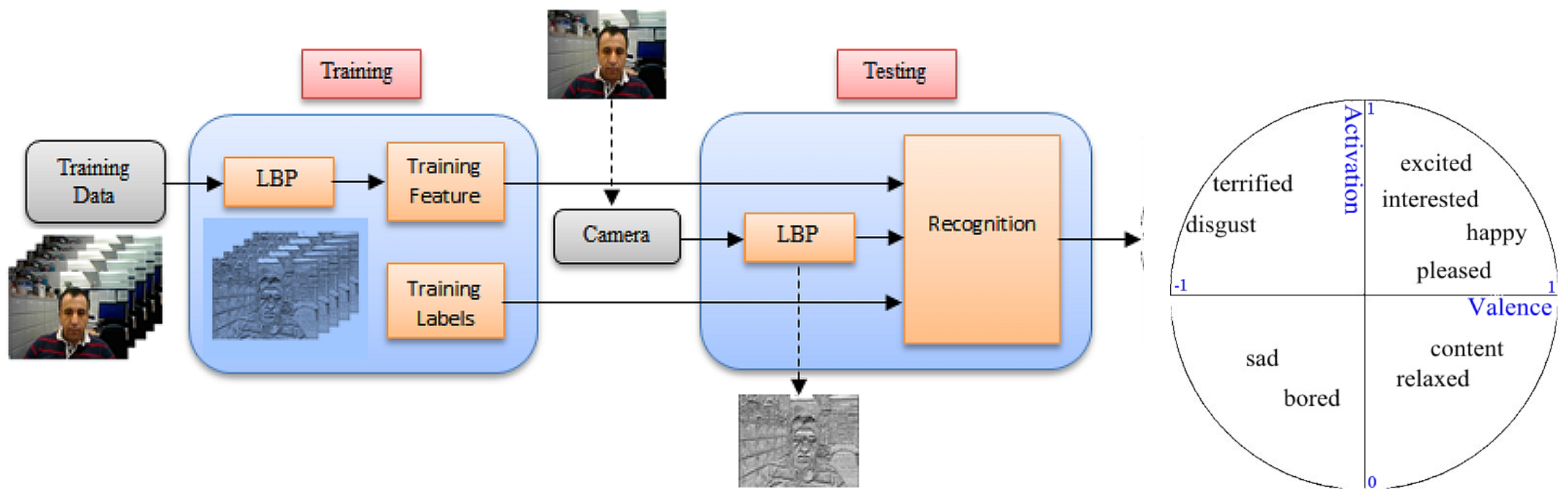
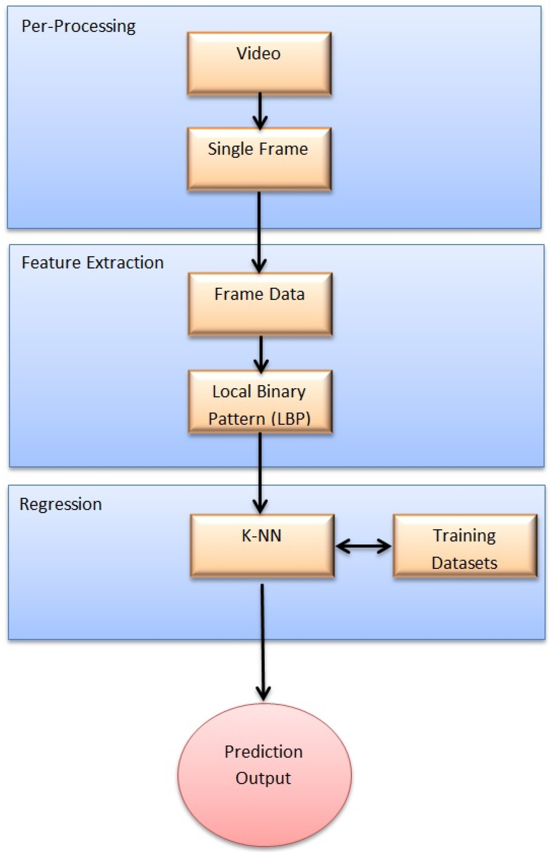
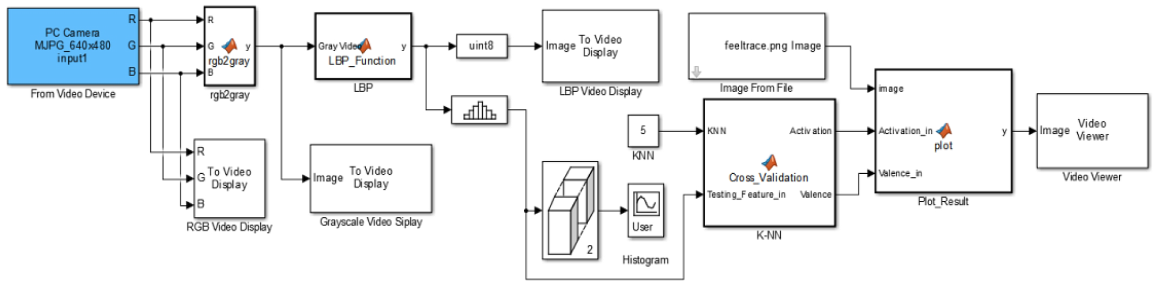
In Figure 2, the framework of the automatic emotional state detection system is depicted. The inputs are the video frames captured from the camera. FeelTrace [27] was used to capture the videos and extract the training datasets. LBP features were extracted from the captured videos. The k-NN algorithm was used for regression. For training, the LBP features were extracted from 10 video image sequences. Video captures from the FPGA connected camera were processed, and the LBP features were used for the k-NN regression with dimensional emotion labels.
3.2. Image Feature Extraction
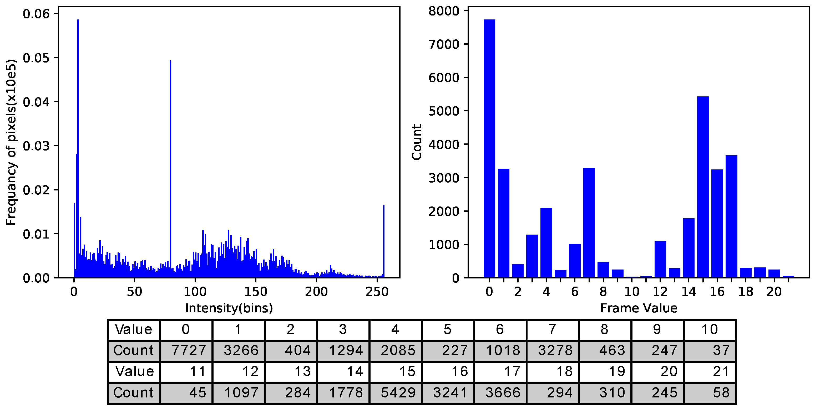
The LBP algorithm converts local sub-blocks of the grayscale converted image to an alternation counts histogram. The histogram values of each block were horizontally concatenated together to form a single feature vector, which is the descriptor for the entire image. There are numerous differences in LBP algorithms in the present literature [33]. The method described in this paper uses features obtained by uniform LBP [29]. Uniform LBP uses dimensionally reduced feature vectors in order to save computational time and memory. In this work, the standard LBP algorithm was employed to obtain feature extraction, which is the histogram of an LBP image. Alternatively, the histogram also reveals that most of the pixel values were gathered in a relatively small area, while more than half of the values were used by only a small number of pixels (see Figure 3).
3.3. k-NN Algorithm for Regression Modeling
The k-NN algorithm was utilized for regression modeling [30]. The LBP features of the k nearby images are the inputs of the network. The k-NN regression classifies the membership to a class. Usually, k is a small positive integer. For example, for , the test data are allocated to the class of that single nearest neighbor.
It would be more effective to choose differentia to the contributions of the neighbors, so that the closest neighbors play a higher role to the average than the more distant neighbors [34].
k-NN regression is typically based on the distance between a query point (test sample) and the specified samples (training dataset). In regression problems, k-NN predictions are founded on a voting system in which the winner is used to label the query.
3.4. Cross-Validation: Evaluating Estimator Performance
Cross-validation is a well-known method for the evaluation of the system on a smaller dataset when the use of all the data available for training and evaluation is necessary. The idea is to divide the dataset into smaller parts and exclude always another part for testing. Finally, the results of all trained models are averaged and presented as the cross-validated result of the algorithm [31,32].
3.5. Pearson Product-Moment Correlation Coefficient
The Pearson product-moment correlation coefficient (PPMCC) was used for the linear correlation calculation between the true and predicted labels, as established by K. Pearson [35]. There are various formulas for the correlation coefficient calculation. In this experiment, Equation (2) was used [36]:
4. Overview of the Classifier Fusion System
First of all, the MATLAB R2014a simulation of the correlation coefficient was realized to validate the results. Thereafter the MATLAB implementation was tested in real-time with the camera. Finally, the Atlys™ Spartan-6 LX45 FPGA Development Board was used for the FPGA implementation evaluation [37].
The emotion detection was implemented using MATLAB R2014a with the k-NN regression classifier from LIBSVM [38], and the Xilinx ISE Design Suite was used to generate VHDL code and upload the binary to the FPGA Atlys™ Spartan-6 FPGA Development Board and Spartan-6 FPGA Industrial Video Processing Kit [37]. Each FPGA output demonstrates the emotion prediction on each frame of the video from the camera. The predictions from the classifiers are used to create a single regression final output (see Figure 4).
This FPGA implementation is enabled to run on real-time video inputs with an ability of analysis of 30 frames per-second, which is 20 times faster than GP-GPU implementation [10]. Most of the emotional state recognition systems have suffered from the lack of real-time computing ability as a result of algorithm complexities. This prevents current systems to be used for real-world applications, particularly for low-cost, low-power consumption and portable systems. The usage of the FPGA provides a new platform for real-time automatic emotional state detection and recognition system development [37].
5. Implementation and Results
5.1. Dataset
The data used in the experiment was constructed from five adult human volunteers (three males and two females) and was used to build the system, each person being recorded twice while watching a 210 s video. The video contained six different scenarios (relaxation, humor, sadness, scariness and discussion) and tried the cover most of the emotion from the FeelTrace; we note that every volunteer had a dissimilar reaction to each part of the video. The video was collected from YouTube and also contained audio, which had a greater effect on the participants. Each participant’s face video was collected from the Xilinx Spartan-6 LX45 FPGA and a camera sensor, which was connected to it, and then a HDMI output from the FPGA was connected to the computer afterwards; the MATLAB Acquisition Toolbox used in order to receive and save the real-time video features from the FPGA’s board to use for machine learning purposes. The videos were in RGB colour and for each colour component of a pixel in a frame. Each participant was recorded from the shoulder above with their face towards the camera while sitting on chair. It was set up to be natural and real; therefore the videos were recorded in the office with a natural background, and in some cases, some people can be seen walking and passing in the camera frame. The 10 videos recorded contained no audio as this has no role in this work; this also reduced the volume of the data, and therefore the data could be processed more rapidly. It was interesting that the volunteers had a dissimilar reaction to each part of the video [37]. Thus overall, the dataset contained 63,000 labeled samples.
5.2. Implementing k-Fold Cross-Validation
Cross-validation is a typical confirmation method for measuring the outcomes of a numerical investigation, which distributes to an independent dataset. It is usually implemented whenever the aim is prediction, and the purpose of using cross-validation is to estimate how precisely a predictive system will implement and perform in practice and in real-time. In this study, 5- and 2-fold cross-validation were used. The dataset, which contained 10 video features and labels, were separated and are arranged into subsections in Table 2.
For the 5-fold cross-validation, one of the five subsets was chosen for the testing dataset and the other four subsets were used for the training dataset. Then the cross-validation process was repeated five times, with each of the five subsets used once in place of validation data. In the regression technique, the k-NN was used for three different k values . Therefore the cross-validation process was repeated five times, each time for a different k value, with each of the five subsets used once in place of validation data. For the 2-fold cross-validation, first the odd subset was chosen for the test dataset and the even subset was used for the training dataset. Then the even subset was chosen for the test dataset and the odd subset was used for the training dataset. The k-NN algorithm was used as the regression technique for the three different k values . Therefore the cross-validation process was repeated three times, each time for a different k-NN algorithm, with each of the two subsets used once in place of validation data. To evaluate the result of the cross-validation methodology, two types of discrete data and confusion matrix were used.
5.2.1. Correlation Coefficient Evaluation of 2- and 5-Fold Cross-Validation
In measurements, the PPMCC is used for the calculation of the linear correlation between two variables (in this study, between the true labels and predicted labels); the outcome of the measurement is a value between and . There are two qualities for each correlation: strength and direction. The direction indicates that the correlation is either positive or negative. If factors move in inverse or opposite orders—for example, if one variable increases and the other variable decreases—there will be negative correlation. On the other hand, when two factors have a positive correlation, it means they move in the same direction. Finally when there is no relationship between the two factors, this is called zero correlation.
The outcome of the cross-validation of the predicted labels for the 5- and 2-fold cross-validation for different k values in the k-NN algorithm can be seen in Table 3.
The correlation coefficient average result was obtained after applying the 5-fold cross-validation for all the subsections. The average activation had a positive correlation, which had a positive gradient and was shown by, when one variable increased in the test datasets, the other points in the predicted labels dataset also increasing. On the other hand, the average valence had a negative correlation; therefore, when one variable increased in the test datasets, the other variable in the predicted labels dataset were decreasing. However, as can be seen by increasing the k value from 1 to 3 and 3 to 5, the correlation coefficient for activation increased by 15.04%. Therefore, there was an increment of 30.08%, changing the k value from 1 to 5 in the k-NN algorithm. On the other hand, for the valence, by increasing the k value from 1 to 3, the correlation coefficient increased by 50.36%; the correlation coefficient increased by 51.82% for k from 1 to 5.
For the 2-fold cross-validation, the average activation had a positive correlation, which had a positive gradient and was shown by, when one variable increased in the test datasets, the other points in the predicted labels dataset also increasing. On the other hand, the average valence had a negative correlation; therefore, when one variable increased in the test datasets, the other variable in the predicted labels dataset were decreasing. However, as can be seen by increasing the k value from 1 to 5, the correlation coefficient for activation increased by 39.92%. On the other hand, for the valence, by increasing the k value from 1 to 5, the correlation coefficient increased by 11.73%.
From both methods of cross-validation, it can be seen that there was better correlation as the coefficient became closer to 1. There was less percentage increment in the 2-fold method; however it had a higher correlation coefficient.
5.2.2. Evaluation of Confusion Matrix of the k-fold Cross-Validation
In comprehension of how well the model performed, it is necessary to examine which frames were correctly and incorrectly predicted. The analysis of the correctly and wrongly predicted instances revealed that most of the models predicted more zeros incorrectly than ones. Furthermore, the final prediction of the model is designed to be reliable for the decisions of predictions. Therefore, if the anticipations were mostly zeros, then the predictions generally leaned to be zeros when most of the votes did not agree with the probability evaluation. In this case, the confusion matrix is an efficient tool to analyze the probability estimation. There is an arrangement for the confusion matrix in two dimensions, which contains four zone classifications. The regression result was used to obtain the confusion matrix.
As can be seen from Table 4, the highest accuracy of the confusion matrix belonged to the 2-fold cross-validation for , with an accuracy of 51.28%. On the other hand, it can be seen that the accuracy was also increased by increasing k for the k-NN algorithm.
5.3. System Overview and Implementation in MATLAB Simulink
Computer simulation is the process of creating a system of a real physical model, implementing the system on a computer, and evaluating the performance output. To comprehend reality and all of a model’s convolution, it is essential to create artificial substances and kinetically perform the roles. Computer simulation is the tantamount of this kind of role and helps to determine artificial situations and figurative worlds. One of the main advantages of employing simulation (MATLAB Simulink) for the study and evaluation of models is that it allows the users to rapidly examine and evaluate the outcome of complex designs that possibly would be excessively hard to investigate.
Simulink, established by MATLAB, is a graphical software design environment for demonstrating, simulating and analyzing dynamic models. Its main communication with a computer is a “graphical block diagramming tool” and a modifiable block in its library. In Simulink, it is easy and simple to represent and create a model and then simulate it, demonstrating a physical model. Systems are demonstrated graphically in Simulink as a block. An extensive collection of blocks is presented for demonstrating numerous models to the user. Simulink can statistically estimate the solutions to models that are impossible or unfeasible to create and calculate by hand. The capabilities of the MATLAB Simulink are the following:
- building the model;
- simulating the model;
- analyzing simulation result;
- managing projects;
- connecting to hardware.
In this study, MATLAB Simulink was used to express the possible true efficacy of other situations. In this model (Figure 5), the training datasets included 26,250 frames and for each frame there were features as well as a two-dimensional label; thus the model would have run very slowly. To increase the speed of the mode and process the data faster, the training dataset was reduced from 26,250 to 525, which meant that 98% of the data was draped and only 2% of the training dataset was used. On the other hand, the most time-costly part of the model was for the LBP block to calculate the LBP of the frame. From the Simulink Profile Report, each time the model ran to process the LBP, it took 34% of the time taken for the processing of the LBP block; this was another reason that the model ran slower than expected.
5.4. FPGA Implementation
FPGAs have continued to contribute to performance improvement; since their creation by Xilinx in 1984, FPGAs have developed from the existence of plain glue logic chips by substitution with applications in exact combined circuits, application-specific integrated circuits (ASICs), and also for processing and controlling applications and signals. FPGAs are semiconductor apparatus built of configurable logic blocks (CLBs) and linked through a programmable connection. FPGAs have the capability to be reprogrammed and subsequently built-up for designs or desired applications. This trait separates FPGAs from ASICs, which are factory-made for particular design applications. On the other hand, it is possible to have one-time-programmable (OTP) FPGAs [39]. There are five properties and benefits of the productivity of FPGAs:
- Performance: The first advantage is that FPGA devices have hardware parallelism; FPGAs cross the power of digital signal processors (DSPs) by segregation of the consecutive execution per clock cycle.
- Time to Market: FPGAs have pliability and fast prototyping, as they can be tested on an idea and validate it in hardware, not needing to go through the long procedure of the ASIC scheme.
- Cost: The expenditure of creating variations to FPGA designs is less when compared with ASICs.
- Reliability: While there are tools available for designing on FPGA, it is still a difficult task for real-time implementations. The ASICs system is processor-based and contains numerous tools to help for planning tasks and sharing them between many processes. FPGAs reduce computing complexity as they use parallel execution.
- Long-Term Maintenance: FPGA devices are upgradable and do not need the expenditure and time required for ASIC re-design. As a product or system matures, it is possible to create useful improvements in a short time to re-design the hardware or change the design.
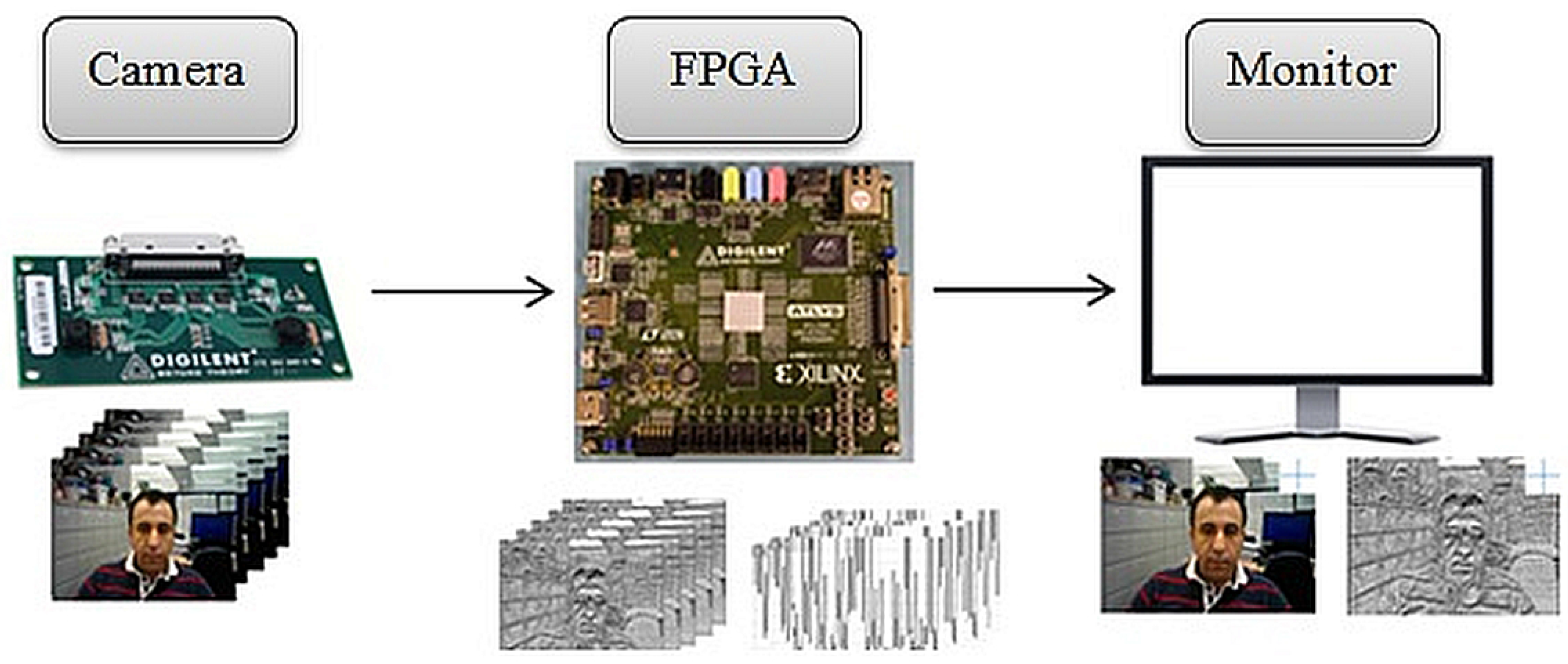
In the first part, the frames are extracted from the camera-sensor-captured video. The FPGA board that is used to implement the model is the Atlys™ Spartan-6 FPGA Development Board [40] along with a VmodCAM, Stereo Camera Module [41]. The Xilinx Spartan-6LX45 FPGA is used, which has a 128MB DDR2 RAM with 16 bit wide data. The Atlys™ board is intended for real-time video processing (see Figure 6). The VmodCAM is an additive device to the Atlys board. The Spartan-6LX45 FPGA sends commands and resolution settings to the VmodCAM through the I2C (Inter-Integrated Circuit) line. It contains a selection of clock, image colour and data settings.
In next section, the calculated LBP features are presented. To calculate, the images needed to be converted from RGB to grayscale; a Xilinx logiCORE IP RGB to YCrCb colour-space converter version 3.0 was used and fitted in the design. This is a basic 3 × 3 matrix multiplier changing three participation colours, which is 24 bits, to three output samples, which is 24 bits (8 bits for each element, Y, Cr and Cb) in only one clock period. In this work, only the 8 bits value of Y was used, which corresponded to the grayscale level of the input RBG. In MATLAB Simulink, as all frame pixels were available, therefore it was possible to process the LBP for the whole image in blocks of 3 × 3 pixels. On the other hand, as there was not enough RAM memory on the FGPA to save all the pixels of a single frame, we also aimed to have parallel LBP output; therefore, a row vector was used in the code to save 1283, which is equal to the first two rows’ pixel values plus three pixels from the third row. Therefore, we were required to wait until 1283 pixel values had been processed. As soon as the 1283 pixels were generated, then there was a block of 3 × 3 available to process the LBP algorithm. The pixel block will be moved through all the pixels and the values will be produced in a serial manner. Then the histogram can be generated for a whole image. This process would be carried on in the same way for all the pixels to the end. However, the camera sensor captured 30 frames per second with a resolution of 640 × 480; thus each pixel took 108.51 to be executed; therefore, there was a delay of 139.21 to produce the LBP pixel value. In order to wait for 1283 pixels to be ready, a delay was generated to do this. This would count the horizontal and vertical pixels, and all the RGB data for the 1283 pixels would be saved in an array to be accessed in the LBP processor; as soon as the third pixel in the third row was ready, the IP (Intellectual Property) library would be executed and would calculate and release the value of the pixel to the output. For the rest of the pixels, this process would be carried on in the same way for all the pixels to the end.
One of the main parts is the training datasets in the FPGA. A Xilinx LogiCORE IP Block Memory Generator version 6.2 is used to enter the features and labels into the model. In order to use this IP, the data has to be saved in a .coe file. The data should be all in one column (single data in each line) with a comma after each; the data can be input in integer or binary format. However, the largest data possible in the feature training dataset is 51256 in decimal notion; to represent it in the block memory generator, an IPCore of 16 bits width is needed, which limits and reduces the length of the data that can be used. This means that, with the 16 bits data width, there will be only 9999 lines available. However, to represent the feature in the .coe file, it is possible to have only one number in each line; on the other hand, as every 256 lines in the file is represented for one frame feature and only 9999 lines are available, therefore overall only 390 frames of data can be loaded to the IP. This is a disadvantage, as this will limit the model training datasets and will decrease the accuracy of the output.
The classification part using the k-NN algorithm on the training dataset contained the following maths operations: the power of 2 and the square root. On the other hand, in the Xilinx ISE Design Suite, there is no direct command to operate these two operations; there is only a command to multiply two numbers together. Therefore, to implement the k-NN algorithm, another two logiCORE IP Cores were used.
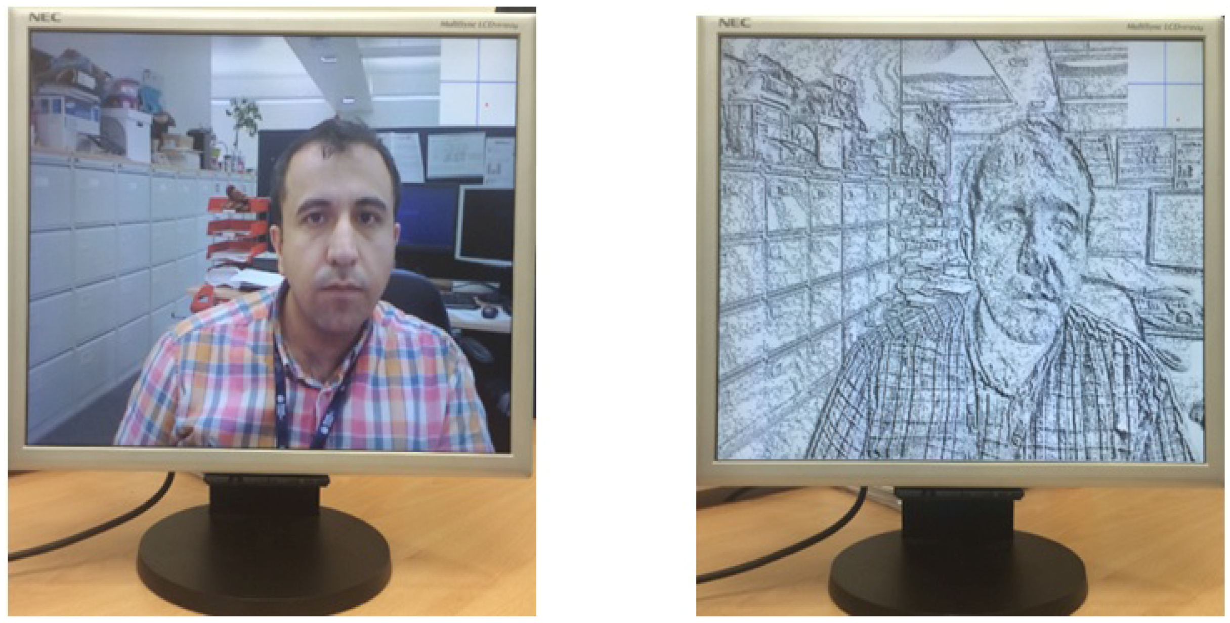
The fourth part is for displaying the predicted labels on the attached screen. When the model bit file downloaded to the FPGA board from the camera output, which is the live camera, can be seen on the monitor, the code has been modified to display the two-dimensional FeelTrace axis on the top-right corner of the monitor, with a white background and a resolution of 100 × 100 with blue axes. The horizontal axis indicates the valence and the vertical axis indicates the activation. The predicted label is displayed in a red colour; a box of 3 × 3 includes 9 pixels. One of the switches on the board is used in order to switch between both RGB and LBP view outputs, as shown in Figure 7.
5.5. Performance Comparison
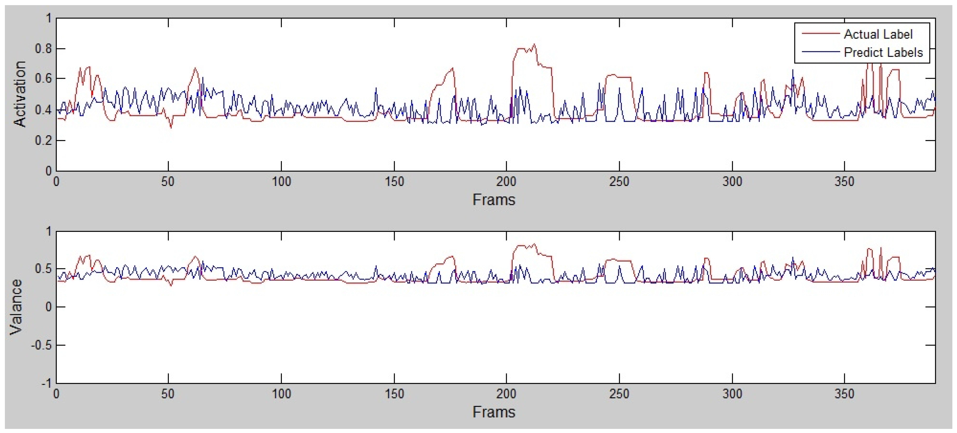
For cross-validating the results, 5- and 2-fold cross-validation were used. For the 5-fold person-independent (the system always contains the training data from more users) cross-validation, the captures were divided into five subsets. For the 2-fold cross-validation, always the second recording of the user went to testing (see example depicted in Figure 8).
The acquired accuracy of the system is depicted in Table 5 and Table 6. The highest accuracy was achieved for the 2-fold cross-validation for with an accuracy of 51.28% for MATLAB and 47.44% for the FPGA implementation.
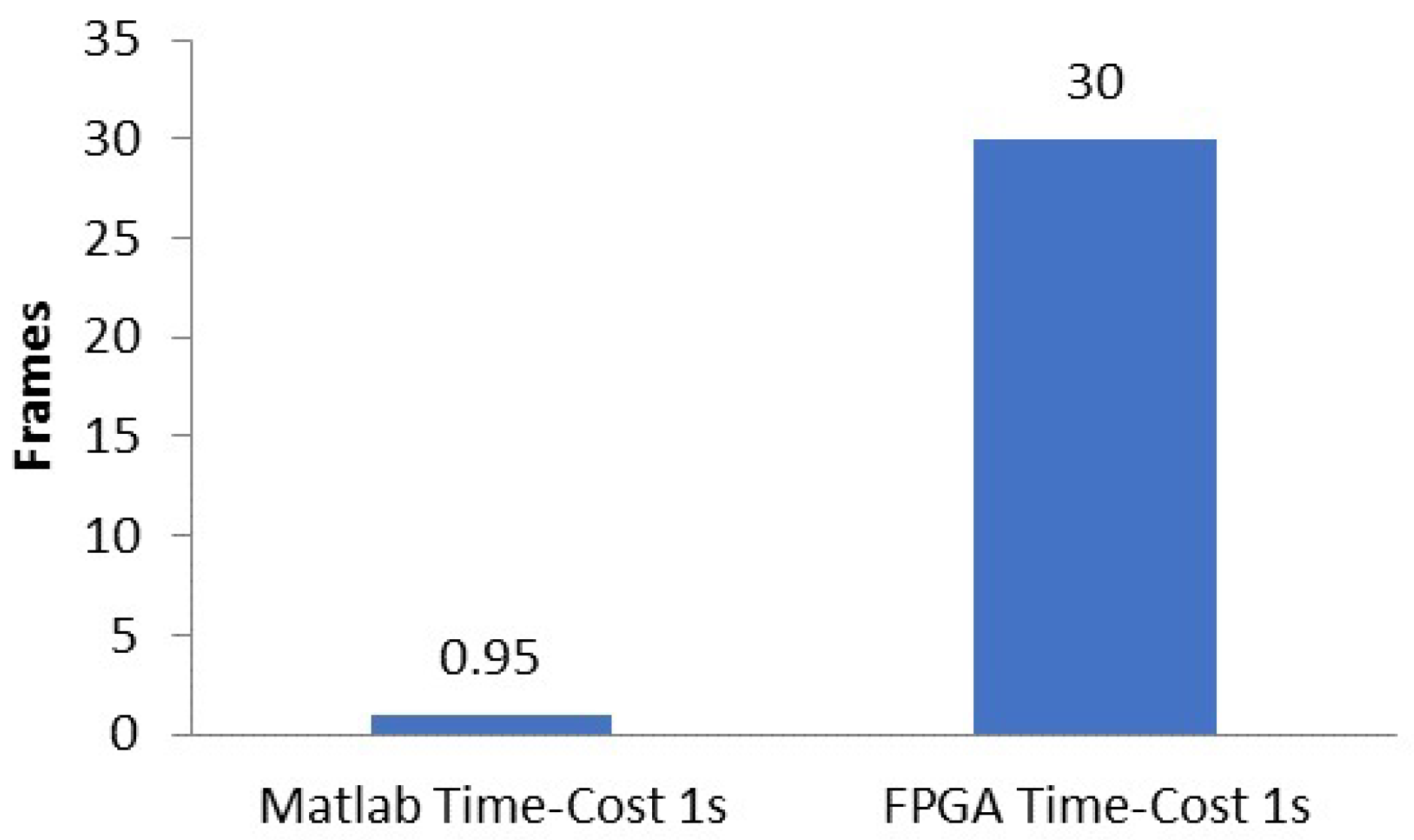
The accuracy of the predicted values was reduced for the FPGA by 3.84% compared to the MATLAB implementation, mainly because of the use of lower training datasets for the VHSIC (Very High Speed Integrated Circuit) Hardware Description Language (VHDL) implementation. The MATLAB Simulink code ran slower mainly because of the execution of the LBP algorithm and produced 0.95 frames every second. The FPGA implementation produced real-time outputs of 30 frames per second; therefore we conclude that it is more than 30 times faster compared to the MATLAB Simulink implementation, as depicted in Figure 9.
6. Conclusions and Discussion
The basis for the objective of this paper was to evaluate the FPGA implementation and efficiency of regression methods for automatic emotional state detection and analysis. It can be concluded that the results prove that the FPGA implementation is ready to be used on embedded devices for human emotion recognition from live cameras. The database of five users with 63,000 samples was recorded, labeled and cross-validated during the experiment. The LBP method was implemented for comparison in MATLAB and the FPGA. The values of the activation and valence for the database were extracted by FeelTrace from each frame.
The overall system accuracy of 47.44% is comparable with similar state-of-the-art work of J. Chen, conducted on the extended Cohn-Kanade (CK+) database (clean environment) and the Acted Facial Expression in Wild (AFEW) 4.0 database [42], with an overall average accuracy of 45.2% and between 0.6% for clean and 5% for “wild” videos for the accuracy achievement, and using a new proposed histogram of oriented gradients from three orthogonal planes (HOG-TOP) compared to LBP features used in this study for real-world videos (close to wild). The objective of this study was to appraise the efficiency of regression methods for automatic emotional state detection and analysis on embedded devices to be made on human emotion recognition from live cameras. A model was designed to process the emotional state using a collection of datasets for training and testing. These databases came from five recorded videos from five participants, each having been recorded twice. The LBP method was implemented to obtain the feature extraction of each video (frame-by-frame) by using MATLAB coding. The label database for each frame of the two emotions (activity and valence) were created using the FeelTrace definition and the GTrace application, which is an application to record emotions using a scoring system. For the regression modeling technique, the k-NN algorithm was utilized; then a model was designed and tested in MATLAB with 2- and 5-fold cross-validation with k-NN regression for different k values (1, 3 and 5). As seen in the implementation and results section, the best result belonged to the 2-fold cross-validation with for the k-NN algorithm.
In this study, MATLAB was used to test the model and find the best possible method that could be implemented on the available FPGA. A collection of video was needed to be recorded to build the model database, and this had to be obtained from the FPGA sensor camera (VmodCAM). The biggest challenge for this work was how to obtain the video data from the FPGA and save it; there was only 128MB of DDR2 RAM available on the FPGA board, and thus there was a limitation on saving the video data. Therefore, three different methods were implemented and tested on the two different boards:
- Receiving and saving the data in MATLAB Simulink via a universal asynchronous receiver/transmitter (UART) available on the board.
- Saving data on an SD card and implementing and testing on the Xilinx Spartan-6 FPGA Industrial Video Processing Kit.
- Connecting the HDMI output to a computer and using the MATLAB Acquisition application to record the video.
Finally, the third option was found as the best way to save the data.
To build a model in VHDL code, the Xilinx Spartan-6LX45 FPGA was used. The code that Digilent provided was used and modified extensively to meet the target specification. In this way, many different Xilinx LogiCORE IP’s were used. The output of the model is displayed at the top-right corner of a monitor with the participant’s live video. There is an option to view the RGB of the LBP view format of the video via a switch designed for this. It is possible to switch between these two at any time. As mentioned earlier, the best accuracy achieved in MATLAB Simulink was 51.28% and in the Xilinx simulation was 47.44%.
The system could be improved in the future work by using different deep learning algorithms; new feature extraction or different regression modeling methods such as SVR (Support Vector Regression), although difficult to design, have a proven potential to overcome the problems facing human emotion research today [37]. The results presented in this paper using a fusion system for automatic facial emotion recognition are promising. In the future, the audio features and speaker emotion detection models [43] will also be tested and fused [44] with the frame-level results.
Acknowledgments
We would like to thank Brunel Research Initiative & Enterprise Fund for financial support to the project entitled Automatic Emotional State Detection and Analysis on Embedded Devices. The research was supported partially by the Slovak Research and Development Agency under the research project APVV-15-0731. We also gratefully acknowledge the support of the NVIDIA Corporation with the donation of the Tesla K40 GPU used for this research.
Author Contributions
Saeed Turabzadeh was working as an MPhil. student on the face expression emotion analysis FPGA design and testing under supervisions of Hongying Meng and Rafiq Swash. Matus Pleva and Jozef Juhar were working on speech emotion analysis design together with Hongying Meng and gave advice and discussion for next steps, prepared the article, edition of the revisions, extend the state of art and results comparison with similar systems. All authors have read and approved the final manuscript.
Conflicts of Interest
The authors declare no conflict of interest.
References
- Ruta, D.; Gabrys, B. An Overview of Classifier Fusion Methods. Comput. Inf. Syst. 2000, 7, 1–10. [Google Scholar]
- Calder, A.J.; Young, A.W.; Perrett, D.I.; Etco, N.L.; Rowland, D. Categorical perception of morphed facial expressions. Vis. Cogn. 1996, 3, 81–117. [Google Scholar] [CrossRef]
- De Gelder, B.; Teunisse, J.-P.; Benson, P.J. Categorical perception of facial expressions: Categories and their internal structure. Cogn. Emot. 1997, 11, 1–23. [Google Scholar] [CrossRef]
- Miwa, H.; Itoh, K.; Matsumoto, M.; Zecca, M.; Takanobu, H.; Rocella, S.; Carrozza, M.C.; Dario, P.; Takanishi, A. Effective emotional expressions with expression humanoid robot WE-4RII: Integration of humanoid robot hand RCH-1. In Proceedings of the IEEE/RSJ International Conference on Intelligent Robots and Systems, Sendai, Japan, 28 September–2 October 2004; Volume 3, pp. 2203–2208. [Google Scholar]
- Turabzadeh, S.; Meng, H.; Swash, R.M.; Pleva, M.; Juhar, J. Real-time emotional state detection from facial expression on embedded devices. In Proceedings of the 2017 Seventh International Conference on Innovative Computing Technology (INTECH), Luton, UK, 16–18 August 2017; pp. 46–51. [Google Scholar]
- Darwin, C. The Expression of the Emotions in Man and Animals; Oxford University Press: Oxford, UK, 1998. [Google Scholar]
- Suwa, M.; Noboru, S.; Keisuke, F. A preliminary note on pattern recognition of human emotional expression. In Proceedings of the International Joint Conference on Pattern Recognition, Kyoto, Japan, 7–10 November 1978; pp. 408–410. [Google Scholar]
- Ekman, P.; Keltner, D. Universal facial expressions of emotion. Calif. Ment. Health Res. Dig. 1970, 8, 151–158. [Google Scholar]
- Picard, R.W.; Picard, R. Affective Computing; MIT press: Cambridge, MA, USA, 1997; Volume 252. [Google Scholar]
- Cheng, J.; Deng, Y.; Meng, H.; Wang, Z. A facial expression based continuous emotional state monitoring system with GPU acceleration. In Proceedings of the 2013 10th IEEE International Conference and Workshops on Automatic Face and Gesture Recognition (FG), Shanghai, China, 22–26 April 2013; pp. 1–6. [Google Scholar]
- Scherer, K.R. What are emotions? And how can they be measured? Soc. Sci. Inf. 2005, 44, 695–729. [Google Scholar] [CrossRef]
- Darwin, C. The Expression of Emotions in Man and Animals; Murray: London, UK, 1872; pp. 30 & 180. [Google Scholar]
- Ekman, P.; Friesen, W.V.; Hager, J.C. Facial Action Coding System The Manual. In Facial Action Coding System; Consulting Psychologists Press: Palo Alto, CA, USA, 2002; Available online: http://face-and-emotion.com/dataface/facs/manual/TitlePage.html (accessed on 23 November 2017).
- Fontaine, J.R.; Scherer, K.R.; Roesch, E.B.; Ellsworth, P.C. The World of Emotions is Not Two-Dimensional. Physiol. Sci. 2017, 18, 1050–1057. [Google Scholar] [CrossRef] [PubMed]
- Davidson, R.J.; Ekman, P.; Saron, C.D.; Senulis, J.A.; Friesen, W.V. Approach-withdrawal and cerebral asymmetry: Emotional expression and brain physiology: I. J. Pers. Soc. Psychol. 1990, 58, 330–341. [Google Scholar] [CrossRef] [PubMed]
- Stemmler, G. Methodological considerations in the psychophysiological study of emotion. In Handbook of Affective Sciences; Davidson, R.J., Scherer, K.R., Goldsmith, H., Eds.; Oxford University Press: Oxford, UK, 2003; pp. 225–255. [Google Scholar]
- Harrigan, J.; Rosenthal, R.; Scherer, K.R. The New Handbook of Methods in Nonverbal Behavior Research; Oxford University Press: Oxford, UK, 2005. [Google Scholar]
- Picard, R.W.; Klein, J. Computers that Recognise and Respond to User: Theoretical and Practical Implications. Interact. Comput. 2002, 14, 141–169. [Google Scholar] [CrossRef]
- Rajeshwari, J.; Karibasappa, K.; Gopalakrishna, M.T. S-Log: Skin based Log-Gabor Approach for Face Detection in Video. JMPT 2016, 7, 1–11. [Google Scholar]
- El Kaliouby, R.; Robinson, P. Real-time inference of complex mental states from facial expressions and head gestures. In Real- Time Vision for Human-Computer Interaction; Kisačanin, B., Pavlović, V., Huang, T.S., Eds.; Springer: Boston, MA, USA, 2005; pp. 181–200. [Google Scholar]
- Hernandez, J.; Hoque, M.E.; Drevo, W.; Picard, R.W. Mood Meter: Counting Smiles in the Wild. In Proceedings of the 2012 ACM Conference on Ubiquitous Computing, Pittsburgh, PA, USA, 5–8 September 2012; pp. 301–310. [Google Scholar]
- Meng, H.; Bianchi-Berthouze, N. Naturalistic affective expression classification by a multi-stage approach based on Hidden Markov Models. In Affective Computing and Intelligent Interaction. Lecture Notes in Computer Science; D’Mello, S., Graesser, A., Schuller, B., Martin, J.C., Eds.; Springer: Heidelberg, German, 2011; Volume 6975, pp. 378–387. [Google Scholar]
- Meng, H.; Romera-Paredes, B.; Bianchi-Berthouze, N. Emotion recognition by two view SVM_2K classifier on dynamic facial expression features. In Proceedings of the 2011 IEEE International Conference on Automatic Face & Gesture Recognition and Workshops (FG 2011), Santa Barbara, CA, USA, 21–25 March 2011; pp. 854–859. [Google Scholar]
- Cognitive Services. Available online: https://azure.microsoft.com/en-us/services/cognitive-services/ (accessed on 1 June 2017).
- Zhang, Y.D.; Yang, Z.J.; Lu, H.M.; Zhou, X.X.; Philips, P.; Liu, Q.M.; Wang, S.H. Facial Emotion Recognition based on Biorthogonal Wavelet Entropy, Fuzzy Support Vector Machine, and Stratified Cross Validation. IEEE Access 2016, 4, 8375–8385. [Google Scholar] [CrossRef]
- Wang, S.H.; Phillips, P.; Dong, Z.C.; Zhang, Y.D. Intelligent Facial Emotion Recognition based on Stationary Wavelet Entropy and Jaya algorithm. Neurocomputing 2018, 272, 668–676. [Google Scholar] [CrossRef]
- Cowie, R.; Douglas-Cowie, E.; Savvidou, S.; McMahon, E.; Sawey, M.; Schröder, M. ’FEELTRACE’: An instrument for recording perceived emotion in real time. In Proceedings of the ITRW on SpeechEmotion-2000, Newcastle, UK, 5–7 September 2000; pp. 19–24. [Google Scholar]
- Ahonen, T.; Hadid, A.; Pietikainen, M. Face description with local binary patterns: Application to face recognition. IEEE Trans. Pattern Anal. Mach. Intell. 2006, 28, 2037–2041. [Google Scholar] [CrossRef] [PubMed]
- Ojala, T.; Pietikäinen, M.; Mäenpää, T. Multiresolution gray-scale and rotation invariant texture classification with Local Binary Patterns. IEEE Trans. Pattern Anal. Mach. Intell. 2002, 24, 971–987. [Google Scholar] [CrossRef]
- Altman, N.S. An introduction to kernel and nearest- neighbor nonparametric regression. Am. Stat. 1992, 46, 175–185. [Google Scholar]
- Kohavi, R. A study of cross-validation and bootstrap for accuracy estimation and model selection. In Proceedings of the 14 International Joint Conference on Artificial Intelligence, San Mateo, CA, USA, 20–25 August 1995; pp. 1137–1143. [Google Scholar]
- Picard, R.; Cook, D. Cross-Validation of Regression Models. J. Am. Stat. Assoc. 1984, 79, 575–583. [Google Scholar] [CrossRef]
- Ojala, T.; Pietikainen, M.; Harwood, D. Performance evaluation of texture measures with classification based on Kullback discrimination of distributions. In Proceedings of the 12th IAPR International Conference on Pattern Recognition, Jerusalem, Israel, 9–13 October 1994; pp. 582–585. [Google Scholar]
- Jaskowiak, P.A.; Campello, R.J.G.B. Comparing correlation coefficients as dissimilarity measures for cancer classification in gene expression data. In Proceedings of the Brazilian Symposium on Bioinformatics, Brasília, Brazil, 10–12 August 2011; pp. 1–8. [Google Scholar]
- Pearson, K. Note on regression and inheritance in the case of two parents. Proc. R. Soc. Lond. 1895, 58, 240–242. [Google Scholar] [CrossRef]
- Cohen, J. Statistical Power Analysis for the Behavioral Sciences, 2nd ed.; Lawrence Erlbaum Associates: Hillsdale, NJ, USA, 1988. [Google Scholar]
- Turabzadeh, S. Automatic Emotional State Detection and Analysis on Embedded Devices. Ph.D. Thesis, Brunel University London, London, UK, August 2015. [Google Scholar]
- Chang, C.C.; Lin, C.J. LIBSVM: A library for support vector machines. ACM Trans. Intell. Syst. Technol. 2011, 2, 27. [Google Scholar] [CrossRef]
- The Linley Group. A Guide to FPGAs for Communications, 1st ed.; The Linley Group: Mountain View, CA, USA, 2009. [Google Scholar]
- Digilent Inc. AtlysTM Board Reference Manual. Available online: http://digilentinc.com/Data/Products/ATLYS/Atlys_rm.pdf (accessed on 11 July 2017).
- Digilent Inc. VmodCAMTM Reference Manual. Available online: http://digilentinc.com/Data/Products/VMOD-CAM/VmodCAM_rm.pdf (accessed on 30 June 2017).
- Chen, J.; Chen, Z.; Chi, Z.; Fu, H. Facial expression recognition in video with multiple feature fusion. IEEE Trans. Affect Comput. 2016. [Google Scholar] [CrossRef]
- Mackova, L.; Cizmar, A.; Juhar, J. A study of acoustic features for emotional speaker recognition in I-vector representation. Acta Electrotech. Inform. 2015, 15, 15–20. [Google Scholar] [CrossRef]
- Pleva, M.; Bours, P.; Ondas, S.; Juhar, J. Improving static audio keystroke analysis by score fusion of acoustic and timing data. Multimed. Tools Appl. 2017, 76, 25749–25766. [Google Scholar] [CrossRef]
Figure 1.
Video annotation process for valence using FeelTrace software. The video were shown on the left and the emotion labels were made by moving the mouse on the right.
Figure 1.
Video annotation process for valence using FeelTrace software. The video were shown on the left and the emotion labels were made by moving the mouse on the right.

Figure 2.
Real-time emotion detection system from facial expression on embedded devices.

Figure 3.
An example of an LBP histogram of an image. From one image, LBP algorithm can detect the angle or corner patterns of the pixels. Then a histogram on the patterns were generated.
Figure 3.
An example of an LBP histogram of an image. From one image, LBP algorithm can detect the angle or corner patterns of the pixels. Then a histogram on the patterns were generated.

Figure 4.
A high-level overview of the classifier system.

Figure 5.
Simulink data workflow diagram.

Figure 6.
Data workflow diagram and hardware used.

Figure 7.
Real-time display of the LBP feature implemented from FPGA hardware.

Figure 8.
Example of predicted and true valence and activation evaluation.

Figure 9.
Comparing computational costs of MATLAB and FPGA implementation.


Table 1.
Descriptions of facial muscles involved in the emotions Darwin considered universal [12].
Table 1.
Descriptions of facial muscles involved in the emotions Darwin considered universal [12].
| Emotion | Darwin’s Facial Description |
|---|---|
| Fear | Eyes open |
| Mouth open | |
| Lips retracted | |
| Eyebrows raised | |
| Anger | Eyes wide open |
| Mouth compressed | |
| Nostrils raised | |
| Disgust | Mouth open |
| Lower lip down | |
| Upper lip raised | |
| Contempt | Turn away eyes |
| Upper lip raised | |
| Lip protrusion | |
| Nose wrinkle | |
| Happiness | Eyes sparkle |
| Mouth drawn back at corners | |
| Skin under eyes wrinkled | |
| Surprise | Eyes open |
| Mouth open | |
| Eyebrows raised | |
| Lips protruded | |
| Sadness | Corner of mouth depressed |
| Inner corner of eyebrows raised | |
| Joy | Upper lip raised |
| Nose labial fold formed | |
| Orbicularis | |
| Zygomatic |
Table 2.
Cross-validation arrangement over the dataset.
| Cross Validation | |
|---|---|
| 5-Fold | 2-Fold |
Table 3.
Average Correlation Coefficient of Predicted Labels for 2- and 5-fold Cross-Validation.
| Average Correlation Coefficient | ||||
|---|---|---|---|---|
| 5-Fold | 2-Fold | |||
| k | Activation | Valence | Activation | Valence |
| 1 | 0.0226 | −0.0137 | 0.0561 | −0.0341 |
| 3 | 0.0260 | −0.0206 | 0.0713 | −0.0362 |
| 5 | 0.0294 | −0.0208 | 0.0785 | −0.0381 |
Table 4.
Average accuracy of confusion matrix for different k (MATLAB results).
| Accuracy (%) | ||
|---|---|---|
| 5-Fold | 2-Fold | |
| 1 | 27.66 | 45.82 |
| 3 | 28.13 | 49.47 |
| 5 | 27.77 | 51.28 |
Table 5.
Emotion detection accuracy achieved for different k of k-NN for MATLAB implementation.
| Accuracy (%) | ||
|---|---|---|
| 5-Fold (Person-Independent) | 2-Fold | |
| 1 | 27.66 | 45.82 |
| 3 | 28.13 | 49.47 |
| 5 | 27.77 | 51.28 |
Table 6.
Emotion detection accuracy achieved for different k of k-NN for FPGA implementation.
| Accuracy (%) | ||
|---|---|---|
| 5-Fold (Person-Independent) | 2-Fold | |
| 1 | 25.52 | 43.84 |
| 3 | 26.81 | 45.92 |
| 5 | 26.07 | 47.44 |
© 2018 by the authors. Licensee MDPI, Basel, Switzerland. This article is an open access article distributed under the terms and conditions of the Creative Commons Attribution (CC BY) license (http://creativecommons.org/licenses/by/4.0/).
Share and Cite
MDPI and ACS Style
Turabzadeh, S.; Meng, H.; Swash, R.M.; Pleva, M.; Juhar, J. Facial Expression Emotion Detection for Real-Time Embedded Systems. Technologies 2018, 6, 17. https://0-doi-org.brum.beds.ac.uk/10.3390/technologies6010017
AMA Style
Turabzadeh S, Meng H, Swash RM, Pleva M, Juhar J. Facial Expression Emotion Detection for Real-Time Embedded Systems. Technologies. 2018; 6(1):17. https://0-doi-org.brum.beds.ac.uk/10.3390/technologies6010017
Chicago/Turabian StyleTurabzadeh, Saeed, Hongying Meng, Rafiq M. Swash, Matus Pleva, and Jozef Juhar. 2018. "Facial Expression Emotion Detection for Real-Time Embedded Systems" Technologies 6, no. 1: 17. https://0-doi-org.brum.beds.ac.uk/10.3390/technologies6010017
Note that from the first issue of 2016, this journal uses article numbers instead of page numbers. See further details here.