Incremental and Multi-Task Learning Strategies for Coarse-To-Fine Semantic Segmentation


1
Department of Information Engineering, University of Padova, 35131 Padova, Italy
2
Higher School of Communication of Tunis (SupCom), Ariana 2083, Tunisia
*
Author to whom correspondence should be addressed.
Technologies 2020, 8(1), 1; https://0-doi-org.brum.beds.ac.uk/10.3390/technologies8010001
Submission received: 25 October 2019
/
Revised: 12 December 2019
/
Accepted: 13 December 2019
/
Published: 18 December 2019
(This article belongs to the Special Issue Computer Vision and Image Processing Technologies)
Abstract
:The semantic understanding of a scene is a key problem in the computer vision field. In this work, we address the multi-level semantic segmentation task where a deep neural network is first trained to recognize an initial, coarse, set of a few classes. Then, in an incremental-like approach, it is adapted to segment and label new objects’ categories hierarchically derived from subdividing the classes of the initial set. We propose a set of strategies where the output of coarse classifiers is fed to the architectures performing the finer classification. Furthermore, we investigate the possibility to predict the different levels of semantic understanding together, which also helps achieve higher accuracy. Experimental results on the New York University Depth v2 (NYUDv2) dataset show promising insights on the multi-level scene understanding.
1. Introduction
The semantic understanding of a scene is a long standing problem in the computer vision field that can be approached at different levels of interpretations. For instance, in image classification, a single label describing the main object in each image is returned as output. In object detection, instances of particular classes are identified by means of a bounding box which surrounds the objects and a label is assigned to each instance. Semantic segmentation, instead, is a dense labeling task in which a label has to be associated to each single pixel of the image. Similarly, we could interpret the scene at different levels of precision: In some scenarios, for example, it may be enough to identify just few classes while in others a more fine-grained prediction could be required. Moreover, in other settings, a coarse set of classes could be predicted first and then the set of classes could hierarchically grow into more refined categories to better understand the semantic context. To visualize this scenario, imagine an indoor navigation system first trained on a very coarse set of labels to segment, e.g. movable objects, permanent structures, and furniture, in order to, e.g., avoid obstacles. After a while, the dataset used for the initial training could be refined with a more fine-grained set of semantic classes (e.g., the movable objects class could be split into books, monitor, etc) and the task of the robotic system is to interact with these new types of objects. One solution could be to retrain from scratch the underlying neural network with the new set of classes; however, some other solutions may seem more reasonable. For instance, the initial prediction could be helpful for the learning process of the more refined set of classes in the form of an incremental learning approach where new tasks are accomplished at subsequent steps. Furthermore, solving multiple tasks at the same time could be beneficial in terms of both accuracy and the possibility to choose the appropriate set of labels for the particular task at hand (e.g., object avoidance, object interaction, etc.).
Starting from these considerations, the main goal of this work is to transfer previously gained knowledge, acquired on a simple semantic segmentation task with coarse classes (e.g., structures, furniture, objects, etc.), to a new model where more fine-grained and detailed semantic classes (e.g., walls, beds, cups, etc.) are introduced.
Notice that this task is similar to incremental learning; however, there are a few key differences. With respect to incremental learning for semantic segmentation [1], here we do not add the ability to segment and label new classes; instead, we refine the initial prediction on a coarse set of classes with a more fine-grained set of classes originated from the previous one. In this sense, indeed, we expand the ability of the deep neural network to accomplish the new fine-grained task.
The last focus of this work is the development of a new approach based on the simultaneous output of multi-level semantic maps. By exploiting domain sharing at the feature extraction level, the model will be fine-tuned to learn different levels of semantic labeling at the same time. This is somehow related to multitask learning [2,3,4], where multiple tasks are solved at the same time, while exploiting commonalities and differences across tasks. This can result in improved learning efficiency and prediction accuracy for the task-specific models, when compared to training the models separately. Training on multiple tasks could even bring additional information and, by sharing the representations between related tasks, we allow the model to generalize better on one or more tasks. Additionally, there is a reduction in the computational time with respect to training one independent architecture for each task. Our approach, however, is not strictly speaking multitask learning because we do not predict multiple different tasks at the same time (e.g., semantic maps along with depth information, surface normals, etc.) but actually we learn multiple sets of classes at the same time allowing to have different levels of representations of the semantic map simultaneously, greatly reducing the time required for the training (a single training replaces multiple steps of training). Furthermore, we share the same data across the tasks, which actually represent a different hierarchical clustering of the labels.
We based our approach on an end-to-end deep learning pipeline for semantic segmentation on color and depth data (i.e., color representation with an associated depth information) based on the DeepLab V3+ model [5]. To train the network and to evaluate the results, we employed the NYUDv2 dataset [6], which consists of a set of scenes of the indoor environment, with three sets of labels (5, 15 and 41 classes, respectively) at different levels of semantic precision and we compared our results with other recent methodologies, although not related to incremental or multitask approaches.
The remainder of this paper is organized as follows. Section 2 presents an overview of related work. In Section 3, the proposed methodologies are introduced. The employed dataset and training procedures are described in Section 4, while the experimental results are discussed in Section 5. Finally, Section 6 concludes our work and outlines some future developments.
2. Related Work
Semantic segmentation of a scene is a widely explored research problem that remains challenging despite the huge number of proposed approaches. It is one of the most challenging high-level tasks towards the direction of complete scene understanding and it is typically solved by means of deep learning approaches (see [7] for a recent review of the field). Most current state-of-the-art approaches are based on encoder–decoder schemes [8], on the Fully Convolutional Network (FCN) model [9,10], and on residual networks [11]. Some recent well-known and highly performing methods are DilatedNet [12], PSPNet [13], and DeepLab [14]. In particular, an enhanced version of the latter architecture, i.e., the Deeplab V3+ [5], is the architecture employed as starting point for this work.
Recently, due to the diffusion of consumer depth cameras, many datasets containing color and depth data have been created. In this work, we also exploit depth data and we adapt approaches for color images to this scenario with some modifications at the earlier layers. Although this work focuses more on the incremental refinement than at achieving high performance on the stand-alone segmentation task, a brief overview of recent research papers is presented here. In [15,16], a scheme involving CNN at multiple scales has been adopted. Two different CNNs for color and depth and a feature transformation network are exploited in [17]. In [18], a region splitting and merging algorithm for RGB-D data has been proposed. In [19], a MRF superpixel segmentation is combined with a tree-structured segmentation for scene labeling. Multiscale approaches have also been exploited (e.g., [20]). Hierarchical segmentation based on the output of contour extraction has been used in [21], which also deals with object detection from the segmented data. Another combined approach for segmentation and object recognition has been presented in [6], which exploits an initial over-segmentation followed by a hierarchical scheme.
The problem of knowledge transfer in machine learning was first introduced by Bucilua et al. [22] in 2006. They focused on the idea of compressing whole ensemble of models (a collection of models whose final predictions are averaged) into a single and simpler model that is easier and faster to train. This concept was further developed in [23], where the authors tried to solve the problem of adding new classes without losing the model’s performance on the older set of classes introducing the idea of knowledge distillation.
Knowledge distillation and incremental learning techniques have not yet been considerably exploited in the task of semantic image segmentation; indeed, previous studies mainly focus on classification and recognition tasks. One of the first works dealing with incremental learning in the semantic segmentation task is [1,24], where the authors applied knowledge distillation to preserve old classes while incrementally enlarging the capabilities of the learning architecture to properly segment and label new sets of classes. However, the task presented here is considerably different in that all the training images are available from the beginning and the sets of labels are progressively split into more fine-grained hierarchical categories and then revealed to the learner.
The last idea we want to investigate is the multiple learning of more representations at the same time, which is somehow related to multitask learning [2,3,4]. Multitask learning has been widely applied to semantic segmentation. For instance, in [16], a single multiscale CNN is employed to solve the three tasks of depth prediction, surface normals estimation, and semantic labeling. In [25], the semantic segmentation task is solved using three networks with shared features: Differentiating instances, estimating masks, and categorizing objects. In [26], multitask learning is employed to align the features computed from synthetic data while performing the predictions of the depth, the edges, and the surface normals with the ones computed from real-world images. In [27], the semantic segmentation map is predicted together with instance segmentation and depth prediction; additionally, an approach to select the weights for each loss is proposed.
3. Proposed Methods
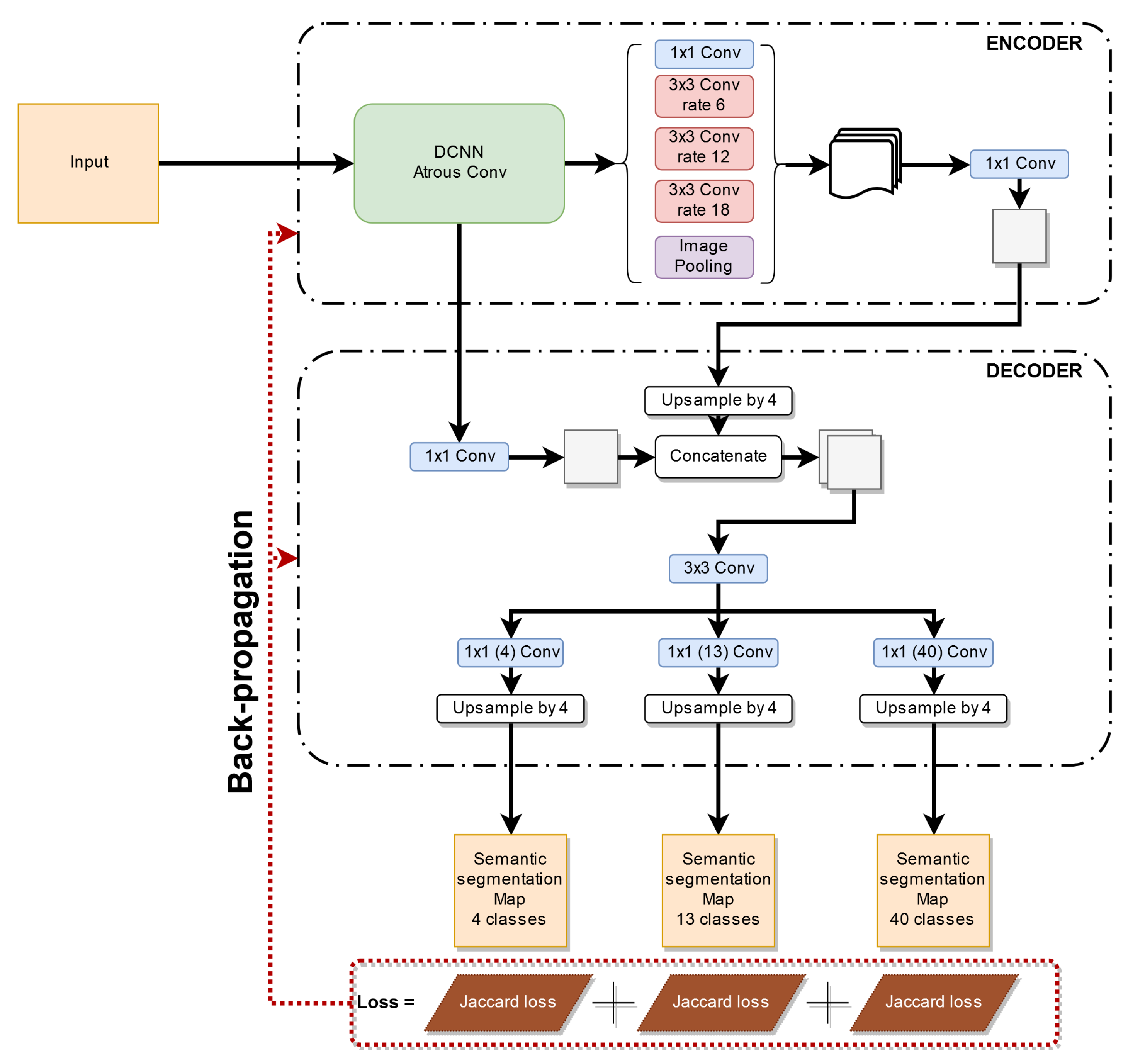
In this section, we show in detail the approaches proposed in this work. Although the proposed procedures are agnostic to the underlying architecture, for the evaluation, we chose the Deeplab V3+ [5,14] network, which has state-of-the-art performance on segmentation tasks. The network consists of a Xception feature extractor, whose weights were pre-trained [28] on the Pascal VOC 2012 dataset [29], and a decoder made by Atrous Spatial Pyramid Pooling (ASPP) layers. We evaluated our results on the NYUDv2 dataset after a pre-processing stage detailed in Section 4.
As with most deep learning approaches, the model takes as input a multi-channel tensor (in our case, nine channels corresponding to the color image, the depth information and the surface normals) and outputs the predicted softmax tensor with a number of channels equal to the number of predicted classes. This operation returns a probability distribution containing for each pixel the probability of belonging to each specific class. The class corresponding to the highest probability value is chosen for each pixel by an argmax operation. As a final result, we end up with the predicted segmentation map where each pixel value is the index of the class it belongs to.
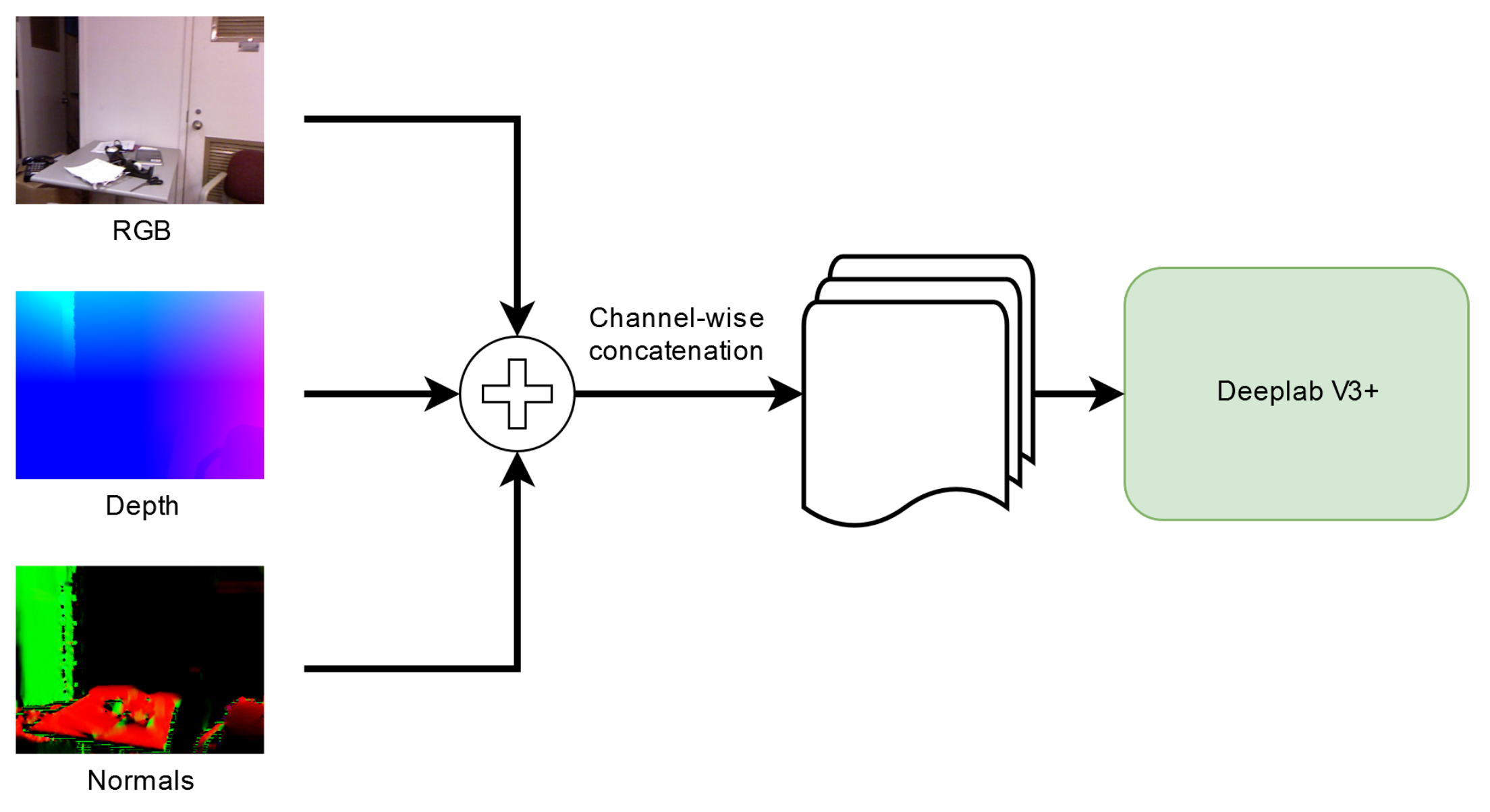
To exploit the multiple types of information, we performed an early fusion of the different representations, i.e., color, depth, and surface normals, as depicted in Figure 1, and then we feed them to the network. More in detail, each input tensor has nine channels. The first three channels correspond to the RGB color representation in the range , i.e., we divided by 127.5 the color values and then subtracted 1. The following three channels correspond to the geometry components where each channel represents the position of each pixel with respect to the three axes (X,Y,Z) of the 3D space. We normalized these values by subtracting the mean and dividing by the standard deviation along each axis. The last three channels represent the surface normal vectors. We used the standard representation with the three components of the unit vector perpendicular to the surface at each location (i.e., the components assume values in the range and the vector norm is equal to 1).
For the training procedures, we employed the Jaccard loss (also known as Intersection over the Union (IoU) loss). We chose this loss since it has proven to be useful when training on a dataset with unbalanced numbers of pixels in the different classes within an image because it gives equal weight to all classes. Additionally, it has shown better perceptual quality than the usual cross-entropy loss with our setup in which there are some small objects and many under-represented labels in the dataset. The Jaccard loss is defined as:
where represents the cardinality of the considered set, is the predicted segmentation map, and y is the ground-truth map.
3.1. Hierarchical Learning
In this section, we present and discuss the various methods we designed for knowledge transfer in semantic segmentation.
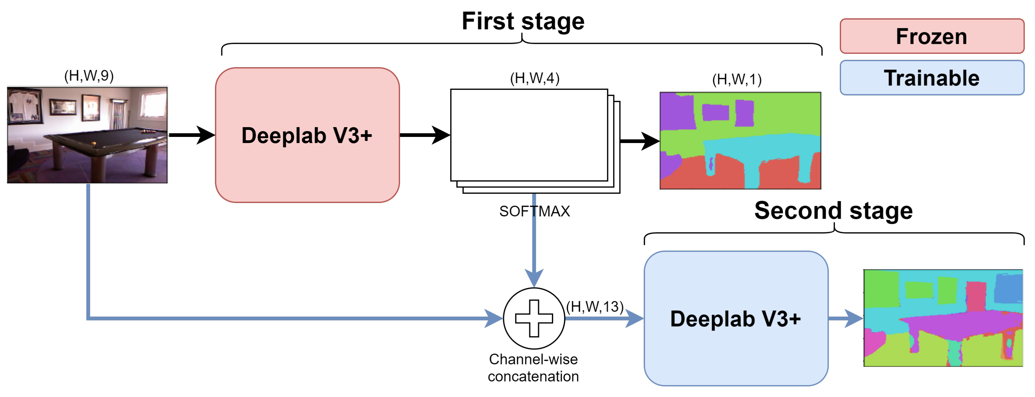
In the first approach, we used a different Deeplab V3+ model for each step (i.e., on the considered dataset, we have a first model for the 5-class setting, a second for the 15-class setting, and a third for the 41-class setting). As every incremental learning approach, we start by training the Deeplab V3+ model on the coarser set of classes (e.g., five classes in our scenario). After that, we freeze the first model and we employ its output of the softmax operation as an additional input component when we train the model on the set of more fine-grained classes (e.g., 15 classes). We repeat the same approach also when moving from to (i.e., from 15 to 41 classes). This methodology was partially derived by the idea presented in [18] where the softmax information is used for binary classification task. Furthermore, notice that, when training for the finer tasks, the networks corresponding to the coarser ones are frozen, i.e., we do not train in a single step a large size network containing the two (or three) networks for the two (or three) tasks but we perform a set of independent trainings each working on a single stage of the network.
More in detail, the number of predicted classes were 4, 13 and 40, respectively, because the unknown and the unlabeled classes were discarded as done by all competing approaches (see Section 4 for further details). Note that the number of trainable parameters remains constant during the two stages because in the incremental step the previous network is completely frozen and not trained anymore. The proposed framework is shown in Figure 2 and it is evident that the previous stage of training acts as a conditioning element for the following one. Indeed, the softmax tensor output from the first training stage (i.e., from ) serves as additional input (concatenating it with the RGB images) for the second stage (model ) and the same idea is exploited when moving from to . This way the network is constrained to learn the mapping from the coarser to the finer-grained sets of classes.
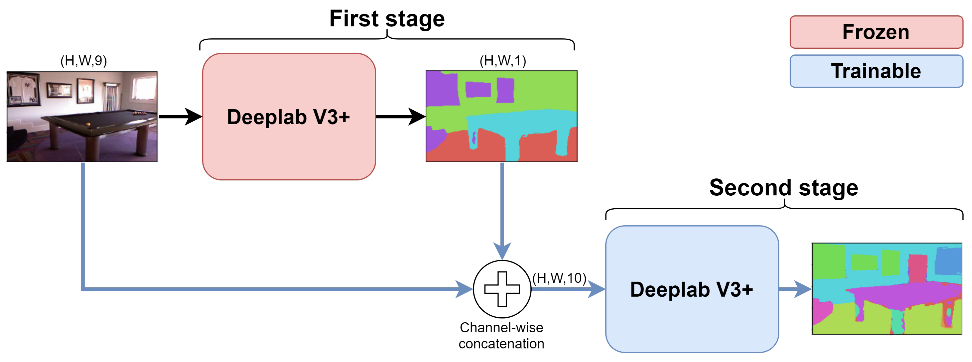
In the second approach, we fed as an additional input to the incremental stages the argmax of the predicted semantic map instead of the softmax. This approach is shown in Figure 3. The main difference from previous approach is that we only feed the index of the maximum of the predicted map and we drop the information about the probabilities of all the various classes which was before represented by the softmax vector for each pixel. In this way, we lose the information about the uncertainty of the prediction but, on the other side, the representation is much more compact having only a single value representing the predicted class for each pixel. Notice that the first approach (softmax) is more complex but leads to slightly better results (see the experimental evaluation in Section 5). On the other side, the second approach (argmax) is faster and simpler even if it has slightly worse performance.
In the third approach, we fed as additional input to the incremental stages the edges of the predicted semantic map. This approach is shown in Figure 4. Differently from before, the additional information channel does no longer contains the semantic labels of the classes but instead is represented by the boundary information. In this way, the second stage of training is more focused on the contours of the shapes, which are generally difficult to discriminate in semantic segmentation tasks.
We argue that combining multiple cues could lead to further improvements; however, this possibility is limited in practice by memory constraints of the employed GPUs.
3.2. Joint Learning of Multiple Representations
Finally, we started to investigate the prediction of different labelings at the same time and whether this could be helpful to improve performance on the coarser set of labels since we are learning more detailed information about their content and vice versa if the coarse labeling can help the fine one. We then designed a different decoder to accomplish the multiple representations and we trained the architecture end-to-end with three different losses (one for each set of labels). In this case, the complete loss function is defined as:
where is the ith set of labels, i.e., , , and contain, respectively, 5, 15, and 41 classes, while the hyper-parameters balance the three losses. They were empirically set to 1 so that all the terms contribute equally during the back-propagation phase. The loss associated with the set is then written as . The approach is illustrated in Figure 5: We used a single standard DeepLab V3+ encoder while the decoder has been modified to be able to deal with the multiple tasks together. From this figure, we can appreciate that the first part of the decoder is shared across all the tasks while the last convolution layer is unique for each segmentation task (i.e., 4, 13, and 40 classes segmentation in our case, after excluding the unknown and the unlabeled classes as detailed in Section 4). The final layers are followed by a bilinear upsampling procedure to restore the original input dimensions and a softmax classification layer is then applied to each output to get the final predictions.
4. Training on the NYUDv2 Dataset
The NYUDv2 dataset [6] was used to train the proposed architectures and to evaluate the performance of the proposed approach. This dataset contains 1449 depth maps and color images of indoor scenes acquired with a first generation Kinect sensor divided into a training set with 795 scenes and a test set with the remaining 654 scenes. The original resolution of the images is ; however, for the training procedures, we employed a lower resolution of for memory constraints. The evaluation of the results, instead, was carried out on the original resolution images for a fair comparison with competing approaches. For results evaluation, we used the ground truth labels from [30], and we considered the three clusters of 5, 15, and 41 labels, respectively, as mapped in [6,31].
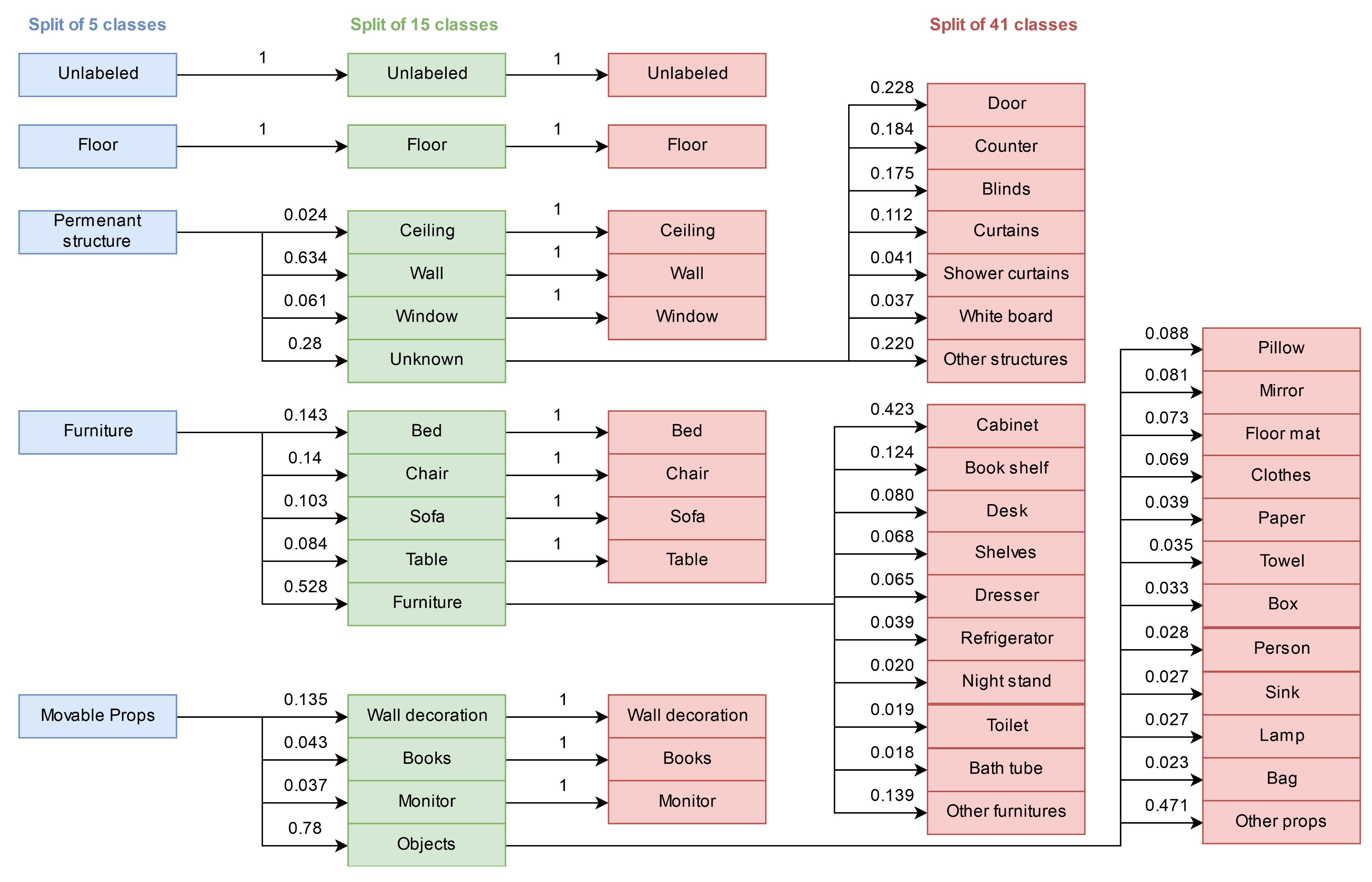
In particular, the three considered set of labels are hierarchically represented in Figure 6 where we can appreciate how the derived classes emerge from parent ones. Two classes, i.e., unlabeled and floor, are peculiar because they are never split when moving to finer semantic representations. Similarly, various classes in the set of 15 labels are not split when moving to the finer set of 41. From the diagram, we can notice how there are clear unbalanced splitting situations. For instance, some classes of the split of 15 are underrepresented in the dataset, as can be appreciated from the very low fraction of pixels in these classes from parent ones: e.g., ceiling and window are present in only and , respectively, of instances of permanent structure; and monitor and books are derived only in the and of the movable props parent class. Additionally, the splitting is not uniformly distributed among the parent classes, thus from 3 out of 5 classes of the split of 5 derive 13 out of 15 classes of the split of 15. If we move to the analysis of the split of 41, the considerations become even more severe. There are few classes deriving from of instances of parent class, e.g. bath tub, toilet, night stand, and many others (10 classes) deriving from 2–5%. Moreover, it should be noticed that, in this case, 29 classes out of 41 derive from just three parent classes, thus confirming the extreme inhomogeneity of this splitting.
As done by all the competing approaches (e.g., [16,18,31,32]), we removed both from the prediction and from the evaluation of the results the unlabeled and unknown classes when present. Indeed, they are fictitious classes artificially created during the labeling procedures of the images. This choice allowed directly comparing the results with competing approaches, although not related to incremental or multi-tasking learning.
Moreover, in Figure 7, we can appreciate the various level of semantic understanding which have been considered for the evaluation. For instance, in the first row, we can visualize how the generic furniture class in the set of five classes (in yellow) is split into bed and furniture in the set of 15 classes (light blue and blue, respectively) and that bed is further refined into bed and pillows in the set of 41 classes (in orange and light green, respectively). Again, in the second row, for example, we can appreciate how the generic class movable props of the set of five classes (in purple) is then refined to books and object in the set of 15 classes (in dark green and light purple, respectively), and then further refined in the last set of classes. Finally, in the third row, we can visualize how the permanent structure class in the set of five classes (in orange) is then split into the classes ceiling and wall in the set of 15 classes (in yellow and pink, respectively).
The various approaches were trained on the NYUDv2 training set using the three different sets of labels. We employed Stochastic Gradient Descent (SGD) and ran the procedure for 100 epochs. The initial learning rate was set to , the weight decay to , and the batch size equal to 2. The learning rate scheduler decreased the learning rate every epochs using the following formula:
where ep denotes the index of the current epoch.
We used TensorFlow [33] to develop and train our framework. For each stage, the number of trainable parameters and FLOPs was roughly the same as the original Deeplab V3+ architecture, i.e., 41M and 82B, respectively (the added components require a very small number of parameters with respect to the Deeplab model). The training of the neural network took about 22 h on a NVIDIA Tesla K40 GPU with Intel(R) Core(TM) i7 CPU 970 @ 3.2 Ghz. The implementation of the proposed model is available at https://github.com/LTTM/IL-Coarse2Fine.
5. Experimental Results
In this section, we discuss the performance of the various proposed approaches in the two different settings of incremental and multi-task learning.
First, we start by comparing our modified Deeplab V3+ architecture with early fusion of the three information representations, i.e., color, depth, and surface normals, with some recent works. To evaluate the results, we employed the most widely used metrics for semantic segmentation problems: The Pixel Accuracy (PA), the mean Class Accuracy (mCA), and the mean Intersection over Union (mIoU) [34].
The modified network is able to obtain state-of-the-art results on all the three set of labels. In Table 1, we can confirm that our baseline network could outperform competing approaches in terms of both PA and mCA on the split of four classes; additionally, we also show the obtained mIoU. Similar results were achieved by our baseline model for the set of 13 classes, as shown in Table 2, while on the set of 40 labels some very recent approaches have better performance (see Table 3). However, notice that the aim of this work is to propose an efficient hierarchical learning strategy, not to improve the performance on the segmentation task by itself.
Then, we evaluated our hierarchical learning approaches. Firstly, we started from the coarser set of four classes and we moved to the prediction of 13 classes: The results are shown as the last three lines of Table 2 for the three different approaches. In this case, we can appreciate that the addition of the softmax information from the four-class model or of the edges information are useful cues to reach higher accuracy on the new set of classes if compared with the baseline counterpart. In particular, in the case of softmax or edges information, there are improvements in all three considered metrics with respect to the baseline Deeplab V3+. In particular, the softmax information leads to the best class accuracy (almost ) while the use of edge information is the best strategy with respect to the pixel accuracy () and to the mIoU (). Notice that the mIoU gap with respect to the direct training on the 13 classes is about (by the way, this metric and the mCA are more interesting for our task since the pixel accuracy is strongly dependent on large structures such as the floor that are not split in the hierarchical labeling). The argmax information, instead, brings a limited contribution to the final accuracy values.
One may argue what would happen if we train both the first and the second stage with the same set of classes (i.e., by just using a deeper network without really exploiting the hierarchical structure of the classes). We expect this scenario to achieve almost the same results of our baseline approach, or slightly higher, since we are retraining the same architecture with an additional input, which is the output of the previously trained network. At the same time, we expect that the incremental framework is the dominant factor for the performance increase. Indeed, the results for this stacking are perfectly in line with our intuition, as reported in Table 2 with the name “Stacking”.
Furthermore, we performed an additional incremental step to predict the set of 40 classes starting from the prediction of the set of 13 labels. The results are reported in Table 3. In this case, our method was outperformed by some methods in the literature, due to some inner limitations of the employed Deeplab V3+ architecture. However, the most interesting thing for this work is the comparison with our baseline method, i.e., Deeplab V3+ directly trained on the 40 classes, in order to appreciate the gain of the hierarchical approaches.
We can appreciate how the three additional cues employed produce some improvements in the various metrics even if the gain is more limited. The result is still noticeable if we remember that the splitting is highly unbalanced and inhomogeneous as we have seen in Section 4.
Finally, in Table 4, we evaluate our joint learning approach on the three sets of classes simultaneously. We can appreciate that the joint model allows not only to predict the three sets of labels at the same time, without the need for multiple training stages, but also to improve the accuracy with respect to the baseline in all the scenarios and for all the metrics. The improvement, although consistent across all experiments and metrics, is sometimes modest and smaller than some of the previously proposed methods. The highest gains are achieved in the PA and mIoU for the set of four classes and in the PA for the set of 40 classes. It should be noticed that the chosen architecture is already highly performing, especially on the sets of 4 and 13 classes.
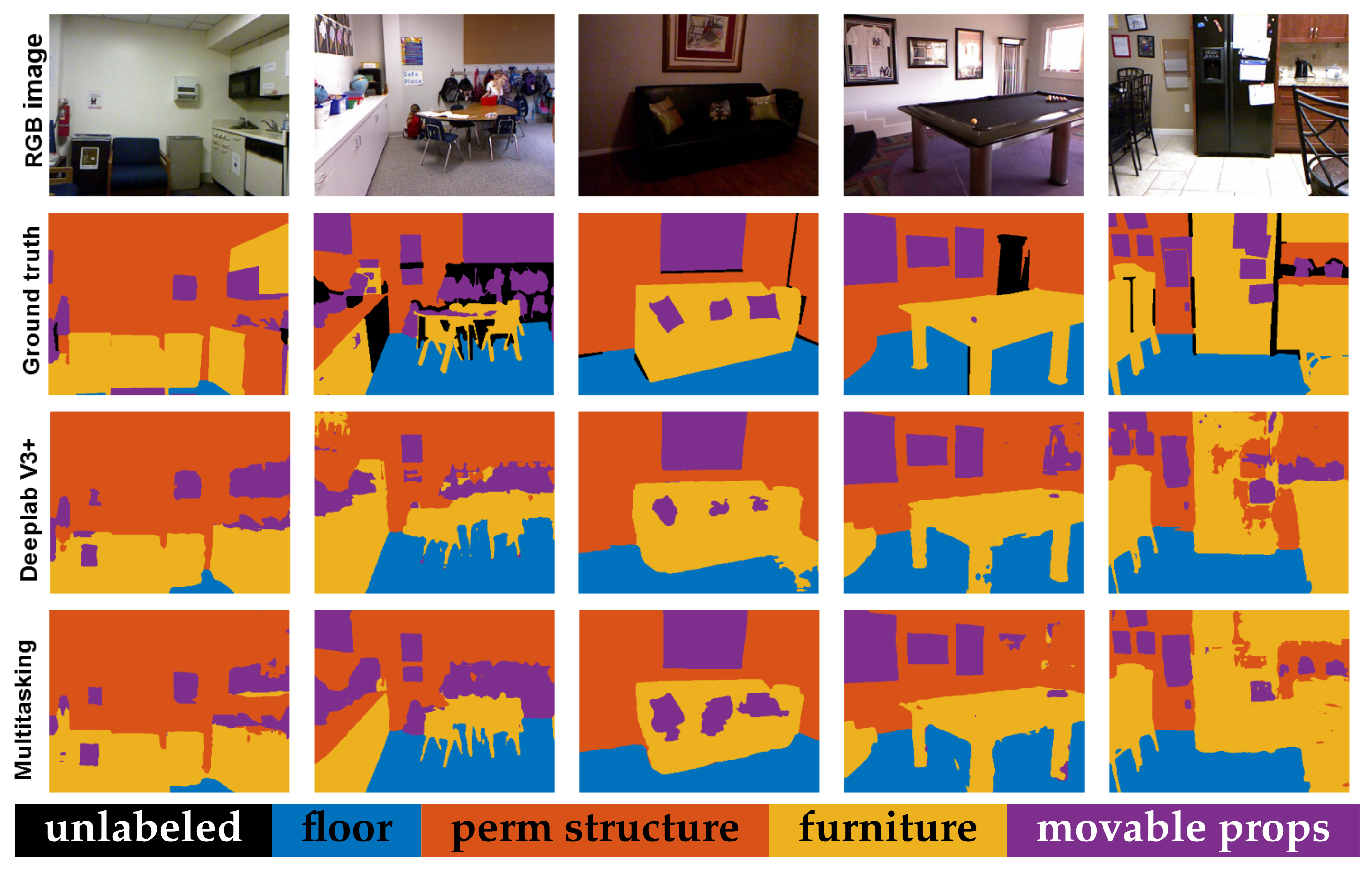
Figure 8 shows some qualitative results for the set of five classes. Here, we can compare the performance of our baseline Deeplab V3+ with respect to the multi-tasking approach (the other methods do not apply to this setting since there is no coarser representation). As already noticed, both the approaches have very high accuracy on this task. The image in the first column is very similar between the two approaches; however, we can verify how the multi-tasking learning outperforms the baseline in the remaining four images. In particular, look at the purple object on the top left of the figure in second column, the orange top of the furniture on the left, or again to the purple objects on the center-right of the image. In Column 3, we can clearly see an improvement in the definition of the shapes of the sofa and of the pillows. Similarly, the wall and the furniture are better recognized in the last two images.
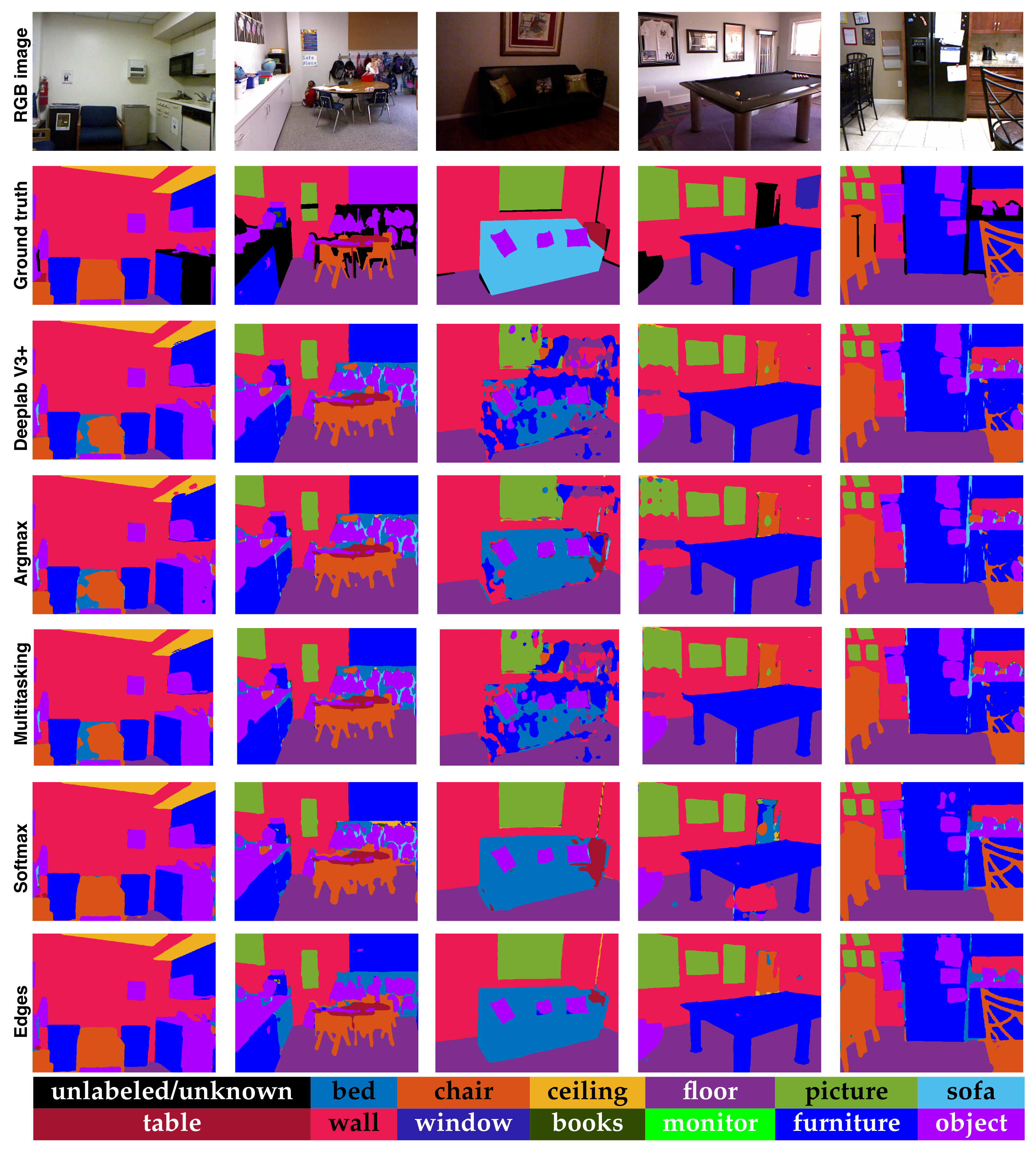
Finally, we report in Figure 9 the qualitative results for the split of 15 classes for all the proposed approaches. From the figure, we can appreciate that the incremental approach with the softmax or the edges generally lead to a much cleaner prediction with few artifacts. This can be seen particularly well in Column 1, where the chair in the center of the image is fully recovered by the proposed incremental methods, and in Column 3, where the wall is cleaned from prediction errors (in this scene, the sofa has also been properly segmented but a wrong label of bed has been associated to it). In the same scenes, the baseline, the incremental approach with the argmax, and the multi-tasking suffer from some artifacts. In Column 4, we can notice that the edges information revealed to be more significant than the softmax information to properly recognize the leg of the pool table.
In general, we argue that the incremental approaches with edges or softmax information are much more reliable than the conditioning based on the argmax: In the softmax case, a larger amount of information is fed as additional input giving the network the possibility to discriminate between certain or uncertain predictions while in the edges case the network is forced to focus more on the edges of the objects, which typically represent one of the most challenging characteristics to be learned.
For what concern computational requirements, the inference time of the modified Deeplab V3+ network is 23 ms on the workstation used for the training (with an Intel 970 CPU and a Nvidia K40 GPU), which is roughly the same as the standard DeepLab V3+ architecture. Notice that incremental schemes require multiple inferences, e.g., the 13 classes experiment requires executing the model two times in cascade (one for the four-class network and one for the 13-class network taking in input also the outcome of the four-class model). If real-time performance were needed, the best option would be the joint learning scheme proposed in Section 3.2 that is able to perform all three tasks with a single pass through the encoder module that is the most computationally demanding stage being the decoder very lightweight. As a comparison, current works (e.g., [37,38]) report a higher computation time of s and 78 ms, even if a direct comparison is not possible due to the completely different hardware setups.
6. Conclusions
In this paper, we introduce and address the novel problem of hierarchical incremental learning where a first deep neural network is trained on a small set of macro-classes and is then adapted and refined to recognize a larger set of classes with a finer semantic content. We propose three different hierarchical strategies exploiting the softmax and argmax of the coarse network output and the edges information from the segmentation maps of the coarse network. Furthermore, a scheme for the joint training on the three tasks is also proposed. Experimental results show that all the proposed schemes allow improving the performance with respect to the direct training on the larger set of classes.
Further research will be devoted to improving the multitask approach, eventually also with the addition of different tasks (e.g., the prediction of the surface normals or of the depth maps without using them as inputs). Given that the proposed methodologies are agnostic to the underlying neural network architecture, we will consider employing a more lightweight network that allows combining multiple cues together.
Author Contributions
Conceptualization, M.M., U.M., and P.Z.; Methodology, M.M., U.M., and P.Z.; Software, M.M.; Supervision, U.M. and P.Z.; Writing—original draft, U.M.; and Writing—review and editing, M.M. and P.Z. All authors have read and agreed to the published version of the manuscript.
Funding
This research received no external funding.
Acknowledgments
We gratefully acknowledge the support of the NVIDIA Corporation with the donation of one NVIDIA K40 GPU for our research.
Conflicts of Interest
The authors declare no conflict of interest.
References
- Michieli, U.; Zanuttigh, P. Incremental Learning Techniques for Semantic Segmentation. In Proceedings of the International Conference on Computer Vision Workshops (ICCVW), Seoul, Korea, 27 October–2 November 2019. [Google Scholar]
- Thrun, S. Is learning the n-th thing any easier than learning the first? In Proceedings of the International Conference on Neural Information Processing Systems (NeurIPS), Denver, CO, USA, 2–5 December 1996; pp. 640–646. [Google Scholar]
- Baxter, J. A model of inductive bias learning. J. Artif. Intell. Res. 2000, 12, 149–198. [Google Scholar] [CrossRef]
- Caruana, R. Multitask learning. Mach. Learn. 1997, 28, 41–75. [Google Scholar] [CrossRef]
- Chen, L.C.; Zhu, Y.; Papandreou, G.; Schroff, F.; Adam, H. Encoder-Decoder with Atrous Separable Convolution for Semantic Image Segmentation. In Proceedings of the European Conference on Computer Vision (ECCV), Munich, Germany, 8–14 September 2018; pp. 833–851. [Google Scholar]
- Silberman, N.; Hoiem, D.; Kohli, P.; Fergus, R. Indoor segmentation and support inference from RGBD images. In Proceedings of the European Conference on Computer Vision (ECCV), Florence, Italy, 7–13 October 2012. [Google Scholar]
- Garcia-Garcia, A.; Orts-Escolano, S.; Oprea, S.; Villena-Martinez, V.; Martinez-Gonzalez, P.; Garcia-Rodriguez, J. A survey on deep learning techniques for image and video semantic segmentation. Appl. Soft Comput. 2018, 70, 41–65. [Google Scholar] [CrossRef]
- Badrinarayanan, V.; Kendall, A.; Cipolla, R. SegNet: A Deep Convolutional Encoder-Decoder Architecture for Image Segmentation. IEEE Trans. Pattern Anal. Mach. Intell. (TPAMI) 2017, 39, 2481–2495. [Google Scholar] [CrossRef] [PubMed]
- Long, J.; Shelhamer, E.; Darrell, T. Fully convolutional networks for semantic segmentation. In Proceedings of the IEEE Conference on Computer Vision and Pattern Recognition (CVPR), Boston, MA, USA, 7–12 June 2015; pp. 3431–3440. [Google Scholar]
- Shelhamer, E.; Long, J.; Darrell, T. Fully Convolutional Networks for Semantic Segmentation. IEEE Trans. Pattern Anal. Mach. Intell. (TPAMI) 2016, 39, 640–651. [Google Scholar] [CrossRef] [PubMed]
- Lin, G.; Milan, A.; Shen, C.; Reid, I. Refinenet: Multi-path refinement networks for high-resolution semantic segmentation. In Proceedings of the IEEE Conference on Computer Vision and Pattern Recognition (CVPR), Honolulu, HI, USA, 21–26 July 2017. [Google Scholar]
- Yu, F.; Koltun, V. Multi-scale context aggregation by dilated convolutions. In Proceedings of the International Conference on Learning Representations (ICLR), San Juan, Puerto Rico, 2–4 May 2016. [Google Scholar]
- Zhao, H.; Shi, J.; Qi, X.; Wang, X.; Jia, J. Pyramid scene parsing network. In Proceedings of the IEEE Conference on Computer Vision and Pattern Recognition (CVPR), Honolulu, HI, USA, 21–26 July 2017; pp. 2881–2890. [Google Scholar]
- Chen, L.C.; Papandreou, G.; Kokkinos, I.; Murphy, K.; Yuille, A.L. Deeplab: Semantic image segmentation with deep convolutional nets, atrous convolution, and fully connected crfs. IEEE Trans. Pattern Anal. Mach. Intell. (TPAMI) 2018, 40, 834–848. [Google Scholar] [CrossRef] [PubMed]
- Couprie, C.; Farabet, C.; Najman, L.; Lecun, Y. Convolutional nets and watershed cuts for real-time semantic Labeling of RGBD videos. J. Mach. Learn. Res. (JMLR) 2014, 15, 3489–3511. [Google Scholar]
- Eigen, D.; Fergus, R. Predicting depth, surface normals and semantic labels with a common multi-scale convolutional architecture. In Proceedings of the International Conference on Computer Vision (ICCV), Santiago, Chile, 7–13 December 2015; pp. 2650–2658. [Google Scholar]
- Wang, J.; Wang, Z.; Tao, D.; See, S.; Wang, G. Learning Common and Specific Features for RGB-D Semantic Segmentation with Deconvolutional Networks. In Proceedings of the European Conference on Computer Vision (ECCV), Amsterdam, The Netherlands, 11–14 October 2016; pp. 664–679. [Google Scholar]
- Michieli, U.; Camporese, M.; Agiollo, A.; Pagnutti, G.; Zanuttigh, P. Region Merging Driven by Deep Learning for RGB-D Segmentation and Labeling. In Proceedings of the 13th International Conference on Distributed Smart Cameras Article No. 9, Trento, Italy, 9–11 September 2019. [Google Scholar]
- Ren, X.; Bo, L.; Fox, D. RGB-D scene labeling: Features and algorithms. In Proceedings of the IEEE Conference on Computer Vision and Pattern Recognition (CVPR), Providence, RI, USA, 16–21 June 2012. [Google Scholar]
- Wang, Y.; Liang, B.; Ding, M.; Li, J. Dense Semantic Labeling with Atrous Spatial Pyramid Pooling and Decoder for High-Resolution Remote Sensing Imagery. Remote Sens. 2019, 11, 20. [Google Scholar] [CrossRef] [Green Version]
- Gupta, S.; Girshick, R.; Arbeláez, P.; Malik, J. Learning rich features from RGB-D images for object detection and segmentation. In Proceedings of the European Conference on Computer Vision (ECCV), Zurich, Switzerland, 6–12 September 2014; pp. 345–360. [Google Scholar]
- Buciluă, C.; Caruana, R.; Niculescu-Mizil, A. Model compression. In Proceedings of the ACM International Conference on Knowledge Discovery and Data Mining, Philadelphia, PA, USA, 20–23 August 2006; pp. 535–541. [Google Scholar]
- Hinton, G.; Vinyals, O.; Dean, J. Distilling the knowledge in a neural network. In Proceedings of the Neural Information Processing Systems, Deep Learning and Representation Learning Workshop (NeurIPSW), Montreal, QC, Canada, 7–12 December 2015. [Google Scholar]
- Michieli, U.; Zanuttigh, P. Knowledge Distillation for Incremental Learning in Semantic Segmentation. arXiv 2019, arXiv:1911.03462. [Google Scholar]
- Dai, J.; He, K.; Sun, J. Instance-aware semantic segmentation via multi-task network cascades. In Proceedings of the IEEE Conference on Computer Vision and Pattern Recognition (CVPR), Las Vegas, NV, USA, 27–30 June 2016; pp. 3150–3158. [Google Scholar]
- Ren, Z.; Jae Lee, Y. Cross-domain self-supervised multi-task feature learning using synthetic imagery. In Proceedings of the IEEE Conference on Computer Vision and Pattern Recognition (CVPR), Salt Lake City, UT, USA, 18–23 June 2018; pp. 762–771. [Google Scholar]
- Kendall, A.; Gal, Y.; Cipolla, R. Multi-task learning using uncertainty to weigh losses for scene geometry and semantics. In Proceedings of the IEEE Conference on Computer Vision and Pattern Recognition (CVPR), Salt Lake City, UT, USA, 18–23 June 2018; pp. 7482–7491. [Google Scholar]
- Zakirov, E. Pre-Computed Weights for Xception. Available online: https://github.com/bonlime/keras-deeplab-v3-plus/ (accessed on 20 October 2019).
- Everingham, M.; Van Gool, L.; Williams, C.K.I.; Winn, J.; Zisserman, A. The PASCAL Visual Object Classes (VOC) challenge. Int. J.Comput. Vis. (IJCV) 2010, 88, 303–338. [Google Scholar] [CrossRef] [Green Version]
- Gupta, S.; Arbelaez, P.; Malik, J. Perceptual Organization and Recognition of Indoor Scenes from RGB-D Images. In Proceedings of the IEEE Conference on Computer Vision and Pattern Recognition (CVPR), Portland, OR, USA, 23–28 June 2013. [Google Scholar]
- Couprie, C.; Farabet, C.; Najman, L.; LeCun, Y. Indoor semantic segmentation using depth information. In Proceedings of the International Conference on Learning Representations (ICLR), Scottsdale, AZ, USA, 2–4 May 2013. [Google Scholar]
- Pagnutti, G.; Minto, L.; Zanuttigh, P. Segmentation and semantic labelling of RGBD data with convolutional neural networks and surface fitting. IET Comput. Vis. 2017, 11, 633–642. [Google Scholar] [CrossRef] [Green Version]
- Abadi, M.; Barham, P.; Chen, J.; Chen, Z.; Davis, A.; Dean, J.; Devin, M.; Ghemawat, S.; Irving, G.; Isard, M.; et al. Tensorflow: A system for large-scale machine learning. In Proceedings of the 12th USENIX Symposium on Operating Systems Design and Implementation (OSDI 16), Savannah, GA, USA, 2–4 November 2016; pp. 265–283. [Google Scholar]
- Csurka, G.; Larlus, D.; Perronnin, F.; Meylan, F. What is a good evaluation measure for semantic segmentation? In Proceedings of the British Machine Vision Conference (BMVC), Bristol, UK, 9–13 September 2013; Volume 27. [Google Scholar]
- Măller, A.C.; Behnke, S. Learning Depth-Sensitive Conditional Random Fields for Semantic Segmentation of RGB-D Images. In Proceedings of the International Conference on Robotics and Automation (ICRA), Hong Kong, China, 31 May–7 June 2014. [Google Scholar]
- Gupta, S.; Arbeláez, P.; Girshick, R.; Malik, J. Indoor scene understanding with RGB-D images: Bottom-up segmentation, object detection and semantic segmentation. Int. J. Comput. Vis. (IJCV) 2015, 112, 133–149. [Google Scholar] [CrossRef]
- Cadena, C.; Košecka, J. Semantic parsing for priming object detection in indoors RGB-D scenes. Int. J. Robot. Res. 2015, 34, 582–597. [Google Scholar] [CrossRef] [Green Version]
- Stückler, J.; Waldvogel, B.; Schulz, H.; Behnke, S. Dense real-time mapping of object-class semantics from RGB-D video. J. Real-Time Image Process. 2013, 10, 599–609. [Google Scholar] [CrossRef]
- Wang, A.; Lu, J.; Wang, G.; Cai, J.; Cham, T. Multi-modal unsupervised feature learning for RGB-D scene labeling. In Proceedings of the European Conference on Computer Vision (ECCV), Zurich, Switzerland, 6–12 September 2014; pp. 453–467. [Google Scholar]
- Hermans, A.; Floros, G.; Leibe, B. Dense 3D semantic mapping of indoor scenes from rgb-d images. In Proceedings of the International Conference on Robotics and Automation (ICRA), Hong Kong, China, 31 May–7 June 2014; pp. 2631–2638. [Google Scholar]
- Khan, S.; Bennamoun, M.; Sohel, F.; Togneri, R. Geometry driven semantic labeling of indoor scenes. In Proceedings of the European Conference on Computer Vision (ECCV), Zurich, Switzerland, 6–12 September 2014; pp. 679–694. [Google Scholar]
- Lin, D.; Guangyong, C.; Cohen-Or, D.; Heng, P.A.; Huang, H. Cascaded Feature Network for Semantic Segmentation of RGB-D Images. In Proceedings of the International Conference on Computer Vision (ICCV), Seoul, Korea, 27 October–2 November 2019. [Google Scholar]
- Liu, H.; Wu, W.; Wang, X. RGB-D joint modelling with scene geometric information for indoor semantic segmentation. Multimed. Tools Appl. 2018, 77, 22475–22488. [Google Scholar] [CrossRef]
- Qi, X.; Liao, R.; Jia, J.; Fidler, S.; Urtasun, R. 3D Graph Neural Networks for RGBD Semantic Segmentation. In Proceedings of the IEEE International Conference on Computer Vision (ICCV), Seoul, Korea, 27 October–2 November 2019; pp. 5209–5218. [Google Scholar]
Figure 1.
Early fusion of the different representations (color, depth, and surface normals).

Figure 2.
Diagram of the incremental approach where the softmax of the predictions at the first stage is concatenated as additional input for the second phase.
Figure 2.
Diagram of the incremental approach where the softmax of the predictions at the first stage is concatenated as additional input for the second phase.

Figure 3.
Diagram of the incremental approach where the argmax of the predictions at the first stage is concatenated as additional input for the second phase.
Figure 3.
Diagram of the incremental approach where the argmax of the predictions at the first stage is concatenated as additional input for the second phase.

Figure 4.
Diagram of the incremental approach where the edges of the predictions at the first stage are concatenated as additional input for the second phase.
Figure 4.
Diagram of the incremental approach where the edges of the predictions at the first stage are concatenated as additional input for the second phase.

Figure 5.
Modified DeepLab V3+ architecture for joint learning of multiple representations.

Figure 6.
Diagram showing the hierarchical mapping between the three different set of classes (blue for the split of 5, green for the split of 15, red for the split of 41). The numbers above the arrows are the fraction of the parent class that is assigned to each of its derived ones.
Figure 6.
Diagram showing the hierarchical mapping between the three different set of classes (blue for the split of 5, green for the split of 15, red for the split of 41). The numbers above the arrows are the fraction of the parent class that is assigned to each of its derived ones.

Figure 7.
Sample scenes from the NYUDv2 dataset highlighting the different levels of semantic description in the segmentation maps. From left to right: RGB image, semantic map with 5 classes, semantic map with 15 classes, and semantic map with 41 classes.
Figure 7.
Sample scenes from the NYUDv2 dataset highlighting the different levels of semantic description in the segmentation maps. From left to right: RGB image, semantic map with 5 classes, semantic map with 15 classes, and semantic map with 41 classes.

Figure 8.
Qualitative results for the set of five classes of the proposed approaches. From left to right, the chosen images are the ones numbered as: 0, 124, 145, 168, and 368.
Figure 8.
Qualitative results for the set of five classes of the proposed approaches. From left to right, the chosen images are the ones numbered as: 0, 124, 145, 168, and 368.

Figure 9.
Qualitative results for the set of 15 classes of the proposed approaches. From left to right, the chosen images are the ones numbered as: 0, 124, 145, 168, 368.
Figure 9.
Qualitative results for the set of 15 classes of the proposed approaches. From left to right, the chosen images are the ones numbered as: 0, 124, 145, 168, 368.


Table 1.
Semantic segmentation performances on the NYUDv2 dataset with four classes of the proposed method and of some competing approaches (the table shows percentage values). We underlined the best result among all the methods for each metric, while the best result among the proposed techniques is reported in bold.
| Method | PA | mCA | mIoU |
|---|---|---|---|
| Silberman et al. [6] | 59.6 | 58.6 | - |
| Ren et al. [19] | 73.0 | 58.0 | - |
| Măller et al. [35] | 71.9 | 72.3 | - |
| Gupta et al. [36] | 78.0 | 64.0 | - |
| Cadena et al. [37] | 66.9 | 65.2 | - |
| Stuckler et al. [38] | 70.9 | 65.0 | - |
| Couprie et al. [31] | 64.5 | 63.5 | - |
| Eigen et al. [16] | 83.2 | 82.0 | - |
| Deeplab V3+ | 82.5 | 82.2 | 70.3 |
Table 2.
Semantic segmentation performances on the NYUDv2 dataset with 13 classes of the proposed methods and of some competing approaches (the table shows percentage values). We underline the best result among all the methods for each metric, while the best result among the proposed techniques is reported in bold.
| Method | PA | mCA | mIoU |
|---|---|---|---|
| Wang et al. [39] | - | 42.2 | - |
| Hermans et al. [40] | 54.2 | 48.0 | - |
| Khan et al. [41] | 58.3 | 45.1 | - |
| Couprie et al. [31] | 52.4 | 36.2 | - |
| Pagnutti et al. [32] | 67.2 | 54.4 | - |
| Michieli et al. [18] | 67.2 | 54.5 | - |
| Eigen et al. [16] | 75.4 | 66.9 | - |
| Baseline (Deeplab V3+) | 75.5 | 68.2 | 51.4 |
| Stacking (2 concatenated Deeplab V3+) | 75.7 | 68.9 | 51.9 |
| Incremental (softmax) | 76.1 | 69.9 | 52.9 |
| Incremental (argmax) | 74.8 | 68.3 | 51.3 |
| Incremental (edges) | 76.3 | 69.8 | 53.9 |
Table 3.
Semantic segmentation performances on the NYUDv2 dataset with 40 classes of the proposed methods and of some competing approaches (the table shows percentage values). We underline the best result among all the methods for each metric, while the best result among the proposed techniques is reported in bold.
| Method | PA | mCA | mIoU |
|---|---|---|---|
| Silberman et al. [6] | 54.6 | 19.0 | - |
| Ren et al. [19] | 49.3 | 21.1 | 21.4 |
| Lin et al. [42] | - | - | 47.7 |
| Wang et al. [39] | - | 47.3 | - |
| Gupta et al. [36] | 60.3 | 35.1 | 31.3 |
| Long et al. [9] | 66.9 | 65.2 | - |
| Liu et al. [43] | 70.3 | 51.7 | 41.2 |
| Qi et al. [44] | - | 55.7 | 43.1 |
| Eigen et al. [16] | 65.6 | 45.1 | 34.1 |
| Baseline (Deeplab V3+) | 60.0 | 33.3 | 22.0 |
| Incremental (softmax) | 59.1 | 33.5 | 22.1 |
| Incremental (argmax) | 61.3 | 30.7 | 20.7 |
| Incremental (edges) | 59.2 | 34.0 | 22.1 |
Table 4.
Experimental results on NYUDv2 with simultaneous output of the three segmentation maps, percentage values. The best results are highlighted in bold.
Table 4.
Experimental results on NYUDv2 with simultaneous output of the three segmentation maps, percentage values. The best results are highlighted in bold.
| Method | 4 Classes | 13 Classes | 40 Classes | ||||||
|---|---|---|---|---|---|---|---|---|---|
| PA | mCA | mIoU | PA | mCA | mIoU | PA | mCA | mIoU | |
| Deeplab V3+ | 82.5 | 82.2 | 70.3 | 75.5 | 68.2 | 51.4 | 60.0 | 33.3 | 22.0 |
| Multi-tasking | 83.2 | 82.3 | 72.0 | 75.6 | 68.2 | 51.7 | 61.0 | 33.3 | 22.1 |
© 2019 by the authors. Licensee MDPI, Basel, Switzerland. This article is an open access article distributed under the terms and conditions of the Creative Commons Attribution (CC BY) license (http://creativecommons.org/licenses/by/4.0/).
Share and Cite
MDPI and ACS Style
Mel, M.; Michieli, U.; Zanuttigh, P. Incremental and Multi-Task Learning Strategies for Coarse-To-Fine Semantic Segmentation. Technologies 2020, 8, 1. https://0-doi-org.brum.beds.ac.uk/10.3390/technologies8010001
AMA Style
Mel M, Michieli U, Zanuttigh P. Incremental and Multi-Task Learning Strategies for Coarse-To-Fine Semantic Segmentation. Technologies. 2020; 8(1):1. https://0-doi-org.brum.beds.ac.uk/10.3390/technologies8010001
Chicago/Turabian StyleMel, Mazen, Umberto Michieli, and Pietro Zanuttigh. 2020. "Incremental and Multi-Task Learning Strategies for Coarse-To-Fine Semantic Segmentation" Technologies 8, no. 1: 1. https://0-doi-org.brum.beds.ac.uk/10.3390/technologies8010001
Note that from the first issue of 2016, this journal uses article numbers instead of page numbers. See further details here.