
RSSI Probability Density Functions Comparison Using Jensen-Shannon Divergence and Pearson Distribution


Abstract
:1. Introduction
1.1. Atmopsheric Turbulence
1.2. Channel Modeling
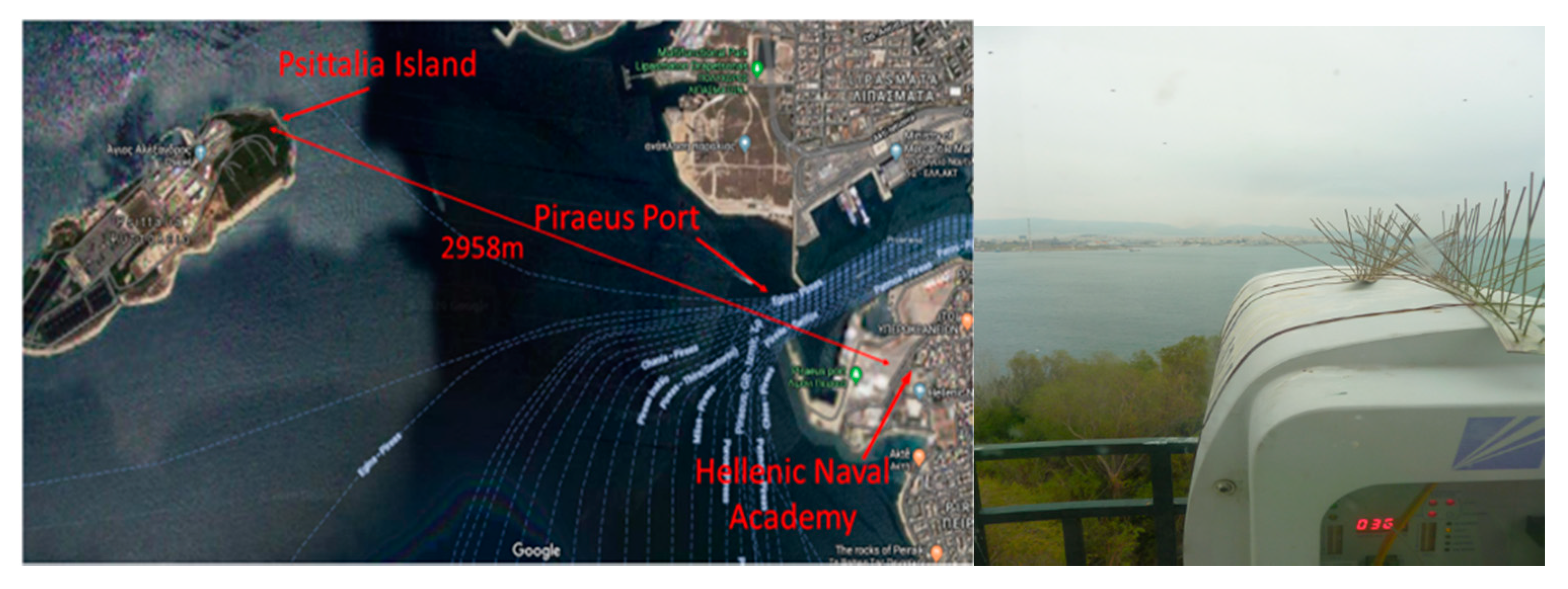
2. Data Acquisition
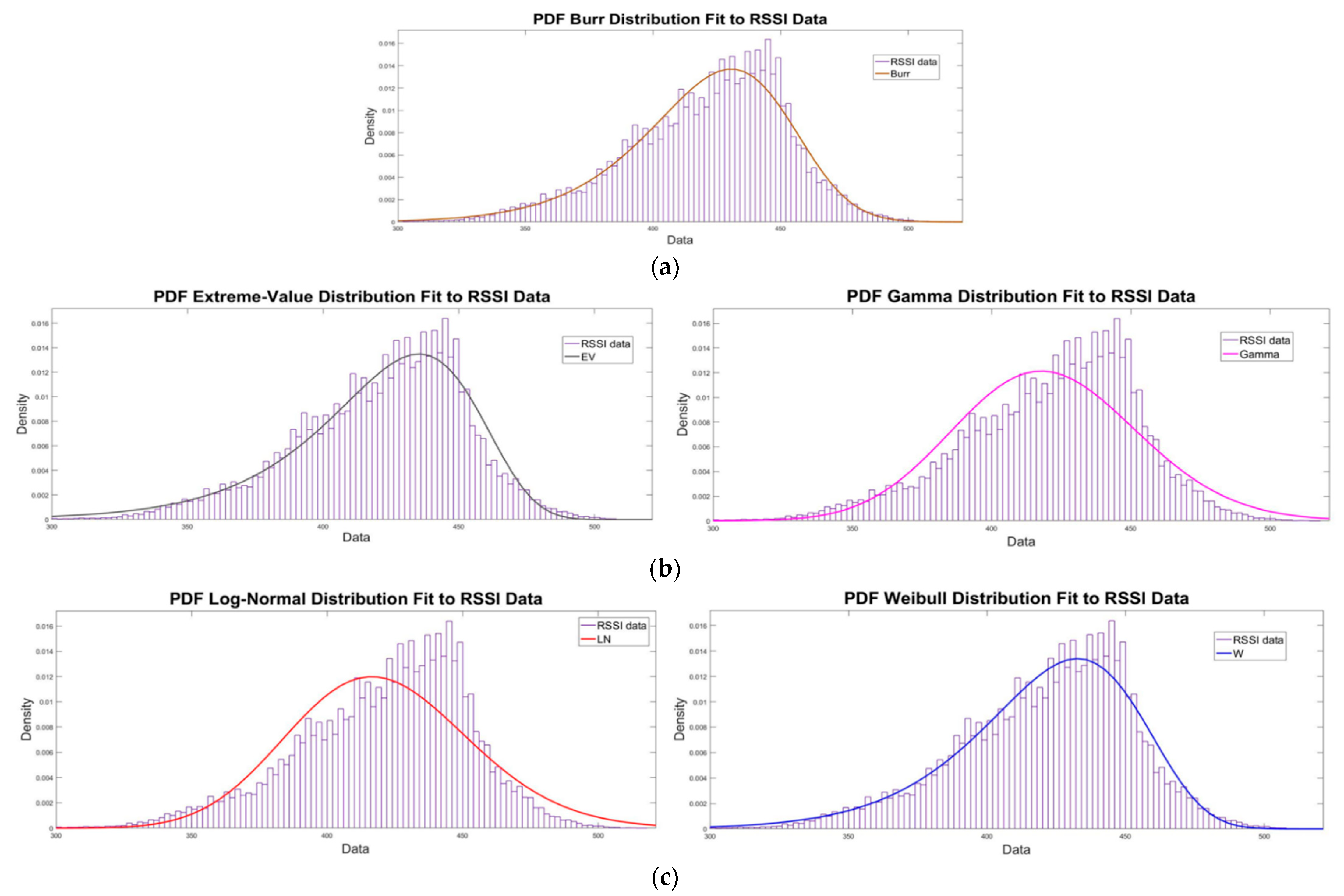
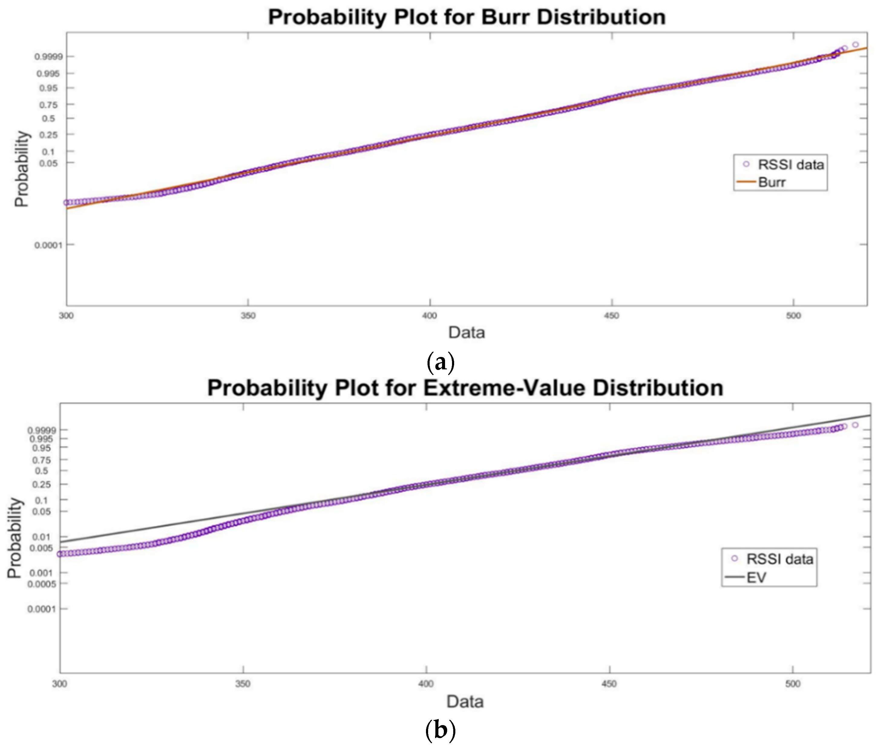
3. Results
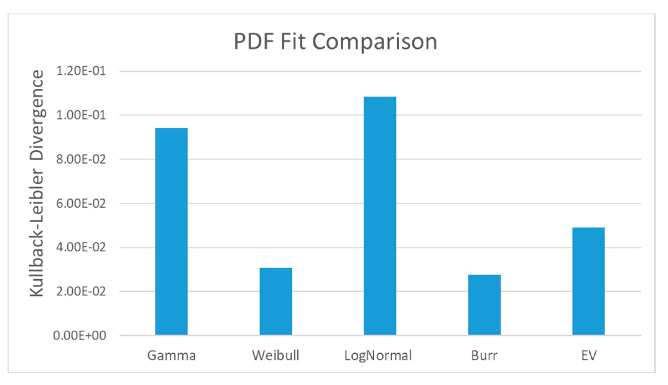
3.1. Kullback–Leibler Divergence
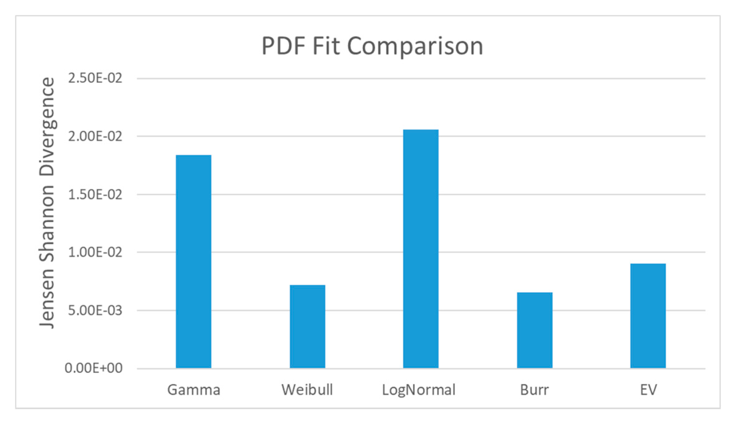
3.2. Jensen–Shannon Divergence
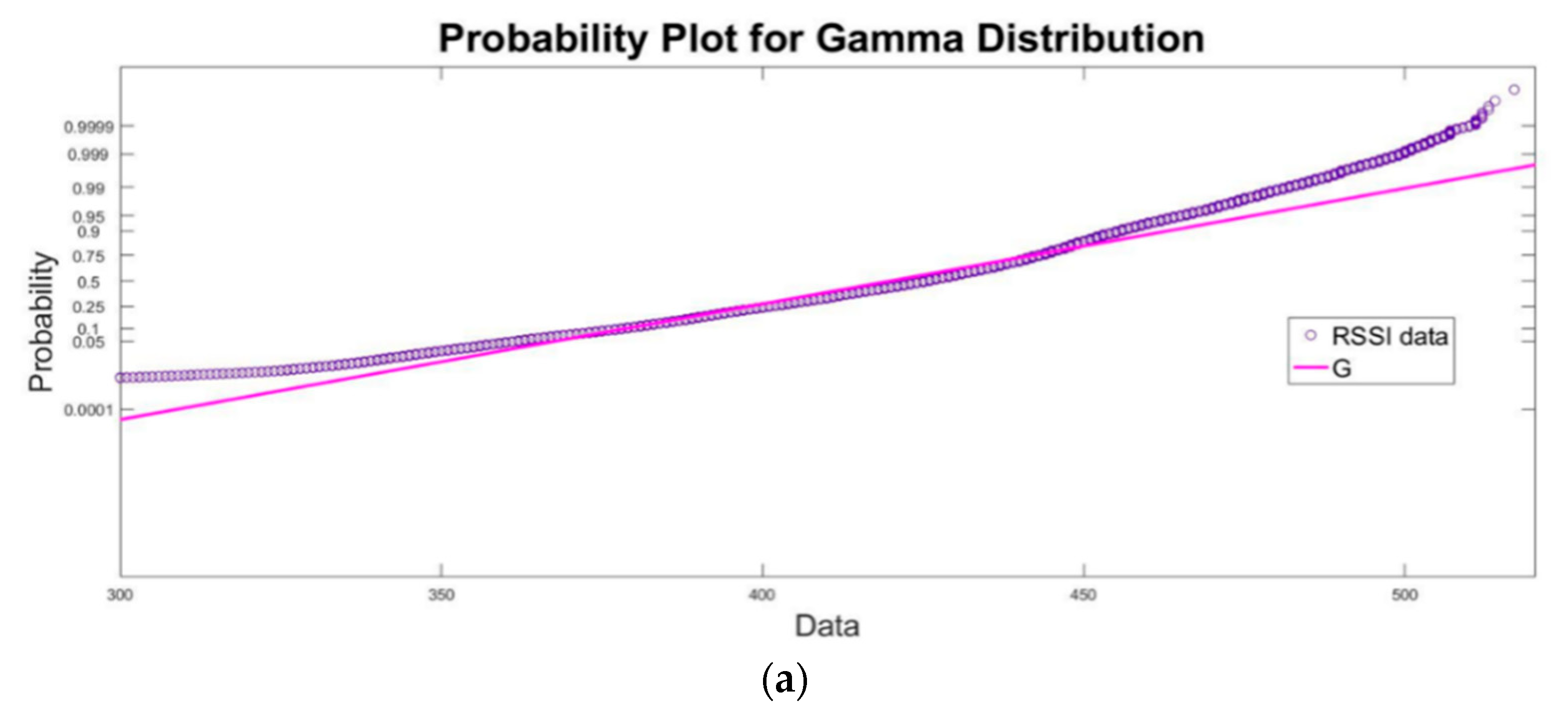
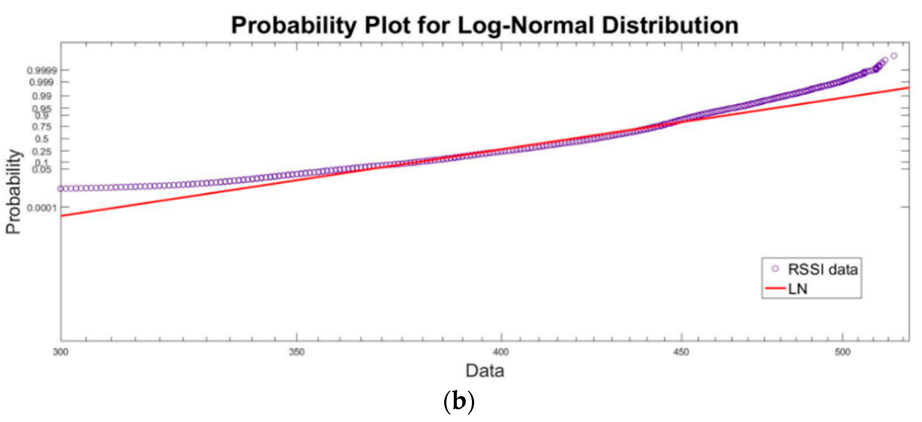
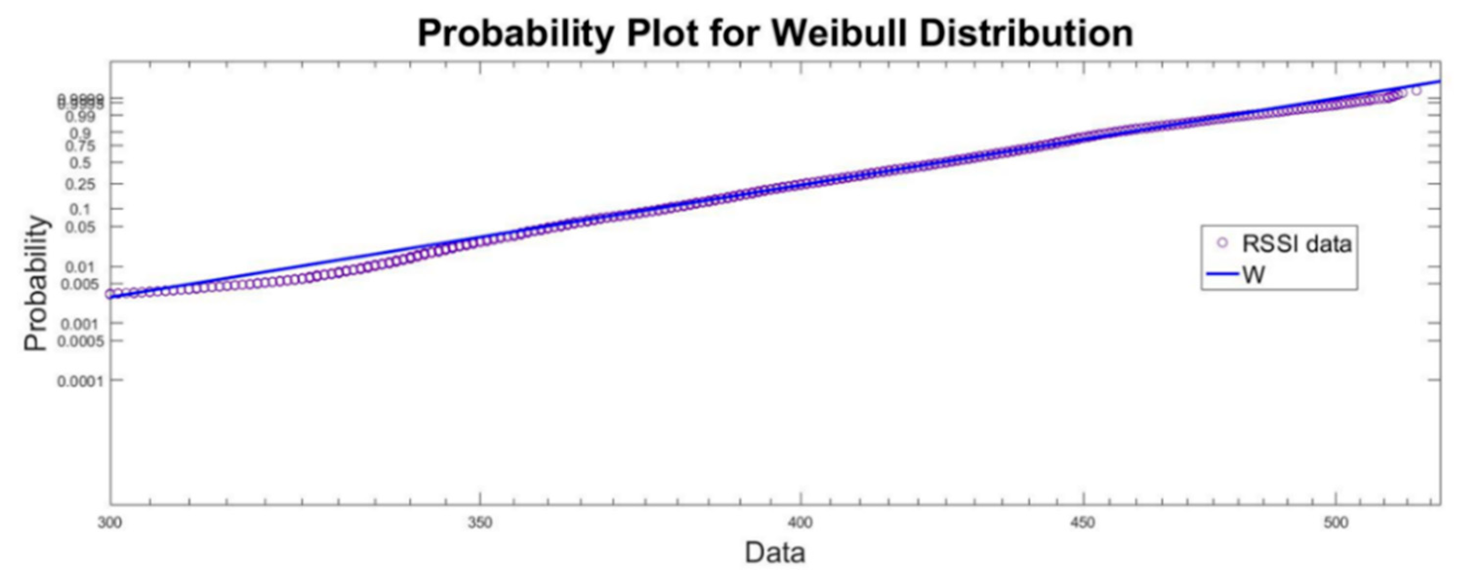
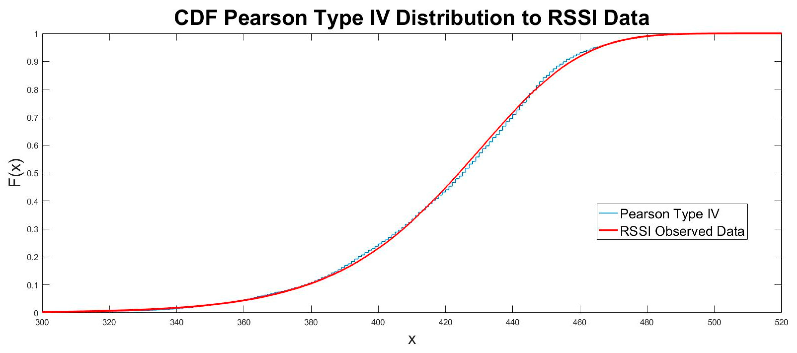
3.3. Pearson Distribution Family
4. Conclusions
Author Contributions
Funding
Institutional Review Board Statement
Informed Consent Statement
Conflicts of Interest
References
- Barrios, R.; Dios, F. Wireless Optical Communications through the Turbulent Atmosphere: A Review; Optical Communications Systems; Das, N., Ed.; InTech: Rijeka, Croatia, 2012; ISBN 978-953-51-0170-3. [Google Scholar]
- Jurado-Navas, A.; Garrido-Balsells, J.-M.; Paris, J.F.; Puerta-Notario, A. A Unifying Statistical Model for Atmospheric Optical Scintillation. In Numerical Simulations of Physical and Engineering Processes; Awrejcewicz, J., Ed.; InTech: Rijeka, Croatia, 2011; ISBN 978-953-307-620-1. [Google Scholar]
- Peppas, K.P.; Alexandropoulos, G.C.; Xenos, E.D.; Maras, A. The Fischer-Snedecor F-Distribution Model for Turbulence-Induced Fading in Free-Space Optical Systems. J. Lightwave Technol. 2019, 38, 1286–1295. [Google Scholar] [CrossRef]
- Nistazakis, H.E.; Katsis, A.; Tombras, G.S. On the Reliability and Performance of FSO and Hybrid FSO Communication Systems over Turbulent Channels; Nova Science Publishers, Inc.: Hauppauge, NY, USA, 2010; ISBN 978-1-61761-735-5. [Google Scholar]
- Garrido-Balsells, J.M.; Lopez-Martinez, F.J.; Castillo-Vázquez, M.; Jurado-Navas, A.; Puerta-Notario, A. Performance analysis of FSO communications under LOS blockage. Opt. Express 2017, 25, 25278–25294. [Google Scholar] [CrossRef] [PubMed] [Green Version]
- Varotsos, G.K.; Stassinakis, A.N.; Nistazakis, H.E.; Tsigopoulos, A.D.; Peppas, K.P.; Aidinis, C.J.; Tombras, G.S. Probability of fade estimation for FSO links with time dispersion and turbulence modeled with the gamma–gamma or the I-K distribution. Optik 2014, 125, 7191–7197. [Google Scholar] [CrossRef]
- Peppas, K.; Stassinakis, A.; Nistazakis, H.; Tombras, G. Capacity Analysis of Dual Amplify-and-Forward Relayed Free-Space Optical Communication Systems Over Turbulence Channels with Pointing Errors. J. Opt. Commun. Netw. 2013, 5, 1032–1042. [Google Scholar] [CrossRef]
- Wayne, D. The Pdf of Irradiance for A Free-Space Optical Communications Channel: A Physics Based Model. Ph.D. Thesis, University of Central Florida, Orlando, FL, USA, 2010. [Google Scholar]
- Nistazakis, H.E.; Karagianni, E.A.; Tsigopoulos, A.D.; Fafalios, M.E.; Tombras, G.S. Average Capacity of Optical Wireless Communication Systems Over Atmospheric Turbulence Channels. J. Lightwave Technol. 2009, 27, 974–979. [Google Scholar] [CrossRef]
- Korotkova, O.; Avramov-Zamurovic, S.; Malek-Madani, R.; Nelson, C. Probability density function of the intensity of a laser beam propagating in the maritime environment. Opt. Express 2011, 19, 20322–20331. [Google Scholar] [CrossRef] [PubMed] [Green Version]
- Ricardo, B. Exponentiated Weibull Fading Channel Model in Free-Space Optical Communications under Atmospheric Turbulence. Ph.D. Thesis, Polytechnic University of Catalonia, Barcelona, Spain, 2013. [Google Scholar]
- Kaushal, H.; Jain, V.K.; Kar, S. Free-Space Optical Channel Models; Springer: New Delhi, India, 2017. [Google Scholar] [CrossRef]
- Andrews, L.C.; Phillips, R.L.; Hopen, C.Y. Laser Beam Scintillation with Applications, 2nd ed.; SPIE: Bellingham, WA, USA, 2001. [Google Scholar]
- Majumdar, A.K. Free-space laser communication performance in the atmospheric channel. J. Opt. Fiber Commun. Rep. 2005, 2, 345–396. [Google Scholar] [CrossRef]
- Lionis, A.; Peppas, K.; Nistazakis, H.E.; Tsigopoulos, A.D.; Cohn, K. Experimental Performance Analysis of an Optical Communication Channel over Maritime Environment. Electronics 2020, 9, 1109. [Google Scholar] [CrossRef]
- Haluška, R.; Šuľaj, P.; Ovseník, Ľ.; Marchevský, S.; Papaj, J.; Doboš, Ľ. Prediction of Received Optical Power for Switching Hybrid FSO/RF System. Electronics 2020, 9, 1261. [Google Scholar] [CrossRef]
- Latal, J.; Vitasek, J.; Hajek, L.; Vanderka, A.; Koudelka, P.; Kepak, S.; Vasinek, V. Regression Models Utilization for RSSI Prediction of Professional FSO Link with Regards to Atmosphere Phenomena. In Proceedings of the 2016 International Conference on Broadband Communications for Next Generation Networks and Multimedia Applications (CoBCom), Graz, Austria, 14–16 September 2016. [Google Scholar]
- Hajek, L.; Vitasek, J.; Vanderka, A.; Latal, J.; Perecar, F.; Vasinek, V. Statistical prediction of the atmospheric behavior for free space optical link. In Proceedings of the SPIE 9614, Laser Communication and Propagation through the Atmosphere and Oceans IV, San Diego, CA, USA, 4 September 2015. [Google Scholar]
- Tóth, J.; Ovseník, L.; Turán, J.; Michaeli, L.; Márton, M. Classification prediction analysisof RSSI parameter in hard switching process for FSO/RF systems. Measurement 2017, 116, 602–610. [Google Scholar] [CrossRef]
- Lionis, A.; Peppas, K.; Nistazakis, H.E.; Tsigopoulos, A.D.; Cohn, K. Statistical modeling of received signal strength for an FSO link over maritime environment. Opt. Commun. 2021, 489, 126858. [Google Scholar] [CrossRef]
- Kullback, S.; Leibler, R. On Information and Sufficiency. Ann. Math. Stat. 1951, 22, 79–86. [Google Scholar] [CrossRef]
- Cover, T.M.; Thomas, J.A. Elements of Information Theory; John Wiley & Sons: Hoboken, NJ, USA, 2012. [Google Scholar]
- Fuglede, B.; Topsoe, F. Jensen-Shannon divergence and Hilbert space embedding. In Proceedings of the International Symposium on Information Theory, Chicago, IL, USA, 27 June–2 July 2004; p. 30, ISBN 978-0-7803-8280-0. [Google Scholar] [CrossRef]
- Nielsen, F. On a Generalization of the Jensen-Shannon Divergence and the Jensen-Shannon Centroid. Entropy 2020, 22, 221. [Google Scholar] [CrossRef] [Green Version]
- Nielsen, F. On the Jensen–Shannon Symmetrization of Distances Relying on Abstract Means. Entropy 2019, 21, 485. [Google Scholar] [CrossRef] [Green Version]
- Lahcene, B. On Pearson families of distributions and its applications. Afr. J. Math. Comput. Sci. Res. 2013, 6, 108–117. [Google Scholar] [CrossRef]
- Wei-Liem, L. On the characteristic function of Pearson type IV distributions. IMS Lect. Notes Monogr. Ser. 2004, 45, 171–179. [Google Scholar]


| Statistic | Value |
|---|---|
| Mean | 420.385927 |
| Standard Error | 0.084275342 |
| Median | 425 |
| Mode | 445 |
| Standard Deviation | 32.06917633 |
| Kurtosis | 1.481024233 |
| Skewness | −0.798160493 |
| Maximum | 187 |
| Minimum | 517 |
Publisher’s Note: MDPI stays neutral with regard to jurisdictional claims in published maps and institutional affiliations. |
© 2021 by the authors. Licensee MDPI, Basel, Switzerland. This article is an open access article distributed under the terms and conditions of the Creative Commons Attribution (CC BY) license (https://creativecommons.org/licenses/by/4.0/).
Share and Cite
Lionis, A.; Peppas, K.P.; Nistazakis, H.E.; Tsigopoulos, A. RSSI Probability Density Functions Comparison Using Jensen-Shannon Divergence and Pearson Distribution. Technologies 2021, 9, 26. https://0-doi-org.brum.beds.ac.uk/10.3390/technologies9020026
Lionis A, Peppas KP, Nistazakis HE, Tsigopoulos A. RSSI Probability Density Functions Comparison Using Jensen-Shannon Divergence and Pearson Distribution. Technologies. 2021; 9(2):26. https://0-doi-org.brum.beds.ac.uk/10.3390/technologies9020026
Chicago/Turabian StyleLionis, Antonios, Konstantinos P. Peppas, Hector E. Nistazakis, and Andreas Tsigopoulos. 2021. "RSSI Probability Density Functions Comparison Using Jensen-Shannon Divergence and Pearson Distribution" Technologies 9, no. 2: 26. https://0-doi-org.brum.beds.ac.uk/10.3390/technologies9020026