
Evaluation of Thoracic Equivalent Multiport Circuits Using an Electrical Impedance Tomography Hardware Simulation Interface

 ,
, 
Abstract
:1. Introduction
2. EIT Principle
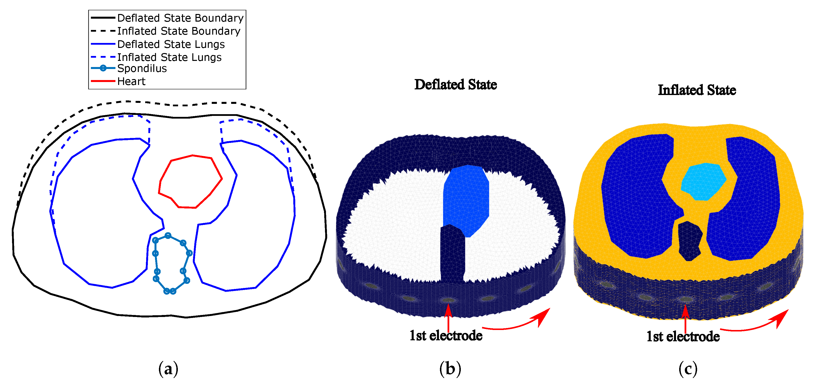
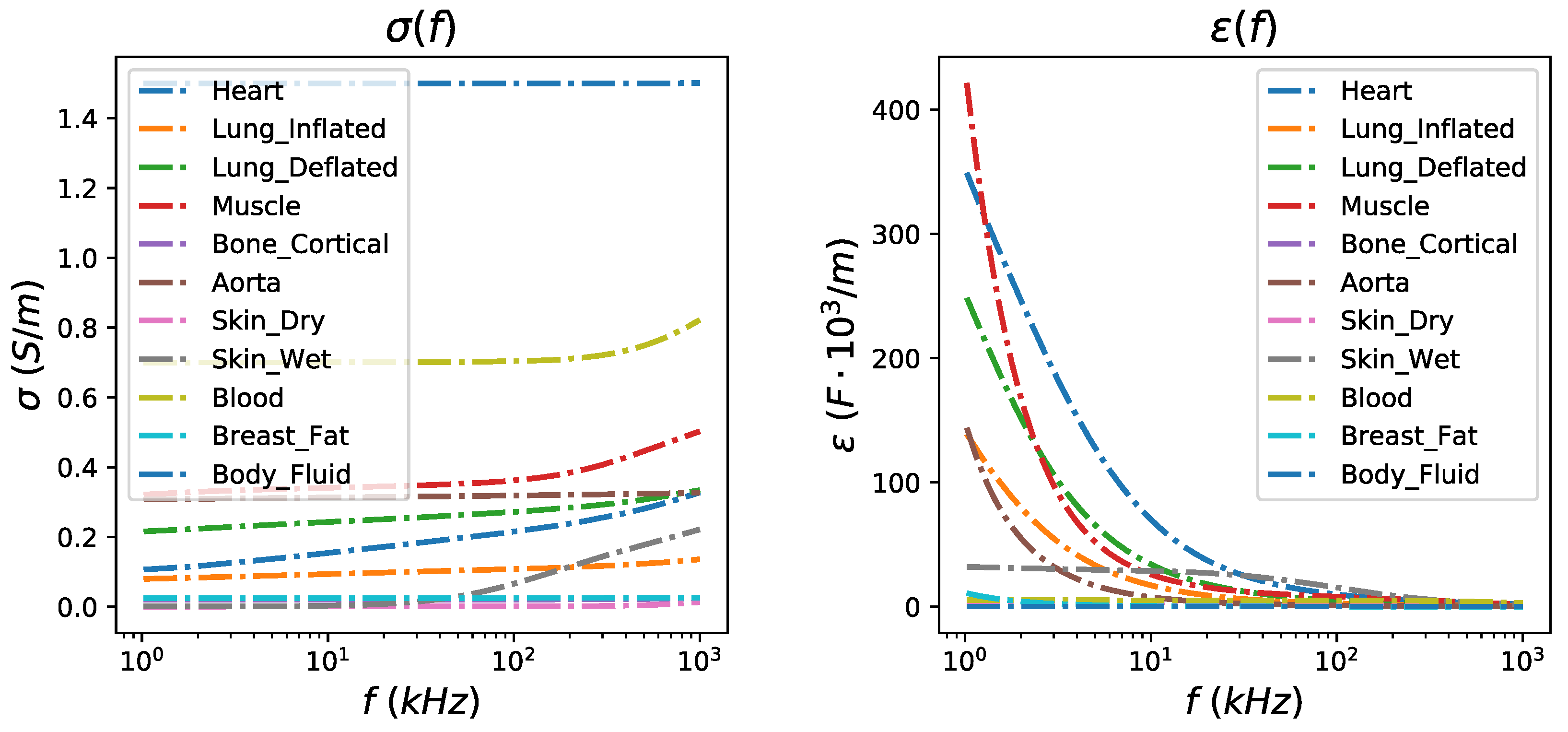
3. Thoracic Structures
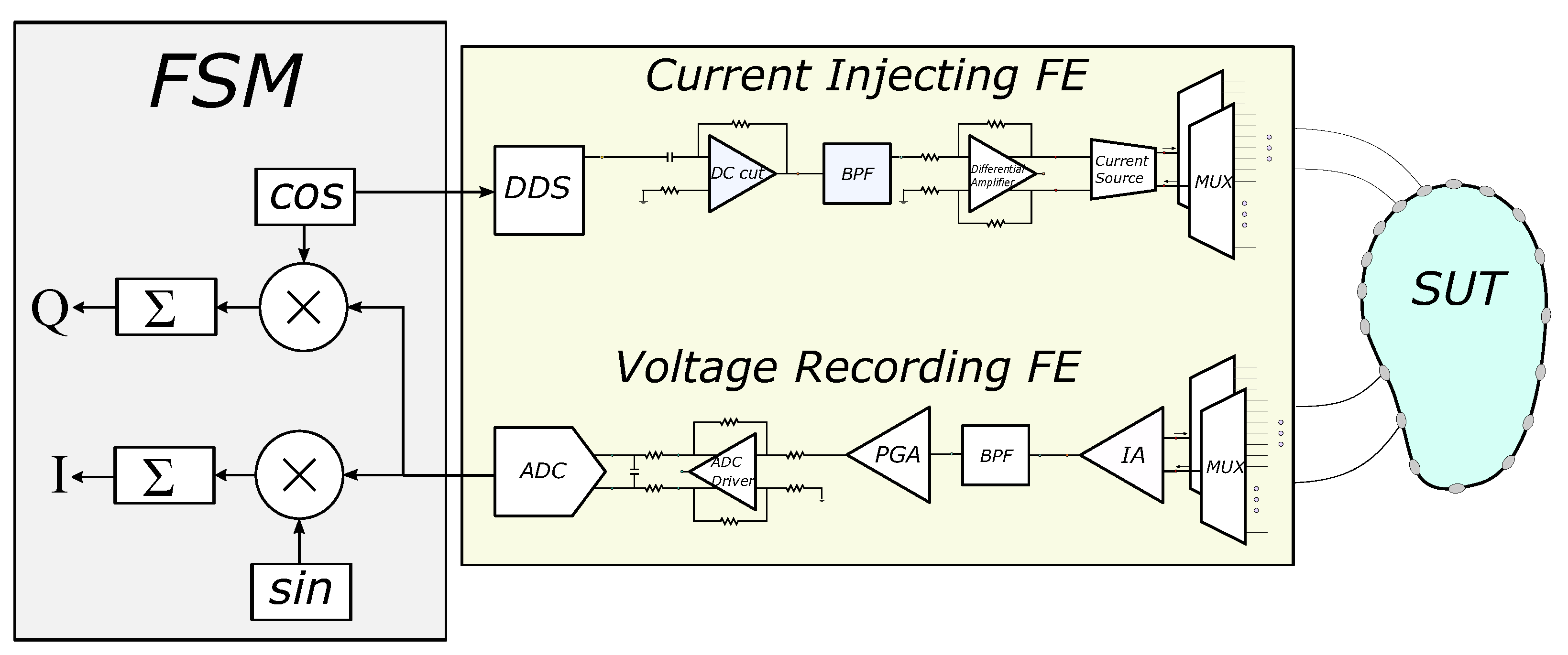
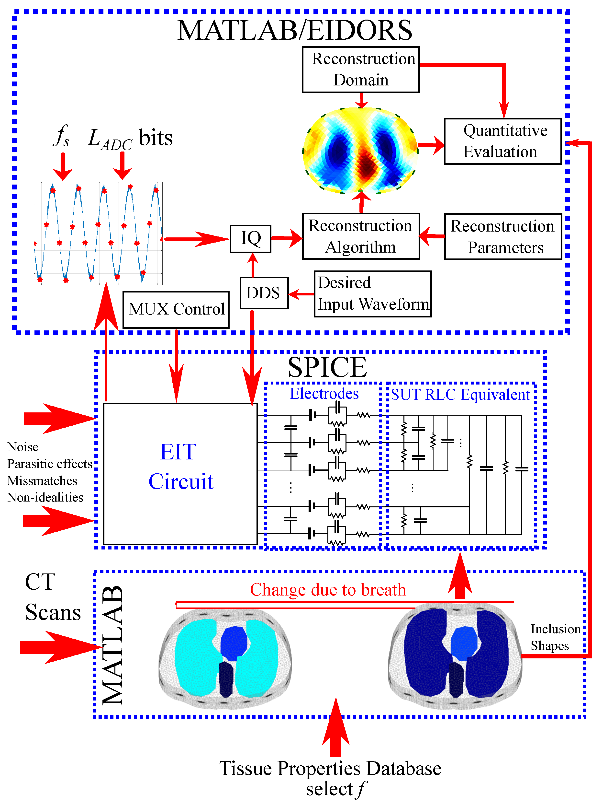
4. Simulation Interface
4.1. F.E.M. to RLC Equivalent Circuit Transformation
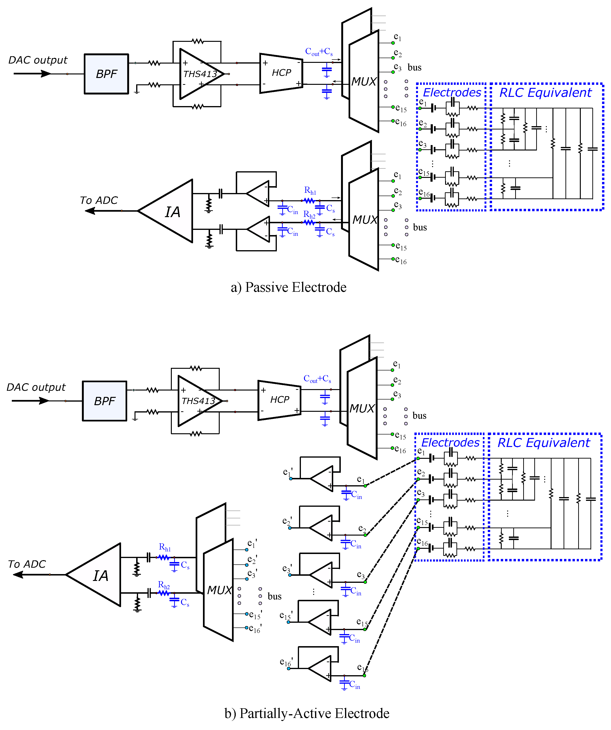
4.2. EIT SPICE Circuitry
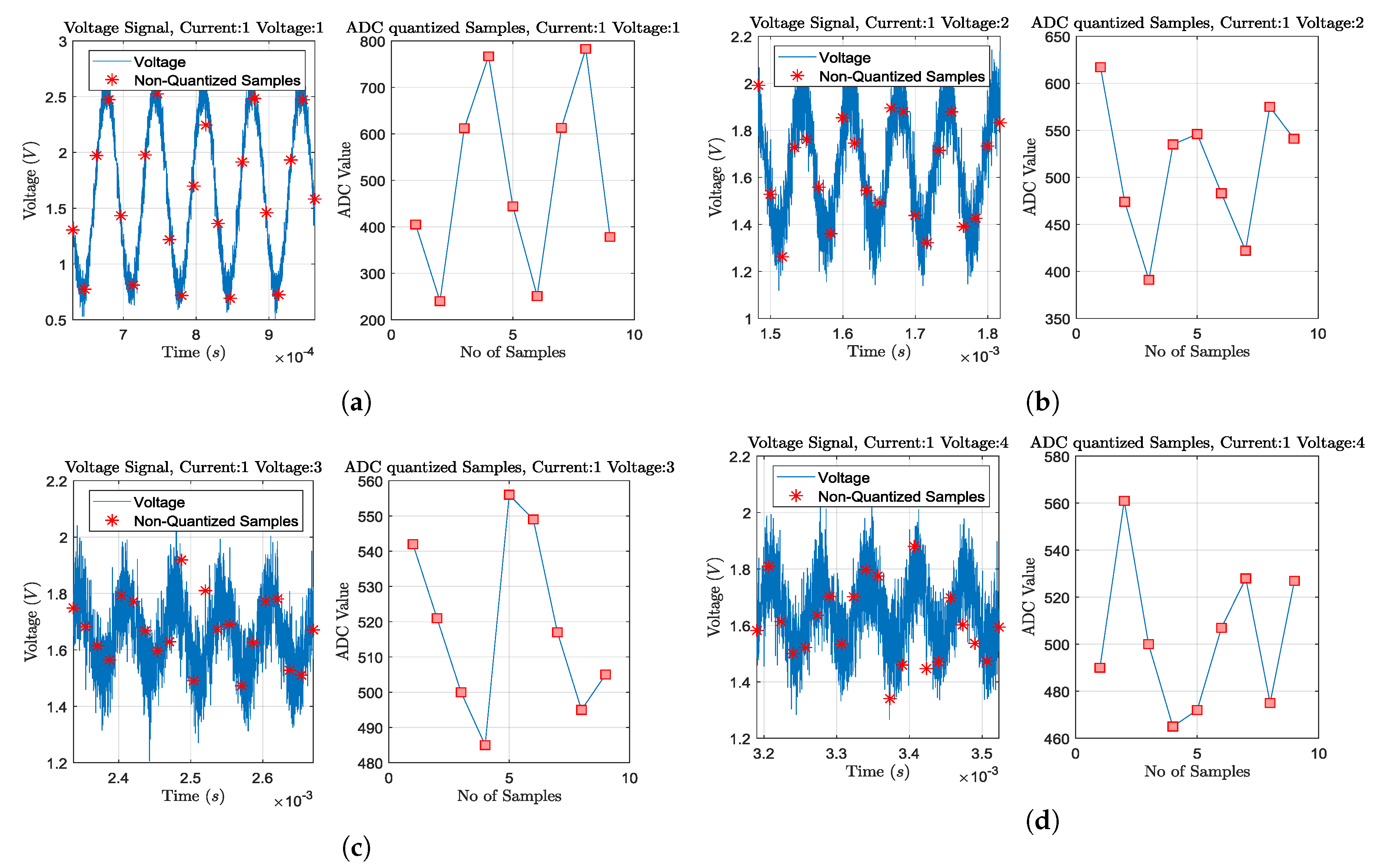
4.3. Sampling and Digital Signal Processing
5. Reconstruction and Evaluation Method
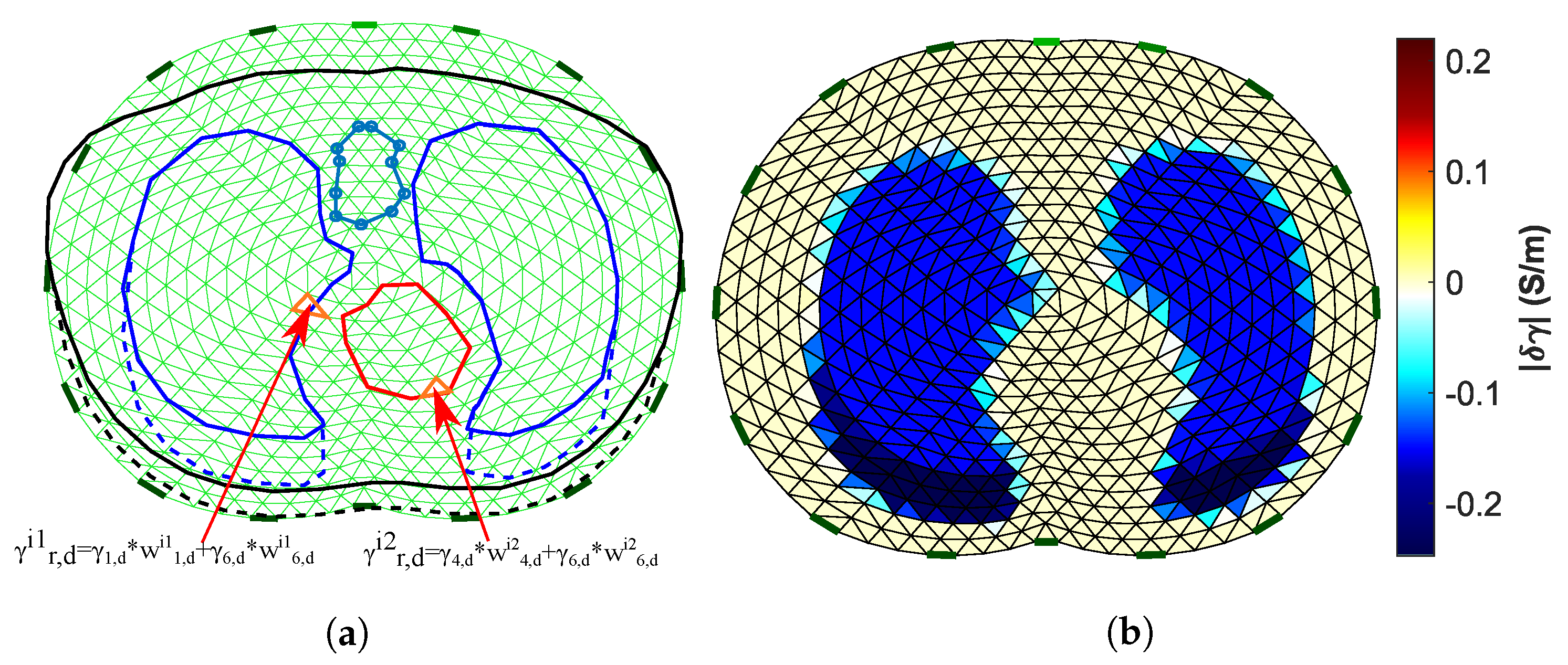
5.1. Image Reconstruction
5.2. Image Evaluation Method
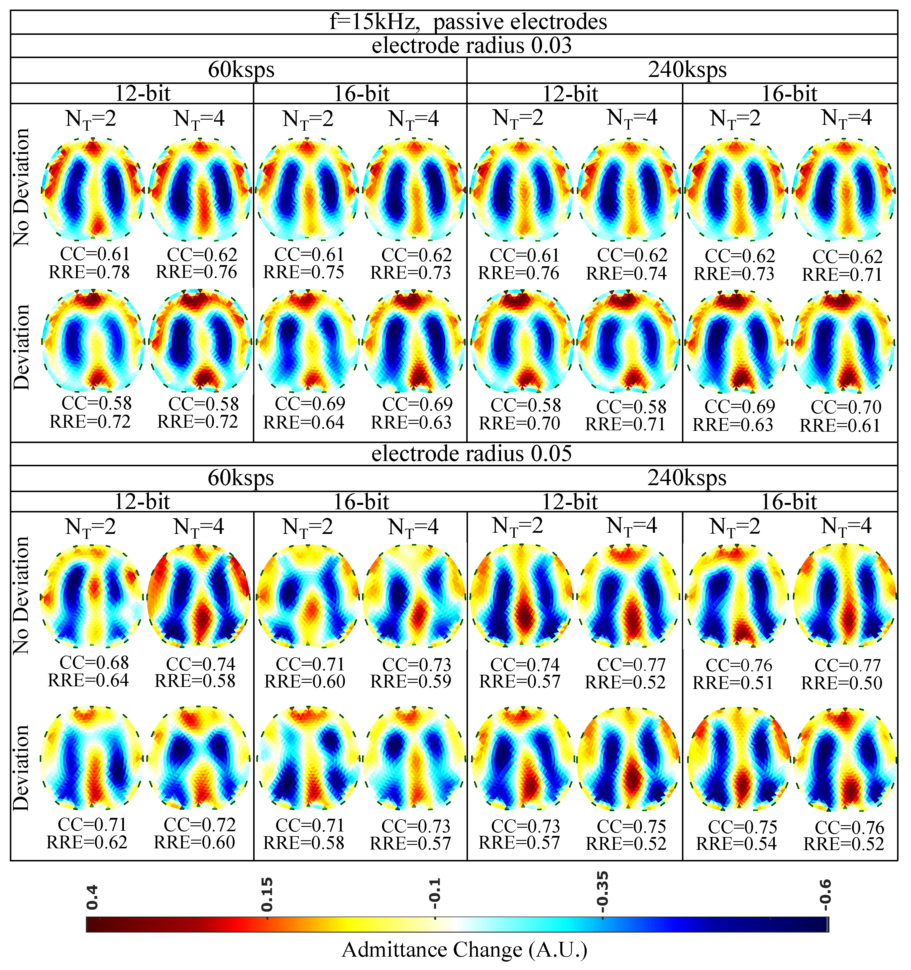
6. Results and Discussion
6.1. Simulation Cases
6.2. Simulation Results
6.3. Discussion
7. Conclusions
Author Contributions
Funding
Conflicts of Interest
References
- Holder, D.S. (Ed.) Electrical Impedance Tomography: Methods, History and Applications; CRC Press: Boca Raton, FL, USA, 2004. [Google Scholar]
- Bodenstein, M.; David, M.; Markstaller, K. Principles of electrical impedance tomography and its clinical application. Crit. Care Med. 2009, 37, 713–724. [Google Scholar] [CrossRef] [PubMed]
- Adler, A.; Boyle, A. Electrical Impedance Tomography: Tissue properties to image measures. IEEE Trans. Biomed. Eng. 2017, 64, 2494–2504. [Google Scholar] [PubMed]
- Wu, Y.; Jiang, D.; Bardill, A.; Bayford, R.; Demosthenous, A. A 122 fps, 1 MHz bandwidth multi-frequency wearable EIT belt featuring novel active electrode architecture for neonatal thorax vital sign monitoring. IEEE Trans. Biomed. Circuits Syst. 2019, 13, 927–937. [Google Scholar] [CrossRef] [Green Version]
- Wu, Y.; Hanzaee, F.F.; Jiang, D.; Bayford, R.H.; Demosthenous, A. Electrical Impedance Tomography for Biomedical Applications: Circuits and Systems Review. IEEE Open J. Circuits Syst. 2021, 2, 380–397. [Google Scholar] [CrossRef]
- Lionheart, W.R. EIT reconstruction algorithms: Pitfalls, challenges and recent developments. Physiol. Meas. 2004, 25, 125. [Google Scholar] [CrossRef] [PubMed] [Green Version]
- Shi, X.; Li, W.; You, F.; Huo, X.; Xu, C.; Ji, Z.; Dong, X. High-precision electrical impedance tomography data acquisition system for brain imaging. IEEE Sens. J. 2018, 18, 5974–5984. [Google Scholar] [CrossRef]
- Nguyen, D.T.; Jin, C.; Thiagalingam, A.; McEwan, A.L. A review on electrical impedance tomography for pulmonary perfusion imaging. Physiol. Meas. 2012, 33, 695. [Google Scholar] [CrossRef]
- Rao, A.; Teng, Y.C.; Schaef, C.; Murphy, E.K.; Arshad, S.; Halter, R.J.; Odame, K. An analog front end ASIC for cardiac electrical impedance tomography. IEEE Trans. Biomed. Circuits Syst. 2018, 12, 729–738. [Google Scholar] [CrossRef]
- Grychtol, B.; Lionheart, W.R.; Bodenstein, M.; Wolf, G.K.; Adler, A. Impact of model shape mismatch on reconstruction quality in electrical impedance tomography. IEEE Trans. Med. Imaging 2012, 31, 1754–1760. [Google Scholar] [CrossRef] [Green Version]
- Biguri, A.; Grychtol, B.; Adler, A.; Soleimani, M. Tracking boundary movement and exterior shape modelling in lung EIT imaging. Physiol. Meas. 2015, 36, 1119. [Google Scholar] [CrossRef]
- Wilson, A.J.; Milnes, P.; Waterworth, A.R.; Smallwood, R.H.; Brown, B.H. Mk3.5: A modular, multi-frequency successor to the Mk3a EIS/EIT system. Physiol. Meas. 2000, 22, 49–54. [Google Scholar] [CrossRef]
- Cook, R.D.; Saulnier, G.J.; Gisser, D.G.; Goble, J.C.; Newell, J.C.; Isaacson, D. ACT3: A high-speed, high-precision electrical impedance tomograph. IEEE Trans. Biomed. Eng. 1994, 41, 713–722. [Google Scholar] [CrossRef] [Green Version]
- Liu, N.; Saulnier, G.J.; Newell, J.C.; Isaacson, D.; Kao, T.-J. ACT4: A high-precision, multi-frequency electrical impedance tomograph. In Proceedings of the 6th Conference on Biomedical Applications of Electrical Impedance Tomography, London, UK, 22–24 June 2005. [Google Scholar]
- Wi, H.; Sohal, H.; McEwan, A.L.; Woo, E.J.; Oh, T.I. Multi-Frequency Electrical Impedance Tomography System With Automatic Self-Calibration for Long-Term Monitoring. IEEE Trans. Biomed. Circuits Syst. 2013, 8, 119–128. [Google Scholar]
- Mellenthin, M.M.; Mueller, J.L.; De Camargo, E.D.L.B.; De Moura, F.S.; Santos, T.B.R.; Lima, R.G.; Alsaker, M. The ACE1 electrical impedance tomography system for thoracic imaging. IEEE Trans. Instrum. Meas. 2018, 68, 3137–3150. [Google Scholar] [CrossRef]
- Wu, Y.; Jiang, D.; Bardill, A.; De Gelidi, S.; Bayford, R.; Demosthenous, A. A high frame rate wearable EIT system using active electrode ASICs for lung respiration and heart rate monitoring. IEEE Trans. Circuits Syst. I Regul. Pap. 2018, 65, 3810–3820. [Google Scholar] [CrossRef]
- Gaggero, P.O.; Adler, A.; Brunner, J.; Seitz, P. Electrical impedance tomography system based on active electrodes. Physiol. Meas. 2012, 33, 831. [Google Scholar] [CrossRef] [PubMed] [Green Version]
- Guermandi, M.; Cardu, R.; Scarselli, E.F.; Guerrieri, R. Active electrode IC for EEG and electrical impedance tomography with continuous monitoring of contact impedance. IEEE Trans. Biomed. Circuits Syst. 2014, 9, 21–33. [Google Scholar] [CrossRef]
- XMurphy, E.K.; Takhti, M.; Skinner, J.; Halter, R.J.; Odame, K. Signal-to-noise ratio analysis of a phase-sensitive voltmeter for electrical impedance tomography. IEEE Trans. Biomed. Circuits Syst. 2016, 11, 360–369. [Google Scholar] [CrossRef]
- Takhti, M.; Odame, K. Structured design methodology to achieve a high SNR electrical impedance tomography. IEEE Trans. Biomed. Circuits Syst. 2019, 13, 364–375. [Google Scholar] [CrossRef]
- Takhti, M.; Odame, K. A power adaptive, 1.22-pW/Hz, 10-MHz read-out front-end for bio-impedance measurement. IEEE Trans. Biomed. Circuits Syst. 2019, 13, 725–734. [Google Scholar] [CrossRef]
- Rao, A.; Murphy, E.K.; Halter, R.J.; Odame, K.M. A 1 MHz miniaturized electrical impedance tomography system for prostate imaging. IEEE Trans. Biomed. Circuits Syst. 2020, 14, 787–799. [Google Scholar] [CrossRef] [PubMed]
- Eberdt, M.; Brown, P.K.; Lazzi, G. Two-dimensional SPICE-linked multiresolution impedance method for low-frequency electromagnetic interactions. IEEE Trans. Biomed. Eng. 2003, 50, 881–889. [Google Scholar] [CrossRef]
- Boyle, A.; Adler, A. Integrating Circuit Simulation with EIT FEM Models. In Proceedings of the 19th Conference on Biomedical Applications of Electrical Impedance Tomography, Edinburgh, UK, 11–13 June 2018; p. 20. [Google Scholar]
- Adler, A.; Lionheart, W.R. Uses and abuses of EIDORS: An extensible software base for EIT. Physiol. Meas. 2006, 27, S25. [Google Scholar] [CrossRef] [Green Version]
- Dimas, C.; Uzunoglu, N.; Sotiriadis, P.P. Electrical impedance tomography image reconstruction: Impact of hardware noise and errors. In Proceedings of the 2019 8th International Conference on Modern Circuits and Systems Technologies (MOCAST), Thessaloniki, Greece, 13–15 May 2019; pp. 1–4. [Google Scholar]
- Dimas, C.; Uzunoglu, N.; Sotiriadis, P.P. A parametric EIT system spice simulation with phantom equivalent circuits. Technologies 2020, 8, 13. [Google Scholar] [CrossRef] [Green Version]
- Dimas, C.; Alimisis, V.; Sotiriadis, P.P. SPICE and MATLAB simulation and evaluation of Electrical Impedance Tomography readout chain using phantom equivalents. In Proceedings of the 2020 European Conference on Circuit Theory and Design (ECCTD), Sofia, Bulgaria, 7–10 September 2020; pp. 1–4. [Google Scholar]
- Adler, A.; Gaggero, P.O.; Maimaitijiang, Y. Adjacent stimulation and measurement patterns considered harmful. Physiol. Meas. 2011, 32, 731. [Google Scholar] [CrossRef] [PubMed]
- Tomicic, V.; Cornejo, R. Lung monitoring with electrical impedance tomography: Technical considerations and clinical applications. J. Thorac. Dis. 2019, 11, 3122. [Google Scholar] [CrossRef]
- Kolehmainen, V.; Vauhkonen, M.; Karjalainen, P.A.; Kaipio, J.P. Assessment of errors in static electrical impedance tomography with adjacent and trigonometric current patterns. Physiol. Meas. 1997, 18, 289. [Google Scholar] [CrossRef]
- Dimas, C.; Sotiriadis, P.P. Electrical impedance tomography image reconstruction for adjacent and opposite strategy using FEMM and EIDORS simulation models. In Proceedings of the 2018 7th International Conference on Modern Circuits and Systems Technologies (MOCAST), Thessaloniki, Greece, 7–9 May 2018; pp. 1–4. [Google Scholar]
- Silva, O.L.; Lima, R.G.; Martins, T.C.; De Moura, F.S.; Tavares, R.S.; Tsuzuki, M.S.G. Influence of current injection pattern and electric potential measurement strategies in electrical impedance tomography. Control Eng. Pract. 2017, 58, 276–286. [Google Scholar] [CrossRef]
- Simini, F.; Bertemes-Filho, P. Bioimpedance in Biomedical Applications and Research; Springer: New York, NY, USA, 2018. [Google Scholar]
- Avery, J.; Dowrick, T.; Witkowska-Wrobel, A.; Faulkner, M.; Aristovich, K.; David, H. Simultaneous EIT and EEG using frequency division multiplexing. Physiol. Meas. 2019, 40, 3. [Google Scholar] [CrossRef]
- Kassanos, P.; Constantinou, L.; Triantis, I.F.; Demosthenous, A. An integrated analog readout for multi-frequency bioimpedance measurements. IEEE Sens. J. 2018, 14, 2792–2800. [Google Scholar] [CrossRef]
- Hong, S.; Lee, J.; Bae, J.; Yoo, H.J. A 10.4 mW electrical impedance tomography SoC for portable real-time lung ventilation monitoring system. IEEE J. Solid-State Circuits 2015, 50, 2501–2512. [Google Scholar] [CrossRef]
- Schöberl, J. NETGEN An advancing front 2D/3D-mesh generator based on abstract rules. Comput. Vis. Sci. 1997, 1, 41–52. [Google Scholar] [CrossRef]
- Gabriel, S.; Gabriel, C.; Corthout, E. The dielectric properties of biological tissues: I. Literature survey. Phys. Med. Biol. 1996, 68, 2231. [Google Scholar] [CrossRef] [Green Version]
- Gabriel, S.; Lau, R.; Gabriel, C. The dielectric properties of biological tissues: II. Measurements in the frequency range 10 Hz to 20 GHz. Phys. Med. Biol. 1996, 41, 2251. [Google Scholar] [CrossRef] [PubMed] [Green Version]
- Gabriel, S.; Lau, R.; Gabriel, C. The dielectric properties of biological tissues: III. parametric models for the dielectric spectrum of tissues. Phys. Med. Biol. 1996, 41, 2271. [Google Scholar] [CrossRef] [PubMed] [Green Version]
- Liu, D.; Kolehmainen, V.; Siltanen, S.; Laukkanen, A.M.; Seppänen, A. Nonlinear difference imaging approach to three-dimensional electrical impedance tomography in the presence of geometric modeling errors. IEEE Trans. Biomed. Eng. 2015, 63, 1956–1965. [Google Scholar] [CrossRef]
- Hyvönen, N. Complete electrode model of electrical impedance tomography: Approximation properties and characterization of inclusions. SIAM J. Appl. Math. 2004, 64, 902–931. [Google Scholar] [CrossRef]
- Polydorides, N. Image Reconstrucion Algorithms for Soft-Field Tomography. Ph.D. Thesis, University of Manchester Institute of Science and Technology, Manchester, UK, 2002. [Google Scholar]
- Proenca, M. Resistor Networks and Finite Element Models. Ph.D. Thesis, University of Manchester, Manchester, UK, 2011. [Google Scholar]
- Franks, W.; Schenker, I.; Schmutz, P.; Hierlemann, A. Impedance Characterization and Modeling of Electrodes for Biomedical Applications. IEEE Trans. Biomed. Eng. 2005, 52, 7. [Google Scholar] [CrossRef]
- Da Silveira, D.V.; Button, N. Principles of Measurement and Transduction of Biomedical Variables; Academic Press (Elsevier): Cambridge, MA, USA, 2015. [Google Scholar]
- Albulbul, A. Evaluating Major Electrode Types for Idle Biological Signal Measurements for Modern Medical Technology. Bioengineering 2016, 3, 20. [Google Scholar] [CrossRef] [PubMed] [Green Version]
- Vauhkonen, M.; Vadasz, D.; Karjalainen, P.A.; Somersalo, E.; Kaipio, J.P. Tikhonov regularization and prior information in electrical impedance tomography. IEEE Trans. Med. Imaging 1998, 17, 285–293. [Google Scholar] [CrossRef]
- Hamilton, S.J.; Hauptmann, A. Deep D-bar: Real-time electrical impedance tomography imaging with deep neural networks. IEEE Trans. Med. Imaging 2020, 37, 2367–2377. [Google Scholar] [CrossRef] [Green Version]
- Liu, S.; Jia, J.; Zhang, Y.D.; Yang, Y. Image reconstruction in electrical impedance tomography based on structure-aware sparse Bayesian learning. IEEE Trans. Med. Imaging 2018, 37, 2090–2102. [Google Scholar] [CrossRef] [PubMed] [Green Version]
- Liu, S.; Cao, R.; Huang, Y.; Ouypornkochagorn, T.; Jia, J. Time sequence learning for electrical impedance tomography using Bayesian spatiotemporal priors. IEEE Trans. Instrum. Meas. 2020, 69, 6045–6057. [Google Scholar] [CrossRef] [Green Version]
- Cheng, K.S.; Isaacson, D.; Newell, J.C.; Gisser, D.G. Electrode models for electric current computed tomography. IEEE Trans. Biomed. Eng. 1989, 36, 918–924. [Google Scholar] [CrossRef] [PubMed] [Green Version]
- Somersalo, E.; Cheney, M.; Isaacson, D. Existence and uniqueness for electrode models for electric current computed tomography. SIAM J. Appl. Math. 1992, 52, 1023–1040. [Google Scholar] [CrossRef]
- Brown, B.H.; Seagar, A.D. The Sheffield data collection system. Clin. Phys. Physiol. Meas. 1987, 8, 91. [Google Scholar] [CrossRef]
- Adler, A.; Arnold, J.H.; Bayford, R.; Borsic, A.; Brown, B.; Dixon, P.; Faes, T.J.; Frerichs, I.; Gagnon, H.; Gärber, Y.; et al. GREIT: A unified approach to 2D linear EIT reconstruction of lung images. Physiol. Meas. 2009, 30, S35. [Google Scholar] [CrossRef] [PubMed]
- Martin, S.; Choi, C.T. A post-processing method for three-dimensional electrical impedance tomography. Sci. Rep. 2017, 7, 1–10. [Google Scholar] [CrossRef] [Green Version]
- Alimisis, V.; Dimas, C.; Pappas, G.; Sotiriadis, P.P. Analog Realization of Fractional-Order Skin-Electrode Model for Tetrapolar Bio-Impedance Measurements. Technologies 2020, 8, 61. [Google Scholar] [CrossRef]
- Yang, L.; Dai, M.; Xu, C.; Zhang, G.; Li, W.; Fu, F.; Shi, X.; Dong, X. The frequency spectral properties of electrode-skin contact impedance on human head and its frequency-dependent effects on frequency-difference EIT in stroke detection from 10 Hz to 1 MHz. PLoS ONE 2017, 12, e0170563. [Google Scholar] [CrossRef] [Green Version]
- Soleimani, M.; Gómez-Laberge, C.; Adler, A. Imaging of conductivity changes and electrode movement in EIT. Physiol. Meas. 2006, 27, S103. [Google Scholar] [CrossRef] [PubMed]


| Tissue | at 15 kHz (S/m) | at 15 kHz (F·Hz/m) | at 100 kHz (S/m) | at 100 kHz (F·Hz/m) |
|---|---|---|---|---|
| Heart | ||||
| Inflated Lung | ||||
| Deflated Lung | ||||
| Bones | ||||
| Skin and Fat | ||||
| Muscle and Plasma |
| Model | No of Elements () | No of Nodes () |
|---|---|---|
| Inflated, Uniform Electrodes, | 145,900 | 29,507 |
| Inflated, Uniform Electrodes, | 133,756 | 26,861 |
| Inflated, Non-Uniform Electrodes, | 146,000 | 29,542 |
| Inflated, Non-Uniform Electrodes, | 135,330 | 27,120 |
| Deflated, Uniform Electrodes, | 134,200 | 27,460 |
| Deflated, Uniform Electrodes, | 133,756 | 24,849 |
| Deflated, Non-Uniform Electrodes, | 133,529 | 27,328 |
| Deflated, Non-Uniform Electrodes, | 119,654 | 23,965 |
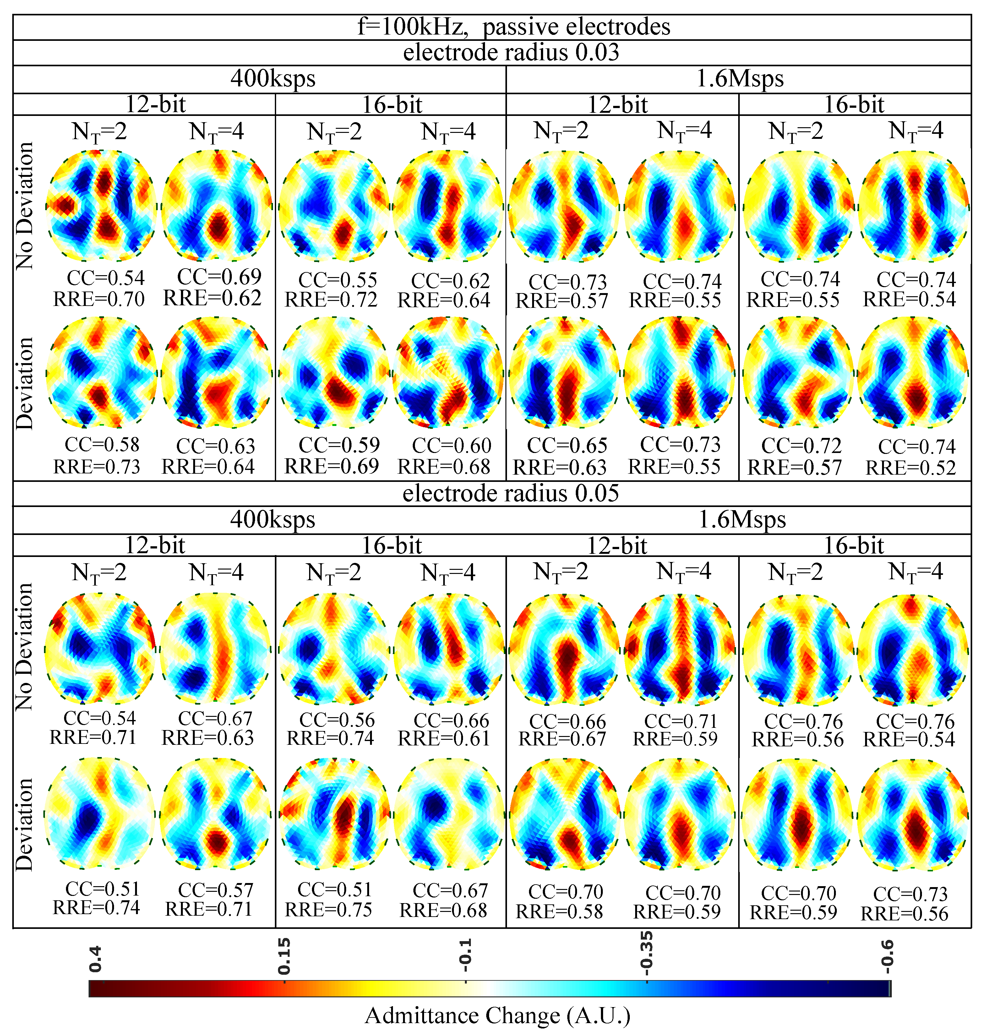
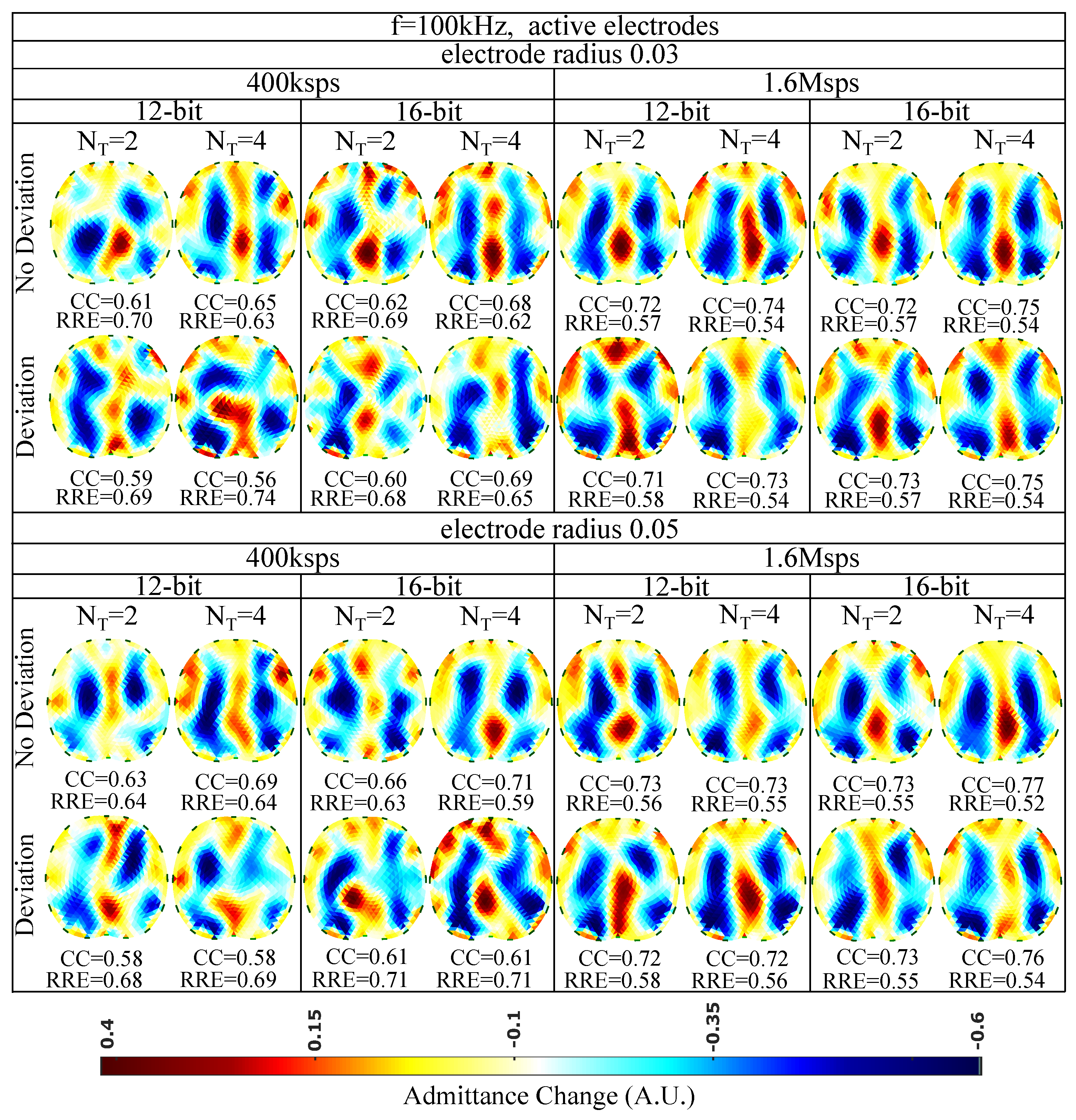
| f (kHz) | (bits) | (dB) | ||
|---|---|---|---|---|
| 15 | 12 | 2 | ||
| 15 | 12 | 4 | ||
| 15 | 12 | 2 | ||
| 15 | 12 | 4 | ||
| 15 | 16 | 2 | ||
| 15 | 16 | 4 | ||
| 15 | 16 | 2 | ||
| 15 | 16 | 4 | ||
| 100 | 12 | 2 | ||
| 100 | 12 | 4 | ||
| 100 | 12 | 2 | ||
| 100 | 12 | 4 | ||
| 100 | 16 | 2 | ||
| 100 | 16 | 4 | ||
| 100 | 16 | 2 | ||
| 100 | 16 | 4 |
Publisher’s Note: MDPI stays neutral with regard to jurisdictional claims in published maps and institutional affiliations. |
© 2021 by the authors. Licensee MDPI, Basel, Switzerland. This article is an open access article distributed under the terms and conditions of the Creative Commons Attribution (CC BY) license (https://creativecommons.org/licenses/by/4.0/).
Share and Cite
Dimas, C.; Alimisis, V.; Georgakopoulos, I.; Voudoukis, N.; Uzunoglu, N.; Sotiriadis, P.P. Evaluation of Thoracic Equivalent Multiport Circuits Using an Electrical Impedance Tomography Hardware Simulation Interface. Technologies 2021, 9, 58. https://0-doi-org.brum.beds.ac.uk/10.3390/technologies9030058
Dimas C, Alimisis V, Georgakopoulos I, Voudoukis N, Uzunoglu N, Sotiriadis PP. Evaluation of Thoracic Equivalent Multiport Circuits Using an Electrical Impedance Tomography Hardware Simulation Interface. Technologies. 2021; 9(3):58. https://0-doi-org.brum.beds.ac.uk/10.3390/technologies9030058
Chicago/Turabian StyleDimas, Christos, Vassilis Alimisis, Ioannis Georgakopoulos, Nikolaos Voudoukis, Nikolaos Uzunoglu, and Paul P. Sotiriadis. 2021. "Evaluation of Thoracic Equivalent Multiport Circuits Using an Electrical Impedance Tomography Hardware Simulation Interface" Technologies 9, no. 3: 58. https://0-doi-org.brum.beds.ac.uk/10.3390/technologies9030058