Article

Chaotic Jaya Approaches to Solving Electromagnetic Optimization Benchmark Problems

by
Leandro dos S. Coelho
1,2,
Viviana C. Mariani
1,3,
Sotirios K. Goudos
4,*,
Achilles D. Boursianis
4,
Konstantinos Kokkinidis
5 and
Nikolaos V. Kantartzis
6
1
Department of Electrical Engineering, Federal University of Parana, Curitiba 80210-170, Brazil
2
Industrial and Systems Engineering Graduate Program (PPGEPS), Pontifical Catholic University of Parana, Curitiba 80215-901, Brazil
3
Mechanical Engineering Graduate Program (PPGEM), Pontifical Catholic University of Parana, Curitiba 80215-901, Brazil
4
Department of Physics, Aristotle University of Thessaloniki, 54124 Thessaloniki, Greece
5
Department of Applied Informatics, University of Macedonia, 54636 Thessaloniki, Greece
6
Department of Electrical and Computer Engineering, Aristotle University of Thessaloniki, 54124 Thessaloniki, Greece
*
Author to whom correspondence should be addressed.
Submission received: 5 March 2021 / Revised: 20 April 2021 / Accepted: 12 May 2021 / Published: 2 June 2021

Abstract

:
The Jaya optimization algorithm is a simple, fast, robust, and powerful population-based stochastic metaheuristic that in recent years has been successfully applied in a variety of global optimization problems in various application fields. The essential idea of the Jaya algorithm is that the searching agents try to change their positions toward the best obtained solution by avoiding the worst solution at every generation. The important difference between Jaya and other metaheuristics is that Jaya does not require the tuning of its control, except for the maximum number of iterations and population size parameters. However, like other metaheuristics, Jaya still has the dilemma of an appropriate tradeoff between its exploration and exploitation abilities during the evolution process. To enhance the convergence performance of the standard Jaya algorithm in the continuous domain, chaotic Jaya (CJ) frameworks based on chaotic sequences are proposed in this paper. In order to obtain the performance of the standard Jaya and CJ approaches, tests related to electromagnetic optimization using two different benchmark problems are conducted. These are the Loney’s solenoid benchmark and a brushless direct current (DC) motor benchmark. Both problems are realized to evaluate the effectiveness and convergence rate. The simulation results and comparisons with the standard Jaya algorithm demonstrated that the performance of the CJ approaches based on Chebyshev-type chaotic mapping and logistic mapping can be competitive results in terms of both efficiency and solution quality in electromagnetics optimization.

1. Introduction

The Jaya algorithm, which was introduced by Rao [1], is a simple, flexible, and powerful population-based stochastic algorithm for handling problems with discontinuous and non-differentiable objective functions and has been successfully applied to different kinds of global optimization problems. The Jaya algorithm is an emerging metaheuristic based on the concept that the candidate solution obtained for a given global optimization problem should change its position toward the best solution by updating its values and avoiding the worst solution in the current population. The major advantage of the Jaya algorithm is that it does not require any control parameter settings. Thus, the algorithm may easily search to find the global or near-global solution of the optimization problem in the continuous domain. It only needs the essential population size and stopping condition (maximum number of iterations) for optimization. The other main characteristics of the Jaya algorithm are its simple structure in terms of formulation and fast convergence behavior.
Despite its simplicity and efficiency features, the standard Jaya algorithm suffers from some of the same shortcomings as other metaheuristic algorithms applied to global optimization. The Jaya algorithm can present premature convergence to a local optimum solution and has the possibility of being trapped into local optima solutions when dealing with complex multimodal optimization problems due to weak exploration ability and insufficient population diversity. In general, balancing between the exploration (diversification) and exploitation (intensification) capabilities is a challenging task in metaheuristics design during the global optimization process. To overcome these drawbacks, different variants to improve the performance of the standard Jaya optimizer have been proposed in the literature, such as self-adaptive Jaya [2], Jaya with Lévy flight [3], and shuffled Jaya [4].
To improve the global convergence ability of metaheuristics, chaotic sequences can be useful. Chaos is a nonlinear phenomenon characterized by a lack of periodicity, randomness, and ergodicity. Moreover, chaotic maps are sensitive to the initial conditions. Given the ergodicity and randomness of chaos, it can be an effective mechanism when employed for exploratory and exploitative purposes to avoid premature convergence for local optima during the searching process and enhance the convergence rate in metaheuristics in global optimization. From the recent literature [5,6,7,8], there are methods of integration of one-dimensional chaotic maps with optimizers.
The main contribution of our work is to introduce a modified version of Jaya using chaos sequences generated by chaotic maps (evolution function) that are discrete-time parametrized instead of uniformly distributed. Thus, by using the chaotic maps, we have been able to strengthen the original Jaya features and obtain robust and globally optimal solutions. The proposed chaotic Jaya (CJ) approaches combine exploitative local search and explorative global search processes efficiently by utilization of a chaotic map, introducing more diversity to produce candidate solutions. The proposed CJ approaches can lead to improving the acceleration capability toward the global solution in global optimization problems. Numerical results to the Loney’s solenoid benchmark problem [9,10] and a brushless direct current (DC) motor benchmark problem [11] are provided which demonstrate the usage and efficiency of the proposed CJ approaches.
The rest of the paper is organized into the following sections. Section 2 briefly describes the Loney’s solenoid, while Section 3 describes the brushless DC motor benchmark. After that, Section 4 covers the background information on the Jaya algorithm and the proposed CJ approaches. The performance of the Jaya approaches is evaluated on the optimization benchmarks and is compared to other metaheuristics in Section 5. Finally, we give the concluding remarks and the discussion for future works in Section 6.

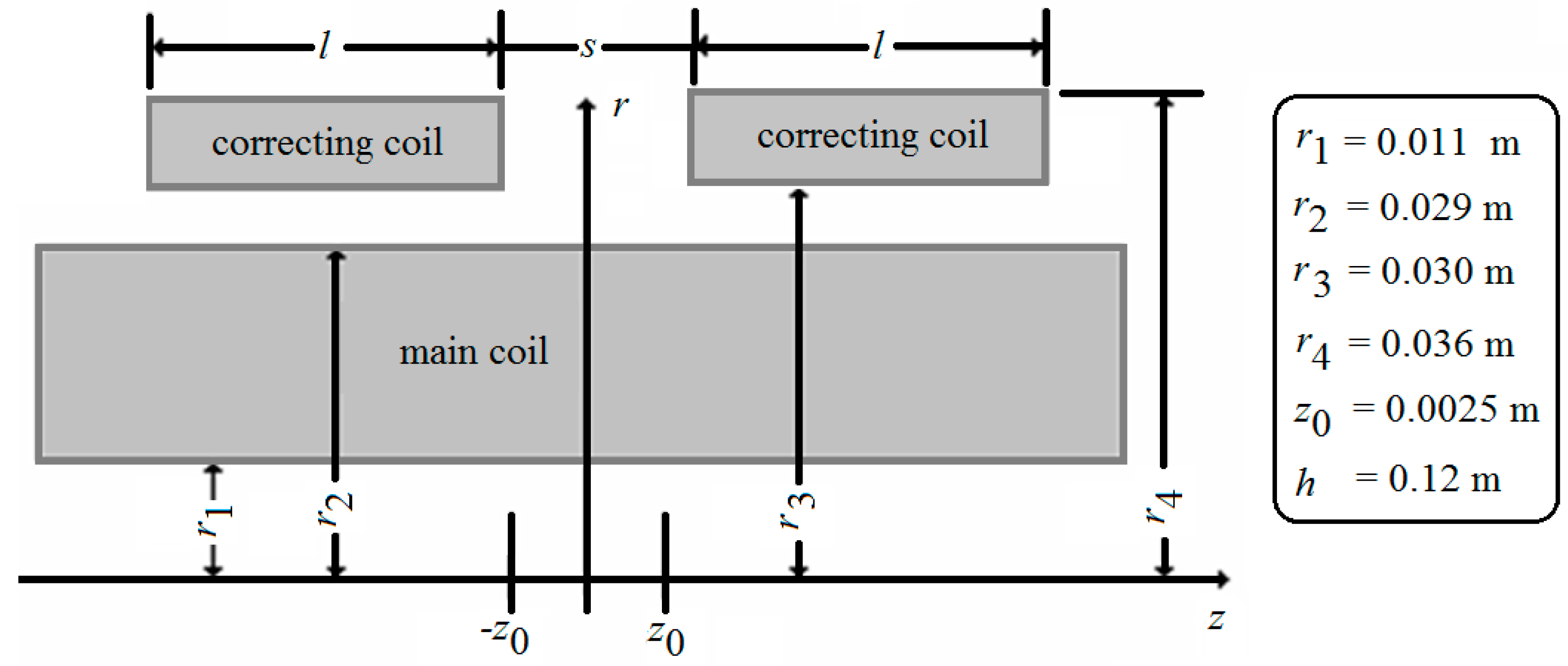
2. Loney’s Solenoid Design

The Loney’s solenoid belongs to the domain of nonlinear benchmark problems. It is considered a magnetostatic inverse problem. The solution of Loney’s solenoid design problem with local search methods that use derivatives can be resource intensive. Thus, the researchers, driven by this fact, are compelled to rely on metaheuristics for a solution. Metaheuristic algorithms are useful to handle different and complex global optimization problems, regardless of the nature of the problem itself.
The Loney’s solenoid benchmark problem is considered a testbed due to the rough objective function surface, which is typical in several problems of the electromagnetic optimization domain. This problem is numerically ill-conditioned. The problem’s objective is to obtain the correcting coils’ dimensions. These design parameters are the position (l) and the size (s) of two coils that generate a possibly uniform magnetic field on the segment (−z0, z0). The current densities through the coils are assumed to be constant. Figure 1 shows the upper half-plane of the axial cross-section of the Loney’s solenoid.
As stated earlier, there are two design variables in Loney’s solenoid problem. These are s and l. Therefore, this problem can be formulated as a global minimization problem. The optimization goal is to minimize f(s,l), where f is the objective function and the box constraints are given by 0 s 20   cm and 0 l 20   cm . The objective function to be minimized is given by
f ( s , l ) = B m a x B m i n B 0
where B 0 is the magnetic flux density at the center z 0 = 0 of the solenoid and B m a x and B m i n represent the upper and lower values, respectively, of the magnetic flux along the considered segment.

3. Brushless DC Motor Benchmark

In this section, we present the brushless DC motor benchmark. This optimization problem has five decision variables in the continuous domain, five fixed variables, and six inequality constraints as described in [11]. There is a publicly available code in the Matlab computational environment for computing the objective function [12]. The design parameters and inequality constraints are mentioned in Table 1 and Table 2, respectively. This benchmark is composed of seventy-eight nonlinear equations. These equations are mathematically modeled using five decision variables and six constraints for optimization in this single-objective case study.
The operational and technological features regarding the specific wheel motor are modeled by the inequality constraints. The inequality constraints are handled by means of a penalty term, which is subtracted from the objective function (maximization problem), penalizing the function values outside the feasible region. The goal of the penalty function is to convert the constrained optimization problem into an unconstrained problem by using a penalty term in the case of constraint violation. In this case, the optimization problem can be described by
max η = f(Ds, Be, δ, Bd, Bcs) − penalty
p e n a l t y = n v c i = 1 n c m a x ( 0 , g i ) 2
where η is the motor efficiency, gi (i = 1,…,nc) are the inequality constraints, max is the maximum value of ( 0 , g i ) 2 , and nvc denotes the number of constraint violations.

4. Description of the Jaya Algorithm

In this section, we briefly describe the fundamental principles of the standard Jaya (Section 4.1) and chaotic Jaya models (chaotic Jaya) (Section 4.2).

4.1. The Standard (Classical) Jaya Algortihm

The Jaya algorithm [1] stems from the basic idea that any candidate solution in the search space of the current population should simultaneously change its position to be near the best solution and change its position away from the worst solution in the current population during the evolutionary cycle.
The mathematical model of the Jaya algorithm is as follows. We consider f(x) the objective function. Initially, some solutions xi,j,k, assuming that there are n design variables (i = 1,2,…, n) and m candidate solutions (j = 1,2,…, m) in the iteration k (k = 1,…, G), are randomly generated with uniform distribution in the search domain (design variables bounds), where m is the population size of the solutions and G is the maximum iterations (generations) of the evolutionary cycle. Each candidate solution corresponds to the solution of the problem to be solved.
Similar to other population-based metaheuristics, the quality of these initial candidate solutions is obtained by simply calculating the objective function value. In this case, we obtain the best and the worst candidate solutions in the population of the candidate solutions that have the best (minimum value in a minimization problem) and the worst (maximum) value of f(x), respectively.
Then, these candidate solution vectors perform an iteration-by-iteration search until the maximum number of iterations is achieved. Classical implementation of the Jaya algorithm is simple and includes just one equation for generating new candidate solutions. At any iteration k, a candidate solution xi,j,k of the current population uses the following update rule [1,2]:
x i , j , k = x i , j , k + r i , j , 1 ( x i , j , b e s t | x i , j , k | ) r i , j , 2 ( x i , j , w o r s t | x i , j , k | )
where x i , j , b e s t is the best candidate solution of the ith variable of the jth candidate solution, x i , j , w o r s t is the worst candidate solution, x i , j , k is the updated value of x i , j , k , and r i , j , 1 and r i , j , 2 are two uniformly distributed random real numbers generated with uniform distribution for the ith variable in the interval [0,1]. There are random numbers r i , j , 1 and r i , j , 2 influence the search range of the algorithm as scaling factors to improve the exploration capacity of the search space.
The term ( x i , j , b e s t | x i , j , k | ) represents the inclination of the candidate solution to change its position to be near the best candidate solution, and the term ( x i , j , w o r s t | x i , j , k | ) presents the inclination of the candidate solution to change its position away from the worst candidate solution. The newly found solution vector x i , j , k may replace the old vector only if it obtains a better objective function value.
This means that the quality of the newfound candidate solution is evaluated in terms of the objective function value. If the new candidate solution is better than the original candidate solution in terms of the objective function value, then the algorithm will replace the old candidate solution with the new one. Otherwise, the old candidate solution remains in the current population. The Jaya algorithm preserves the best candidate solutions at the end of each iteration. In the next iteration, the new search will be based on this solution.
The steps of using the Jaya algorithm are summarized as follows [1,2,3,4]:
  • Initially, choose the parameters of the population size, the upper and lower limits of the design variables, and the maximum number of generations or iterations G (stopping criterion);
  • Randomly generate m initial candidate solutions (population) with the upper and lower bounds of the variables using uniform distribution in the search domain. Evaluate the initial candidate solutions with the objective function. Set the iteration (generation) k to zero;
  • Obtain the best and the worst candidate solutions in the current population;
  • For each solution vector x, create a child solution x given by Equation (4), and validate it by calculating the objective function value;
  • If the f( x ) value is greater than the f(x) value, then replace x with x . Otherwise, the solution x remains in the current population unaltered. Update the iteration, where k = k + 1;
  • Go to steps 3–5 until the stopping criterion G is satisfied;
  • If finished, then output the best candidate solution.
One difference with the Jaya optimizer with a classical swarm intelligence approach, called particle swarm optimization (PSO) [13,14], is that the best and worst solutions are updated in each iteration in the Jaya algorithm, as opposed to PSO, where the global best (gbest) and personal best (pbest) are updated whenever a better solution is found. In the PSO design, the acceleration coefficients, known as the cognition and social coefficients, are positive constants commonly used to modulate the magnitude of the steps when the cognition speed of the particle (candidate solution) in the swarm is accelerated in the direction of its pbest and gbest, respectively. However, PSO has two random values generated with uniform distribution to weight the cognitive and social components. In the standard Jaya algorithm, there are random values that influence the search range to improve the exploration capacity of the search space.

4.2. The Proposed Chaotic Jaya (CJ) Optimizer

Chaos owns the features of being non-periodic and unpredictable. The implementation of a chaotic map is easy. Moreover, random numbers from a chaotic map have an inherently special ability to avoid stagnation in local optima. Thus, evolutionary algorithms enhanced with chaotic sequences [5,6,7,8] have the ability to be a powerful alternative and maintain a balance between the exploration (global search) and exploitation (local search) capabilities, as well as prevent the stagnation situation and premature convergence of the population-based metaheuristics.
Research in chaotic sequences, combined with metaheuristics, has made breakthroughs in recent decades, which has caused them to receive attention and be successfully applied in many evolutionary algorithms and swarm intelligence designs.
In this context, some research combining chaotic sequences with Jaya has been recently proposed in the literature. Ravipudi and Neebha [15] proposed a chaotic Jaya method based on a tent chaotic map for obtaining random numbers. The proposed chaotic Jaya method was evaluated with success in three case studies of synthesis of linear antenna arrays. Migallón et al. [16] analyzed the use of the 2D cross chaotic map in three parallel approaches to improve the convergence of the Jaya optimizer. In this case, the parallel chaotic Jaya approaches were tested and obtained good solutions to the pressure vessel problem and the welded beam problem, with these two cases involving constrained engineering design problems. Jian and Weng [17] introduced a chaotic mutation strategy based on a logistic map into the search strategy of the Jaya algorithm to improve the population diversity and enhance and balance the exploration ability and the exploitation ability of the algorithm. Premkumar et al. [18] presented an enhanced chaotic Jaya algorithm based on the sine map, logistics map, and tent map to classify the parameters of various photovoltaic models.
In the proposed CJ approach, at any iteration k, a solution xi,j,k of the population is updated as follows:
x i , j , k = x i , j , k + c i , j , 1 ( x i , j , b e s t | x i , j , k | ) c i , j , 2 ( x i , j , w o r s t | x i , j , k | )
where c i , j , 1 and c i , j , 2 are two signals generated by chaotic sequences in the interval [0,1] instead of a uniform distribution, as presented in Equation (4), for the standard Jaya algorithm.
We have introduced chaos into the Jaya algorithm by applying different chaotic maps that come from mathematical definitions. In this paper, we apply ten different variants of chaotic maps to chaotic Jaya. These are the Chebyshev, circle, Gauss, iterative, logistic, piecewise, sine, singer, sinusoidal, and tent maps. We have selected a set of chaotic maps that all have different behaviors. Additionally, we have selected 0.5 as the initial value for all adopted chaotic maps.

5. Experimental Study and Discussion

In this section, we present the CJ results when applied to two previously presented design cases. The bold font in the results indicates the best obtained solution.

5.1. Results for the Loney’s Solenoid

In the cases that follow, in all algorithm variants, we set the same population size (20) and the same stopping criterion (which was set to 3000 objective function evaluations).
Table 3 illustrates the optimization results for Loney’s solenoid case of the Jaya and CJ (1–10) approaches, where the numbers 1 through 10 in the CJ approaches represented the chaotic map given by (1) Chebyshev, (2) circle, (3) Gauss, (4) iterative, (5) logistic, (6) piecewise, (7) sine, (8) singer, (9) sinusoidal, and (10) tent mapping, respectively.
One may notice that there were three different basins of attraction of local minima in the domain of f, with values of f(s,l) > 4·10−8 (high level region), 3·10−8 < f(s,l) < 4·10−8 (low level region), and f(s,l) < 3·10−8 (very low level region, the global minimum region).
As seen from Table 3, CJ (5) outperformed the other tested optimizers in terms of the best objective function value f(s,l) in 50 runs. The best result (minimum) using CJ (5) is f(s,l) = 2.0567·10−8, with s = 11.4244 cm and l = 1.4091 cm. However, CJ (1) presented the best mean f(s,l) value of the compared Jaya optimizers in Table 3.
To verify the performance and effectiveness of the Jaya and CJ methods for the Loney solenoid, a brief analysis of the performance is also provided in Table 4, which shows the comparison with the results reported in [19,20,21,22,23]. It can be seen that CJ (5) obtained comparative results with those metaheuristics in terms of the best objective function value f(s,l). On the other hand, the mean f(s,l) obtained by CJ (1) was competitive with the other optimizers.

5.2. Results for the Brushless DC Motor Design

In this case, a population size of 20 and a stopping criterion of 900 evaluations of the objective function in each run of the Jaya approaches were adopted.
It can be observed in Table 5 that the best solution (boldface) of the CJ in 50 runs converged to the same solution found by sequential quadratic programming (SQP) [24] and ant colony optimization (ACO) [25] (see Table 5), which was considered to be most likely the problem global optimum. All solutions in each run obtained by the Jaya approaches (see Table 5) were feasible.
The best solution, in terms of the best η value obtained by CJ (3, 5, 6, 8, 9, and 10) approaches, was Ds = 201.2 mm, Be = 0.6481 T, δ = 2.0437 A/mm2, Bd = 1.8 T, and Bcs = 0.8959 T. In this case, the obtained total mass was 15 kg. However, in terms of the mean η values, the best results were obtained by CJ (8).
According to the simulation results from Table 6, it was observed that the number of evaluations of the objective function employed in the Jaya method was less than those adopted by GA, PSO, and ACO mentioned in Table 6, except for the efficient nonlinear programming method called SQP.

6. Conclusions and Future Scope

This paper presented novel Jaya approaches based on chaotic sequences applied to electromagnetic optimization. In order to evaluate the new CJ algorithms’ performance, we applied them to two real-world engineering problems, namely Loney’s solenoid and the brushless DC motor.
Based on the results in Table 3, Table 4, Table 5 and Table 6, some CJ approaches offered good performance in terms of both efficiency and solution quality when compared with the other optimization approaches presented in the literature.
The programming environment for numerical computations in the current work was Matlab version 2020a. The operating system was Windows, running in an Intel Core i7-5820 processor (3.30 MHz) that had 128 GB of random-access memory. The mean computational times considering all Jaya approaches at each run were 0.3 s and 0.2 s for the Loney’s solenoid and brushless DC motor cases, respectively.
In our future work, we are planning to study the proposed CJ approaches and recently proposed optimizers [26,27,28,29,30] for additional optimization problems in telecommunications.

Author Contributions

Conceptualization, L.d.S.C., V.C.M., S.K.G., A.D.B. and N.V.K.; formal analysis, L.d.S.C., V.C.M., S.K.G., A.D.B. and N.V.K.; software, L.d.S.C. and V.C.M.; supervision, L.d.S.C., V.C.M., S.K.G., A.D.B. and N.V.K.; validation, L.d.S.C., V.C.M., S.K.G., K.K., A.D.B. and N.V.K.; visualization, L.d.S.C., V.C.M., S.K.G., A.D.B., K.K. and N.V.K. All authors have read and agreed to the published version of the manuscript.

Funding

The authors would like to thank the National Council of Scientific and Technologic Development of Brazil—CNPq (Grants number: 307958/2019-1-PQ, 307966/2019-4-PQ, 404659/2016-0-Univ, and 405101/2016-3-Univ) and PRONEX ‘Fundação Araucária’ 042/18 for their financial support of this work.

Institutional Review Board Statement

Not applicable.

Informed Consent Statement

Not applicable.

Data Availability Statement

No new data were created or analyzed in this study. Data sharing is not applicable to this article.

Acknowledgments

The authors wish to thank the editor and anonymous referees for their constructive comments and recommendations, which have significantly improved the presentation of this paper.

Conflicts of Interest

The authors declare no conflict of interest.

References

  1. Rao, R.V. Jaya: A simple and new optimization algorithm for solving constrained and unconstrained optimization problems. Int. J. Ind. Eng. Comput. 2016, 7, 19–34. [Google Scholar] [CrossRef]
  2. Rao, R.; More, K. Design optimization and analysis of selected thermal devices using self-adaptive Jaya algorithm. Energy Convers. Manag. 2017, 140, 24–35. [Google Scholar] [CrossRef]
  3. Ingle, K.K.; Jatoth, R.K. An Efficient JAYA Algorithm with Lévy Flight for Non-linear Channel Equalization. Expert Syst. Appl. 2020, 145, 112970. [Google Scholar] [CrossRef]
  4. Kaveh, A.; Hosseini, S.M.; Zaerreza, A. Improved Shuffled Jaya algorithm for sizing optimization of skeletal structures with discrete variables. Structures 2021, 29, 107–128. [Google Scholar] [CrossRef]
  5. Bingol, H.; Alatas, B. Chaos based optics inspired optimization algorithms as global solution search approach. Chaos Solitons Fractals 2020, 141, 110434. [Google Scholar] [CrossRef]
  6. Pierezan, J.; Coelho, L.D.S.; Mariani, V.C.; Segundo, E.H.D.V.; Prayogo, D. Chaotic coyote algorithm applied to truss optimization problems. Comput. Struct. 2021, 242, 106353. [Google Scholar] [CrossRef]
  7. Saxena, A.; Kumar, R.; Das, S. β-Chaotic map enabled Grey Wolf Optimizer. Appl. Soft Comput. 2019, 75, 84–105. [Google Scholar] [CrossRef]
  8. Ewees, A.A.; Elaziz, M.A. Performance analysis of Chaotic Multi-Verse Harris Hawks Optimization: A case study on solving engineering problems. Eng. Appl. Artif. Intell. 2020, 88, 103370. [Google Scholar] [CrossRef]
  9. Di Barba, P. Global optimization of Loney’s solenoid by means of a deterministic approach. Int. J. Appl. Electromagn. Mech. 1995, 6, 247–254. [Google Scholar]
  10. Ciuprina, G.; Ioan, D.; Munteanu, I. Use of intelligent-particle swarm optimization in electromagnetics. IEEE Trans. Magn. 2002, 38, 1037–1040. [Google Scholar] [CrossRef]
  11. Brisset, S.; Brochet, P. Analytical model for the optimal design of a brushless DC wheel motor. Int. J. Comput. Math. Electr. Electron. Eng. 2005, 24, 829–848. [Google Scholar] [CrossRef]
  12. A benchmark for a Mono and Multi Objective Optimization of the Brushless DC Wheel Motor. École Centrale de Lille (L2EP), Villeneuve-d’Ascq, France. Available online: http://l2ep.univ-lille1.fr/come/benchmarkwheel-motor.htm (accessed on 16 February 2021).
  13. Houssein, E.H.; Gad, A.G.; Hussain, K.; Suganthan, P.N. Major Advances in Particle Swarm Optimization: Theory, Analysis, and Application. Swarm Evol. Comput. 2021, 63, 100868. [Google Scholar] [CrossRef]
  14. Marini, F.; Walczak, B. Particle swarm optimization (PSO). A tutorial. Chemometr. Intell. Lab. 2015, 149, 153–165. [Google Scholar] [CrossRef]
  15. Ravipudi, L.; Neebha, M. Synthesis of linear antenna arrays using Jaya, self-adaptive Jaya and chaotic Jaya algorithms. Int. J. Electron. Commun. 2018, 92, 54–63. [Google Scholar] [CrossRef]
  16. Migallón, H.; Jimeno-Morenilla, A.; Sánchez-Romero, J.; Belazi, A. Efficient parallel and fast convergence chaotic Jaya algorithms. Swarm Evol. Comput. 2020, 56, 100698. [Google Scholar] [CrossRef]
  17. Jian, X.; Weng, Z. A logistic chaotic JAYA algorithm for parameters identification of photovoltaic cell and module models. Optik 2020, 203, 164041. [Google Scholar] [CrossRef]
  18. Premkumar, M.; Jangir, P.; Sowmya, R.; Elavarasan, R.M.; Kumar, B.S. Enhanced chaotic JAYA algorithm for parameter estimation of photovoltaic cell/modules. ISA Trans. 2021. [Google Scholar] [CrossRef] [PubMed]
  19. Coelho, L.D.S.; Alotto, P. Gaussian Artificial Bee Colony Algorithm Approach Applied to Loney’s Solenoid Benchmark Problem. IEEE Trans. Magn. 2011, 47, 1326–1329. [Google Scholar] [CrossRef]
  20. Coelho, L.D.S.; Alotto, P. Electromagnetic Optimization Using a Cultural Self-Organizing Migrating Algorithm Approach Based on Normative Knowledge. IEEE Trans. Magn. 2009, 45, 1446–1449. [Google Scholar] [CrossRef]
  21. Coelho, L.D.S.; Alotto, P. Tribes Optimization Algorithm Applied to the Loney’s Solenoid. IEEE Trans. Magn. 2009, 45, 1526–1529. [Google Scholar] [CrossRef]
  22. Duan, H.; Li, C. Quantum-Behaved Brain Storm Optimization Approach to Solving Loney’s Solenoid Problem. IEEE Trans. Magn. 2014, 51, 1–7. [Google Scholar] [CrossRef]
  23. Duan, H.; Li, J. Gaussian Harmony Search Algorithm: A Novel Method for Loney’s Solenoid Problem. IEEE Trans. Magn. 2013, 50, 83–87. [Google Scholar] [CrossRef]
  24. Moussouni, F.; Brisset, S.; Brochet, P. Some results on the design of brushless DC wheel motor using SQP and GA. Int. J. Appl. Electromagn. Mech. 2007, 26, 233–241. [Google Scholar] [CrossRef]
  25. Moussouni, F.; Brisset, S.; Brochet, P. Comparison of two multi-agent algorithms: ACO and PSO for the optimization of a brushless DC wheel motor. In Intelligent Computer Techniques in Applied Electromagnetics; Wiak, S., Krawczyk, A., Dolezel, I., Eds.; Studies in Computational Intelligence; Springer: Heidelberg, Germany, 2008; Volume 119. [Google Scholar]
  26. Segundo, E.H.D.V.; Mariani, V.C.; Coelho, L.D.S. Design of heat exchangers using Falcon Optimization Algorithm. Appl. Therm. Eng. 2019, 156, 119–144. [Google Scholar] [CrossRef]
  27. Segundo, E.H.D.V.; Mariani, V.C.; Coelho, L.D.S. Metaheuristic inspired on owls behavior applied to heat exchangers design. Therm. Sci. Eng. Prog. 2019, 14, 100431. [Google Scholar] [CrossRef]
  28. Pierezan, J.; Maidl, G.; Yamao, E.M.; Coelho, L.D.S.; Mariani, V.C. Cultural coyote optimization algorithm applied to a heavy duty gas turbine operation. Energy Convers. Manag. 2019, 199, 111932. [Google Scholar] [CrossRef]
  29. Klein, C.E.; Coelho, L.S. Meerkats-inspired algorithm for global optimization problems. In Proceedings of the 26th European Symposium on Artificial Neural Networks (ESANN), Bruges, Belgium, 25–27 April 2018; pp. 679–684. [Google Scholar]
  30. Klein, C.E.; Mariani, V.C.; Coelho, L.S. Cheetah based optimization algorithm: A novel swarm intelligence paradigm. In Proceedings of the 26th European Symposium on Artificial Neural Networks (ESANN), Bruges, Belgium, 25–27 April 2018; pp. 685–690. [Google Scholar]
Figure 1. Upper half-plane of the axial cross-section of Loney’s solenoid.
Telecom 02 00015 g001
Table 1. Design parameters in the brushless DC motor benchmark.
SymbolMeaningLower ValueUpper Value
δ (A/m2)Conductor current density2.0·1065.0·106
Be (T)Air gap induction0.500.76
Bcs (T)Stator back iron induction0.61.6
Bd (T)Teeth magnetic induction0.91.8
Ds (m)Bore (stator) diameter0.150.33
Table 2. Inequality constraints gi, where i = 1, …, nc in the brushless DC motor benchmark.
SymbolMeaningLower ValueUpper Value
Mtot (kg)Total massg1Mtot − 15 ≤ 0
discr (Ds, δ, Bd, Be)Determinant used for the calculation of the slot heightg2discr ≤ 0
Imax (A)Maximum current in the phasesg3125 − Imax ≤ 0
Ta (°C)Motor temperatureg4Ta − 120 ≤ 0
Din (mm)Inner diameterg576 − Din ≤ 0
Dext (mm)Outer diameterg6Dext − 340 ≤ 0
Table 3. Optimization results for the Loney’s solenoid in 50 runs considering the objective function to be minimized, given by f(s, l). Data in bold font indicates the smaller values.
OptimizerMinimum (10−8)
(Best)
MeanMaximum
(Worst)
Standard Deviation
Jaya3.45641.74·10−79.32·10−63.82·10−7
CJ (1)2.43803.38·10−84.39·10−87.03·10−11
CJ (2)3.19062.24·10−77.93·10−62.95·10−7
CJ (3)7.71399.60·10−51.51·10−38.95·10−5
CJ (4)3.09426.94·10−81.84·10−67.38·10−8
CJ (5)2.05666.60·10−81.93·10−63.20·10−7
CJ (6)3.02172.07·10−76.60·10−64.19·10−7
CJ (7)2.17216.48·10−81.37·10−64.58·10−8
CJ (8)2.20345.88·10−73.42·10−51.49·10−6
CJ (9)3.82481.11·10−53.65·10−41.04·10−5
CJ (10)3.97495.96·10−58.21·10−41.75·10−5
Table 4. Results in terms of the objective function f(s, l)·10−8. Data in bold font indicates the smaller values.
OptimizerMinimum (10−8)Mean
CJ (1)2.43803.38
CJ (5)2.05666.60
CJ (8)2.17216.48
GABC (0.1) [19]2.20103.33
GABC (0.3) [19]2.06583.87
Cultural SOMA [20]2.43383.40
TRIBES [21]2.05953.48
QBSO [22]3.39903.57
GHS [23]3.80353.40
Acronyms: Gaussian artificial bee colony (GABC), self-organizing migrating algorithm (SOMA), quantum-behaved brainstorm optimization (QBSO), and Gaussian harmony search algorithm (GHS).
Table 5. Optimization results for the brushless DC motor in 50 runs considering the objective function to be maximized, given by max η = f(Ds, Be, δ, Bd, Bcs) − penalty. Data in bold font indicates the larger values.
OptimizerMinimum (Worst)MeanMaximum
(Best)
Standard Deviation
Jaya94.6795.1795.311.67·10−3
CJ (1)94.4095.1295.311.67·10−3
CJ (2)92.8594.2595.216.64·10−3
CJ (3)94.3295.2395.321.63·10−3
CJ (4)92.6993.8795.087.55·10−3
CJ (5)93.6794.8495.324.17·10−3
CJ (6)93.1094.9195.324.58·10−3
CJ (7)93.5394.4695.295.09·10−3
CJ (8)94.9495.2795.328.66·10−4
CJ (9)94.1494.9795.322.89·10−3
CJ (10)94.9795.2495.328.11·10−4
Table 6. Results of the optimizers for the brushless DC motor. Data in bold font indicates the larger values.
OptimizerηNE *
Sequential quadratic programming (SQP) [24]95.3290
Genetic algorithm (GA) [24]95.313380
GA and SQP [24]95.311644
Ant colony optimization (ACO) [25]95.321200
Particle swarm optimization (PSO) [25]94.981600
CJ (3), (5), CJ (6), CJ (8), CJ (9), CJ (10)95.32900
* NE: number of evaluations of the objective function.
Publisher’s Note: MDPI stays neutral with regard to jurisdictional claims in published maps and institutional affiliations.

