Mathematical Model of the Role of Asymptomatic Infection in Outbreaks of Some Emerging Pathogens


Abstract
:1. Introduction
2. Methods
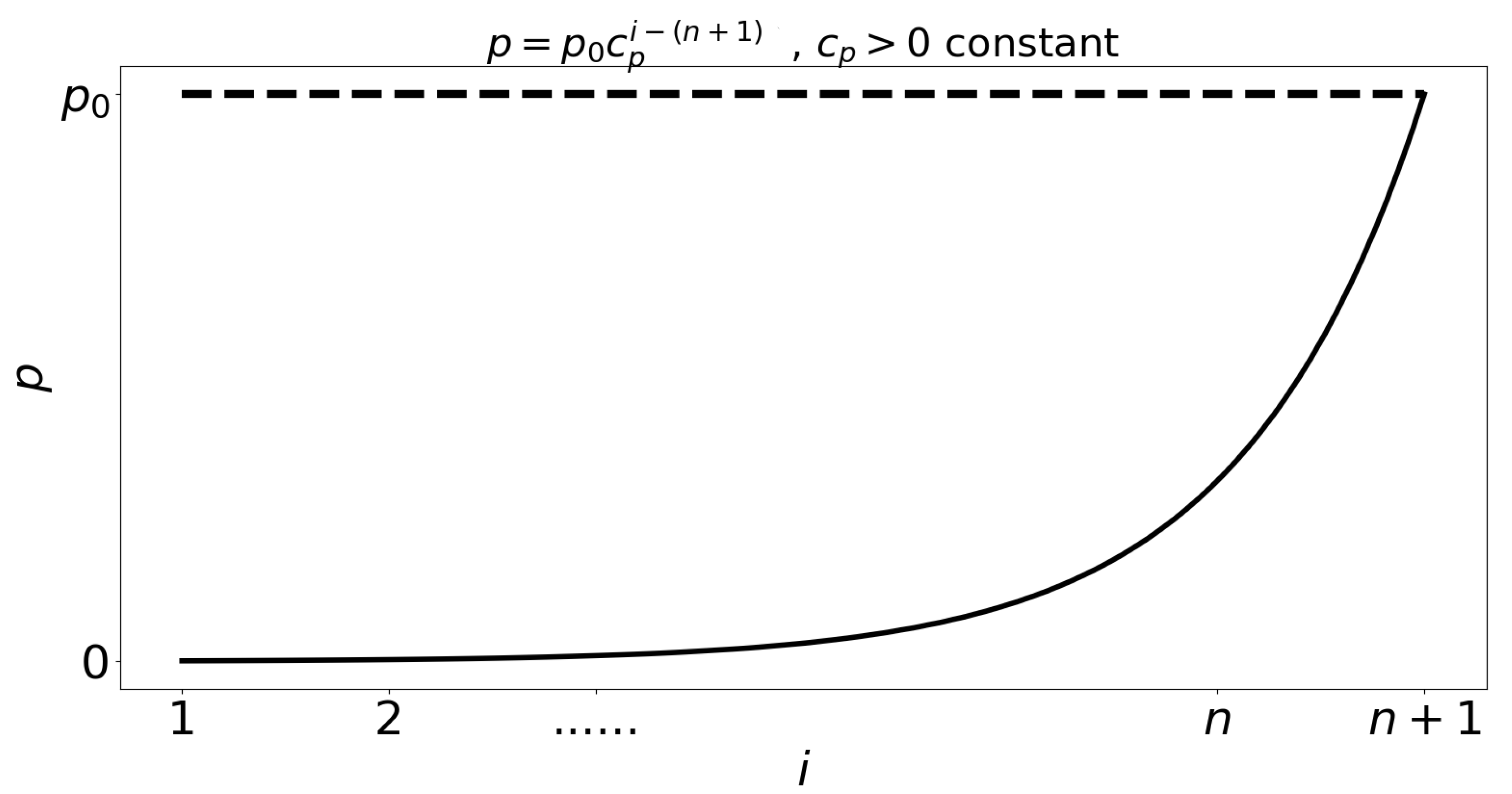
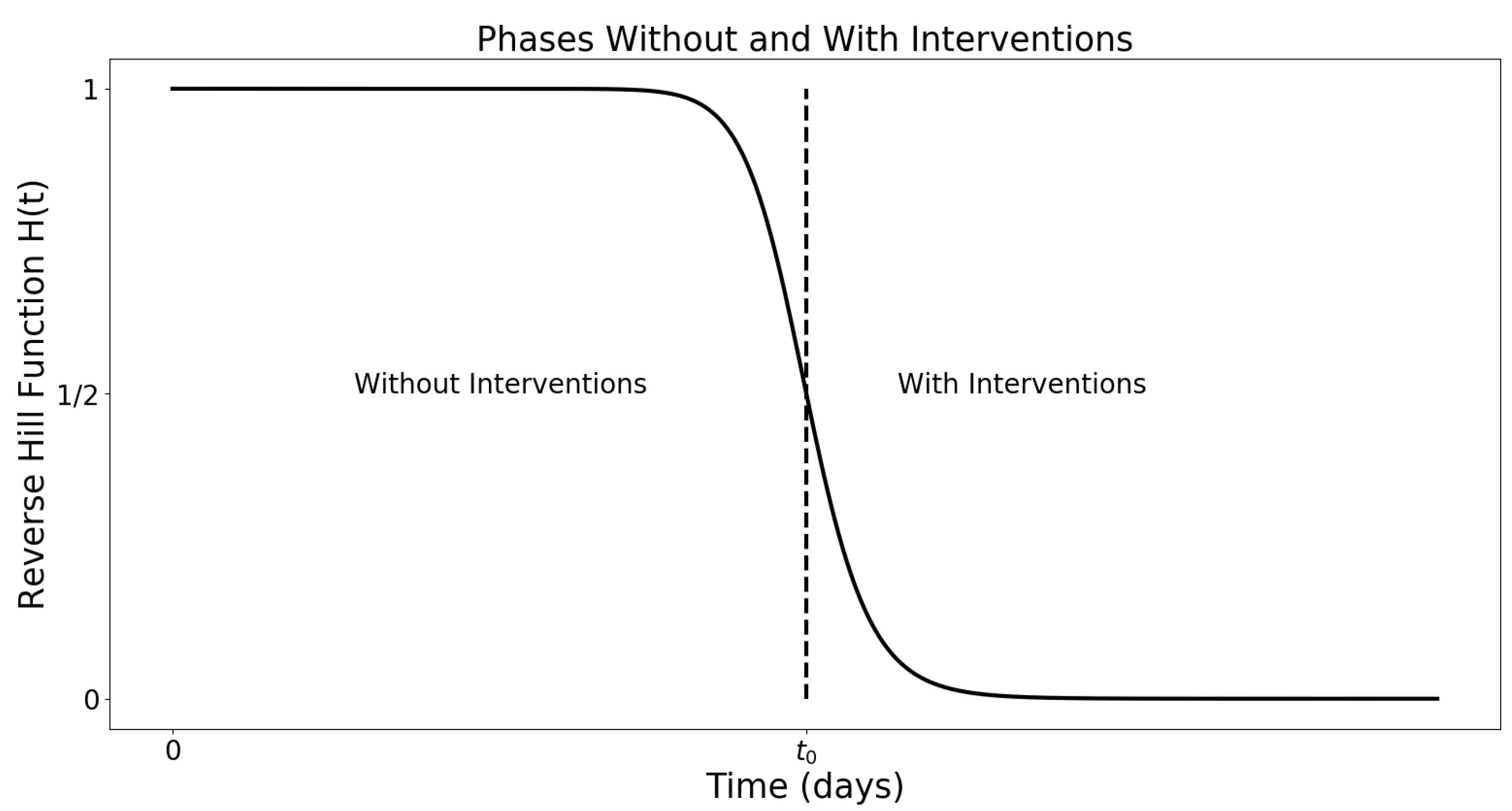
- Individuals infected by symptomatic individuals immediately become symptomatic without passing through an asymptomatic stage, whereas individuals infected by asymptomatic individuals become asymptomatic. This assumption is inspired by an exponential shedding dose-response curve, as illustrated in Figure 2.
- Individuals at earlier asymptomatic stages require further infection events to progress to the next asymptomatic stage, while individuals at later asymptomatic stages can automatically progress to the symptomatic stage.
- Individuals at earlier asymptomatic stages can only move onto the next asymptomatic stage if infected by those at higher asymptomatic stages of infection, or symptomatic individuals.
- Asymptomatic individuals can revert to earlier asymptomatic stages, but symptomatic individuals cannot revert to asymptomatic infection.
- For simplicity, we assume that pathogen mutations are not included, and thus, disease properties such as transmission, aggressivity and mortality remain unchanged in time. We also do not consider the intrinsic potential of the pathogen to lay dormant within the host, and assume that the pathogen is always active and able to infect.
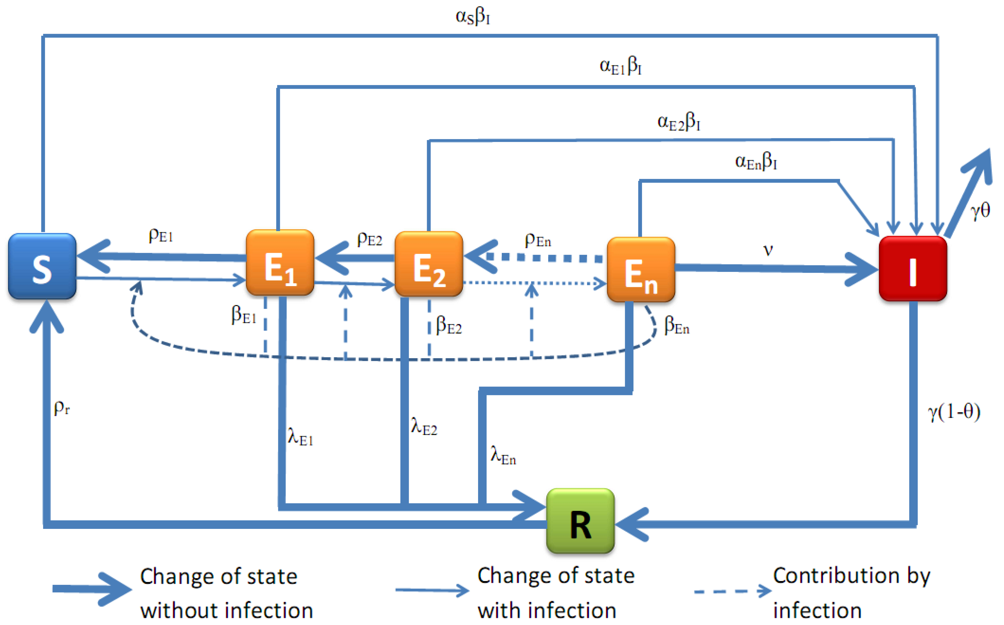
2.1. Model Presentation
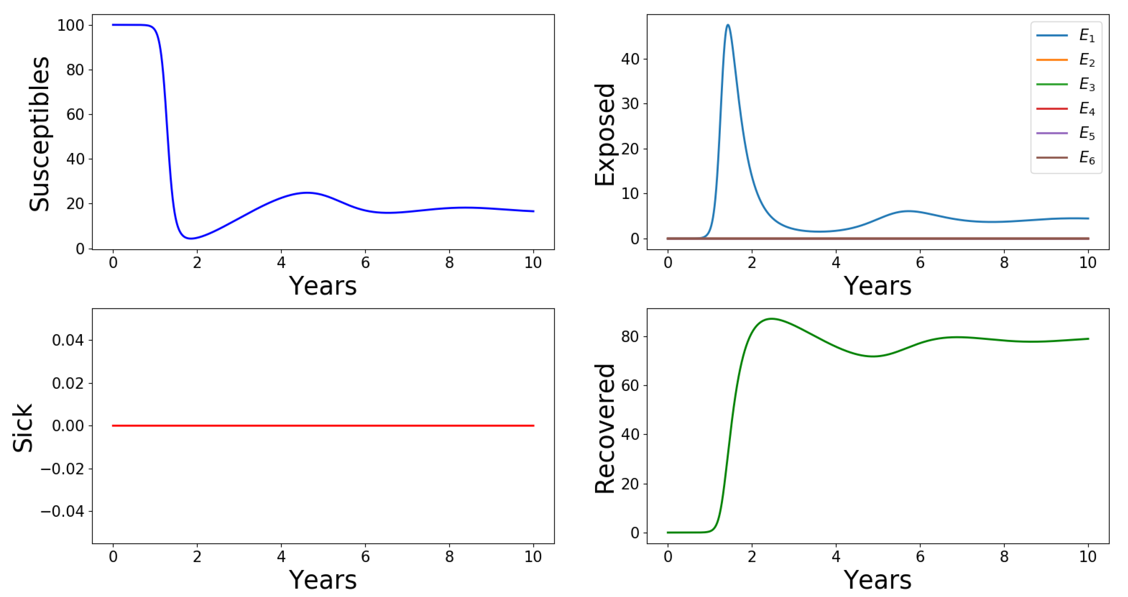
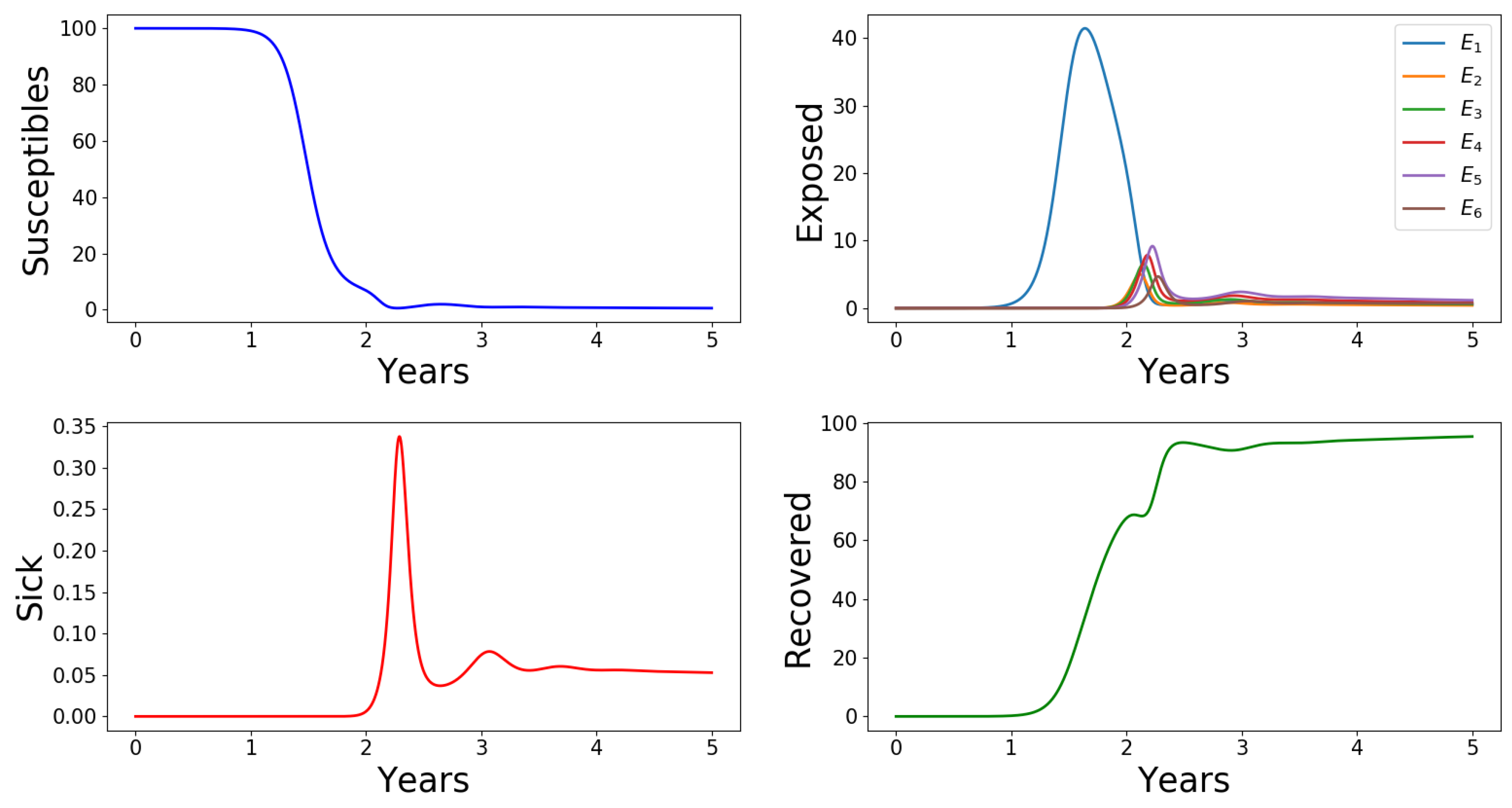
2.2. Numerical Results
3. Discussion and Conclusion
Author Contributions
Funding
Acknowledgments
Conflicts of Interest
Appendix A. Existence of Oscillatory Outbreak Equilibrium Points
Appendix A.1. Local Stability Analysis of Disease-Free Equilibrium
Appendix A.2. Parameters Estimation
- (a)
- The rates of transmission from asymptomatic and symptomatic individuals are related (increasing one necessarily increases the other, for example).
- (b)
- The rate of waning immunity from R is related to the rate of loss of infectiousness of s.
- (c)
- As individuals progress through asymptomatic classes , their susceptibility, transmissibility, rate of loss of infectiousness, and rate of gain of immunity all increase.
Appendix A.2.1. Estimate for b and μ:
Appendix A.2.2. Estimate for βI and , i = 1,2,…,n:
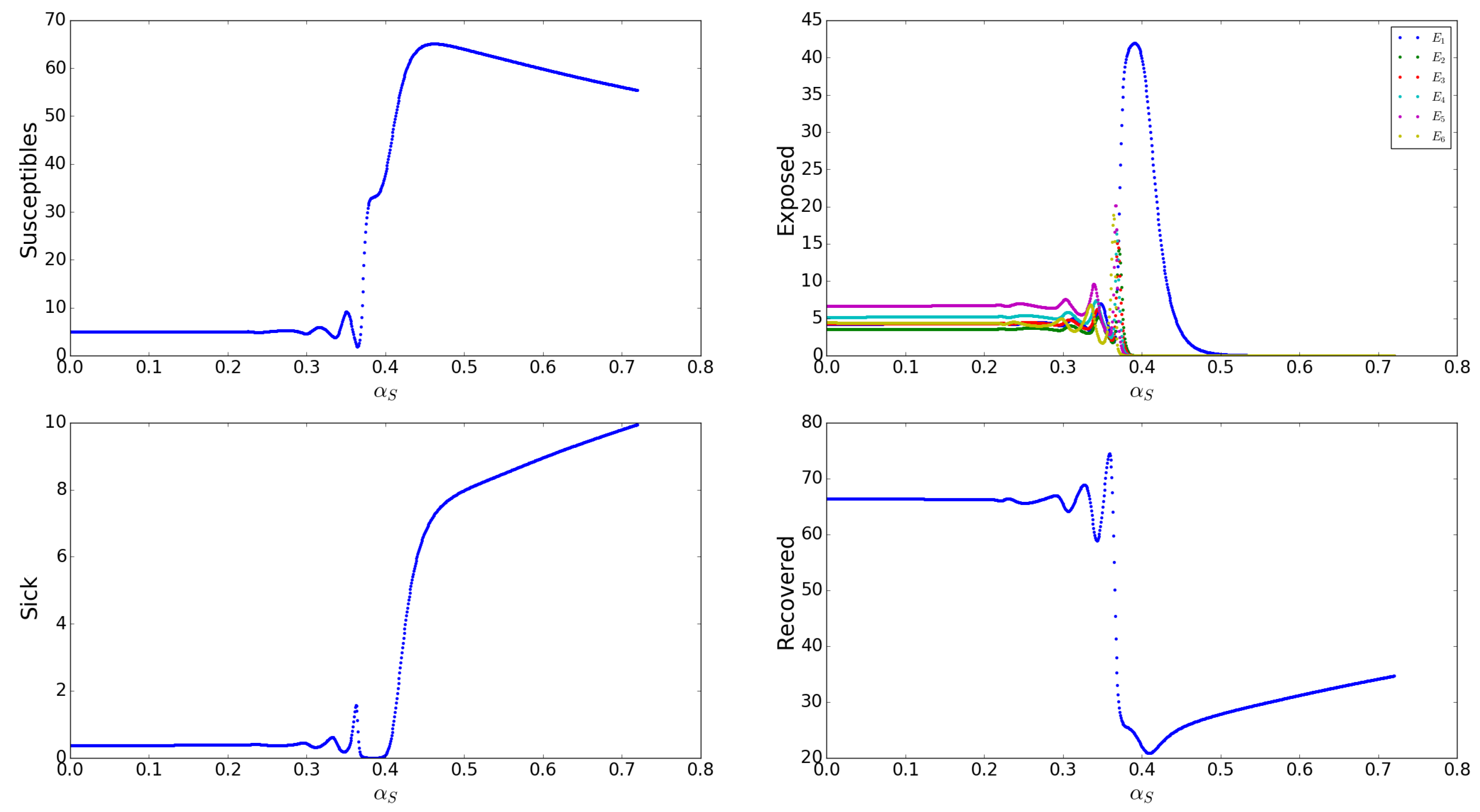
Appendix A.2.3. Estimate for αS and , i = 1,2,…,n:
Appendix A.2.4. Estimate for , i = 1,2,…,n:
Appendix A.2.5. Estimate for , i = 1,2,…,n:
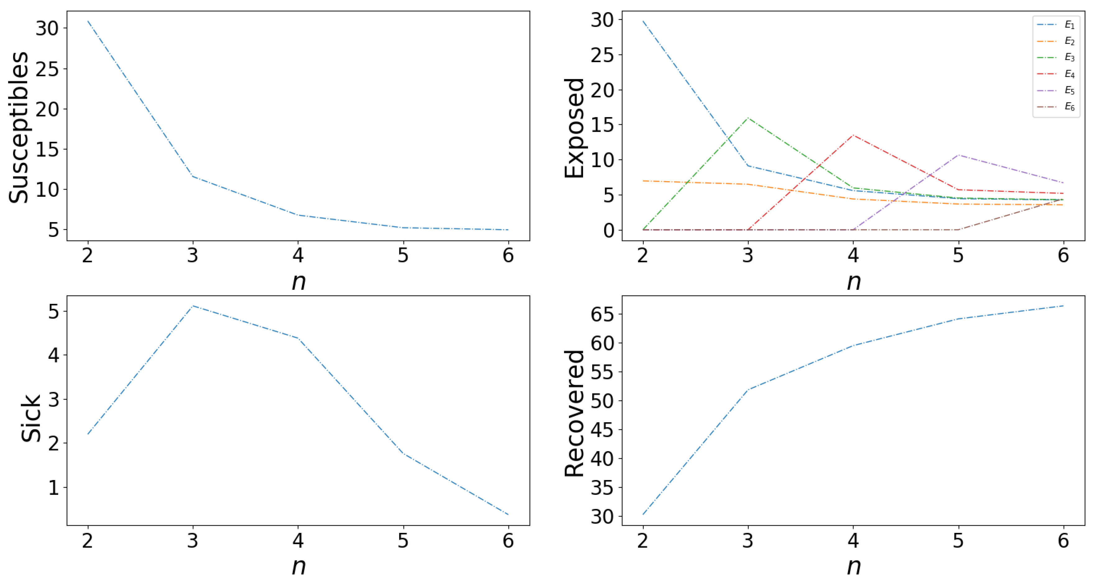
Appendix A.2.6. Effects of Number of Asymptomatic Cases, n

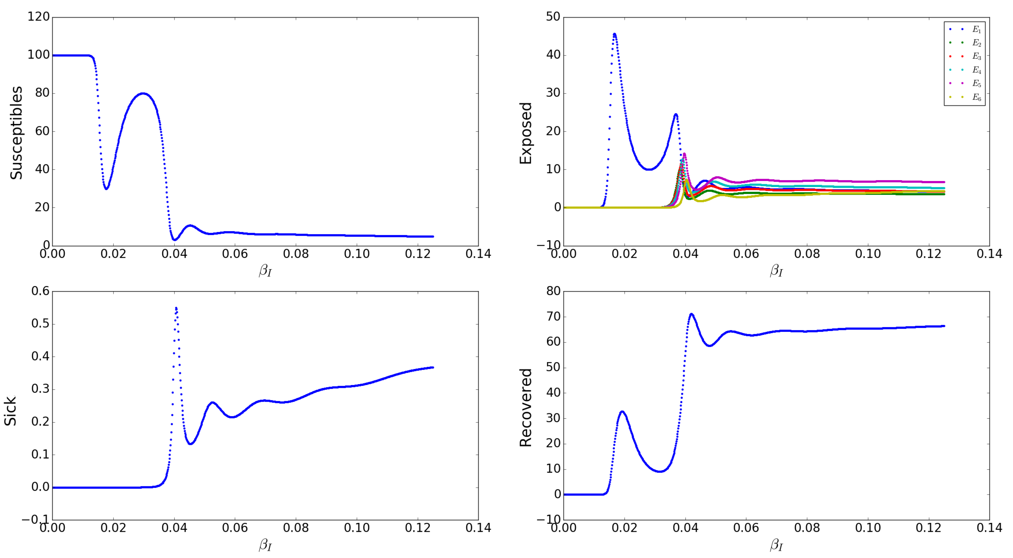
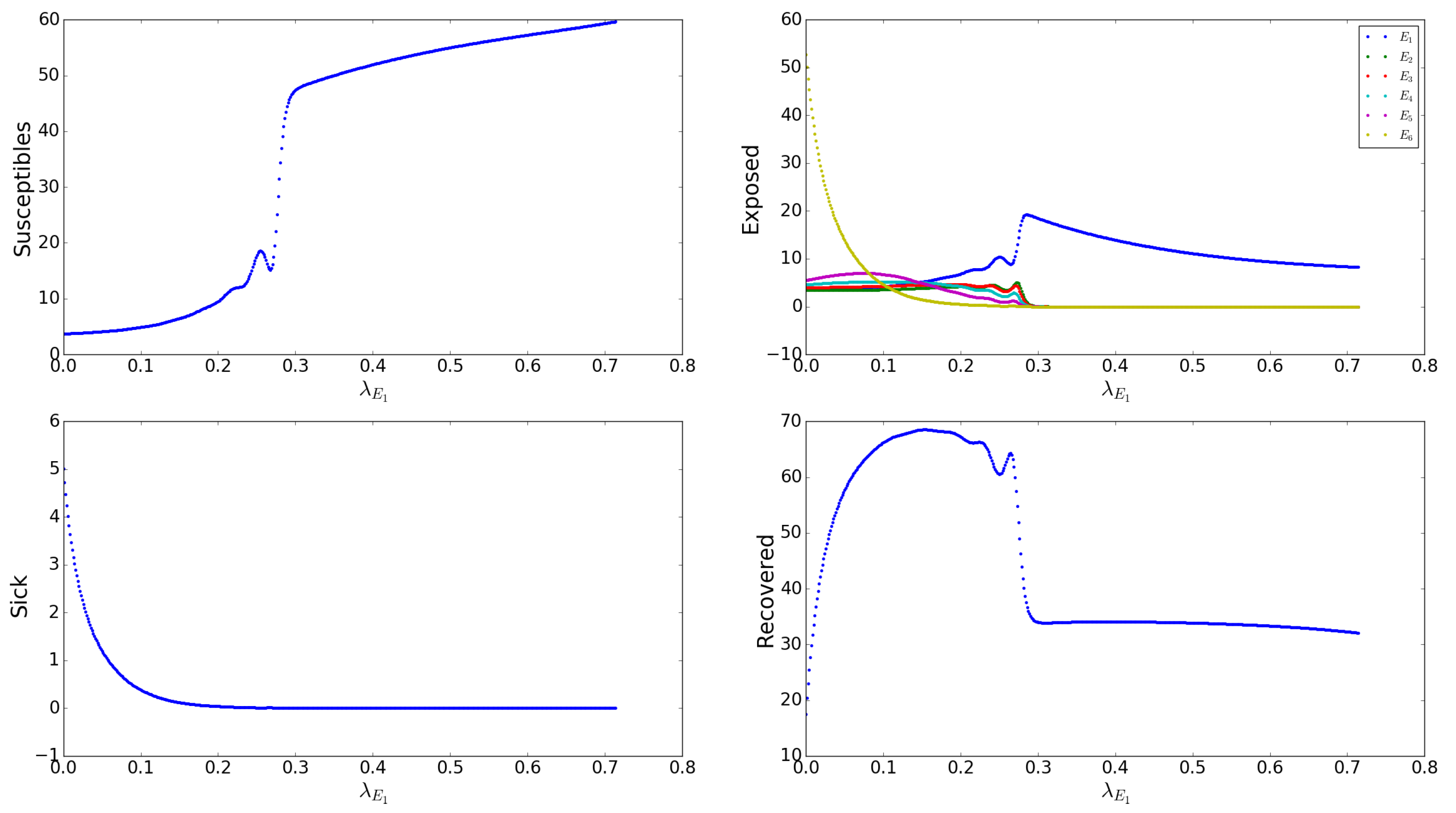
Appendix A.2.7. Effects of the Asymptomatic Transmission Rates s

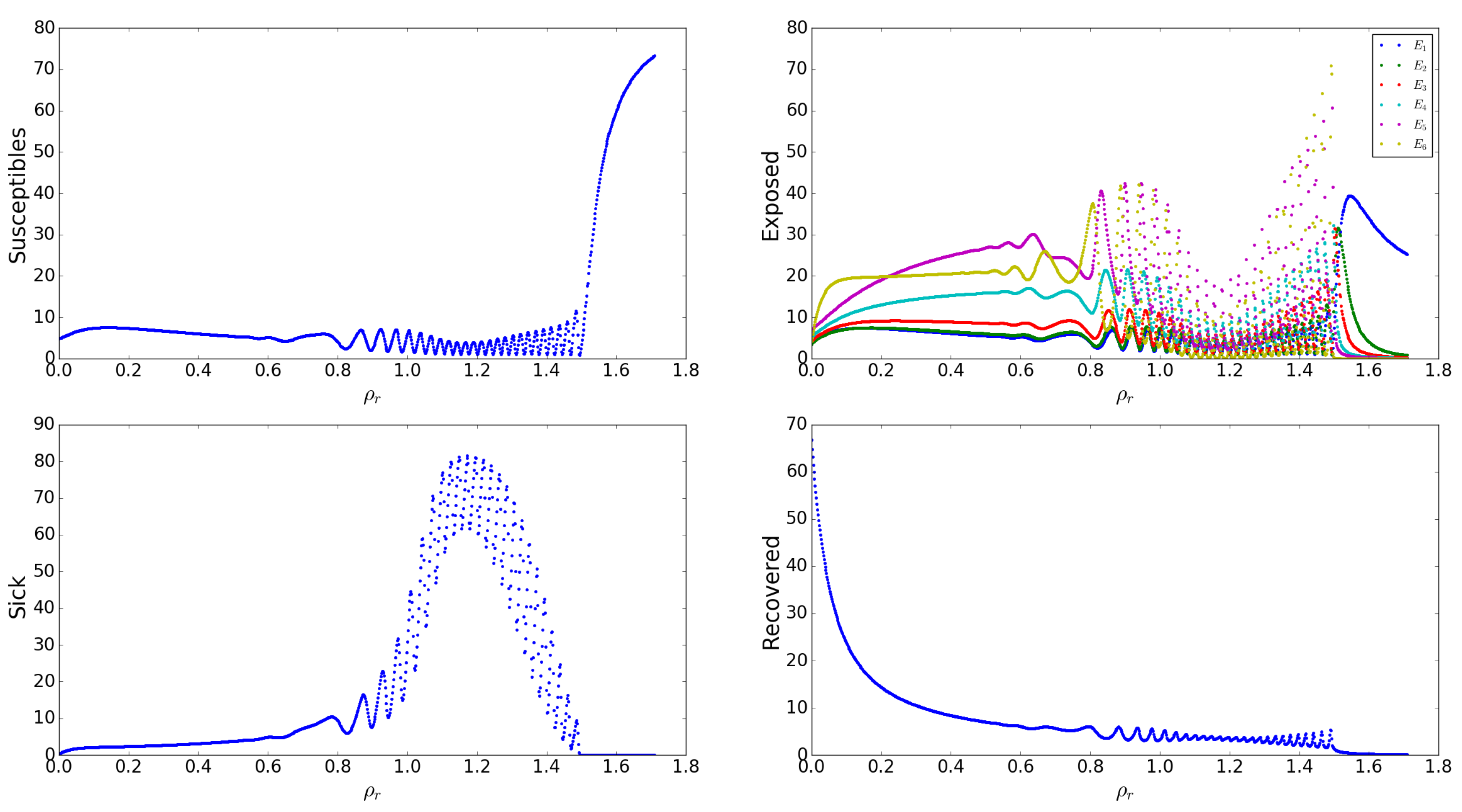
Appendix A.2.8. Effects of the Loss/Recovery of Asymptomatic Infection Rates s

Appendix A.2.9. Effects of the Clinical Transmission Rates s

Appendix A.2.10. Effects of the Gain of Immunity Rates by Asymptomatic Humans, s

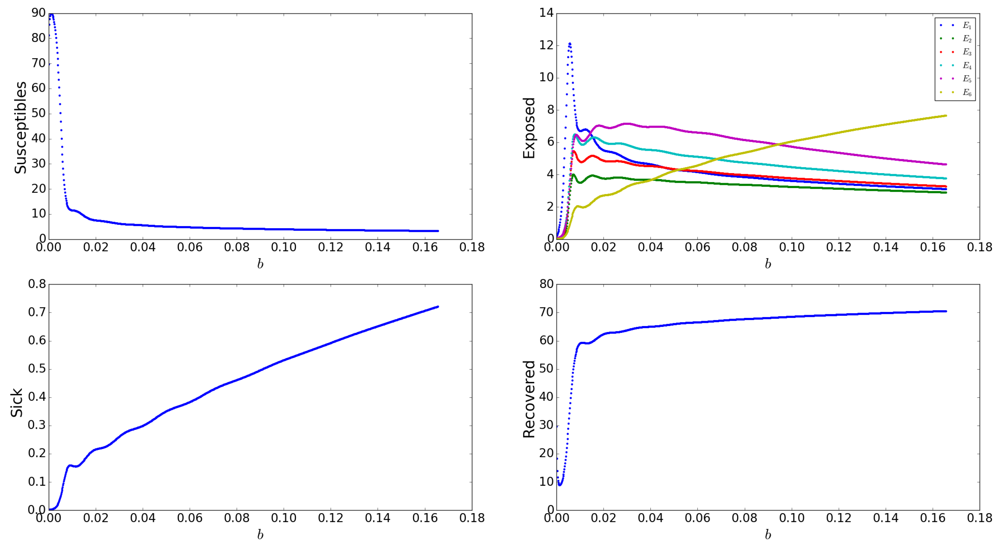
Appendix A.2.11. Effects of Birth Rate, b

Appendix B. Ebola (DRC 1995) and COVID-19 (New York 2020)

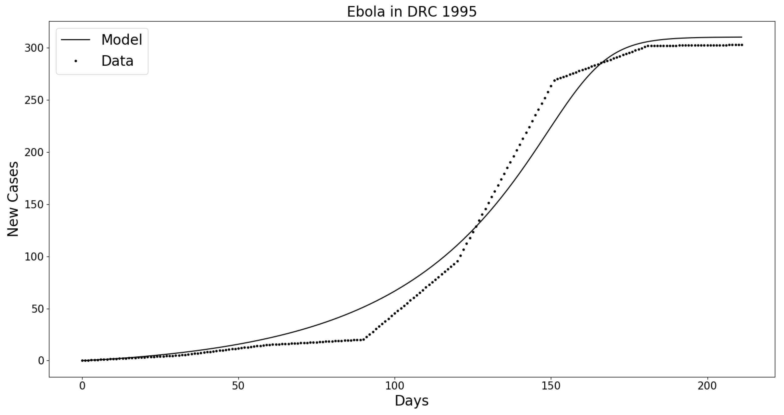
Appendix B.1. Ebola in the Democratic Republic of Congo (DRC) 1995

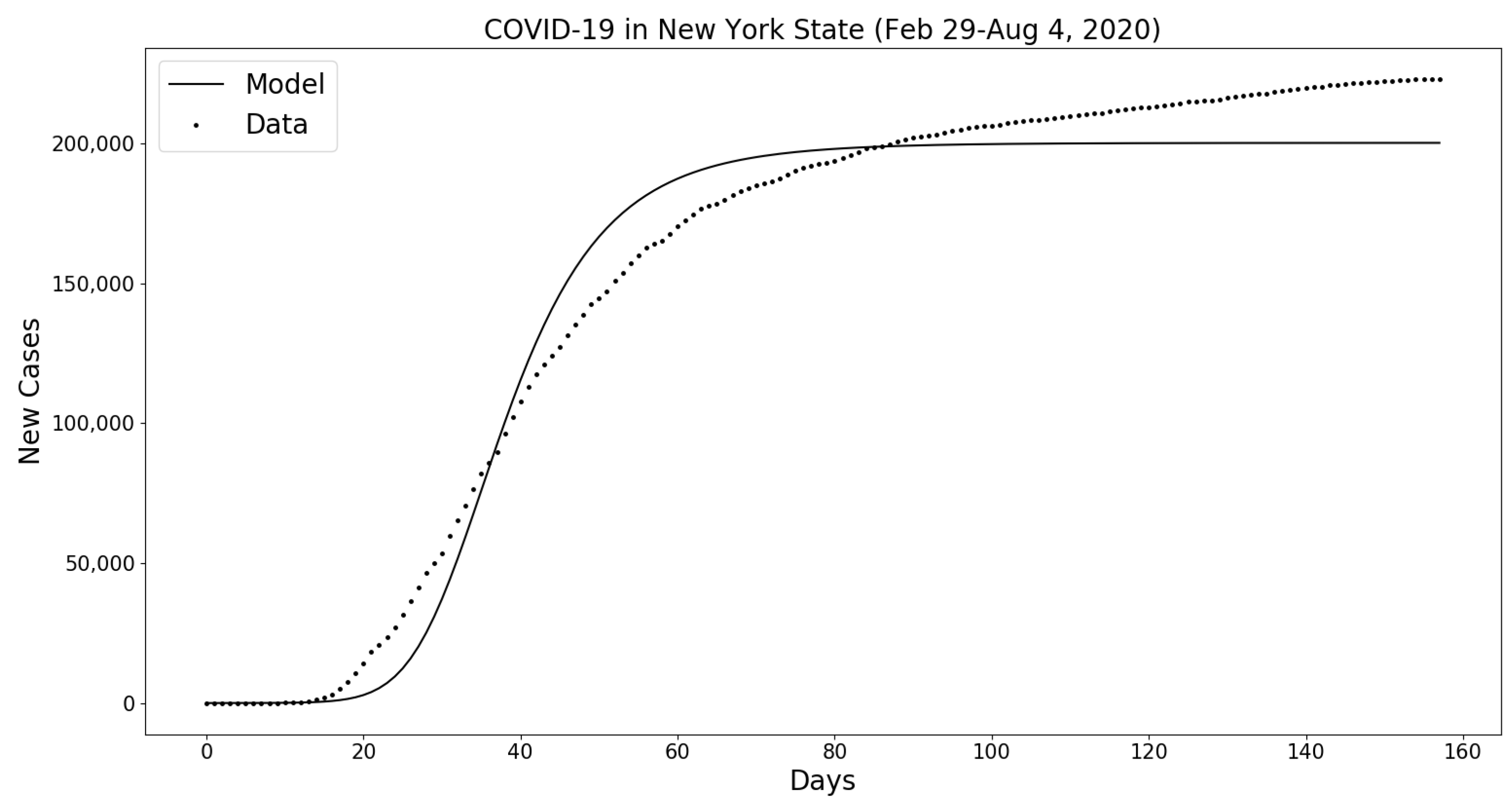
Appendix B.2. COVID-19 in New York State (February 29–4 August 2020)

References
- Grais, R.; Conlan, A.; Ferrari, M.; Djibo, A.; Le Menach, A.; Bjørnstad, O.; Grenfell, B. Time is of the essence: Exploring a measles outbreak response vaccination in Niamey, Niger. J. R. Soc. Interface 2008, 5, 67–74. [Google Scholar] [CrossRef] [Green Version]
- Rotz, L.D.; Hughes, J.M. Advances in detecting and responding to threats from bioterrorism and emerging infectious disease. Nat. Med. 2004, 10, S130–S136. [Google Scholar] [CrossRef]
- Moore, K. Real-time syndrome surveillance in Ontario, Canada: The potential use of emergency departments and Telehealth. Eur. J. Emerg. Med. 2004, 11, 3–11. [Google Scholar] [CrossRef] [PubMed]
- Wang, S.X.; Li, Y.; Sun, B.; Zhang, S.; Zhao, W.; Wei, M.; Chen, K.; Zhao, X.; Zhang, Z.; Krahn, M.; et al. The SARS outbreak in a general hospital in Tianjin, China–the case of super-spreader. Epidemiol. Infect. 2006, 134, 786–791. [Google Scholar] [CrossRef] [PubMed]
- Shapiro, M.; London, B.; Nigri, D.; Shoss, A.; Zilber, E.; Fogel, I. Middle East respiratory syndrome coronavirus: Review of the current situation in the world. Disaster Mil. Med. 2016, 2, 9. [Google Scholar] [CrossRef] [PubMed] [Green Version]
- Grassly, N.C.; Fraser, C. Seasonal infectious disease epidemiology. Proc. R. Soc. Lond. B Biol. Sci. 2006, 273, 2541–2550. [Google Scholar] [CrossRef] [PubMed] [Green Version]
- Banu, S.; Hu, W.; Hurst, C.; Tong, S. Dengue transmission in the Asia-Pacific region: Impact of climate change and socio-environmental factors. Trop. Med. Int. Health 2011, 16, 598–607. [Google Scholar] [CrossRef] [PubMed]
- Kitron, U. Landscape ecology and epidemiology of vector-borne diseases: Tools for spatial analysis. J. Med. Entomol. 1998, 35, 435–445. [Google Scholar] [CrossRef]
- Bansal, S.; Read, J.; Pourbohloul, B.; Meyers, L.A. The dynamic nature of contact networks in infectious disease epidemiology. J. Biol. Dyn. 2010, 4, 478–489. [Google Scholar] [CrossRef]
- Recker, M.; Blyuss, K.B.; Simmons, C.P.; Hien, T.T.; Wills, B.; Farrar, J.; Gupta, S. Immunological serotype interactions and their effect on the epidemiological pattern of dengue. Proc. R. Soc. Lond. B Biol. Sci. 2009, 276, 2541–2548. [Google Scholar] [CrossRef]
- Boerlijst, M.C.; Van Ballegooijen, W.M. Spatial pattern switching enables cyclic evolution in spatial epidemics. PLoS Comput. Biol. 2010, 6, e1001030. [Google Scholar] [CrossRef] [PubMed] [Green Version]
- Gandhi, M.; Yokoe, D.S.; Havlir, D.V. Asymptomatic Transmission, the Achilles’ Heel of Current Strategies to Control Covid-19. N. Engl. J. Med. 2020, 382, 2158–2160. [Google Scholar] [CrossRef] [PubMed]
- Huff, H.V.; Singh, A. Asymptomatic Transmission During the Coronavirus Disease 2019 Pandemic and Implications for Public Health Strategies. Clin. Inf. Dis. 2020, 654, 1–5. [Google Scholar] [CrossRef] [PubMed]
- Chrisholm, R.H.; Campbell, P.T.; Wu, Y.; Tong, S.Y.C.; McVernon, J.; Geard, N. Implications of asymptomatic carriers for infectious disease transmission and control. R. Soc. Open. Sci. 2018, 5, 1–13. [Google Scholar]
- Bellan, S.E. Ebola control: Effect of asymptomatic infection and acquired immunity. Lancet 2014, 384, 1499–1500. [Google Scholar] [CrossRef] [Green Version]
- Attenborough, T. Modelling the Ebola Outbreak in West Africa and Community Responses. Available online: https://www.ucl.ac.uk/~ucbptch/miniproject3TA.pdf (accessed on 15 April 2015).
- Liu, Z.; Magal, P.; Seydi, O.; Webb, G. Understanding Unreported Cases in the COVID-19 Epidemic Outbreak in Wuhan, China, and the Importance of Major Public Health Interventions. Biology 2020, 9, 50. [Google Scholar] [CrossRef] [PubMed] [Green Version]
- Khyar, O.; Allali, K. Global dynamics of a multi-strain SEIR epidemic model with general incidence rates: Application to COVID-19 pandemic. Nonlinear Dyn. 2020, 102, 1–21. [Google Scholar] [CrossRef] [PubMed]
- Bentaleb, D.; Amine, S. Lyapunov function and global stability for a two-strain SEIR model with bilinear and non-monotone incidence. Int. J. Biomath. 2019, 12. [Google Scholar] [CrossRef]
- Tang, Y.; Xiao, D.; Zhang, W.; Zhu, D. Dynamics of Epidemic models with Asymptomatic Infection and Seasonal Succession. Math. Biosci. Eng. 2017, 314, 1407–1424. [Google Scholar] [CrossRef]
- Ansumali, S.; Kaushal, S.; Kumar, A.; Prakash, M.K.; Vidyasagar, M. Modelling a pandemic with asymptomatic patients, impact of lockdown and herd immunity, with applications to SARS-CoV-2. Annu. Rev. Control 2020, 1–55. [Google Scholar] [CrossRef]
- Aguilar, J.B.; Gutierrez, J.B. An Epidemiological Model of Malaria Accounting for Asymptomatic Carriers. Bull. Math. Biol. 2020, 82, 1–55. [Google Scholar] [CrossRef] [PubMed] [Green Version]
- Schaffner, D.W.; Bowman, J.P.; English, D.J.; Fischler, G.E.; Fuls, J.L.; Krowka, J.F.; Kruszewski, F.H. Quantitative microbial risk assessment of antibacterial hand hygiene products on risk of shigellosis. J. Food Prot. 2014, 77, 574–582. [Google Scholar] [CrossRef] [PubMed]
- Popovich, K.J.; Hota, B.; Aroutcheva, A.; Kurien, L.; Patel, J.; Lyles-Banks, R.; Grasso, A.E.; Spec, A.; Beavis, K.G.; Hayden, M.K.; et al. Community-associated methicillin-resistant Staphylococcus aureus colonization burden in HIV-infected patients. Clin. Infect. Dis. 2013, 56, 1067–1074. [Google Scholar] [CrossRef] [PubMed] [Green Version]
- Bichara, D.; Kang, Y.; Castillo-Chavez, C.; Horan, R.; Perrings, C. SIS and SIR epidemic models under virtual dispersal. Bull. Math. Biol. 2015, 77, 2004–2034. [Google Scholar] [CrossRef] [PubMed]
- Chowell, D.; Hengartner, N.W.; Castillo–Chavez, C.; Fenimore, P.W.; Hyman, J.M. The basic reproductive number of Ebola and the effects of public health measures: The cases of Congo and Uganda. J. Theor. Biol. 2004, 229, 119–126. [Google Scholar] [CrossRef] [Green Version]
- Chowell, D.; Castillo-Chavez, C.; Krishna, S.; Qiu, X.; Anderson, K.S. Modeling the effect of early detection of Ebola. Lancet Infect. Dis. 2015, 15, 148–149. [Google Scholar] [CrossRef]
- Drake, J.M.; Bakach, I.; Just, M.R.; O’Regan, S.M.; Gambhir, M.; Fung, I.C. Transmission Models of Historical Ebola Outbreaks. Emerg. Inf. Dis. 2015, 21, 1447–1450. [Google Scholar] [CrossRef] [Green Version]
- Ngwa, G.A.; Teboh–Ewungkem, M. A Mathematical Model with Quarantine States for the Dynamics of Ebola Virus Disease in Human Populations. Comput. Math. Methods Med. 2016, 2016, 1–29. [Google Scholar] [CrossRef] [Green Version]
- Webb, G.; Browne, C.; Huo, X.; Seydi, O.; Seydi, M.; Magal, P. A Model of the 2014 Ebola Epidemic in West Africa with Contact Tracing. PLoS Curr. Outbreaks 2015, 7, 1–20. [Google Scholar] [CrossRef]
- Caugant, D.A.; Maiden, M.C. Meningococcal carriage and disease—population biology and evolution. Vaccine 2009, 27, B64–B70. [Google Scholar] [CrossRef] [Green Version]
- Siewe, N.; Yakubu, A.A.; Satoskar, A.R.; Friedman, A. Immune Response to Infection by Leishmania: A Mathematical Model. Math. Biosci. 2016, 276, 28–43. [Google Scholar] [CrossRef] [PubMed]
- Castillo–Chavez, C.; Barley, K.; Bichara, D.; Chowell, D.; Diaz Herrera, E.; Espinoza, B.; Moreno, V.; Towers, S.; Yong, K.E. Modeling Ebola at the Mathematical and Theoretical Biology Institute (MTBI). Not. AMS 2016, 63, 366–371. [Google Scholar] [CrossRef]
- Alpren, C.; Sloan, M.; Boegler, K.A.; Martin, D.W.; Ervin, E.; Washburn, F.; Rickert, R.; Singh, T.; Redd, J.T. Intereagency Investigation Team. Ebola Virus Disease Cluster—Northern Sierra Leone, January 2016. MMWR 2016, 65, 681–682. [Google Scholar] [PubMed] [Green Version]
- Heung, N.H.L.; Xu, C.; Ip, D.K.M.; Cowling, B.J. The fraction of influenza virus infections that are asymptomatic: A systematic review and meta-analysis. Epidemiology 2015, 26, 862–872. [Google Scholar]
- Glynn, J.R.; Bower, H.; Johnson, S.; Houlihan, C.F.; Montesano, C.; Scott, J.T.; Semple, M.G.; Bangura, M.S.; Kamara, A.J.; Kamara, O.; et al. Asymptomatic infection and unrecognised Ebola virus disease in Ebola-affected households in Sierra Leone: A cross-sectional study using a new non-invasive assay for antibodies to Ebola virus. Lancet Inf. Dis. 2017, 17, 645–653. [Google Scholar] [CrossRef] [Green Version]
- Tasca, K.I.; Correa, C.R.; Caleffi, J.T.; Mendes, M.B.; Gatto, M.; Manfio, V.M.; Cavassan de Camargo, C.; Tavares, F.C.; Biasin, M.; Rosário de Souza, L.D. Asymptomatic HIV People Present Different Profiles of sCD14, sRAGE, DNA Damage, and Vitamins, according to the Use of cART and CD4+ T Cell Restoration. J. Immunol. Res. 2018, 2018, 1–11. [Google Scholar] [CrossRef] [Green Version]
- Mizumoto, K.; Kagaya, K.; Zarebski, A.; Chowell, G. Asymptomatic HIV People Present Different Profiles of sCD14, sRAGE, DNA Damage, and Vitamins, according to the Use of cART and CD4+ T Cell Restoration. Eurosurveillance 2020, 25, 1–5. [Google Scholar]
- Gupta, R.K.; Sakhuja, P.; Majumdar, K.; Ali, S.; Srivastava, S.; Sachdeva, S.; Sharma, B.C.; Puri, A.S. Incidentally detected asymptomatic hepatitis C virus infection with significant fibrosis: Possible impacts on management. Indian J. Pathol. Microbiol. 2018, 61, 345–349. [Google Scholar] [CrossRef]
- Mertz, G.J. Asymptomatic Shedding of Herpes Simplex Virus 1 and 2: Implications for Prevention of Transmission. J. Inf. Dis. 2008, 198, 1098–1100. [Google Scholar] [CrossRef] [Green Version]
- Hauck, F.R.; Neese, B.H.; Panchal, A.S.; El-Amin, W. Identification and Management of Latent Tuberculosis Infection. Am. Fam. Physician 2009, 79, 879–886. [Google Scholar]
- Li, M.; Song, Y.; Li, B.; Wang, Z.; Yang, R.; Jiang, L.; Yang, R. Asymptomatic Yersinia pestis infection, China. Emerg. Infect. Dis. 2005, 11, 1494–1496. [Google Scholar] [CrossRef] [PubMed]
- WHO. Ebola Virus Disease Update—West Africa. Emergencies Prep. Response. Disease Outbreak News. Available online: https://www.who.int/csr/don/2014_07_10_ebola/en/ (accessed on 10 July 2014).
- CDC. The Road to Zero: CDC’s Response to the West African Ebola Epidemic, 2014–2015. 9 July 2015. [Google Scholar]
- Statisques Mondiales Taux de Natalite par Pays 2008–2015 (Par Ordre Alphabetique Des Pays). Available online: https://www.statistiques-mondiales.com/ (accessed on 18 September 2019).
- Siewe, N.; Lenhart, S.; Yakubu, A. Ebola outbreaks and international travel restrictions: Case studies of Central and West Africa regions. J. Biol. Syst. 2020, 28, 431–452. [Google Scholar] [CrossRef]
- Khan, A.S.; Tshioko, F.K.; Heymann, D.L.; Guenno, B.L.; Nabeth, P.; Kerstiens, B.; Fleerackers, Y.; Kilmarx, P.H.; Rodier, G.R.; Nkulu, O.; et al. The reemergence of Ebola hemorrhagic fever, Democratic Republic of the Congo, 1995. J. Inf. Dis. 1999, 179, S76–S86. [Google Scholar] [CrossRef] [PubMed] [Green Version]
- New York City Health. Available online: COVID-19Data.https://www1.nyc.gov/site/doh/covid/covid-19-data.page (accessed on 6 August 2020).
- The New York Times. New York Covid Map and Case Count. Available online: https://www.nytimes.com/interactive/2020/us/new-york-coronavirus-cases.html (accessed on 6 August 2020).
- NYC Health. Annual Vital Statistics Data Show Fewer Premature Deaths and Fewer Births in New York City in 2017. Available online: [email protected] (accessed on 6 August 2020).
- New York State Community Health Indicator Reports (CHIRS). Health Status and Social Determinants of Health. Available online: [email protected] (accessed on 6 August 2020).


| Variables | Descriptions |
|---|---|
| S | number of susceptible humans |
| s | numbers of asymptomatic (latent) humans, of various stages |
| I | number of infected humans who show clinical signs |
| R | number of recovered humans |
| Parameters | Descriptions | Values | Sources |
|---|---|---|---|
| , s | weights of infectiousness of S and s by contact with I | 0.036, | Appendix A.2.3 |
| b | rate of recruitment of humans | per day | Appendix A.2.1 |
| , s | rates of transmission by contact with I and s | 0.125, per day | Appendix A.2.2 |
| rate of wane of immunity of R | per day | Appendix A.2.5 | |
| s | rates of loss of infectiousness of s | per day | Appendix A.2.5 |
| s | rates of gain of immunity of s | per day | Appendix A.2.4 |
| rate of removal from sick class I | 0.167 per day | [33] | |
| rate of transition from to I | 0.05 per day | assumed | |
| natural death rate of humans | per day | Appendix A.2.1 | |
| fraction of humans I who die | 0.7 | [33] | |
| n | number of asymptomatic stages | 6 | assumed |
| number of asymptomatic stages that do not transit to higher infection stage “naturally” | 1 | assumed | |
| Total initial population size | 11.5 million | assumed |
Publisher’s Note: MDPI stays neutral with regard to jurisdictional claims in published maps and institutional affiliations. |
© 2020 by the authors. Licensee MDPI, Basel, Switzerland. This article is an open access article distributed under the terms and conditions of the Creative Commons Attribution (CC BY) license (http://creativecommons.org/licenses/by/4.0/).
Share and Cite
Siewe, N.; Greening, B., Jr.; Fefferman, N.H. Mathematical Model of the Role of Asymptomatic Infection in Outbreaks of Some Emerging Pathogens. Trop. Med. Infect. Dis. 2020, 5, 184. https://0-doi-org.brum.beds.ac.uk/10.3390/tropicalmed5040184
Siewe N, Greening B Jr., Fefferman NH. Mathematical Model of the Role of Asymptomatic Infection in Outbreaks of Some Emerging Pathogens. Tropical Medicine and Infectious Disease. 2020; 5(4):184. https://0-doi-org.brum.beds.ac.uk/10.3390/tropicalmed5040184
Chicago/Turabian StyleSiewe, Nourridine, Bradford Greening, Jr., and Nina H. Fefferman. 2020. "Mathematical Model of the Role of Asymptomatic Infection in Outbreaks of Some Emerging Pathogens" Tropical Medicine and Infectious Disease 5, no. 4: 184. https://0-doi-org.brum.beds.ac.uk/10.3390/tropicalmed5040184