Cosmological Constant from Condensation of Defect Excitations


Perimeter Institute for Theoretical Physics, 31 Caroline Street North, Waterloo, ON N2L 2Y5, Canada
Universe 2018, 4(7), 81; https://0-doi-org.brum.beds.ac.uk/10.3390/universe4070081
Submission received: 30 May 2018
/
Revised: 9 July 2018
/
Accepted: 11 July 2018
/
Published: 19 July 2018
(This article belongs to the Special Issue Loop Quantum Gravity and Non-Perturbative Approaches to Quantum Cosmology)
Abstract
:A key challenge for many quantum gravity approaches is to construct states that describe smooth geometries on large scales. Here we define a family of -dimensional quantum gravity states which arise from curvature excitations concentrated at point like defects and describe homogeneously curved geometries on large scales. These states represent therefore vacua for three-dimensional gravity with different values of the cosmological constant. They can be described by an anomaly-free first class constraint algebra quantized on one and the same Hilbert space for different values of the cosmological constant. A similar construction is possible in four dimensions, in this case the curvature is concentrated along string-like defects and the states are vacua of the Crane-Yetter model. We will sketch applications for quantum cosmology and condensed matter.
1. Introduction
Three-dimensional gravity with Euclidean signature and positive cosmological constant can be described by the Turaev-Viro partition function [1,2] with a quantum deformed structure group . The Turaev-Viro models are defined for triangulated three-dimensional manifolds, the partition function is however invariant under changes of the (bulk) triangulation. Here is the so-called level which determines the quantum deformation parameter . The value of the cosmological constant is encoded in the level
with G the three-dimensional Newton’s constant. We thus have a quantized cosmological constant .
An earlier variant of the Turaev-Viro model is the Ponzano-Regge model [3], which describes Euclidean three-dimensional gravity without a cosmological constant. The Ponzano-Regge model can also be understood as a zero-coupling limit of three-dimensional lattice gauge theory with structure group.
That these models do in fact describe gravity can be shown by a semi-classical analysis of their amplitudes [4,5,6,7]. This analysis reproduces the Regge action, which describes discretized gravity based on flat [8] or homogeneously curved tetrahedra [9,10]. Furthermore, both the Ponzano-Regge and Turaev-Viro (henceforth TV) models are topological theories, as is three-dimensional gravity. This is also the case for three-dimensional Regge gravity, if one uses homogeneously curved tetrahedra for the theory with cosmological constant [9].
The dynamics of the Turaev-Viro model can also be described in a canonical form, e.g., with loop quantum gravity techniques [11,12,13,14] or within the string net formalism [15,16,17,18,19,20]. By choosing a adapted vacuum state for the loop quantum gravity Hilbert space—instead of a vacuum peaked on flat geometries [21,22,23] or a totally degenerate geometry [24,25,26]—one can bring these two formulations together [20].
In the canonical formalism one distinguishes between the kinematics and dynamics. In the works cited above, the cosmological constant is already built into the kinematics, simplifying indeed enormously the imposition of the dynamics.
In this paper we show that one can separate kinematics and dynamics, that is express the dynamics and solutions for different cosmological constants in the same kinematical Hilbert space. This does in particular allow to express solutions for different cosmological constant, which are peaked on different values of the homogeneous curvature, in the same Hilbert space. A solution with a cosmological constant can then be analyzed with regard to the curvature excitations on top of a -vacuum. These are excitations which are also induced by massive (here spin-less) point particles. The vacuum can thus be understood to arise from a very particular superposition of such excited states.
This work does pick up on a research direction to derive the quantum group deformation from the imposition of the cosmological constant [9,27,28,29,30]. One main difficulty here is that as one is involving a discretization to define a diffeomorphism invariant dynamics, one encounters generically anomalies in the diffeomorphism constraint algebra [27,28] or covariantly, breaks diffeomorphism symmetry [31,32,33]. Here we will present an anomaly free quantization of the constraints defining the dynamics (for one of the allowed discrete values) in a kinematical Hilbert space associated to any allowed .
An alternative way to construct such quantizations which preserve diffeomorphism symmetry is to subject a given, not necessarily diffeomorphism invariant discrete theory, to a coarse graining flow. Each coarse graining step constructs an effective dynamics for a coarser lattice which reflects the dynamics of the finer lattice. Iterating the procedure, one is performing a refinement limit and thus reaches a fixed point of the coarse graining flow. One can then hope that diffeomorphism symmetry is restored in this limit [9,34,35,36,37,38,39].
This strategy has been proposed in [9] and has also been demonstrated to work for classical Regge calculus with a cosmological constant. It would be of course very useful to see that this can be extended to the quantum level, and this does indeed seem to be in reach [40]. This current work can be seen as a set–up for considering this coarse graining flow in a given Hilbert space. More generally, we could consider a microscopic gravitational Hamiltonian and subject it to a renormalization flow. The end points of these flows are fixed points that typically describe a topological phase. Depending on our initial choice of Hilbert space, given by the level , the possible fixed points do include 3D general relativity with positive discrete values for the cosmological constant described by levels k with . We can also consider a flow of the gravitational Hamiltonian driven by some external agent, e.g., matter content. In this context note that inside a fixed Hilbert space described by k, we can consider the flow from to , but also the flow from to , as long as .
In the discussion session we will further comment on possible phase transitions connected with this flow as well as describe further application of the framework presented here.
Outline of the paper: In the next Section 2 we will give a definition of the Turaev-Viro (TV) model and a related family of models. We will then follow up with a Hamiltonian description in Section 3. We will first introduce the string net framework that defines a physical Hilbert space associated to the TV model. We then define a kinematical Hilbert space by introducing punctures that can carry defect excitations and thus allow for a dynamics different from the TV model. The kinematical Hilbert spaces still carry a -dependent structure, but we will define an embedding of the -Hilbert space into the -Hilbert space for . Using the simplest example, namely the two-punctured sphere, we then give a detailed description of the framework in Section 4. In Section 5 we will consider general triangulations and show how to construct the various Hamiltonians, ribbon operators and - and -vacua in this case. This will also allow us to analyze the -vacua in terms of the excitations. We close with a discussion and outlook in Section 6. The Appendix A, Appendix B and Appendix C collect various more technical background material, in particular some essential definitions related to .
2. The Turaev-Viro Partition Function and Related Models
The TV model based on defines a partition function for 3D triangulations. The partition functions sums tetrahedral weights over labels associated to edges. These labels are given by irreducible representations (irreps) :
Here the amplitudes associated to the tetrahedra are given by
and is (one version of) the recoupling symbol (See Appendix A). The six irreps are associated to the six edges of the tetrahedron as shown in Figure 1.
The are the signed quantum dimension associated to the irreps j and appear in (2) as measure factors. Furthermore, the normalization in (2) depends only on the number of vertices where is the total quantum dimension of and is the number of vertices in the triangulation.
Note that as the tetrahedral amplitude is being given by an recoupling symbol it will only be non-vanishing if the following coupling conditions are satisfied for any of the triples of irreps labelling a triangle:
The TV partition function can also be defined for a triangulation with boundary—in this case the sum is only over the j’s associated to bulk edges. For boundary edges, one uses a measure factor (instead of ) and the normalization changes to
with the number of bulk vertices and the number of vertices in the boundary.
The partition function (2) is invariant under changes of the bulk triangulation and thus defines for closed manifolds a topological invariant. From this bulk invariance it also follows that for manifolds with boundary which are homomorphic to the partition function can be understood to act as a projector on the so-called kinematical boundary Hilbert space, which we will define in Section 3.2.
Thus, the partition function (2) has very special properties. We can consider this partition function as a very particular example of a family of models, which are of the same form as (2), e.g., can be written as
with some normalization factor , possibly depending on the number of vertices, tetrahedral amplitudes , which are functions of irreps assigned to the edges of this tetrahedron and weight factors associated to the edges. Here we will assume that the amplitude vanishes if the coupling conditions (4) are not satisfied. This will allow us to express these amplitudes as states in the kinematical boundary Hilbert space associated to the models.
We can now consider a renormalization flow of partition functions of the type (6). That is we glue the tetrahedra (or more general building blocks) to larger building blocks, integrate out the resulting bulk variables and obtain effective amplitudes for these new building blocks. These effective amplitudes will depend on a larger set of boundary data than the initial ones. For this reason one includes a truncation procedure: the boundary data are separated into relevant and irrelevant sets according to some criteria and only the relevant part is kept. This allows one to consider the coarse graining flow in a fixed space of amplitudes, that is functions, that depend on a certain fixed number of variables that encode the allowed boundary data.
Such coarse graining flows can be realized via tensor network algorithms [41,42,43,44,45], whose various incarnations differ in particular in the criteria that separate relevant and irrelevant data. See in particular [46,47,48,49,50] for algorithms involving 2D models with a quantum group symmetry and [51,52] for algorithms for 3D (generalized) lattice gauge models. Let us note that for non-Abelian lattice gauge models as well as the models considered here one has to generally expect that the flow does not preserve the coupling conditions (4), see ref. [22,53]. The crucial point here is the truncation step—this can be actually chosen such that it always does project back onto amplitudes satisfying the coupling conditions [52]. However, whether this only discards irrelevant data or not depends on the dynamics, i.e., the amplitudes, of the initial model. For gravitational models one might be in particular concerned if the dynamics described in the initial model is expected to describe non-vanishing homogeneous curvature—as curvature leads to torsion excitations that lead to the violation of the coupling conditions. The coupling conditions result from the Gauss constraints—which are non-Abelian versions of the Gauss law for electro-magnetism. In particular, if one is interested in flowing to a phase describing states peaked on a homogeneous curvature one would expect a deformation of these Gauß constraints [54,55,56,57], and thus a corresponding deformation of the coupling conditions.
Assume we have a model of the form (6), that is actually triangulation invariant in the same way as (2) is. Such models can appear as exact fixed points of the coarse graining flow—that is the models are invariant under the coarse graining procedure even if one does not employ a truncation. More precisely the truncation maps, which are projectors, agree with the amplitudes of certain building blocks, see [58,59].
Such a fixed point will be the end point of coarse graining flows which start with some subset of models of the form (6). This subset of models is referred to as phase which is characterized by the fixed points the models flow to.
To understand the coarse graining flow of a space of models as defined in (6), it is helpful to know which fixed points one can expect. Here we will discuss one family of such fixed points—given by the TV amplitudes for , where .
The key point here is that the TV amplitudes for can be described within the -kinematical structure. To this end, one sets the amplitudes to zero if any of its arguments is and defines
otherwise. Here and are the symbol and the signed quantum dimensions for . We set the amplitude to vanish if any of the -coupling conditions are violated. These conditions do coincide with this for level except for the last requirement in (4), which however is just stronger for level than for level , as . Thus, the amplitudes vanish also if the k-coupling conditions are satisfied and we can therefore express the -model within the k-kinematical structure. We can say that we indeed encounter deformed Gauss constraints but that this deformation just leads to a stronger version of the original constraints.
In the following we will give a Hamiltonian description of the TV models. More precisely we will define Hilbert spaces and Hamiltonians for which the TV amplitudes arise as ground or vacuum states [58,59]. The important point is that we can use a kinematical structure, i.e., a Hilbert space based on and construct a Hamiltonian that has the amplitude as ground state. This allows to consider quantum phase transitions between phases characterized by different values for the level . Another application is that the vacuum states define an interesting family of states peaked on different values for the homogeneous curvature. Describing homogeneous quantum geometries such states are very suitable for deriving cosmological predictions from quantum gravity.
3. Hamiltonian Description
We will now define two different Hilbert spaces, a physical Hilbert space and a kinematical Hilbert space. These can both be understood to be Hilbert spaces associated to the TV model in the following sense: The TV partition function (with a boundary) can be defined to act as an operator on the kinematical Hilbert space. This operator will be a projector and the image of this projector defines the physical Hilbert space.
3.1. Physical Hilbert Space
We will define the physical Hilbert space via the string net description [15,16,18,19,20]. Given a (for now closed) surface this Hilbert space is spanned by states which are represented by three-valent graphs embedded into the surface and whose strands are labeled by irreps. The labeling should be such that the coupling conditions (4) are satisfied for the triple of irreps associated to the three-valent nodes.
Readers familiar with loop quantum gravity will notice that these states bear some resemblance to the (q-deformed) spin network basis states [11]. In loop quantum gravity, one would proceed by defining diffeomorphism and Hamiltonian constraints and find solutions to these constraints. The span of these solutions, equipped with an inner product, would then define the physical Hilbert space.
Following the string net description, we will however proceed in a different way. The physical Hilbert space is constructed by imposing equivalence relations on the graph states. We will see that these equivalence relations do equate states that are related by a time evolution, which in diffeomorphism invariant theories such as gravity is a gauge transformation.
Two graph states are equivalent if they can be connected by the following operations:
- The strands of a graph can be deformed isotopically within :
![Universe 04 00081 i001]()
- Strands with representation can be added or removed:
![Universe 04 00081 i002]()
- The local connectivity of a graph can be changed by 2–2 (also referred to as F-move) and 3–1 moves and their inverses:
![Universe 04 00081 i003]()
![Universe 04 00081 i004]()


The F-symbol as well as the square roots of the signed quantum dimensions are defined in Appendix A. The consistency of this set of equivalence relations follows from certain properties of the F-symbol listed in Appendix A. Furthermore, one can derive from the Equations (10) and (11) other equivalences which will be very handy for the manipulation of graph states, as we will do below.
These equivalences do impose the diffeomorphism symmetry of general relativity as well as the independence of states of the underlying graphs. The relation (8) leads to an independence of the states from the precise embeddings of the underlying graphs into . It can be seen as ensuring invariance under spatial diffeomorphisms. The next relation (9) enforces that links labeled with spin have no physical meaning. Hence the action (and spectrum) of physical observables should be the same before and after such spin zero links have been added or removed.
The relations (10) and (11) can be understood to arise from an equivalence under time evolutions, which in general relativity can be seen as diffeomorphsms that induce a change of the equal time hypersurfaces, in the following way: As the graphs are three-valent we can interpret their duals as triangulations. The edges of these triangulations carry the irreps induced from their dual strands. Thus we have now states given by superpositions of two-dimensional labeled triangulations. These can serve as initial states for a time evolution via the dynamics imposed by the TV partition function. In this context the 2–2, 3–1 and 1–3 moves are the basic time evolution moves for a two-dimensional triangulation, resulting from gluing tetrahedra in different ways to the surface [60,61].
A two-dimensional triangulation of a given surface can be changed via the 2–2, 3–1 and 1–3 moves into any other triangulation of this surface. That is the equivalence classes of states do not depend in any way on a choice of triangulation. In this way the physical Hilbert space is not associated to any given triangulation, but only depends on the topology of .
To complete the definition of the physical Hilbert space we need to give an inner product. This can be defined by choosing an independent (with respect to the equivalence relation) and complete set of states and by declaring these states to form an orthonormal basis. Alternatively, if is a (punctured) sphere we can use the trace inner product [18,20].
Any triangulation of the sphere can be transformed via the Pachner moves to a triangulation with only two triangles whose edges are pairwise identified. The corresponding dual graph is given by two nodes connected to each other by three strands. The equivalences (11) and (9) allow to reduce this graph even to an empty graph—corresponding to a totally degenerate triangulation:
![Universe 04 00081 i005]()

In the first line we added a zero strand, in the second line we used a 3–1 move and then added again a zero strand, and in the third line we used again the 3–1 move. We remain with a graph which has only strands labelled by representations. According to (9) such a graph is equivalent to the empty graph. We remain with the coefficient of this empty graph , which due to (A11e) gives the last line of (12). Here the so-called fusion coefficients are equal to 1 if the triple is admissible, i.e., satisfies the coupling conditions (4) and vanish if this is not the case.
Thus, any labelled graph on the sphere (without any punctures) is equivalent to a -number times the empty graph. This -number is called the evaluation of the labelled graph. Indeed, there is only one physical state for the sphere and the physical Hilbert space is thus equivalent to . As we will discuss in the next section, one can introduce punctures on the sphere which will lead to a larger Hilbert space. The reason is that one does allow the equivalences (8)–(11) only away from the punctures. In particular one is not allowed to move a strand across a puncture (without having a vacuum loop around it) and is also not allowed to use the 3–1 move (11) if a puncture is located in the triangular face appearing in the graph on the left hand side of (11).
We will also employ the following formulas for joining two parallel strands and resolving bubbles:
![Universe 04 00081 i006]()

After the 2–2—move we used a special value for the F-symbol, see (A11e). For resolving the bubble we use the same special value for the F-symbol, which this time arises from a 3–1 move:
![Universe 04 00081 i007]()

For the efficient manipulation of graph states, it will be very useful to introduce two further concepts:
- We will allow for the crossing of two strands but have to denote which strand is over-crossing and which is under-crossing. Certain types of double crossings can be resolved by isotopic deformation of the strands, e.g.,In general a crossing is resolved with the R-matrix (detailed in Appendix A) by using the following equivalences between graph states:
![Universe 04 00081 i008]() From these relations one can show that crossings can be resolved as follows
From these relations one can show that crossings can be resolved as follows![Universe 04 00081 i009]() This allows to consider a strand encircling another strand
This allows to consider a strand encircling another strand![Universe 04 00081 i010]() Here we have the (rescaled) S-matrix appearing which is defined as the evaluation of the following planar graph
Here we have the (rescaled) S-matrix appearing which is defined as the evaluation of the following planar graph![Universe 04 00081 i011]() Its explicit value is given in Appendix A. is the total quantum dimension.
Its explicit value is given in Appendix A. is the total quantum dimension.![Universe 04 00081 i012]()
- We furthermore define a short-hand notation for a certain weighted sum over strands labelled by admissible irreps. We will refer to this combination as a vacuum strand and it is defined asThe vacuum strand will actually only appear as vacuum loop. These vacuum loops enjoy the so-called sliding property: We can slide a strand over any region (here indicated by a black dot which can stand for an arbitrary complicated graph or a puncture or other topological feature) that is enclosed by a vacuum strand:
![Universe 04 00081 i013]() his identity can be proven by using the definition (20) for the vacuum strands and the 2–2 move identity (10). It shows that the vacuum loop enforces flatness for the (integrated) curvature of the enclosed region in the sense that Wilson lines—represented by the strands—can be freely moved over this region.
his identity can be proven by using the definition (20) for the vacuum strands and the 2–2 move identity (10). It shows that the vacuum loop enforces flatness for the (integrated) curvature of the enclosed region in the sense that Wilson lines—represented by the strands—can be freely moved over this region.![Universe 04 00081 i014]()


One can also define operators on the physical Hilbert space, that is operators which are consistent with the equivalence relations (8)–(11). For a surface without punctures, a generating basis of such operators is given by closed ribbon operators. In the gravitational context these operators describe Dirac observables. These closed ribbon operators insert an over-crossing and an under-crossing strand along a closed path into the graph state and are therefore labelled by a pair of irreps. The operators can be understood as a product of two parallel Wilson loop operators associated to the two connections and , which we discussed in the introduction.
3.2. Kinematical Hilbert Space Via Introduction of Punctures
As we have discussed, the physical Hilbert space for the sphere is one-dimensional. We can however enlarge the Hilbert space associated to a surface by introducing punctures into , that is by removing disks from . The equivalence relations (8)–(11) are only allowed away from the punctures. This prevents the reduction of certain graphs, in particular if there are punctures situated inside the faces of a graph. One is thus left with a larger set of independent (with respect to the equivalence relations) states and thus a larger Hilbert space.
Let us note that one usually also allows strands to end at the punctures. To this end, one introduces a marked point on the boundary of the puncture which specifies the location where the strand can end. A puncture with such a strand (carrying a non-trivial irrep) represents a torsion excitation in the sense that the Gauß constraints, here in the form of the coupling rules (4) are not satisfied at the one-valent node given by the marked point. Here we will only consider punctures without torsion, that is strands are not allowed to end at the punctures. (See e.g., [20] for the generalization to torsion excitations). We will however consider in Section 5 surfaces with boundary (beside the punctures). As part of the boundary conditions we will allow strands to end at a number of specified marked points. This will define a Hilbert space for surfaces with an ‘extended’ boundary, see ref. [20] for the general construction of such Hilbert spaces.
Besides torsion, the punctures can also carry curvature excitations. The presence of curvature comes from the fact that we cannot deform strands across the punctures—if this puncture is not surrounded by a vacuum loop. Inserting a vacuum loop around the puncture will project out the curvature excitation and thus impose the flatness (here understood as homogeneous curvature) constraint for this puncture.
A two-dimensional piecewise homogeneously curved triangulation can carry curvature at its vertices. Given a triangulation of , we adopt all the vertices of as punctures of . We will refer to the resulting string net Hilbert space (for which the equivalence relations (8)–(11) hold away from the punctures) as kinematical Hilbert space associated to the triangulation . Note that the Hilbert space only depends on the (embedding of the) vertices of the triangulation and not on the connectivity of its edges.
We can nevertheless consider the graph dual to the triangulation as a canonical choice. The set of all admissible labelings of this graph gives a set of independent states and defines the spin network basis. We use this term as this basis is very similar to the spin network basis [64] used in loop quantum gravity. Note however that the Hilbert space considered here is based on a different vacuum state [20,21,23] as compared to the usual Ashtekar-Lewandowski vacuum [24,25,26]. Due to this change of vacuum one has to use a different version of the flux operators [21,23], which appear moreover in exponentiated form. These fluxes are realized via the open ribbon operators, see ref. [20].
As an example we will have for the tetrahedron the following spin network basis
![Universe 04 00081 i015]() where the punctures are indicated with black dots. For a regular triangulation of the torus which has only six-valent vertices we have a graph
where the punctures are indicated with black dots. For a regular triangulation of the torus which has only six-valent vertices we have a graph
![Universe 04 00081 i016]() where we have to identify the vertical sides and the horizontal sides of the bounding rectangle to obtain a torus.
where we have to identify the vertical sides and the horizontal sides of the bounding rectangle to obtain a torus.


We noted above that the Hilbert space will only depend on the number (and positioning) of the punctures, that is the vertices of the triangulation, not on the triangulation itself. We can thus have spin network bases associated to different triangulations as long as these have the same number of punctures. The basis transformation will be given by the F moves (10).
A different type of basis, which is actually dual to the spin network one, is the so-called fusion basis [18,20] (Such a fusion basis can be also defined for undeformed groups [65]). See Appendix C for the definition of the fusion basis for a tetrahedron. The fusion basis is an excitation basis in the sense that a part of the quantum numbers do specify the (curvature or magnetic) excitations of the punctures. These quantum numbers determine the eigenvalues of closed ribbon operators around the punctures. This set of quantum numbers is however not complete. Equivalently the set of closed ribbon operators around (single) punctures do not form a maximal set of commuting operators. One has rather to add also ribbons around pairs of punctures and pairs of these pairs and so on. This defines a fusion scheme which can be encoded in a three-valent tree graph whose leaves match the punctures. The eigenvalues for the closed ribbon operators are characterized by two quantum numbers given by a pair of irreps . In our case we do not allow for torsion excitations, that is for strands ending at the punctures. For this reason we will have for ribbons around single punctures. However, one will find in general for ribbons around pairs of punctures, showing that torsion can be induced by curvature excitations [23,53].
We have so far defined (ribbon) operators via the tools of graphical calculus. Having chosen a basis, we can also define operators by giving their matrix elements in a basis. We will make use of this fact for the ‘lifting’ of operators from the kinematical -Hilbert space to the -Hilbert space.
Embedding the Kinematical -Hilbert Space Into the Kinematical -Hilbert Space
Given a surface fix a triangulation which determines a dual graph . The spin network basis in the Hilbert space consists of all -admissible labelings of the dual graph . We can also consider a spin network basis in the Hilbert space—this basis includes all -admissible labelings of the dual graph. A -admissible labeling is also -admissible. We can therefore define an embedding of the kinematical Hilbert space into the kinematical Hilbert space defined by
That is we identify a spin net basis state in labelled with the set of irreps with the spin net basis state in which has the same labeling . We extend this embedding from the spin network basis states to the full Hilbert space by linearity.
Note that this embedding does depend on the choice of triangulation, that is in particular on the connectivity of the edges. (In contrast the Hilbert space and only depend on the number and position of the vertices of the triangulation.)
Having such an embedding we can also map operators on to operators on . The operator is defined to have the same matrix elements with respect to the -admissible subset of the spin network basis as the operators . Matrix elements of involving a -non-admissible spin network are defined to be zero. This mapping of operators from the Hilbert space to the Hilbert space does depend again on the choice of triangulation.
With these definitions, fixing a choice of triangulation, we realize (where each state is represented on the graph dual to the chosen triangulation), as a subspace of . Any operator in can be lifted to an operator in using the above description. Its action on the subspace of defined by the image of the embedding, agrees with its action on . The operator annihilates states orthogonal to this subspace. Thus, the spectrum of the operator will—apart from a possible addition of zero—not change under this lifting procedure.
4. Example: The Two-Punctured Sphere
To illustrate the main points, we discuss the simplest possible example—the two-punctured sphere. Note that this two-punctured sphere can be associated to a (very degenerate) triangulation given by one triangle. Two edges of this triangle are glued together—and can carry any irrep j. The third edge is assigned a vanishing length and thus carries the trivial representation.
Accordingly, an independent basis of states is given by
![Universe 04 00081 i017]()

These states form an independent set and can thus be adopted as orthonormal basis. (The states are also orthonormal with respect to the trace inner product [18,20].) Note that it does not matter around which puncture we draw the j-loop as we can slide the loop from one to the other puncture on the sphere.
As mentioned, we can use the TV partition function to define a projection operator whose (here one-dimensional) image would define the physical state for the sphere. Such projection operators can be even defined locally for a given puncture using so-called tent moves [20,60,61]. The resulting projection operator associated to a puncture p is given by:
![Universe 04 00081 i018]() that is, we introduce a (normalized) vacuum loop around the puncture p. We then demand for physical states
for all punctures.
that is, we introduce a (normalized) vacuum loop around the puncture p. We then demand for physical states
for all punctures.

The projection operator has a simple action on the states (25) for the two-punctured sphere
![Universe 04 00081 i019]() where we merged two parallel strands into one strand using (13) and removed a bubble using (14).
where we merged two parallel strands into one strand using (13) and removed a bubble using (14).

The one dimensional physical Hilbert space for the two-punctured sphere, which results from applying this projection operator to one of the punctures (as this also imposes the projection for the other puncture) is spanned by the -vacuum state
![Universe 04 00081 i020]()

This state is one member of an alternative basis—the fusion or Ocneanu basis—
![Universe 04 00081 i021]()

The matrix is unitary and referred to as S-matrix, see Appendix A for its explicit definition.
This basis diagonalizes the operators , defined as inserting a Wilson loop in the representation l around the puncture p:
![Universe 04 00081 i022]() (To see this, use the sliding property (21) and then the graphical identity (18)).
(To see this, use the sliding property (21) and then the graphical identity (18)).

Let us confirm with an algebraic calculation that the Ocneanu states, given in (30) as linear combination of the states, diagonalize the Wilson loop operators, which in the basis act as
Thus the -basis matrix elements of the Wilson loop operator are given by . The statement then follows from applying the Verlinde formula
which can be also read as giving the diagonalization of the -basis matrix elements of the Wilson loop operator. (We remind the reader that the S-matrix for is real and symmetric as well as unitary).
Comparing the explicit value of the S-matrix in the limit of large with the eigenvalues of the Wilson loop operator one sees that one can interpret the label j in as (excess) curvature angle , see [20]. In the gravitational interpretation, such states arise from having a point particle with mass at the puncture. The relation between mass and induced deficit angle is given by [66,67]. Allowing also for violation of the coupling conditions (that is the Gauß constraints), point particles are characterized by two labels, mass and spin. These labels also arise as representation labels for the irreps of the Drinfel’d Double of . (See [68,69,70] for discussions relating the Drinfel’d Double to point particle excitations in the 3D quantum gravity context). For the Drinfel’d Double is indeed a double, that is given by a tensor product of fusion categories , where the ⋆ indicates that one uses as R matrix the complex conjugate of the usual R-matrix. Correspondingly, the defect excitations, also referred to as anyons, are labelled by a pair of irreps . For a non-spinning particle we have and the states define such excitations. That is the states provide an excitation basis for the Hilbert space of gauge invariant states for the two-punctured sphere.
We now discuss how to simulate the system on this Hilbert space. In the Hilbert space we have also a spin network basis of states
![Universe 04 00081 i023]() where . The basic idea is to express operators on the Hilbert space in this spin network basis and to adopt its matrix elements as the matrix elements of an operator on the k Hilbert space. For the latter operator matrix, elements with either or are set to zero. (As we are typically working on the Hilbert space, we omit in the following the pre-subindex ).
where . The basic idea is to express operators on the Hilbert space in this spin network basis and to adopt its matrix elements as the matrix elements of an operator on the k Hilbert space. For the latter operator matrix, elements with either or are set to zero. (As we are typically working on the Hilbert space, we omit in the following the pre-subindex ).

We thus define the projection operator as
with the understanding that for either or . It is defined to vanish for . We also define for . In general we will set the entries of tilde symbols, such as and , to be vanishing for spin configurations which are not allowed by the coupling rules.
Similarly to the projection operator, we can define Wilson loop operators as
for .
Note that —due to the appearance of instead of —is not given by a Wilson loop insertion on this Hilbert space, and thus is also not diagonalized by the fusion basis . (Indeed the operators rather measure the curvature with respect to a redefined connection as discussed in the introduction).
Instead, we can define the set of states (for )
which satisfy
As before this follows from the Verlinde formula (33), but now for the -fusion rule and -matrix.
The states , completed with the set , form an (orthonormal) basis for the Hilbert space. In this sense we can simulate the excitation on the Hilbert space.
We can now understand the vacuum and the anyons in terms of the anyons and vacuum:
The matrix entry gives the coefficient of the -anyon in the superposition which describes a -anyon , e.g., for and we have
and for and
From this and other examples one can see that in general the vacuum and the excitations are superpositions with non-vanishing coefficients for all anyons.
The set of sates can be completed to an orthonormal basis in the Hilbert space by adding the states . The transformation matrix between the fusion basis and this new basis is then provided by the unitary matrix:
The matrix M encodes also to which extend the operators (and therefore the -projection ) fail to be diagonal in the -fusion basis
In particular we have for the projection operator
where as the projector is given in the -basis as
Indeed projects onto the -vacuum state . For we will have with small corrections, which are decaying with growing n. Thus the set of states with small l provides a good truncation for the diagonalization of or of any combinations of and .
On the other hand, for we have and projects onto , which is maximally disordered in terms of anyon degrees of freedom. The level does represent a cosmological constant of infinite value, and the associated Hilbert space allows only one state, where all links are labelled with . This can be interpreted as the cosmological constant curving space so much that one has a vanishing curvature radius and thus all lengths are forced to be vanishing.
In fact, the transformation between the spin network basis and the fusion basis constitutes a duality transform. The reason is that the projector in the -basis for
has the same matrix elements as the projector in the -basis (45). At the same time, the projector in the -basis is given as
which is of the same form as the projector (44) for in the -basis.
This represents a self-duality similar to the well-known self-duality of the two-dimensional Ising model.
Thus, if we consider a Hamiltonian which interpolates between the two projectors
(with ) we will find the same spectrum for and .
This property holds however for any Hamiltonian which interpolates in this way between two projectors on one-dimensional subspaces. (This form of the Hamiltonians will only appear for the case of the two-punctured sphere, in more general cases we will have sums over projectors associated to the different plaquettes and moreover ground state degeneracy for non-trivial topologies). For such effectively two-dimensional Hamiltonians, one can compute the eigenvalues as function of the parameter and as function of the overlap of the two normalized vectors onto which the Hamiltonian projects for and respectively. In our case this overlap is given by . The non-vanishing eigenvalues are then given as
The minimal gap is reached for
Thus the gap is proportional to the overlap of the ground state with the k ground state. It will be relatively small for large and nearly one for . The following table lists for different values of and :
Remark.
In the quantum gravity context, one rather works with Hamiltonian constraints instead of a proper Hamiltonian. These Hamiltonian constraints generate infinitesimal time evolution—which is however a gauge transformation. The constraints can be also derived from the tent moves [60,61,71]. (See also [72,73] for a derivation of the Hamiltonian using the three-dimensional 3–2 Pachner move). However, instead of summing over the length of the tent pole (which gives the sum defining the vacuum loop) one gauge fixes it lengths—often to its smallest possible value given by . In general one has a j-‘ambiguity’ for the definition of the Hamiltonian [74], but we see here that this j-parameter has a straightforward interpretation. The constraints are then given as
and are also known as (quantum deformed) flatness constraints. The condition for physical states is then
These Hamiltonian constraints can also be defined for the -dynamics:
Here we need however to add the -admissibility conditions as constraints, that is the -deformed Gauss constraints.
5. General Triangulations
5.1. Local Considerations
Let us consider a general lattice with three-valent nodes and the state around one puncture. If we identify the spin network basis with the lattice, this is equivalent to considering the state around one plaquette.
To this end we can consider the Hilbert space of states defined on a one-punctured disk, which represents the state on and around this plaquette. If we want to represent a plaquette with N links in its boundary, we introduce N marked points on the boundary of the disk and allow strands to end on these points. We then consider the family of states:
![Universe 04 00081 i024]()

Assuming that the set includes all possible labelings that satisfy the coupling conditions at the nodes, the corresponding states are independent (with respect to the equivalence relations (8)–(11)) and thus we can define an inner product by declaring this set of states to be a orthonormal basis. We can also define a trace inner product [18,20] for this disk Hilbert space—and the states (55) are also orthonormal with respect to this definition.
In the following we will only consider the subspace of states with fixed labels . The usual string net projector for such a plaquette is given by
with
where the index is identified with .
As in the previous section, we can ask for eigenstates of the operators. These are given by generalized fusion bases states [20]
![Universe 04 00081 i025]() which also form an orthonormal basis. The image of the projector is spanned by the states . That is, taking into account the coupling conditions the projector can be written as
which also form an orthonormal basis. The image of the projector is spanned by the states . That is, taking into account the coupling conditions the projector can be written as

To show that in (56) and (59) coincide, one needs to change the bulk of the piece of the triangulation that is glued in the tent move defined by and then use the triangulation invariance of the Turaev-Viro partition function. For this amounts to using the pentagon identity (A11f), for larger N it defines a generalization thereof. A similar factorization property holds for the projectors onto the anyon states with .
We see that for the vacuum state around one plaquette is not unique, even if we fix the l labels of the links ending in the marked points. We will rather have r-labels which we can choose freely, as long as the coupling conditions are satisfied. In a phase space analysis for N-valent tent moves, this corresponds to the fact that one has physical degrees of freedom, given by the lengths of the edges adjacent to the N-valent vertex minus the three gauge parameters associated to the vertex [60,61].
As in the previous section, we can now easily define the projectors and solutions thereof for the dynamics. To this end we put a tilde over all level-dependent entities, e.g., we define
The image of the corresponding projector
is spanned by states
keeping in mind that we now have .
In a similar manner we can consider the and vacuum states around a cluster of adjacent plaquettes. In this case one considers a projector
where the product is over all plaquettes included in the cluster. Alternatively one defines the Hamiltonian
and looks for its ground states. Here one considers as boundary condition fixed spins associated to the links which end transversally on the boundary around the cluster of plaquettes. (Similar definitions apply for the corresponding -operators). The solutions can again be given in terms of generalized fusion bases states. E.g. for two neighbouring plaquettes we have
![Universe 04 00081 i026]() which form a basis for the Hilbert space on the two-punctured disk with N marked points on the boundary. Here we encounter quantum numbers that describe the fusion of the anyons on one plaquette and on the other plaquette to a fused anyon pair where we can now have . These representation labels determine the eigenvalues of ribbon operators going around the two plaquettes. We will discuss such ribbon operators in the next section.
which form a basis for the Hilbert space on the two-punctured disk with N marked points on the boundary. Here we encounter quantum numbers that describe the fusion of the anyons on one plaquette and on the other plaquette to a fused anyon pair where we can now have . These representation labels determine the eigenvalues of ribbon operators going around the two plaquettes. We will discuss such ribbon operators in the next section.

5.2. Ribbon Operators
Here we will discuss how to analyze the anyon content of a given state, e.g., the vacuum state. This can be done by expanding the global solution into the fusion basis, but this will be very cumbersome for larger lattices. Alternatively we can use (projective) ribbon operators. For one plaquette, these will be basically Wilson loops. We can then use the expectation value of these Wilson loops (or of the projective ribbon operators) as an order parameter to distinguish the and phase.
Closed ribbon operators can be understood as a generalization of Wilson loop operators. The ribbon operator acts by inserting an over-crossing a strand and a parallel under-crossing strand along a closed loop, e.g.,
![Universe 04 00081 i027]()

The operator is invariant under isotopic deformation of the underlying loop, i.e., we only need to know how the loop winds around the various punctures.
The ribbon operators are diagonalized by an appropriately chosen fusion basis and thus allow us to understand a given state as a linear combination of anyon excitations. Projective ribbon operators project onto the subset of the fusion basis with the appropriate anyon labels. They are defined as
and are indeed projectors, i.e., .
If we can deform the loop underlying a projective ribbon such that it does not cross any strand of a state, the projective ribbon does reduce to the insertion of one Wilson loop
![Universe 04 00081 i028]()

We have thus for the projective ribbon around one puncture—or around one plaquette
In Table 1 we give for the expectation values for the operator around one puncture for the -vacuum state on a tetrahedral lattice. We thus have a plaquette with three links. These expectation values give the probabilities to find an anyon excitation at a given puncture.
Note that these differ from the probabilities for the two-punctured sphere, which are given by the square of the entries in the first row of the matrix (40).
Next we consider the projective ribbon operators around more punctures. Using the spin network basis, the ribbon will cross a number of strands—and thus we cannot exclude that (fused) anyons with will appear.
The crossing of a ribbon with a strand can be computed using the definitions (17) for the R-matrix and by reducing any closed face without a puncture using the equivalences in Section 3.1. One obtains
![Universe 04 00081 i030]() where
where
![Universe 04 00081 i031]() is the so-called half braiding tensor. (The projective ribbon is then defined by (67)). Equation (70) covers the most general case of a ribbon operator around a number of plaquettes. Special cases can be obtained by setting some labels to the trivial representation, e.g., for some index , in which case one has and the sum also restricts to .
is the so-called half braiding tensor. (The projective ribbon is then defined by (67)). Equation (70) covers the most general case of a ribbon operator around a number of plaquettes. Special cases can be obtained by setting some labels to the trivial representation, e.g., for some index , in which case one has and the sum also restricts to .


Table 2 shows the expectation values for a projective ribbon around two neighbouring plaquettes in a tetrahedral lattice for .
As one can see, fused anyons with indeed appear.
Equation (70) shows that the action of the ribbon operator will only depend on the state in a tubular neighbourhood around the ribbon. Now the vacuum states on different lattices can be also related by Pachner moves, similarly to the usual string net equivalence relations in Section 3.1. It follows that one will find the same expectation values for ribbons which go around a region that has been changed by such Pachner moves, e.g.,
![Universe 04 00081 i033]()

Here the ∼ sign stands for having the same expectation value for the shown ribbon operators in the vacua based on the two different graphs shown on the left and right hand side of the equations respectively. Thus the vacuum states as expressed in the Hilbert space enjoy a certain notion of triangulation independence.
5.3. Global Solutions
For a general lattice dual to a triangulation we can define the -Hamiltonian
with and . Here we have also introduced operators which act on the links and are equal to the identity if the link carries a spin and give vanishing values otherwise. Likewise are operators on the nodes which project onto states satisfying the coupling condition for this node. If we are only interested in the ground state we can set and to zero as already the are annihilating states which do not satisfy the coupling condition. Introducing a non-vanishing does however change the excitation spectrum by making the violations of the coupling conditions more expensive.
The Hamiltonian has a unique ground state for planar lattices, but has degenerate ground states for non-trivial topology. E.g. for the torus we will have ground states.
The ground states can be constructed with a similar strategy as in Section 4. That is one expresses first the vacua into the spin network basis using the lattice under consideration. One then obtains the vacua by putting a tilde over every term that appears in this expansion.
E.g. for a tetrahedral lattice we obtain
![Universe 04 00081 i034]() and thus for the -vacuum
and thus for the -vacuum
![Universe 04 00081 i035]()


For a more general planar lattice, the expansion coefficients coincide with the Turaev-Viro amplitude for a spherical building block with boundary data defined by the spin network state, see Section 2.
Let us also discuss the case of a torus. Allowing for one puncture on the torus we choose a spin network basis
![Universe 04 00081 i036]()

Here we have to identity the horizontal and vertical sides of the (dotted) rectangle to obtain a torus. This torus has one puncture which in the rectangle representation appears in the corners. Note that this puncture is situated in a six-valent plaquette. The set of spin network states defined in (78) can be also used for the torus without a puncture. The set is, however, in this case over-complete—one has one closed plaquette without a puncture inside. Inserting a (normalized) vacuum loop inside this plaquette will therefore not change the states. However, by reducing this vacuum loop in the same way as for the plaquette Hamiltonian one obtains an combination of spin network states which describe a state equivalent to the original one.
For the torus the vacua are degenerate—there are ground states. The vacua for the torus without punctures are given by (see [18,75])
![Universe 04 00081 i037]()

We thus have for the one-punctured torus
![Universe 04 00081 i038]()

Here we used in the first equation of (80) the sliding property: the vacuum loop around the puncture is slid across the ‘torus hole’ using the remaining vacuum loop. The result is that one has two vacuum loops in parallel, which reduce to one vacuum loop and a factor of . The resulting state can then be rewritten into a linear combination of fusion basis states (in this case, we allow also for strands to end at the punctures) for the two-punctured sphere, which we obtain by identifying the two vertical sides of the rectangle. These fusion basis can be expanded into spin network states on the same two-punctured sphere and in this correspondence we have again the half-braiding tensor appearing, see e.g., [20].
Similarly, we have for the two-punctured torus
![Universe 04 00081 i039]()

Here we expanded the vacuum loop around the additional puncture into -loops and merged part of these loops with the and q strands. The resulting configuration allows for two 3–1 moves which leads to two of the F-symbols. A final 2–2 move leads to a spin network state for which both punctures sit in 6-valent plaquettes.
To obtain the solution for a torus with more punctures, one proceeds similarly as in going from the one-punctured torus to the two-punctured torus. This can be understood as a refinement operation which can be interpreted as gluing tetrahedra-coming with the corresponding F-symbols and v-factors—to the triangulation of the torus.
To obtain the -vacuum states, we replace all dependent expressions in (78) and (79)with the corresponding -expressions.
For small lattices it is also feasible to expand the -vacua into the -fusion basis states, see Appendix C for such an expansion for the tetrahedron. The expansion coefficients encode the anyon content at all the fundamental plaquettes and at the fused plaquettes.
6. Discussion
A key difficulty in extracting large scale dynamics from quantum gravity models such as loop quantum gravity is to construct states which approximate well smooth geometries. In this work we defined a family of states that are peaked on homogeneous curvature and analyzed the excitation content of these states. The states appear as solutions of anomaly-free first class constraints. These constraints describe the dynamics of three-dimensional gravity with a cosmological constant.
The same strategy can be applied to the -dimensional theory. In this case the states are vacua of the Crane-Yetter model for and one can also define a set of anomaly free first class constraints which describe these solutions. The states are peaked on homogeneous geometries. These geometries are however generalized in the same way as the standard loop quantum gravity geometries are, if understood in terms of piecewise flat simplicial building blocks [76,77,78,79,80].
The transition from the vacuum to a vacuum can be seen as a condensation of curvature excitations. A related concept led to the definition of the ‘new’ vacua and associated new Hilbert space constructions for loop quantum gravity peaked on flat connections [21,22,23] and homogeneously curved geometries [20,75]. Fixing a triangulation we showed that different vacua can be also expressed in one and the same Hilbert space associated to this triangulation. The states do however enjoy a certain notion of triangulation independence, as explained at the end of Section 5.2.
Let us mention a number of applications of this work both inside and outside quantum gravity.
Quantum groups in quantum gravity: As mentioned in the introduction, it would be highly interesting to derive a quantum group structure, and in particular the braiding in a quantum group, by imposing the dynamics of 3D gravity with a cosmological constant. To this end, one uses a first order formulation of 3D gravity with triads e and a ( valued) spin connection A. The constraints are then given by the curvature constraints where F is the curvature of the spin connection. One also has the Gauß constraint (or no-torsion condition) . The curvature constraints are relatively simple to impose for as in this case the constraints only involve the connection and one can work in a connection polarization. For non-vanishing however the constraints involve canonically conjugated variables. The constraints can be however rewritten into and for the curvature and Gauß constraints respectively. This uses the curvatures of two Poincare connections . The price to pay is that the components of the redefined connections become non-commutative.
For the quantization of the theory, one works with holonomies or Wilson lines. Noui, Perez and Pranzetti [81,82] constructed the holonomy for in terms of the holonomy of the spin connection and triad operators. The non-commutativity of the connection does result in a braiding structure for the Wilson lines that reproduces thus of the quantum group deformation [81,82]. It was pointed out however that the Wilson loops do not reproduce the quantum dimension due to the fact that one does not evaluate these on a solution of the constraints (which have not been constructed in [81,82]).
Here we rather worked with the case of having two different cosmological constants . Apart from the constraints we can express the Wilson loop operators (which are here ribbon operators describing both the and the connection) associated to within the kinematical Hilbert space based on . By construction, these Wilson loop operators reproduce the braiding associated to the level . These Wilson loop operators also do reproduce the -quantum dimensions, but only if considered on -vacuum states.
Quantum cosmology: One strategy for deriving a cosmological dynamics from quantum gravity is to consider states which are in a certain sense homogeneous. This approach has been taken in loop quantum cosmology [83,84,85,86,87] based on a notion of homogeneous connection [88,89,90]. Although there are a number of works which made this notion more precise in the quantum realm [91,92,93,94,95,96], the construction of loop quantum cosmology does rather start with a symmetry reduced classical phase space and does not consider a notion of quantum homogeneous states inside the full theory. A first step in this direction was taken in [97,98], where the homogeneity is based on conditions on the triads. The eigenvalues of the triads characterize the size of a fundamental cell and this can be seen as a discretization ambiguity, see also the discussion in [99,100]. An alternative framework is group field theory cosmology [101,102,103]. Group field theory is based on similar constructions as loop quantum gravity [104,105] but in a certain sense includes a sum over discretizations.
Here we construct a family of states peaked on homogeneous curvature. These states enjoy a certain discretization independence and therefore also diffeomorphism symmetry. As mentioned before the construction, which we presented here for the three-dimensional case, can be also done for the four-dimensional theory. In this case we can express the vacua state of the (topological) Crane-Yetter model [106,107] for different levels using the same kinematical Hilbert space based on the Crane-Yetter vacuum with some larger -level. This kinematical Hilbert space has been recently constructed in [75] and can be understood as a quantum deformation of the Hilbert space for loop quantum gravity based on a flat curvature vacuum [21,22,23]. Thus a notion of homogeneous states is also available in dimensions.
A related proposal for the dimensional case has been recently put forward in [108,109], but employing a complexified (Poincare like) connection. A detailed quantization of the constraints defining the homogeneous states is not yet available and solutions have not been constructed. In our work we present a simple strategy to construct a consistent set of homogeneity constraints on the quantum level and also the solutions to these constraints. These steps can be generalized in a straightforward way to dimensions [75]. We expect furthermore that the constructions can be generalized to Lorentzian signature which would imply a complexified connection.
Having a family of homogeneous states available one can ask for a superposition of such states which would satisfy
where H is the Hamiltonian constraint with constant lapse. The solution would represent an approximation to the solution of the full theory, in the sense that we consider only a subset of the conditions that a full solution would have to satisfy.
Allowing different patches or domains of the spatial hypersurface to carry different values of the homogeneous curvature we would need to consider domain walls, which we will discuss in the next point. Such domain walls will also appear in time direction if there is a non-trivial dynamics for the constant curvature value.
Going back to the -dimensional theory, we would need to include a matter coupling to have a non-trivial dynamics. One would thus also need a homogeneity condition for the matter field. Such a set-up can be used to study a matter-induced change of the cosmological constant.
Here we have discrete values for the cosmological constant—changes in its value could therefore show up as phase transitions. Such phase transitions are also of interest in condensed matter.
Condensed matter: Being able to separate kinematics and dynamics we can define -Hamiltonians whose ground states are given by the -vacua. We can thus consider linear combinations of two such Hamiltonians . Varying the coupling constant we will obtain quantum phase transitions between the two phases characterized by and . That is we expect to see that in the limit of large lattices, the gap between the energies for the ground state(s) and the first excited state(s) vanishes for a certain . A phase transition has to occur as the degeneracy for non-trivial topologies changes if we change the level, e.g., for the torus we have a degeneracy and respectively. We have furthermore order parameters—e.g., the or Wilson loops—which indicate such transitions by taking on a vanishing value in one phase and a non-vanishing value in the other phase.
If these phase transitions are of second or higher order we expect that the corresponding phase transition points define a -dimensional conformal field theory with propagating degrees of freedom. Generally there does not yet seem to be much known about these transitions and their order, but as there are many of these transitions they could turn out to be a valuable source of such conformal field theories.
Let us consider some special cases. Transitions from to would correspond to the transition from strong to weak coupling of a q-deformed lattice gauge theory. For the system is equivalent to the gauge Ising model (which is dual to the Ising model) and there the transition from strong to weak coupling is of second order. Two non-Abelian examples, that have been considered with different techniques [110,111], are the golden string net (For the golden string net model only integer spin representations and are allowed and the admissible triples are , and permutations as well as ), which is based on , and the string net model. There are strong indications [110] that the transition from the phase for the golden string net to the phase and the transition from the phase of the string net to the phase, are both of second order.
The (numerical) investigations of these phase transitions will get very involved with growing . For small differences it might be however profitable to transform to the fusion basis and apply a truncation in this basis. This case might be also treatable with analytical tools by using an expansion of around q, which is discussed in [29,30] for the case , that is .
There is another process, that leads to phases for such systems as considered here, known as anyon condensation [112,113,114]. The transitions between and are however (generically) different from anyon condensation. In the case of anyon condensation one has a ‘sharply’ defined subset of anyonic excitations (that is curvature and torsion excitations characterized by certain eigenvalues of the Wilson loop operators) that condense into a new vacuum state. Here we can analyze the vacuum with respect to the vacuum and it will (in general) include a superposition of all (purely magnetic) anyonic excitations. With this said we can of course also consider such anyon condensation processes for varying levels .
As the set–up is generalizable to dimensions [75,115], we can expect similar phase transitions there. Although the ground states are unique even for non-trivial topology, one has also in this case an order parameter that distinguishes the and phases.
One can also realize different phases in different regions or domains (of the spatial hypersurface). In this case the domain wall, which separates two phases, consists at least of a row of plaquettes. The reason is that the plaquette projectors which make up the Hamiltonian, do not commute for different levels k. There are thus degrees of freedom associated to the domain wall.
Such a set–up could also be interesting for quantum cosmology. Firstly a domain wall, if seen as transversal to a time direction would describe a (time) transition between states peaked on different homogeneous curvature values. Secondly, patches with different homogeneous curvature can be used as a way to introduce inhomogeneities.
Lattice gauge theory and tensor networks: The kinematical Hilbert space we construct can be also interpreted as a Hilbert space for -dimensional lattice gauge theory, where the structure group is q-deformed to . The vacua can in this sense also be understood as phases of lattice gauge theory, which are characterized by non-vanishing expectations values of the curvature.
The q-deformation at the root of unity provides furthermore a cut-off, in the sense that it reduces the infinite-dimensional Hilbert space for to a finite-dimensional one. This is important for numerical coarse graining techniques, such as tensor network algorithms for lattice gauge theories [51,52,116,117,118,119]. The finiteness of such q-deformed models has also been used to investigate certain two-dimensional models, designed to reproduce key dynamical mechanisms of spin foams [46,47,48,49,50]. The fusion basis [18,65], which we will also make use of here, is a useful tool for canonical and covariant coarse graining schemes [120].
From a lattice gauge theory perspective, one is in particular interested in the transition from to some large . The vacuum coincides with the strong coupling limit of lattice gauge theory, the -vacuum for large represents a small deformation of the weak coupling limit. One can thus study the transition from the weak to the strong coupling regime as a function of . This has the advantage of working with manifestly finite Hilbert spaces for finite . As the dynamics is also adjusted to the -level, it presents a far more elegant cut-off than truncating away all representation labels larger than some [116,117,118,119].
Funding
This research received no further external funding.
Acknowledgments
I would like to thank Clément Delcamp, Marc Geiller, Aldo Riello and Sebastian Steinhaus for discussions. This work is supported by Perimeter Institute for Theoretical Physics. Research at Perimeter Institute is supported by the Government of Canada through Industry Canada and by the Province of Ontario through the Ministry of Research and Innovation. This research received no further external funding
Conflicts of Interest
The authors declare no conflict of interest.
Appendix A. Essentials on SU (2) k
Here we will give some basic facts about the fusion category . More background can be found in [121,122,123]. can also be understood as a quantum deformation of . The deformation parameter is given by a root of unity
where is a positive integer. With this deformation parameter, we define the quantum numbers
with .
The objects of the fusion category are given by the admissible irreducible and unitary representations of the corresponding quantum deformed group. These admissible irreps are labeled by ‘spins’ .
The quantum dimensions are given by . Admissible representations, that is irreps have positive, non-vanishing quantum dimensions. It is convenient to introduce the signed quantum dimensions
and their square roots (fixing once and for all one root). The total quantum dimension is defined as
We can now proceed to the recoupling theory for . As in the group case we can tensor representations (although with a deformed co-product). In terms of the fusion category this defines a ‘fusion’ product. Admissible triples are triples of irreps that include the trivial representation in their tensor product. Such triples are defined by the conditions:
The fusion symbol is equal to one if is an admissible triple and vanishes otherwise.
The F-symbols transform between different bracketings for the tensor product. To define the F-symbols we introduce first for any admissible triple the quantity
where .
The (Racah–Wigner) quantum symbol is then given by the formula
where the sum runs over
The F-symbols can then be defined as
We will also use the G-symbol
The F symbol satisfies a number of consistency conditions and properties
We furthermore need the R-matrix which for is given by
The R-matrix is subject to the hexagon identity:
The S-matrix is defined as evaluation of the Hopf knot, see (19). Explicitly we have
The S-matrix for is invertible and unitary, making into a modular fusion category. Note that the S-matrix is also real and symmetric:
Appendix B. Diagonalization of a Sum of Two Projectors onto One–Dimensional Subspaces
Consider a Hamiltonian operator
which is built from two projectors onto the normalized vectors and respectively. With the subspace where this Hamiltonian has non-vanishing (negative) eigenvalues is maximally two-dimensional. We represent this Hamiltonian in a basis of two orthonormal states which span this subspace. That is, we have
where and . The matrix elements of restricted to this subspace are given by
The eigenvalues for this matrix are given by
Appendix C. Transformation for a Tetrahedral Lattice
Here we will consider the transformation between the spin network basis and the fusion basis for a tetrahedral lattice.
The spin network basis states are given by
![Universe 04 00081 i040]() where here we labelled the punctures with capital latin letters. For the fusion basis we use
where here we labelled the punctures with capital latin letters. For the fusion basis we use
![Universe 04 00081 i041]()


One can then find the basis transformation by computing the inner product between these states:
where
![Universe 04 00081 i042]()

Note that the transformation factorizes into a sum over :
References
- Turaev, V.; Viro, O. State sum invariants of 3 manifolds and quantum 6j symbols. Topology 1992, 31, 865–902. [Google Scholar] [CrossRef]
- Barrett, J.W.; Westbury, B.W. Invariants of piecewise linear three manifolds. Trans. Am. Math. Soc. 1996, 348, 3997. [Google Scholar] [CrossRef]
- Ponzano, G.; Regge, T. Semiclassical limit of racah coefficients. In Spectroscopy and Group Theoretical Methods in Physics; Block, F., Ed.; John Wiley and Sons: New York, NY, USA, 1968. [Google Scholar]
- Mizoguchi, S.; Tada, T. Three-dimensional gravity from the Turaev-Viro invariant. Phys. Rev. Lett. 1992, 68, 1795–1798. [Google Scholar] [CrossRef] [PubMed] [Green Version]
- Taylor, Y.U.; Woodward, C.T. 6j symbols for U q(sl 2) and non-Euclidean tetrahedra. Sel. Math. 2006, 11, 539–571. [Google Scholar] [CrossRef]
- Barrett, J.W.; Foxon, T.J. Semiclassical limits of simplicial quantum gravity. Class. Quant. Grav. 1994, 11, 543–556. [Google Scholar] [CrossRef]
- Roberts, J. Classical 6j-symbols and the tetrahedron. Geom. Topol. 1999, 3, 21–66. [Google Scholar] [CrossRef] [Green Version]
- Regge, T. General Relativity Without Coordinates. Nuovo Cim. 1961, 19, 558–571. [Google Scholar] [CrossRef]
- Bahr, B.; Dittrich, B. Improved and Perfect Actions in Discrete Gravity. Phys. Rev. D 2009, 80, 124030. [Google Scholar] [CrossRef]
- Bahr, B.; Dittrich, B. Regge calculus from a new angle. New J. Phys. 2010, 12, 033010. [Google Scholar] [CrossRef] [Green Version]
- Major, S.; Smolin, L. Quantum deformation of quantum gravity. Nucl. Phys. B 1996, 473, 267–290. [Google Scholar] [CrossRef] [Green Version]
- Dupuis, M.; Girelli, F. Observables in Loop Quantum Gravity with a cosmological constant. Phys. Rev. D 2014, 90, 104037. [Google Scholar] [CrossRef]
- Dupuis, M.; Girelli, F.; Livine, E.R. Deformed Spinor Networks for Loop Gravity: Towards Hyperbolic Twisted Geometries. Gen. Rel. Grav. 2014, 46, 1802. [Google Scholar] [CrossRef]
- Bonzom, V.; Dupuis, M.; Girelli, F. Towards the Turaev-Viro amplitudes from a Hamiltonian constraint. Phys. Rev. D 2014, 90, 104038. [Google Scholar] [CrossRef]
- Levin, M.A.; Wen, X.-G. String-net condensation: A physical mechanism for topological phases. Phys. Rev. B 2005, 71, 045110. [Google Scholar] [CrossRef] [Green Version]
- Lan, T.; Wen, X.-G. Topological quasiparticles and the holographic bulk-edge relation in 2+1D string-net models. Phys. Rev. B 2014, 90, 115119. [Google Scholar] [CrossRef]
- Hu, Y.; Geer, N.; Wu, Y.-S. Full Dyon Excitation Spectrum in Generalized Levin-Wen Models. Phys. Rev. B 2018, 97, 195154. [Google Scholar] [CrossRef]
- König, R.; Kuperberg, G.; Reichardt, B.W. Quantum computation with Turaev-Viro codes. Ann. Phys. 2010, 325, 2707–2749. [Google Scholar] [CrossRef]
- Kirillov, A., Jr. String-net model of Turaev-Viro invariants. arXiv, 2011; arXiv:1106.6033. [Google Scholar]
- Dittrich, B.; Geiller, M. Quantum gravity kinematics from extended TQFTs. New J. Phys. 2017, 19, 013003. [Google Scholar] [CrossRef] [Green Version]
- Dittrich, B.; Geiller, M. A New Vacuum for Loop Quantum Gravity. Class. Quantum Grav. 2015, 32, 112001. [Google Scholar] [CrossRef]
- Dittrich, B.; Geiller, M. Flux formulation of Loop Quantum Gravity: Classical formulation. Class. Quantum Grav. 2015, 32, 135016. [Google Scholar] [CrossRef]
- Bahr, B.; Dittrich, B.; Geiller, M. A New Realization of Quantum Geometry. arXiv, 2015; arXiv:1506.08571. [Google Scholar]
- Ashtekar, A.; Isham, C.J. Representations of the holonomy algebras of gravity and non-Abelian gauge theories. Class. Quantum Grav. 1992, 9, 1433–1468. [Google Scholar] [CrossRef]
- Ashtekar, A.; Lewandowski, J. Representation theory of analytic holonomy C* algebras. In Knots and Quantum Gravity; Baez, J., Ed.; Oxford University Press: Oxford, UK, 1994. [Google Scholar]
- Ashtekar, A.; Lewandowski, J. Projective techniques and functional integration for gauge theories. J. Math. Phys. 1995, 36, 2170–2191. [Google Scholar] [CrossRef] [Green Version]
- Perez, A.; Pranzetti, D. On the regularization of the constraints algebra of Quantum Gravity in 2+1 dimensions with non-vanishing cosmological constant. Class. Quant. Grav. 2010, 27, 145009. [Google Scholar] [CrossRef]
- Pranzetti, D. 2+1 gravity with positive cosmological constant in LQG: A proposal for the physical state. Class. Quant. Grav. 2011, 28, 225025. [Google Scholar] [CrossRef]
- Freidel, L.; Krasnov, K. Discrete space-time volume for three-dimensional BF theory and quantum gravity. Class. Quant. Grav. 1999, 16, 351–352. [Google Scholar] [CrossRef]
- Livine, E.R. 3d Quantum Gravity: Coarse-Graining and q-Deformation. Ann. Henri Poincaré 2016, 18, 1465–1491. [Google Scholar] [CrossRef]
- Dittrich, B. Diffeomorphism symmetry in quantum gravity models. Adv. Sci. Lett. 2009, 2, 151–163. [Google Scholar] [CrossRef]
- Bahr, B.; Dittrich, B. (Broken) Gauge Symmetries and Constraints in Regge Calculus. Class. Quant. Grav. 2009, 26, 225011. [Google Scholar] [CrossRef]
- Dittrich, B.; Steinhaus, S. Path integral measure and triangulation independence in discrete gravity. Phys. Rev. D 2012, 85, 044032. [Google Scholar] [CrossRef]
- Dittrich, B. How to construct diffeomorphism symmetry on the lattice. PoS QGQGS 2011, 2011, 012. [Google Scholar] [CrossRef]
- Bahr, B. On background-independent renormalization of spin foam models. Class. Quantum Grav. 2017, 34, 075001. [Google Scholar] [CrossRef] [Green Version]
- Dittrich, B. The continuum limit of loop quantum gravity—A framework for solving the theory. In 100 Years of General Relativity; Ashtekar, A., Pullin, J., Eds.; World Scientific Publishing Co. Pte. Ltd.: Singapore, 2017. [Google Scholar]
- Bahr, B.; Dittrich, B.; Steinhaus, S. Perfect discretization of reparametrization invariant path integrals. Phys. Rev. D 2011, 83, 105026. [Google Scholar] [CrossRef] [Green Version]
- Bahr, B.; Steinhaus, S. Numerical evidence for a phase transition in 4d spin foam quantum gravity. Phys. Rev. Lett. 2016, 117, 141302. [Google Scholar] [CrossRef] [PubMed]
- Bahr, B.; Steinhaus, S. Hypercuboidal renormalization in spin foam quantum gravity. Phys. Rev. D 2017, 95, 126006. [Google Scholar] [CrossRef] [Green Version]
- Dittrich, B. A Simplicial Coarse Graining Scheme for Spin Foams. Unpublished work.
- Levin, M.; Nave, C.P. Tensor renormalization group approach to 2D classical lattice models. Phys. Rev. Lett. 2007, 99, 120601. [Google Scholar] [CrossRef] [PubMed]
- Xie, Z.Y.; Jiang, H.C.; Chen, Q.N.; Weng, Z.Y.; Xiang, T. Second Renormalization of Tensor-Network States. Phys. Rev. Lett. 2009, 103, 160601. [Google Scholar] [CrossRef] [PubMed] [Green Version]
- Evenbly, G.; Vidal, G. Tensor Network Renormalization. Phys. Rev. Lett. 2015, 115, 180405. [Google Scholar] [CrossRef] [PubMed]
- Evenbly, G. Algorithms for tensor network renormalization. Phys. Rev. B 2017, 95, 045117. [Google Scholar] [CrossRef]
- Hauru, M.; Delcamp, C.; Mizera, S. Renormalization of tensor networks using graph independent local truncations. Phys. Rev. B 2018, 97, 045111. [Google Scholar] [CrossRef]
- Dittrich, B.; Martin-Benito, M.; Schnetter, E. Coarse graining of spin net models: dynamics of intertwiners. New J. Phys. 2013, 15, 103004. [Google Scholar] [CrossRef] [Green Version]
- Dittrich, B.; Kaminski, W. Topological lattice field theories from intertwiner dynamics. arXiv, 2013; arXiv:1311.1798. [Google Scholar]
- Dittrich, B.; Martin-Benito, M.; Steinhaus, S. Quantum group spin nets: refinement limit and relation to spin foams. Phys. Rev. D 2014, 90, 024058. [Google Scholar] [CrossRef]
- Steinhaus, S. Coupled intertwiner dynamics: A toy model for coupling matter to spin foam models. Phys. Rev. D 2015, 92, 064007. [Google Scholar] [CrossRef]
- Dittrich, B.; Schnetter, E.; Seth, C.J.; Steinhaus, S. Coarse graining flow of spin foam intertwiners. Phys. Rev. D 2016, 94, 124050. [Google Scholar] [CrossRef] [Green Version]
- Dittrich, B.; Mizera, S.; Steinhaus, S. Decorated tensor network renormalization for lattice gauge theories and spin foam models. New J. Phys. 2016, 18, 053009. [Google Scholar] [CrossRef] [Green Version]
- Delcamp, C.; Dittrich, B. Towards a phase diagram for spin foams. Class. Quant. Grav. 2017, 34, 225006. [Google Scholar] [CrossRef] [Green Version]
- Livine, E.R. Deformation Operators of Spin Networks and Coarse-Graining. Class. Quant. Grav. 2014, 31, 075004. [Google Scholar] [CrossRef]
- Haggard, H.M.; Han, M.; Kaminski, W.; Riello, A. SL(2,C) Chern-Simons Theory, a non-Planar Graph Operator, and 4D Loop Quantum Gravity with a Cosmological Constant: Semiclassical Geometry. Nucl. Phys. B 2015, 900, 1–79. [Google Scholar] [CrossRef] [Green Version]
- Haggard, H.M.; Han, M.; Riello, A. Encoding Curved Tetrahedra in Face Holonomies: A Phase Space of Shapes from Group-Valued Moment Maps. Ann. Henri Poincaré 2015, 17, 2001–2048. [Google Scholar] [CrossRef]
- Charles, C.; Livine, E.R. Closure constraints for hyperbolic tetrahedra. Class. Quant. Grav. 2015, 32, 135003. [Google Scholar] [CrossRef] [Green Version]
- Charles, C.; Livine, E.R. The closure constraint for the hyperbolic tetrahedron as a Bianchi identity. Gen. Relativ. Grav. 2017, 49, 92. [Google Scholar] [CrossRef]
- Dittrich, B. From the discrete to the continuous: Towards a cylindrically consistent dynamics. New J. Phys. 2012, 14, 123004. [Google Scholar] [CrossRef]
- Dittrich, B.; Steinhaus, S. Time evolution as refining, coarse graining and entangling. New J. Phys. 2014, 16, 123041. [Google Scholar] [CrossRef] [Green Version]
- Dittrich, B.; Hohn, P.A. From covariant to canonical formulations of discrete gravity. Class. Quant. Grav. 2010, 27, 155001. [Google Scholar] [CrossRef] [Green Version]
- Dittrich, B.; Hohn, P.A. Canonical simplicial gravity. Class. Quant. Grav. 2012, 29, 115009. [Google Scholar] [CrossRef] [Green Version]
- Barrett, J.W. Geometrical measurements in three-dimensional quantum gravity. Int. J. Mod. Phys. A 2003, 18, 97–113. [Google Scholar] [CrossRef] [Green Version]
- Barrett, J.W.; Garcia-Islas, J.M.; Martins, J.F. Observables in the Turaev-Viro and Crane-Yetter models. J. Math. Phys. 2007, 48, 093508. [Google Scholar] [CrossRef] [Green Version]
- Rovelli, C.; Smolin, L. Spin networks and quantum gravity. Phys. Rev. D 1995, 52, 5743. [Google Scholar] [CrossRef]
- Delcamp, C.; Dittrich, B.; Riello, A. Fusion basis for lattice gauge theory and loop quantum gravity. JHEP 2017, 1702, 061. [Google Scholar] [CrossRef]
- Gerbert, P.D. On spin and (quantum) gravity in (2+1)-dimensions. Nucl. Phys. B 1990, 346, 440–472. [Google Scholar] [CrossRef]
- Freidel, L.; Louapre, D. Ponzano-Regge model revisited. I: Gauge fixing, observables and interacting spinning particles. Class. Quant. Grav. 2004, 21, 5685–5726. [Google Scholar] [CrossRef]
- Freidel, L.; Louapre, D. Ponzano-Regge model revisited II: Equivalence with Chern-Simons. arXiv, 2005; arXiv:gr-qc/0410141. [Google Scholar]
- Noui, K. Three Dimensional Loop Quantum Gravity: Particles and the Quantum Double. J. Math. Phys. 2006, 47, 102501. [Google Scholar] [CrossRef]
- Meusburger, C.; Noui, K. The Hilbert space of 3d gravity: Quantum group symmetries and observables. Adv. Theor. Math. Phys. 2010, 14, 1651–1715. [Google Scholar] [CrossRef]
- Bonzom, V. Geometrie quantique dans les mousses de spins: De la theorie topologique BF vers la relativite generale. arXiv, 2010; arXiv:1009.5100. [Google Scholar]
- Barrett, J.W.; Crane, L. An Algebraic interpretation of the Wheeler-DeWitt equation. Class. Quant. Grav. 1997, 14, 2113–2121. [Google Scholar] [CrossRef]
- Bonzom, V.; Freidel, L. The Hamiltonian constraint in 3d Riemannian loop quantum gravity. Class. Quant. Grav. 2011, 28, 195006. [Google Scholar] [CrossRef] [Green Version]
- Perez, A. On the regularization ambiguities in loop quantum gravity. Phys. Rev. D 2006, 73, 044007. [Google Scholar] [CrossRef]
- Dittrich, B. (3 + 1)-dimensional topological phases and self-dual quantum geometries encoded on Heegaard surfaces. JHEP 2017, 1705, 123. [Google Scholar] [CrossRef]
- Dittrich, B.; Speziale, S. Area-angle variables for general relativity. New J. Phys. 2008, 10, 083006. [Google Scholar] [CrossRef]
- Dittrich, B.; Ryan, J.P. Phase space descriptions for simplicial 4d geometries. Class. Quant. Grav. 2011, 28, 065006. [Google Scholar] [CrossRef]
- Dittrich, B.; Ryan, J.P. Simplicity in simplicial phase space. Phys. Rev. D 2010, 82, 064026. [Google Scholar] [CrossRef]
- Freidel, L.; Speziale, S. Twisted geometries: A geometric parametrisation of SU(2) phase space. Phys. Rev. D 2010, 82, 084040. [Google Scholar] [CrossRef]
- Asante, S.K.; Dittrich, B.; Haggard, H.M. The Degrees of Freedom of Area Regge Calculus: Dynamics, Non-metricity, and Broken Diffeomorphisms. Class. Quant. Grav. 2018, 35, 135009. [Google Scholar] [CrossRef]
- Noui, K.; Perez, A.; Pranzetti, D. Canonical quantization of non-commutative holonomies in 2+1 loop quantum gravity. JHEP 2011, 1110, 036. [Google Scholar] [CrossRef]
- Noui, K.; Perez, A.; Pranzetti, D. Non-commutative holonomies in 2+1 LQG and Kauffman’s brackets. J. Phys. Conf. Ser. 2012, 360, 012040. [Google Scholar] [CrossRef]
- Bojowald, M. Loop quantum cosmology. Living Rev. Rel. 2008, 11, 4. [Google Scholar] [CrossRef] [PubMed]
- Bojowald, M. Absence of singularity in loop quantum cosmology. Phys. Rev. Lett. 2001, 86, 5227. [Google Scholar] [CrossRef] [PubMed]
- Ashtekar, A.; Singh, P. Loop Quantum Cosmology: A Status Report. Class. Quant. Grav. 2011, 28, 213001. [Google Scholar] [CrossRef]
- Banerjee, K.; Calcagni, G.; Martin-Benito, M. Introduction to loop quantum cosmology. SIGMA 2012, 8, 016. [Google Scholar] [CrossRef]
- Bojowald, M. Quantum cosmology: A review. Rept. Prog. Phys. 2015, 78, 023901. [Google Scholar] [CrossRef] [PubMed]
- Bojowald, M.; Kastrup, H.A. Quantum symmetry reduction for diffeomorphism invariant theories of connections. Class. Quant. Grav. 2000, 17, 3009–3043. [Google Scholar] [CrossRef]
- Bojowald, M. Loop quantum cosmology. I. Kinematics. Class. Quant. Grav. 2000, 17, 1489–1508. [Google Scholar] [CrossRef]
- Ashtekar, A.; Bojowald, M.; Lewandowski, J. Mathematical structure of loop quantum cosmology. Adv. Theor. Math. Phys. 2003, 7, 233–268. [Google Scholar] [CrossRef] [Green Version]
- Koslowski, T.A. A Cosmological sector in loop quantum gravity. arXiv, 2007; arXiv:0711.1098. [Google Scholar]
- Brunnemann, J.; Fleischhack, C. Non-almost periodicity of parallel transports for homogeneous connections. Math. Phys. Anal. Geom. 2012, 15, 299–315. [Google Scholar] [CrossRef]
- Brunnemann, J.; Koslowski, T.A. Symmetry Reduction of Loop Quantum Gravity. Class. Quant. Grav. 2011, 28, 245014. [Google Scholar] [CrossRef]
- Engle, J. Embedding loop quantum cosmology without piecewise linearity. Class. Quant. Grav. 2013, 30, 085001. [Google Scholar] [CrossRef] [Green Version]
- Fleischhack, C. Kinematical Uniqueness of Loop Quantum Gravity. In Quantum Gravity: Mathematical Models and Experimental Bounds; Fauser, B., Tolksdorf, J., Zeidler, E., Eds.; Birkhäuser: Basel, Switzerland, 2007; pp. 203–219. [Google Scholar]
- Engle, J.; Hanusch, M.; Thiemann, T. Uniqueness of the Representation in Homogeneous Isotropic LQC. Commun. Math. Phys. 2017, 354, 231–246. [Google Scholar] [CrossRef]
- Alesci, E.; Cianfrani, F. Quantum-Reduced Loop Gravity: Cosmology. Phys. Rev. D 2013, 87, 083521. [Google Scholar] [CrossRef]
- Alesci, E.; Cianfrani, F. Quantum reduced loop gravity: Universe on a lattice. Phys. Rev. D 2015, 92, 084065. [Google Scholar] [CrossRef]
- Alesci, E.; Cianfrani, F. Improved regularization from Quantum Reduced Loop Gravity. arXiv, 2016; arXiv:1604.02375. [Google Scholar]
- Alesci, E.; Botta, G.; Stagno, G.V. QRLG effective hamiltonians from a statistical regularization scheme. Phys. Rev. D 2018, 97, 046011. [Google Scholar] [CrossRef]
- Gielen, S.; Sindoni, L. Quantum Cosmology from Group Field Theory Condensates: A Review. SIGMA 2016, 12, 082. [Google Scholar] [CrossRef]
- Gielen, S.; Oriti, D.; Sindoni, L. Cosmology from Group Field Theory Formalism for Quantum Gravity. Phys. Rev. Lett. 2013, 111, 031301. [Google Scholar] [CrossRef] [PubMed]
- Gielen, S.; Oriti, D.; Sindoni, L. Homogeneous cosmologies as group field theory condensates. JHEP 2014, 1406, 013. [Google Scholar] [CrossRef]
- Oriti, D. Group field theory as the 2nd quantization of Loop Quantum Gravity. Class. Quant. Grav. 2016, 33, 085005. [Google Scholar] [CrossRef]
- Oriti, D.; Ryan, J.P.; Thrigen, J. Group field theories for all loop quantum gravity. New J. Phys. 2015, 17, 023042. [Google Scholar] [CrossRef] [Green Version]
- Crane, L.; Yetter, D. A Categorical construction of 4-D topological quantum field theories. In Quantum Topology; World Scientific: Singapore, 1992; pp. 120–130. [Google Scholar]
- Crane, L.; Kauffman, L.H.; Yetter, D.N. State Sum Invariants of Four Manifolds. J. Knot Theory Its Ramif. 1997, 6, 177. [Google Scholar] [CrossRef]
- Beetle, C.; Engle, J.S.; Hogan, M.E.; Mendonca, P. Diffeomorphism invariant cosmological symmetry in full quantum gravity. Int. J. Mod. Phys. D 2016, 25, 1642012. [Google Scholar] [CrossRef] [Green Version]
- Beetle, C.; Engle, J.S.; Hogan, M.E.; Mendona, P. Diffeomorphism invariant cosmological sector in loop quantum gravity. Class. Quant. Grav. 2017, 34, 225009. [Google Scholar] [CrossRef] [Green Version]
- Schulz, M.D.; Dusuel, S.; Schmidt, K.P.; Vidal, J. Topological Phase Transitions in the Golden String-Net Model. Phys. Rev. Lett. 2013, 110, 147203. [Google Scholar] [CrossRef] [PubMed]
- Schulz, M.D.; Dusuel, S.; Misguich, G.; Schmidt, K.P.; Vidal, J. Ising anyons with a string tension. Phys. Rev. B 2014, 89, 201103. [Google Scholar] [CrossRef]
- Bais, F.A.; Slingerland, J.K. Condensate-induced transitions between topologically ordered phases. Phys. Rev. B 2009, 79, 045316. [Google Scholar] [CrossRef]
- Eliëns, I.S.; Romers, J.C.; Bais, F.A. Diagrammatics for Bose condensation in anyon theories. Phys. Rev. 2014, 90, 195130. [Google Scholar] [CrossRef]
- Burnell, F.J. Anyon condensation and its applications. Ann. Rev. Condens. Matter Phys. 2018, 9, 307–327. [Google Scholar] [CrossRef]
- Walker, K.; Wang, Z. (3+1)-TQFTs and Topological Insulators. Front. Phys. 2011, 7, 150–159. [Google Scholar] [CrossRef]
- Tagliacozzo, L.; Celi, A.; Lewenstein, M. Tensor Networks for Lattice Gauge Theories with continuous groups. Phys. Rev. X 2014, 4, 041024. [Google Scholar] [CrossRef]
- Milsted, A.; Osborne, T.J. Quantum Yang-Mills theory: An overview of a programme. arXiv, 2016; arXiv:1604.01979. [Google Scholar]
- Zohar, E.; Wahl, T.B.; Burrello, M.; Cirac, J.I. Projected Entangled Pair States with non-Abelian gauge symmetries: An SU(2) study. Ann. Phys. 2016, 374, 84–137. [Google Scholar] [CrossRef] [Green Version]
- Buyens, B.; Montangero, S.; Haegeman, J.; Verstraete, F.; van Acoleyen, K. Finite-representation approximation of lattice gauge theories at the continuum limit with tensor networks. Phys. Rev. D 2017, 95, 094509. [Google Scholar] [CrossRef] [Green Version]
- Dittrich, B.; Steinhaus, S. Coarse Graining Via Fusion. Unpublished work.
- Kirillov, A.N.; Reshetikhin, N.Y. Representations of the algebra Uq (SU(2)), q-orthogonal polynomials and invariants of links. In Infinite Dimensional Lie Algebras and Groups; Kac, V.G., Ed.; World Scientific: Singapore, 1989; pp. 285–339. [Google Scholar]
- Kauffman, L.H.; Lins, S. Temperley-Lieb Recoupling Theory and Invariants of 3-Manifolds; Princeton University Press: Princeton, NJ, USA, 1994. [Google Scholar]
- Carter, J.S.; Flath, D.E.; Saito, M. The Classical and Quantum 6j-Symbols; Princeton University Press: Princeton, NJ, USA, 1995. [Google Scholar]
Figure 1.
The labelling of the edges of the tetrahedron with irreducible representations.


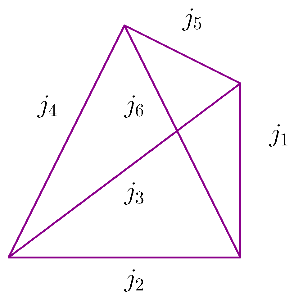
Table 1.
Probabilities for (k = 3) anyon excitations (a,a)in the ( = 2)-vacuum state.
| 0.599 | 0.383 | 0.017 | 0.001 |
Table 2.
Probabilities to find an (k = 3) anyon () for the fusion product of two plaquettes in the ( = 2)-vacuum state.
Table 2.
Probabilities to find an (k = 3) anyon () for the fusion product of two plaquettes in the ( = 2)-vacuum state.
| 0 | 1 | |||
|---|---|---|---|---|
| 0 | 0.524 | 0 | 0.0365 | 0 |
| 0 | 0.378 | 0 | 0.00261 | |
| 1 | 0.0365 | 0 | 0.0189 | 0 |
| 0 | 0.00261 | 0 | 0.000693 |
© 2018 by the author. Licensee MDPI, Basel, Switzerland. This article is an open access article distributed under the terms and conditions of the Creative Commons Attribution (CC BY) license (http://creativecommons.org/licenses/by/4.0/).
Share and Cite
MDPI and ACS Style
Dittrich, B. Cosmological Constant from Condensation of Defect Excitations. Universe 2018, 4, 81. https://0-doi-org.brum.beds.ac.uk/10.3390/universe4070081
AMA Style
Dittrich B. Cosmological Constant from Condensation of Defect Excitations. Universe. 2018; 4(7):81. https://0-doi-org.brum.beds.ac.uk/10.3390/universe4070081
Chicago/Turabian StyleDittrich, Bianca. 2018. "Cosmological Constant from Condensation of Defect Excitations" Universe 4, no. 7: 81. https://0-doi-org.brum.beds.ac.uk/10.3390/universe4070081
Note that from the first issue of 2016, this journal uses article numbers instead of page numbers. See further details here.