Strongly Intensive Observables in the Model with String Fusion †


Department of High Energy Physics and Elementary Particles, Saint Petersburg State University, 7/9 Universitetskaya nab., St. Petersburg 199034, Russia
*
Author to whom correspondence should be addressed.
†
This paper is based on the talk at the 7th International Conference on New Frontiers in Physics (ICNFP 2018), Crete, Greece, 4–12 July 2018.
‡
These authors contributed equally to this work.
Universe 2019, 5(1), 15; https://0-doi-org.brum.beds.ac.uk/10.3390/universe5010015
Submission received: 26 November 2018
/
Revised: 28 December 2018
/
Accepted: 29 December 2018
/
Published: 4 January 2019
(This article belongs to the Special Issue Selected Papers from the 7th International Conference on New Frontiers in Physics (ICNFP 2018))
Abstract
:We calculate the strongly intensive observables for multiplicities in two rapidity windows in the model with independent identical strings taking into account the charge sign of particles. We express the observables through the string pair correlation functions describing the correlations between the same and opposite sign particles produced in a string decay. We extract these charge-wise string two-particle correlation functions from the ALICE data on the forward-backward correlations and the balance function. Using them we predict the behavior of the charge-wise strongly intensive observables in the model with independent identical strings. We also show that the observable between multiplicities in two acceptance windows separated in rapidity, which is a strongly intensive in the case with independent identical strings, loses this property, when we take into account string fusion effects and a formation of strings of a few different types takes place in a collision. We predict the changes in the behaviour of this observable with energy and collision centrality, arising due to the string fusion phenomena.
1. Introduction
It is known that the investigations of long range rapidity correlations give the information about the initial stage of high energy hadronic interactions [1]. Therefore, to find a signature of the string fusion and percolation phenomenon [2,3,4] in ultrarelativistic heavy ion collisions the study of the correlations between multiplicities in two separated rapidity intervals, known as the forward-backward (FB) multiplicity correlations, was proposed [5].
Later it was realized [6,7,8,9] that the investigations of the FB correlations involving intensive observables in forward and backward observation windows, as e.g., the event-mean transverse momentum, enable to suppress the contribution of trivial “volume” fluctuations [10], originating from fluctuations in the number of initial sources (strings) and to obtain more clear signal on the process of string fusion, compared to usual FB multiplicity correlations.
In the present work, we explore another way to suppress the contribution of the “volume” fluctuations, passing to the more sophisticated correlation observable. In quark-gluon string model we calculate the strongly intensive variable
for the charged particles multiplicities and in forward and backward rapidity windows, introduced like in [11,12] to suppress the contribution of the "volume" fluctuations in hadronic interactions at high energy ( is a scaled variance).
We express this observable through the fundamental characteristics of a string: the multiplicity per unit of rapidity and the two-particle correlation function , describing the fragmentation of a single string (see Formula (6) below). We confirm the strongly intensive character of the observable in the case with fluctuating number of identical strings. It does not depend on the average number of strings, nor on the magnitude of event-by-event fluctuation of their number.
We also consider the strongly intensive observable (1) taking into account the particle charge sign. In the case of charge symmetry, which is a very good approximation for mid-rapidity region at LHC collision energies, these charge-wise strongly intensive observables are expressed through the string pair correlation functions for particles of the same and opposite signs, and . We get information about these two functions from the ALICE data on the FB correlations [13,14] and the balance function [15], using the relations (11) and (34). Finally, using these two-particle correlation functions of a string, we calculate the charge-wise strongly intensive observables , and .
We would like also to note that the variable , introduced by the Formula (1), is definitely not the only way to introduce the robust observable suppressing the trivial “volume” fluctuations. As an example, the application of the nonextensive statistical mechanics approach [16] to the multi-particle production was a great success. It allows a successful description of such subtle effects as particle rapidity distributions, an intermittence and fractal dimensions [17,18]. In particular this approach enables the description of particle transverse momentum distributions in the entire range of momenta, simultaneously in ’soft’ and ’hard’ regions, by the Tsallis-Pareto distribution [19]. However, the present paper considers only the multi-particle production in soft processes, which dominates in the total inelastic cross-section, and which can be described in the framework of a string model. We will also study the properties only of the strongly intensive observable defined by (1), leaving the remaining options for future research.
2. The Model with Independent Identical Strings
In this paper we restrict our consideration to a simple case of the model with independent identical strings [20]. In this model we suppose that the number of strings, N, fluctuates event by event around some mean value, , with some scaled variance, .
To characterize the properties of a single string we introduce the single and double distributions of particles produced from a single string fragmentation and the string two-particle correlation function defined by a standard way (see e.g., [21]):
In mid-rapidity region at LHC energies we assume the translation invariance in rapidity for the string characteristics. Then
For symmetric -azimuth rapidity observation windows and a symmetric reaction the definition of the strongly intensive variable (1) can be simplified to
where we imply that the observation windows and are separated by a rapidity gap , which corresponds to the distance between their centers. Clear that for symmetric reaction we have and
For small observation windows, of a width , where the is the characteristic correlation length for particles produced from the same string, we have shown in [14] that in the framework of the model with independent identical strings:
where is a distance between the centers of the forward an backward observation windows. Then by (4) we find
By (6) we really see that in the framework of this model the observable is a strongly intensive. It is independent of both the mean number of string and its fluctuation . It depends only on the string parameters , and the width of observation windows, . Whereas the scaled variance , (5), is an intensive, but not a strongly intensive observable, because although it is independent on the mean number of string , nevertheless through it depends on fluctuation of their number.
From the Formula (6) we see also the main properties of the , expecting in this model. Starting from the value 1 it increases with a distance between the centers of the observation windows, since the two-particle correlation function of a string decrease with . The extent of the increase with is proportional to the width of the observation windows . More detailed description of the needs the knowledge of the two-particle correlation function of a string .
3. The from Forward-Backward Correlations
In our paper [14] in the framework of the model with independent identical strings this function was fitted using the experimental pp ALICE data [13] on FB correlations between multiplicities in windows separated in rapidity and azimuth at three initial energies
together with the value of scaled variance of the number of strings . For the value of the parameters see Table 1 in that paper [14]. Recall that the comparison of the model with experimental data in [14] enables to fix only the product of the parameters , and . In (7) we imply that . For the periodic extension is implied.
4. with Charges
In Section 1 we have introduced the strongly intensive observable based on multiplicities of the all charged hadrons measured in two rapidity intervals. Now we consider various combinations of electric charges in these windows and similarly to Formula (1) we can define , , and . We can also introduce an additional strongly intensive observable that measures correlation between multiplicities of different charges in the same window and [22].
For symmetric reaction and symmetric windows ( invariance) we have , and the same for . In this case we have also , .
In case of additional charge symmetry ( invariance), we have , , , what is a very good approximation for mid-rapidity region at LHC collision energies. In this approximation we have for the distributions and two-particle correlation functions describing decay properties of a string:
where we also have taken into account the translation invariance, which takes place in mid-rapidity region at LHC energies. Easy to check that by definition (2)
For small observation windows in this approximation we find:
5. Connection with Balance Function
To obtain the correlation functions and separately we need some additional experimental information, as the FB correlations, used above, depend by (11) only on the sum of these two correlation functions. We use for this purpose else the recent results obtained by ALICE collaboration on the so-called balance function [15]. In this paper the balance function is defined to be proportional to the difference between unlike-sign and like-sign two-particle correlations functions:
where, for example, the correlation function in this paper is defined as follows
Here the is a “signal”, obtained from particle pair distribution. It is normalized by a mean number of a trigger (positive) particles. The is a “background”, obtained by the event mixing procedure. The coefficient is used to normalize the mixed-event distribution to unity in its maximum.
For a comparison with these experimental data we have to calculate the quantity , defined as in Formula (15) and (16), in the framework of our model. The can be expressed through the standard two-particle distribution (see e.g., Appendix C in [14]):
which is normalized as follows
For the in the background we have the same formula as (17), but with the replacement
The normalization conditions for one-particle distributions are as follows
The standard two-particle correlation function is defined as (see e.g., [21]):
If translation invariance in rapidity takes place, then we have the constant one-particle distributions:
and
(see Formula (18) in [14]). Then the standard two-particle correlation function is reduced to
In translation invariant case we can perform integration over and in (17). As a result we find:
where the is the phase space triangular weight function (see Appendix A in [14]):
Doing the integrations we implied that as indicated in Formula (17) , and hence . If we now, taking into account the -periodicity of the function , choose any fixed period , as a region of the variation, and reduce the other values of to this interval, then instead of (25) we get
where we have used that . We have used also here that .
Similarly for we find
The normalization constant for the background can be found from the condition that must be equal 1 in the maximum, where , what gives . Gathering we get
In last transition we took into account the charge symmetry, , which takes place in mid-rapidity region at LHC energies. Substituting this and the simular expressions for , and into (15) we get for the balance function
We have used that under charge symmetry and .
In paper [14] it was shown that in the model with independent identical strings the observed two-particle correlation function was expressed through the two-particle correlation function of a single string, as follows
Substituting them into (30) we find
where we have used that .
The rapidity projection of the can be found from the ALICE data [15], as a sum of the near- and away-side contributions:
which are defined in the ALICE paper, as follows
Taking into account our definition (8) of the , which corresponds the definition in paper [14] we get from (32)
It is important to take into account that the authors of the ALICE paper [15], defining by the di-hadron correlation method (16) the two-particle correlation functions, entering the definition of balance function (15), impose the requirement that the transverse momentum of the “trigger” particle must be higher than the “associated” one. This corresponds to the normalization by instead of in Formula (18). As a consequence we will have a factor instead of in Formula (34) for such normalization (see remark before the Section 6.1.1 in the paper [15]).
By (11) and (34) we can find the correlation functions and separately. For this we perform simultaneous fitting of the experimental data on pp collisions at 7 TeV for balance functions [15] and of extracted from FB correlations [13] (see Section 3). As the FB correlations were measured experimentally for minimum bias pp events, the results on balance functions for 70–80% pp centrality class were selected, assuming that the minimum bias is dominated by the peripheral collisions.
We use the simplest fit for the unlike-sign two-particle correlation function of a string:
For better data fitting of the like-sign two-particle correlation function we have to take into account else the HBT correlation term, important at small values of :
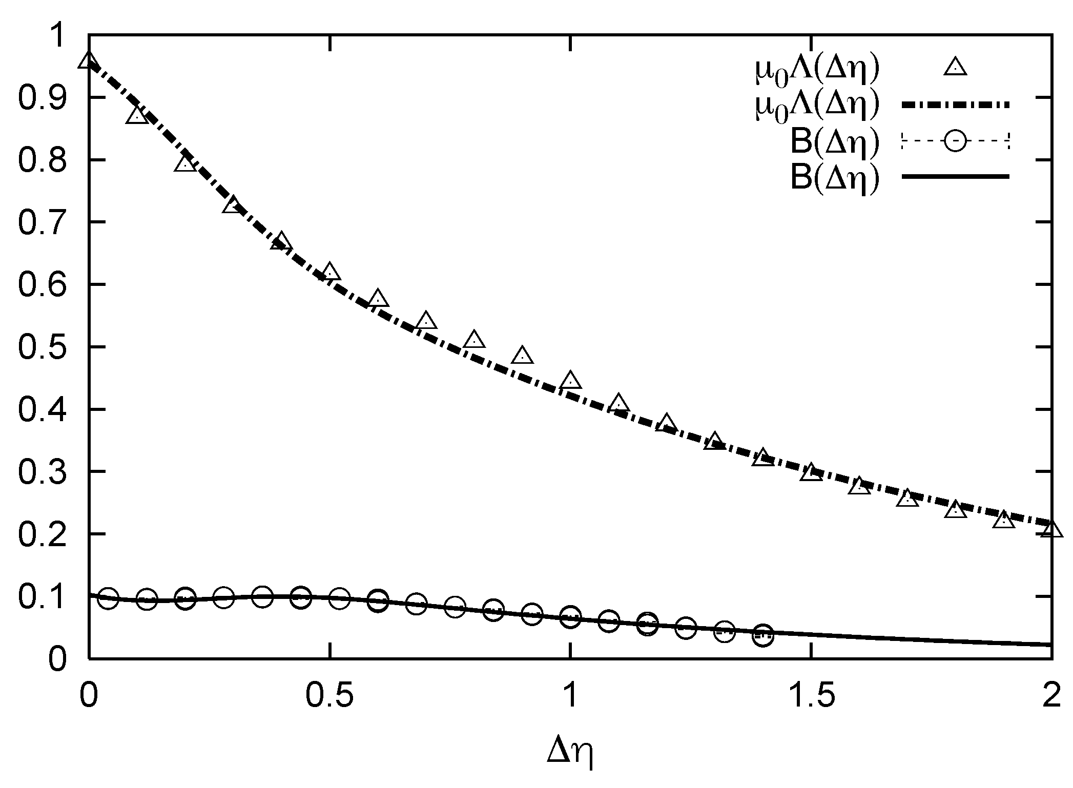
The results of the simultaneous fitting of the string two-particle correlation function , (11), extracted in [14] from the ALICE data [13] on FB correlations, and the balance function , (34), measured by ALICE [15] in pp collisions at 7 TeV are presented in Figure 1. This fitting fixes the parameters in Formulas (35) and (36) for the charge-wise correlation functions of a string: and , as presented in Table 1. We see that as expected the correlation length between opposite charge particles, , is smaller then the one between same charge particles, , due to local charge conservation in a string fragmentation process.
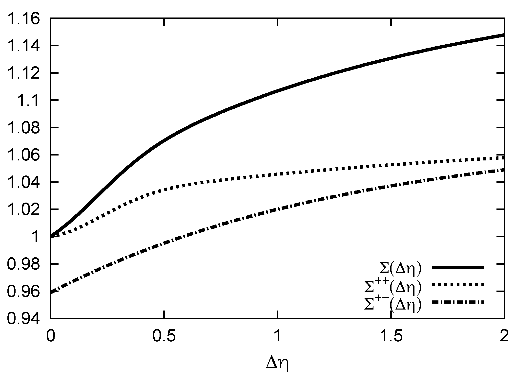
Now with the found charge-wise correlation functions of a string: and by Formulas (12) and (13) we can predict the behavior of the charge-wise strongly intensive observables , and in the model with independent identical strings. In Figure 2 these dependencies are presented for the case of two small observation windows as a function of rapidity gap between them. For comparison, the strongly intensive variable for the full multiplicities in these windows, given by the Formula (14), is also presented in this figure.
We see that as it was noted in the end of the Section 4 the = 0.96 ≠ 1 at , whereas the , like the total for full multiplicities.
6. String Fusion Effects
In this section we consider the influence of processes of interaction between strings on the strongly intensive observable . This influence increases with initial energy and with going from pp to heavy ion collisions. One of the possible ways to take these processes into account is to pass from the model with independent identical strings to the model with string fusion and percolation [2,3,4].
To account the string fusion processes we used approach with the finite lattice (the grid) in the impact parameter plane, suggested in [6] and later successfully exploited for a description of various phenomena (correlations, anisotropic azimuthal flows, the ridge) in ultra relativistic nuclear collisions. In this approach one splits the impact parameter plane into cells, which area is equal to the transverse area of single string and supposes the fusion of all strings with the centers in a given cell.
In this model the definite set of strings of different types corresponds to given event. Each such string, originating from a fusion of k primary strings, is characterized by its own parameters: the mean multiplicity per unit of rapidity, , and the string correlation function, . These parameters uniquely determine the strongly intensive observable, , between multiplicities, produced from decay of a string of a given kind k, defined by formulas similar to (1) and (4). For example, for small observation windows, , separated by the rapidity distance , similarly to (6), we have
In the model with k string types the direct calculation gives for the observable :
where is a mean number of particles produced from all sells with k fused strings in the rapidity observation window . Please note that the same result was obtained in the model with two types of strings in [12] for the long-range part of . Substituting (37) in Formula (38) we find
We see that in this case each string of the type k is characterized by two parameters: the product , where the is the mean multiplicity per unit of rapidity from a decay of such string, and its two-particle correlation length , which determines the correlations between particles, produced from a fragmentation of the string.
In the framework of the string fusion model [2,3,4] one usually supposes that the mean multiplicity per unit of rapidity for fused string, , increase as with k. The dependence of the correlation length on k is not so obvious. Basing on a simple geometrical picture of string fragmentation (see, e.g., [23,24,25,26]) one can expect the decrease of the correlation length, , with increase of k. In this picture with a growth of string tension the fragmentation process is finished at smaller string segments in rapidity. The correlation takes place only between particles originating from a fragmentation of neighbour string segments and hence the correlation length will decrease with k for fused strings.
Indirectly this fact is confirmed by the analysis [27] of the experimental STAR [28] and ALICE [29] data on net-charge fluctuations in pp and AA collisions. The dependence of net-charge fluctuations on the rapidity width of the observation window can be well described in a string model if one supposes the decrease of the correlation length with the transition to collisions of heavier nuclei and/or to higher energies, i.e., to collisions in which the proportion of fused strings is increasing.
By (41) both these factors, the increase of and the decrease of for fused string, lead to the steeper increase of , (37), with and to its saturation at a higher level . Due to (38) this behaviour transmits to the observable , as the last is a weighted average of with the weights , which are the mean portions of the particles produced from a given type of strings.
In real experiment we have always a mixture of fused and single strings. So with the transition to pp collisions at higher energy or/and to collisions of nuclei the proportion of fused strings will increase and we will observe the steeper increase of , with and its saturation at a higher level. Really, in Figure 3 we see such behaviour of , when we compare for pp collisions at three initial energies: 0.9, 2.76 and 7 TeV, calculated by using the two-particle correlation functions of a string , obtained by a fitting [14] of the experimental pp ALICE data [13] on FB correlations between multiplicities at these energies.
Table 2 illustrates the increase of and the decrease of the correlation length with energy for this data. Please note that these values are the some effective ones, because in the model at each energy we had supposed that all strings are identical. So they only indirectly reflects the influence of the increase of the proportion of fused strings with energy in pp collisions.
For studies of the dependence on multiplicity classes we can predict the behaviour similar to the one in Figure 3. For more central pp collisions due to the increase of the proportion of fused strings in such collisions we also have to observe the steeper increase of , with and its saturation at a higher level.
Please note that from a general point of view, this simultaneously means that the observable , strictly speaking, can not be considered any more as strongly intensive. Through the weight factors, , entering the Formula (38), the observable becomes dependent on collision conditions (e.g., on the collision centrality).
7. Conclusions
In the framework of the quark-gluon string model we have considered the observable for multiplicities and in two acceptance windows, and , separated by some rapidity interval , which usually used in the analysis of the multi-particle production in hadronic interactions at high energy, taking into account the charge sign of particles.
We express these observables through the fundamental string characteristics: the multiplicity per unit of rapidity and the string pair correlation functions describing the correlations between the same and opposite sign particles produced in a single string decay. We extract these charge-wise string two-particle correlation functions from the ALICE data on the FB correlations and the balance function. Using them we predict the behavior of the charge-wise strongly intensive observables in the model with independent identical strings.
We also discuss the influence of the process of string fusion on the string characteristics and on the behavior of the observables. We show that the observable , which is a strongly intensive in the case with independent identical strings, loses this property, when we take into account the string fusion processes and a formation of strings of a few different types takes place in a collision. In this situation the observable is proved to be equal to a weighted average of its values for different string types. Unfortunately, in this case through the weight factors this observable becomes dependent on collision conditions. We predict the changes in the behaviour of with energy and collision centrality, arising due to the string fusion phenomena.
Author Contributions
All authors contributed equally to this work.
Funding
The research was funded by the grant of the Russian Science Foundation (project 16-12-10176).
Conflicts of Interest
The authors declare no conflict of interest.
Abbreviations
The following abbreviations are used in this manuscript:
| FB | forward-backward |
| LHC | Large Hadron Collider |
References
- Dumitru, A.; Gelis, F.; McLerran, L.; Venugopalan, R. Glasma flux tubes and the near side ridge phenomenon at RHIC. Nucl. Phys. A 2008, 810, 91. [Google Scholar] [CrossRef]
- Biro, T.S.; Nielsen, H.B.; Knoll, J. Color Rope Model for Extreme Relativistic Heavy Ion Collisions. Nucl. Phys. B 1984, 245, 449. [Google Scholar] [CrossRef]
- Bialas, A.; Czyz, W. Conversion of Color Field Into Matter in the Central Region of High-energy Heavy Ion Collisions. Nucl. Phys. B 1986, 267, 242. [Google Scholar] [CrossRef]
- Braun, M.A.; Pajares, C. Particle production in nuclear collisions and string interactions. Phys. Lett. B 1992, 287, 154. [Google Scholar] [CrossRef]
- Amelin, N.S.; Armesto, N.; Braun, M.A.; Ferreiro, E.G.; Pajares, C. Long and short range correlations and the search of the quark gluon plasma. Phys. Rev. Lett. 1994, 73, 2813. [Google Scholar] [CrossRef] [PubMed]
- Braun, M.A.; Kolevatov, R.S.; Pajares, C.; Vechernin, V.V. Correlations between multiplicities and average transverse momentum in the percolating color strings approach. Eur. Phys. J. C 2004, 32, 535. [Google Scholar] [CrossRef]
- Alessandro, B.; Antinori, F.; Belikov, J.A.; Blume, C.; Dainese, A.; Foka, P.; Giubellino, P.; Hippolyte, B.; Kuhn, C. [ALICE Collaboration] ALICE: Physics Performance Report Volume II. J. Phys. G 2006, 32, 1295. [Google Scholar] [CrossRef]
- Vechernin, V.V.; Kolevatov, R.S. Long-range correlations between transverse momenta of charged particles produced in relativistic nucleus-nucleus collisions. Phys. Atom. Nucl. 2007, 70, 1809. [Google Scholar] [CrossRef]
- Kovalenko, V.; Vechernin, V. Forward-backward correlations between intensive observables. J. Phys. Conf. Ser. 2017, 798, 012053. [Google Scholar] [CrossRef] [Green Version]
- Bravina, L.V.; Bleibel, J.; Zabrodin, E.E. On the origin of forward–backward multiplicity correlations in pp collisions at ultrarelativistic energies. Phys. Lett. B 2018, 787, 146. [Google Scholar] [CrossRef]
- Gorenstein, M.I.; Gazdzicki, M. Strongly intensive quantities. Phys. Rev. C 2011, 84, 014904. [Google Scholar] [CrossRef]
- Andronov, E.V. Influence of the quark-gluon string fusion mechanism on long-range rapidity correlations and fluctuations. Theor. Math. Phys. 2015, 185, 1383. [Google Scholar] [CrossRef]
- Adam, J.; Adamova, D.; Aggarwal, M.M.; Aglieri Rinella, G.; Agnello, M.; Agrawal, N.; Ahammed, Z.; Ahmed, I.; Ahn, S.U.; Aimo, I.; et al. [ALICE Collaboration] Forward-backward multiplicity correlations in pp collisions at = 0.9, 2.76 and 7 TeV. JHEP 2015, 05, 097. [Google Scholar] [CrossRef]
- Vechernin, V. Forward–backward correlations between multiplicities in windows separated in azimuth and rapidity. Nucl. Phys. A 2015, 939, 21. [Google Scholar] [CrossRef]
- Adam, J.; Adamová, D.; Aggarwal, M.M.; Aglieri Rinella, G.; Agnello, M.; Agrawal, N.; Ahammed, Z.; Ahn, S.U.; Aiola, S.; Akindinov, A.; et al. [ALICE Collaboration] Multiplicity and transverse momentum evolution of charge-dependent correlations in pp, p–Pb, and Pb–Pb collisions at the LHC. Eur. Phys. J. C 2016, 76, 86. [Google Scholar] [CrossRef]
- Tsallis, C. Possible Generalization of Boltzmann-Gibbs Statistics. J. Stat. Phys. 1988, 52, 479. [Google Scholar] [CrossRef]
- Tsallis, C.; Brigatti, E. Nonextensive statistical mechanics: A brief introduction. Continuum Mech. Thermodyn. 2004, 16, 223. [Google Scholar] [CrossRef]
- Biro, T.S.; Purcsel, G.; Urmossy, K. Non-extensive approach to quark matter. Eur. Phys. J. A 2009, 40, 325. [Google Scholar] [CrossRef]
- Biro, T.S.; Urmossy, K.; Barnafoldi, G.G. Pion and Kaon Spectra from Distributed Mass Quark Matter. J. Phys. G 2008, 35, 044012. [Google Scholar] [CrossRef]
- Braun, M.A.; Pajares, C.; Vechernin, V.V. On the forward-backward correlations in a two stage scenario. Phys. Lett. B 2000, 493, 54. [Google Scholar] [CrossRef]
- Pruneau, C.; Gavin, S.; Voloshin, S. Methods for the study of particle production fluctuations. Phys. Rev. C 2002, 66, 044904. [Google Scholar] [CrossRef]
- Andronov, A. (for the NA61/SHINE Collab.) Energy dependence of fluctuations in p+p and Be+Be collisions from NA61/SHINE. J. Phys. Conf. Ser. 2016, 668, 012036. [Google Scholar] [CrossRef]
- Werner, K. Strings, pomerons, and the venus model of hadronic interactions at ultrarelativistic energies. Phys. Rep. 1993, 232, 87. [Google Scholar] [CrossRef]
- Artru, X. Classical String Phenomenology. 1. How Strings Work. Phys. Rep. 1983, 97, 147. [Google Scholar] [CrossRef]
- Vechernin, V.V. Space-Time Picture of String Fragmentation and the Fusion of Colour Strings. Relativistic Nuclear Physics and Quantum Chromodynamics. In Proceedings of the Baldin ISHEPP XIX, JINR, Dubna, v.1, Dubna, Russia, 29 September–4 October 2008; pp. 276–281. [Google Scholar]
- Bierlich, C.; Gustafson, G.; Lonnblad, L.; Tarasov, A. Effects of Overlapping Strings in pp Collisions. JHEP 2015, 03, 148. [Google Scholar] [CrossRef]
- Titov, A.; Vechernin, V. Net charge fluctuations in AA collisions in a simple string-inspired model. Proc. Sci. 2013, 173, 047. [Google Scholar] [CrossRef] [Green Version]
- Abelev, B.I.; Aggarwal, M.M.; Ahammed, Z.; Anderson, B.D.; Arkhipkin, D.; Averichev, G.S.; Bai, Y.; Balewski, J.; Barannikova, O.; Barnby, L.S.; et al. [STAR Collaboration] Beam-energy and system-size dependence of dynamical net charge fluctuations. Phys. Rev. C 2009, 79, 024906. [Google Scholar] [CrossRef]
- Abelev, B.I.; Adam, J.; Adamová, D.; Adare, A.M.; Aggarwal, M.M.; Aglieri Rinella, G.; Agocs, A.G.; Agostinelli, A.; Aguilar Salazar, S.; Ahammed, Z.; et al. [ALICE Collaboration] Net-Charge Fluctuations in Pb-Pb collisions at = 2.76 TeV. Phys. Rev. Lett. 2013, 110, 152301. [Google Scholar] [CrossRef]
Figure 1.
The results of simultaneous fitting (lines) by Formulas (11) and (34) of the string two-particle correlation function −, extracted in [14] from the ALICE data [13] on the FB correlations (see Section 3), and the balance function - ∘, measured by ALICE [15] in pp collisions at 7 TeV.

Figure 2.
The charge-wise strongly intensive variables: (dotted line) and (dash-dotted line) with two small observation windows as a function of rapidity gap between them, calculated by formulas (12–13) with the string correlation functions and obtained by the fit procedure shown in Figure 1. Full line—the strongly intensive observable for the full multiplicities in these windows, given by the Formula (14).

Figure 3.
The strongly intensive observable, , between multiplicities in two small pseudorapidity windows (of the width 0.2 and 0.4) as a function of the distance between window centers, at three initial energies: 0.9, 2.76 and 7 TeV.
Figure 3.
The strongly intensive observable, , between multiplicities in two small pseudorapidity windows (of the width 0.2 and 0.4) as a function of the distance between window centers, at three initial energies: 0.9, 2.76 and 7 TeV.


Table 1.
The value of the parameters in Formulas (35) and (36) for the charge-wise correlation functions of a string: and , obtained by the fit procedure, presented in Figure 1.
| a | |||
|---|---|---|---|
| 1.16 | 0.5 | 0.25 | |
| 1.34 | 1.87 | 0.33 |
Table 2.
The value of the parameters in the exponetial approximations of the type (40) for the two-particle correlation function of a string , obtained by a fitting [14] of the experimental pp ALICE data [13] on FB correlations between multiplicities at three initial energies.
| , TeV | 0.9 | 2.76 | 7.0 |
|---|---|---|---|
| 0.73 | 0.83 | 0.93 | |
| 1.52 | 1.43 | 1.33 |
© 2019 by the authors. Licensee MDPI, Basel, Switzerland. This article is an open access article distributed under the terms and conditions of the Creative Commons Attribution (CC BY) license (http://creativecommons.org/licenses/by/4.0/).
Share and Cite
MDPI and ACS Style
Vechernin, V.; Andronov, E. Strongly Intensive Observables in the Model with String Fusion. Universe 2019, 5, 15. https://0-doi-org.brum.beds.ac.uk/10.3390/universe5010015
AMA Style
Vechernin V, Andronov E. Strongly Intensive Observables in the Model with String Fusion. Universe. 2019; 5(1):15. https://0-doi-org.brum.beds.ac.uk/10.3390/universe5010015
Chicago/Turabian StyleVechernin, Vladimir, and Evgeny Andronov. 2019. "Strongly Intensive Observables in the Model with String Fusion" Universe 5, no. 1: 15. https://0-doi-org.brum.beds.ac.uk/10.3390/universe5010015
Note that from the first issue of 2016, this journal uses article numbers instead of page numbers. See further details here.