QUBIC: Exploring the Primordial Universe with the Q&U Bolometric Interferometer †

 , , , , , , , , , , ,
  , , , ,
Abstract
:1. Introduction
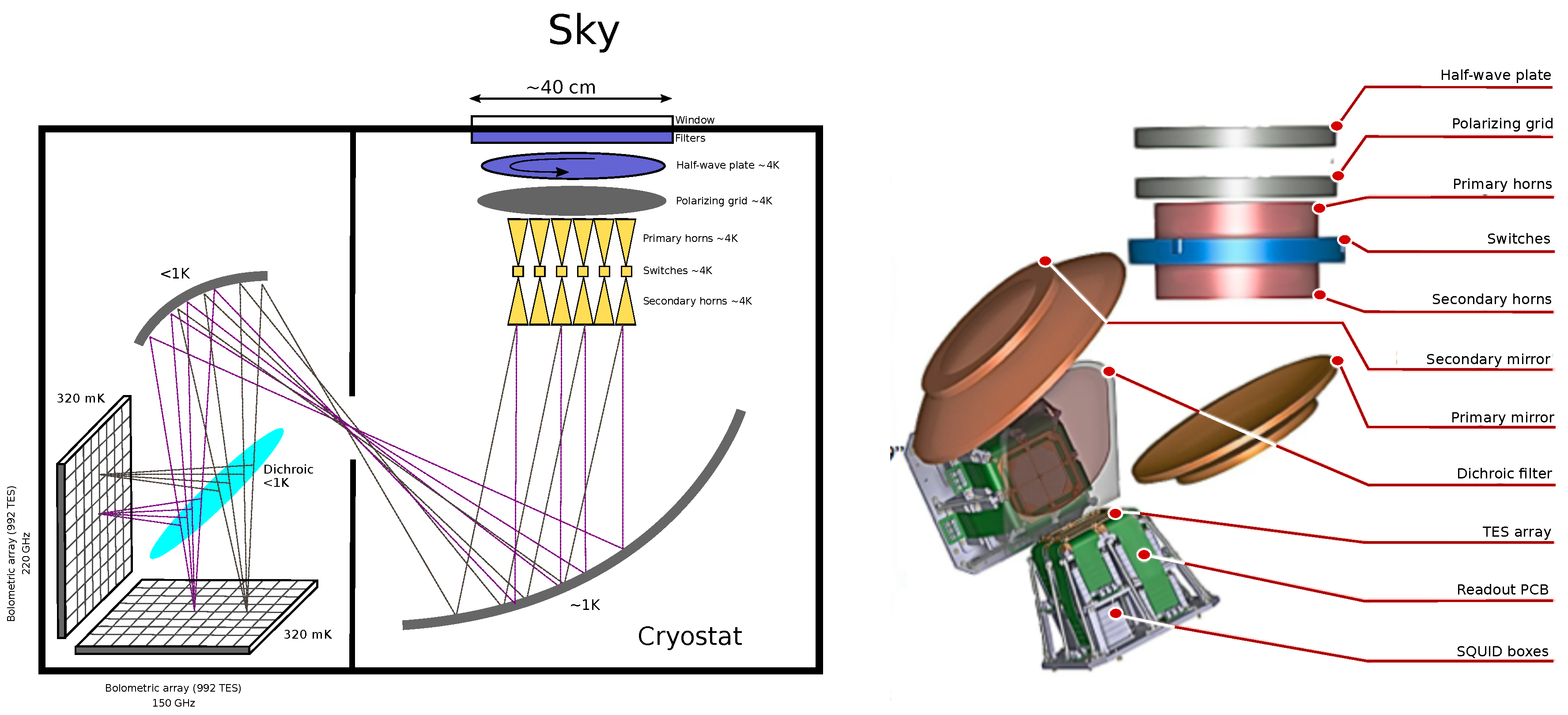
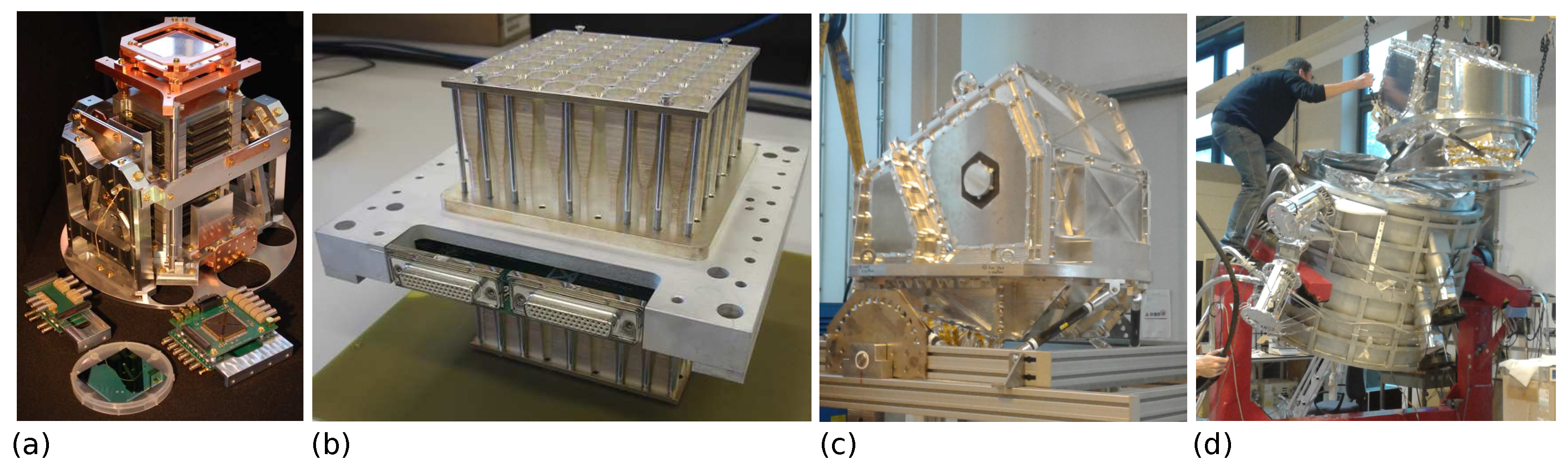
2. The Instrument
3. Measurement, Self-Calibration, and Spectral Imaging
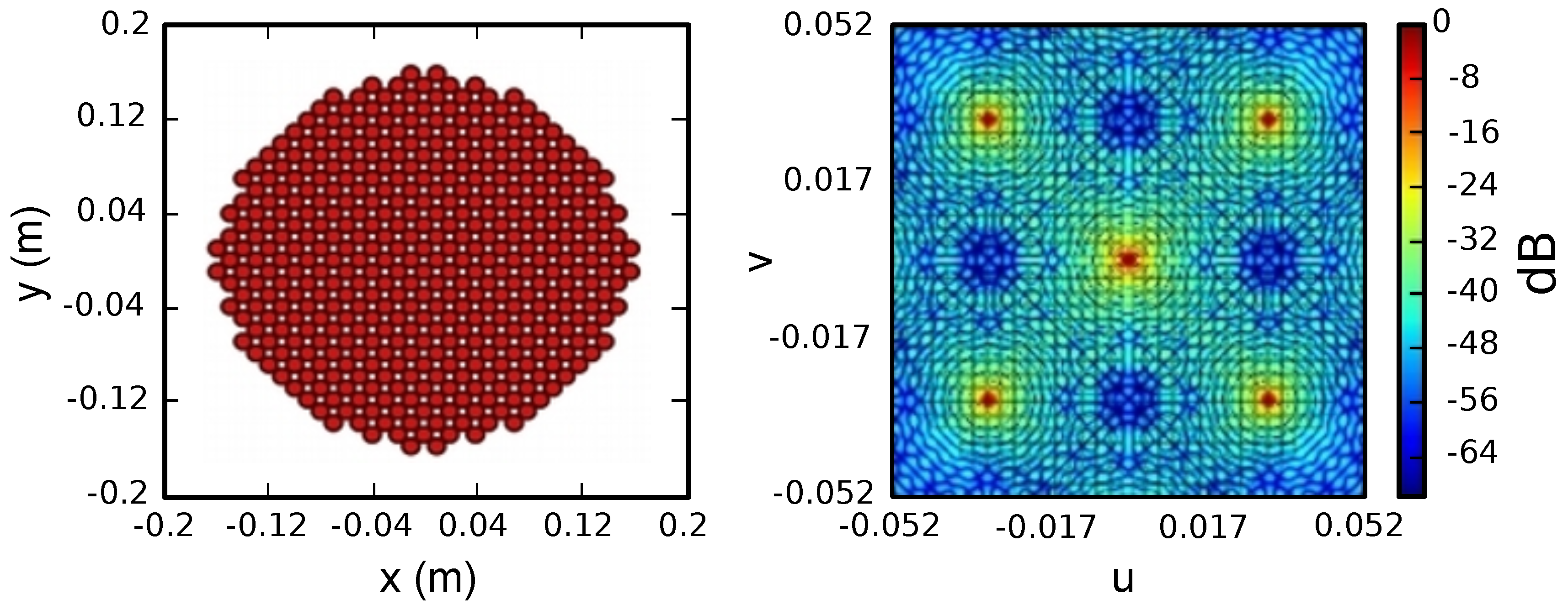
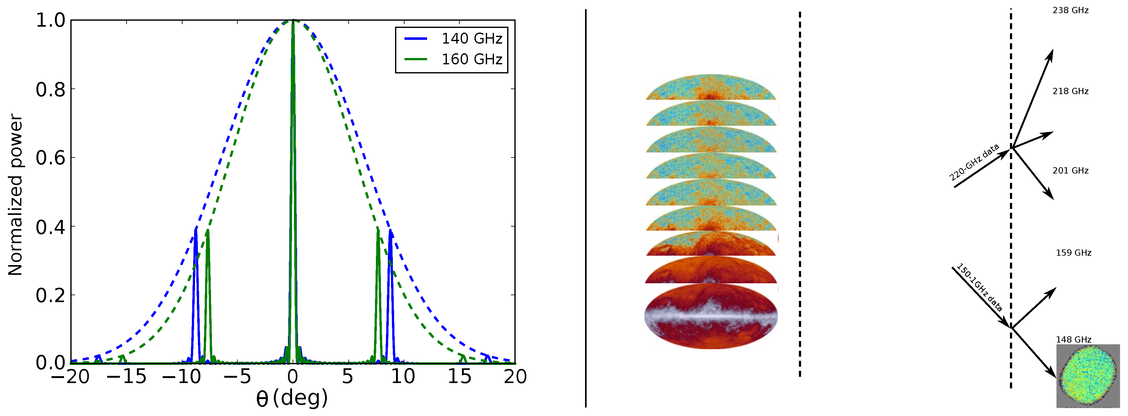
3.1. Signal Model and Synthetic Beam
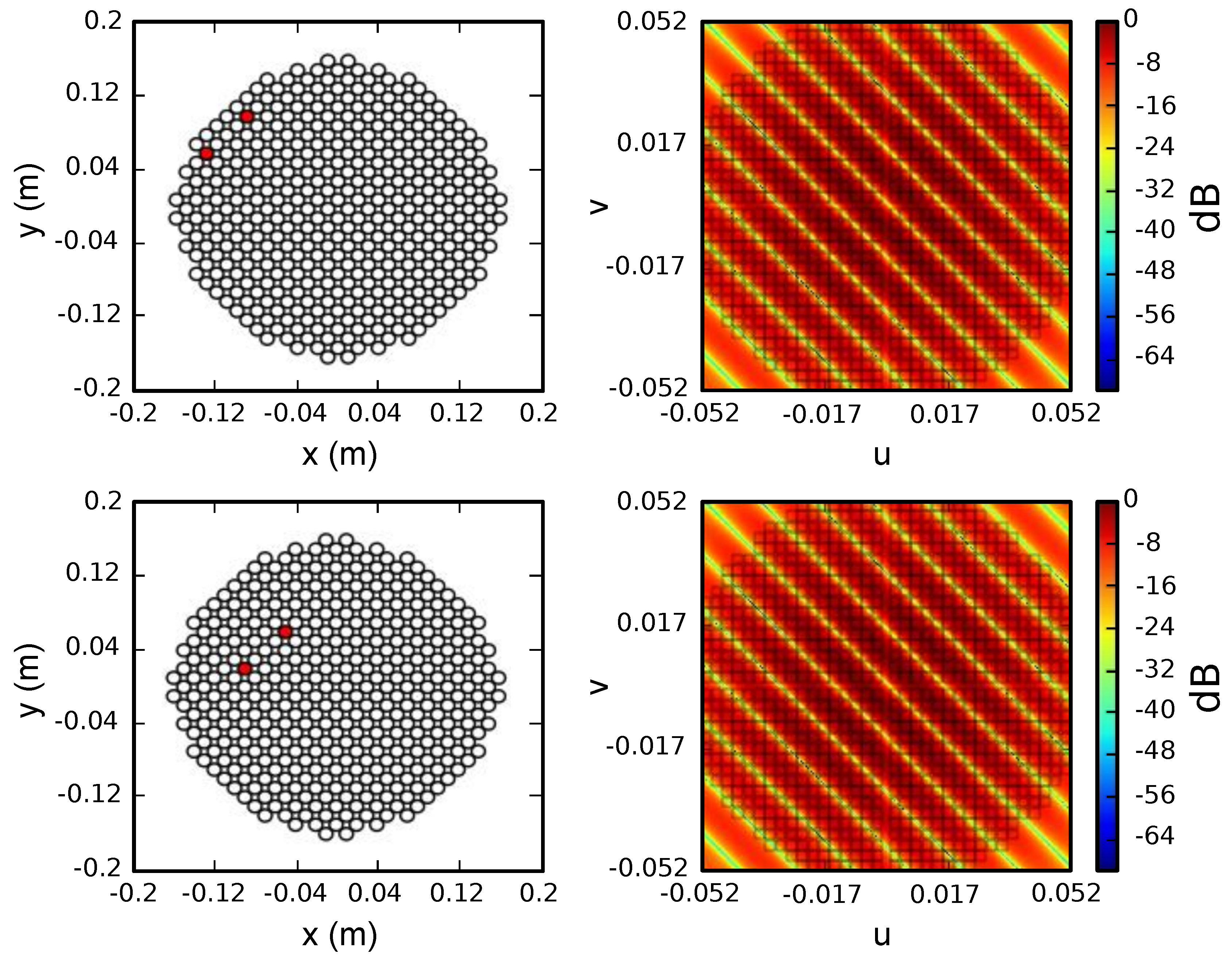
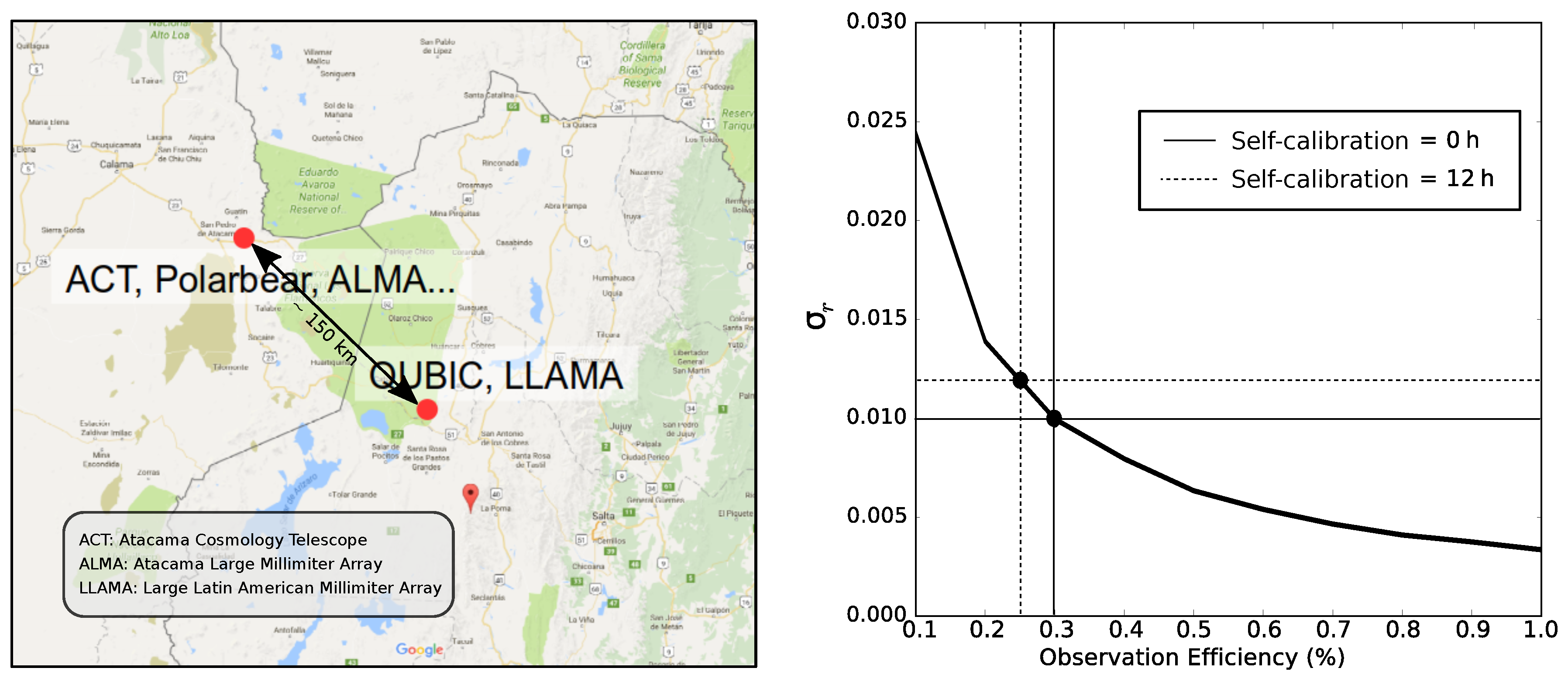
3.2. Self-Calibration
3.3. Spectral Imaging
4. The QUBIC Site
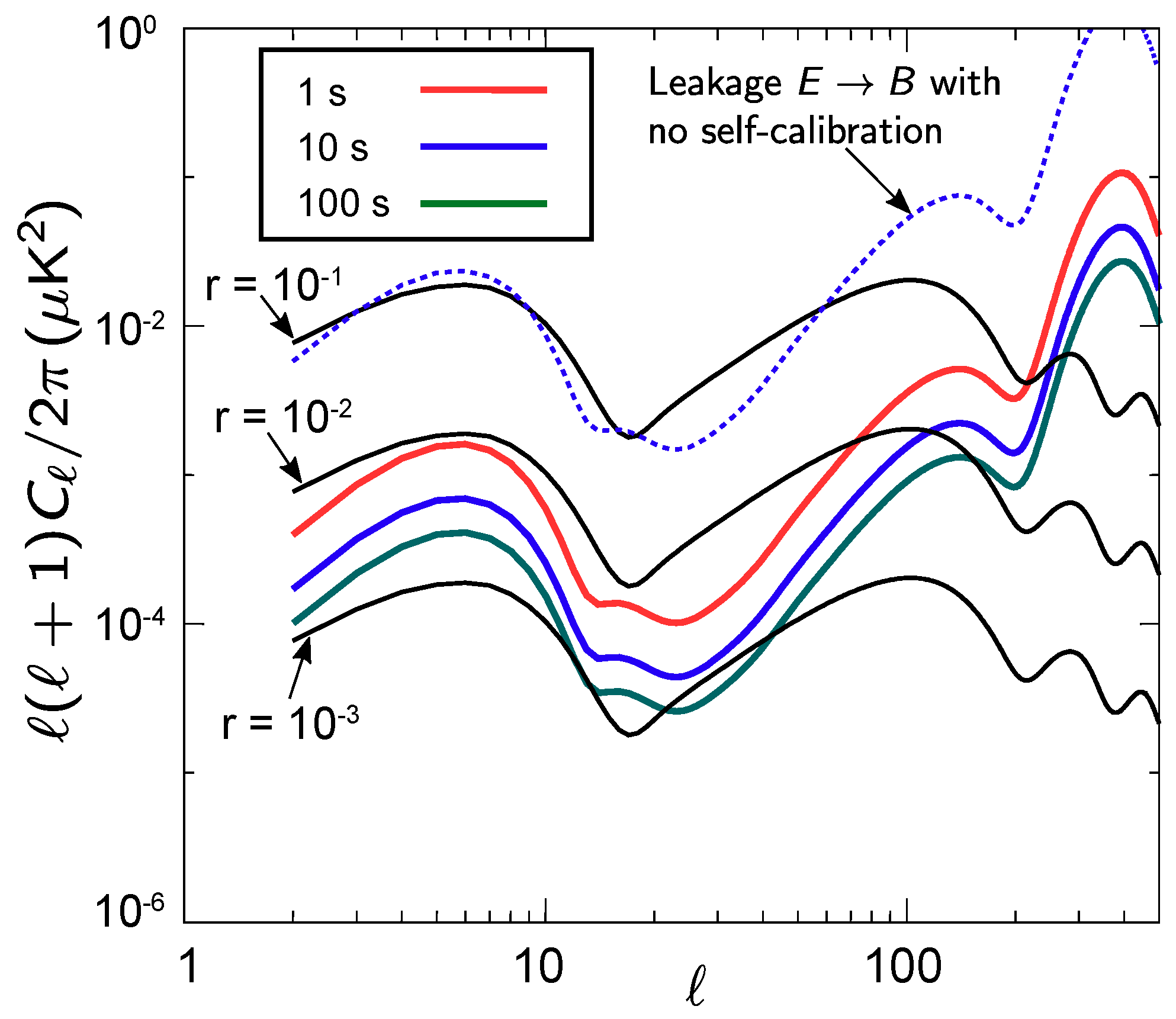
5. Scientific Performance
6. Current Status
7. Conclusions
Funding
Conflicts of Interest
References
- Battistelli, E.; Baú, A.; Bennett, D.; Bergé, L.; Bernard, J.P.; de Bernardis, P.; Bounab, A.; Bréelle, É.; Bunn, E.F.; Calvo, M.; et al. QUBIC: The QU bolometric interferometer for cosmology. Astropart. Phys. 2011, 34, 705–716. [Google Scholar] [CrossRef]
- Tartari, A.; Aumont, J.; Banfi, S.; Battaglia, P.; Battistelli, E.S.; Baù, A.; Bélier, B.; Bennett, D.; Bergé, L.; Bernard, J.P.; et al. QUBIC: A Fizeau Interferometer Targeting Primordial B-Modes. J. Low Temp. Phys. 2015, 181. [Google Scholar] [CrossRef]
- Aumont, J.; Banfi, S.; Battaglia, P.; Battistelli, E.S.; Baù, A.; Bélier, B.; Bennett, D.; Bergé, L.; Bernard, J.P.; Bersanelli, M.; et al. QUBIC Technical Design Report. arXiv, 2016; arXiv:1609.04372. [Google Scholar]
- Liu, A.; Tegmark, M.; Morrison, S.; Lutomirski, A.; Zaldarriaga, M. Precision calibration of radio interferometers using redundant baselines. Mon. Not. R. Astron. Soc. 2010, 408, 1029–1050. [Google Scholar] [CrossRef]
- Bigot-Sazy, M.A.; Charlassier, R.; Hamilton, J.; Kaplan, J.; Zahariade, G. Self-calibration: An efficient method to control systematic effects in bolometric interferometry. Astron. Astrophys. 2013, 550, A59. [Google Scholar] [CrossRef]
- De Bernardis, P.; Ade, P.; Amico, G.; Auguste, D.; Aumont, J.; Banfi, S.; Barbarán, G.; Battaglia, P.; Battistelli, E.; Baù, A.; et al. QUBIC: Measuring CMB polarization from Argentina. Bol. Asoc. Argent. Astron. Plata Argent. 2018, 60, 107–114. [Google Scholar]
- Errard, J.; Feeney, S.M.; Peiris, H.V.; Jaffe, A.H. Robust forecasts on fundamental physics from the foreground-obscured, gravitationally-lensed CMB polarization. J. Cosmol. Astropart. Phys. 2016, 2016, 052. [Google Scholar] [CrossRef]
- Hui, H.; Ade, P.A.R.; Ahmed, Z.; Alexander, K.D.; Amiri, M.; Barkats, D.; Benton, S.J.; Bischoff, C.A.; Bock, J.J.; Boenish, H.; et al. BICEP3 focal plane design and detector performance. In Proceedings of the SPIE Proceedings for Millimeter, Submillimeter, and Far-Infrared Detectors and Instrumentation for Astronomy VIII, Edinburgh, UK, 28 June–1 July 2016; Volume 9914, p. 99140T-1. [Google Scholar] [CrossRef]
- Harrington, K.; Marriage, T.; Ali, A.; Appel, J.W.; Bennett, C.L.; Boone, F.; Brewer, M.; Chan, M.; Chuss, D.T.; Colazo, F.; et al. The Cosmology Large Angular Scale Surveyor. In Proceedings of the Millimeter, Submillimeter, and Far-Infrared Detectors and Instrumentation for Astronomy VIII, Edinburgh, UK, 28 June–1 July 2016; Volume 9914, p. 99141K-1. [Google Scholar] [CrossRef]
- Benson, B.A.; Ade, P.A.R.; Ahmed, Z.; Allen, S.W.; Arnold, K.; Austermann, J.E.; Bender, A.N.; Bleem, L.E.; Carlstrom, J.E.; Chang, C.L.; et al. SPT-3G: A next-generation cosmic microwave background polarization experiment on the South Pole telescope. In Proceedings of the Millimeter, Submillimeter, and Far-Infrared Detectors and Instrumentation for Astronomy VII, Montreal, QC, Canada, 22–27 June 2014; Volume 9153, p. 91531P. [Google Scholar] [CrossRef]
- Li, Y.; Austermann, J.E.; Beall, J.A.; Bruno, S.M.; Choi, S.K.; Cothard, N.F.; Crowley, K.T.; Duff, S.M.; Gallardo, P.A.; Henderson, S.W.; et al. Performance of the advanced ACTPol low frequency array. In Proceedings of the Millimeter, Submillimeter, and Far-Infrared Detectors and Instrumentation for Astronomy IX, Austin, TX, USA, 10–15 June 2018; Volume 10708, p. 107080A. [Google Scholar] [CrossRef]
- Keating, B. The POLARBEAR and Simons Array CMB Polarization Experiments. J. Low Temp. Phys. 2016, 184, 805–810. [Google Scholar] [CrossRef]


| Project | Frequencies (GHz) | ℓ Range | Ref. | Goal | |
|---|---|---|---|---|---|
| no fg. | with fg. | ||||
| QUBIC | 150, 220 | 30–200 | |||
| Bicep3/Keck | 95, 150, 220 | 50–250 | [8] | ||
| CLASS | 38, 93, 148, 217 | 2–100 | [9] | ||
| SPT-3G | 95, 148, 223 | 50–3000 | [10] | ||
| AdvACT | 90, 150, 230 | 60–3000 | [11] | ||
| Simons Array | 90, 150, 220 | 30–3000 | [12] | ||
© 2019 by the authors. Licensee MDPI, Basel, Switzerland. This article is an open access article distributed under the terms and conditions of the Creative Commons Attribution (CC BY) license (http://creativecommons.org/licenses/by/4.0/).
Share and Cite
Mennella, A.; Ade, P.; Amico, G.; Auguste, D.; Aumont, J.; Banfi, S.; Barbaràn, G.; Battaglia, P.; Battistelli, E.; Baù, A.; et al. QUBIC: Exploring the Primordial Universe with the Q&U Bolometric Interferometer. Universe 2019, 5, 42. https://0-doi-org.brum.beds.ac.uk/10.3390/universe5020042
Mennella A, Ade P, Amico G, Auguste D, Aumont J, Banfi S, Barbaràn G, Battaglia P, Battistelli E, Baù A, et al. QUBIC: Exploring the Primordial Universe with the Q&U Bolometric Interferometer. Universe. 2019; 5(2):42. https://0-doi-org.brum.beds.ac.uk/10.3390/universe5020042
Chicago/Turabian StyleMennella, Aniello, Peter Ade, Giorgio Amico, Didier Auguste, Jonathan Aumont, Stefano Banfi, Gustavo Barbaràn, Paola Battaglia, Elia Battistelli, Alessandro Baù, and et al. 2019. "QUBIC: Exploring the Primordial Universe with the Q&U Bolometric Interferometer" Universe 5, no. 2: 42. https://0-doi-org.brum.beds.ac.uk/10.3390/universe5020042