Two Types of Jets and Quark and Chromon Model in QCD †

1
School of Physics and Astronomy, Seoul National University, Seoul 08826, Korea
2
Center for Quantum Spacetime, Sogang University, Seoul 04107, Korea
†
This paper is based on the talk at the 7th International Conference on New Frontiers in Physics (ICNFP 2018), Crete, Greece, 4–12 July 2018.
Universe 2019, 5(2), 62; https://0-doi-org.brum.beds.ac.uk/10.3390/universe5020062
Submission received: 8 January 2019
/
Revised: 31 January 2019
/
Accepted: 11 February 2019
/
Published: 14 February 2019
(This article belongs to the Special Issue Selected Papers from the 7th International Conference on New Frontiers in Physics (ICNFP 2018))
Abstract
:We discuss the importance of the color reflection symmetry of the Abelian decomposition in QCD. The Abelian decomposition breaks up the color gauge field to three parts, the neuron, chromon, and the topological monopole, gauge independently. Moreover, it refines the Feynman diagram in such a way that the conservation of color is explicit. This leads us to generalize the quark model to the quark and chromon model. We show how the Abelian decomposition reduces the non-Abelian color gauge symmetry to the simple discrete 24 element color reflection symmetry which assumes the role of the color gauge symmetry and plays the central role in the quark and chromon model.
Keywords:
Abelian decomposition; decomposition of Feynman diagram in QCD; quark and chromon model; color reflection group; color reflection invariance; glueball spectrum; glueball-quarkonium mixingPACS:
12.38.-t; 12.38.Aw; 11.15.-q; 11.15.Tk1. Introduction
One of the widely held misunderstandings in gauge theory is that the non-Abelian gauge symmetry is so tight that it defines the theory almost uniquely, and thus does not allow any simplification. The Abelian decomposition of QCD tells that this popular wisdom is not true [1,2,3,4]. It shows that QCD has a non-trivial core, the restricted QCD (RCD), which describes the Abelian sub-dynamics of QCD but has the full non-Abelian gauge symmetry. Moreover, we can separate it from QCD gauge independently.
Before we discuss the Abelian decomposition, it is important to understand why we need this. Consider the proton, which is made of three valence quarks. However, obviously we need the gluons to bind the quarks in the proton. However, the quark model tells that the proton has no valence gluon. If so, what is the binding gluon which bind the quarks in proton, and how do we distinguish it from the valence gluon? To answer this we need the Abelian decomposition.
Another motivation for the Abelian decomposition is to understand the color confinement problem in QCD. Two popular approaches proposed to resolve this problem are the monopole condensation and the Abelian dominance. Nambu and Mandelstam proposed that the monopole condensation could generate the dual Meissner effect and confine the color in QCD [5,6,7]. On the other hand ’tHooft proposed that the Abelian part of gluons could be responsible for the color confinement in QCD [8]. To prove the monopole condensation, however, we first have to separate out the monopole part from the QCD gauge potential gauge independently. Similarly, to prove the Abelian dominance we have to know what is the Abelian part and how to separate it. To do this we need the Abelian decomposition.
The Abelian decomposition breaks up the non-Abelian gauge potential to two different parts, the color neutral restricted (Abelian) part which has the full non-Abelian gauge symmetry and describes the Abelian sub-dynamics of QCD, and the gauge covariant valence (non-Abelian) part which describes the colored gluons (the chromons) and plays the role of the colored source of QCD, gauge independently [1,2,3,4]. Moreover, it separates the restricted part to the non-topological Maxwell part which describes the genuine Abelian potential which represents the color neutral binding gluons (the neurons) and topological Dirac part which describes the non-Abelian monopole potential gauge independently [1,2,3,4].
The Abelian decomposition has deep physical consequences. First of all, it shows that there is a simpler QCD called RCD made of the restricted potential, which describes the Abelian sub-dynamics of QCD. Moreover, it tells that QCD can be viewed as RCD which has the chromons as the colored source. So we can tell exactly what is the Abelian part of QCD without ambiguity, and separate it gauge independently.
This allows us to prove the Abelian dominance; that indeed RCD (i.e., the Abelian part of QCD) is responsible for the confinement [8,9]. Since the non-Abelian part describes the colored chromons which have to be confined, it cannot play any role in the confinement. This is because the confined prisoner cannot be the confining agent. So only the Abelian part of the gluons must be responsible for the confinement.
This can be proved rigorously. Theoretically it can be shown that only the restricted potential contributes to the Wilson loop integral that generates the confining force [9]. Moreover, we can demonstrate this numerically in lattice QCD [10,11,12,13,14,15]. Actually we can establish not just the Abelian dominance but the monopole dominance, which tells that the monopole part of the restricted potential is responsible for the confinement. Implementing the Abelian decomposition on lattice, we can calculate the Wilson loop integral with the full potential, the restricted potential, and the monopole potential separately, and show that all three potentials give us exactly the same linear confining force. This explicates the monopole dominance, that the monopole potential is enough to generate the confining force.
The monopole dominance is not incompatible with the Abelian dominance, because the monopole is a part of the restricted potential. Indeed the monopole dominance assures the Abelian dominance. However, it does not tell how the monopole confines the color. To tell how, we have to prove the monopole condensation. The Abelian decomposition allows us to do that.
Savvidy first tried to prove the monopole condensation, and has almost succeeded [16]. He obtained the magnetic condensation known as the Savvidy vacuum. Unfortunately, it was unstable. Worse, it was not gauge invariant. Many people tried to remove these defects unsuccessfully [17,18,19,20,21,22,23,24,25]. There are two critical defects in these calculations. They could not separate the monopole part gauge independently, and could not implement the gauge invariance properly in the calculations [26,27,28,29].
The Abelian decomposition can solve these problems and demonstrate the monopole condensation gauge independently. It separates the monopole part gauge independently and puts QCD to the background field formalism. So, choosing the monopole potential as the background and integrating out the chromons gauge invariantly, we can calculate the QCD effective potential and prove that the true QCD vacuum is given by the gauge invariant monopole condensation [30,31].
As importantly, the Abelian decomposition explains that there are actually two different types of gluons in QCD which play totally different roles, the color neutral neurons which provide the binding of the colored source and the colored chromons which become the constituent of hadrons [1,2,3,4]. This plays an important role in hadron spectroscopy. This is because the chromons (just like the quarks) become the constituent of hadrons, while the neurons play the role of the binding gluons. This generalizes the quark model to the quark and chromon model. In particular, this plays the essential role for us to understand the glueball spectrum and its mixing with quarkonium [32,33,34].
This neatly answers the question on the binding gluon and the valence gluon in the proton. Clearly the binding gluons in the proton are the neurons, and the proton has no colored chromons as the valence gluon which can change the position of the proton in the hadron spectroscopy.
Moreover, with two types of gluons we can refine and decompose the gluon propagators in the Feynman diagram to the neuron and chromon propagators in such a way that the color conservation is explicit. This sheds a new light to the QCD Feynman diagrams, and makes a deep impact on the perturbative QCD [30,31,32,33,34].
The Abelian decomposition raises a fundamental question. In the conventional QCD where all gluons are treated equally, the gluons form an SU(3) octet. However, the Abelian decomposition tells that there are two types of gluons which play different roles. If so, what is the symmetry which describes the neurons and chromons? Is the SU(3) symmetry still valid, and do they still form an octet? If not, how are they classified?
To answer these questions, we have to understand that after the Abelian decomposition the non-Abelian SU(3) symmetry is reduced to a simple discrete symmetry called the color reflection symmetry [1,2,3,4]. This means that after the Abelian decomposition the color reflection symmetry replaces the complicated SU(3) color gauge symmetry, so that the color reflection invariance guarantees the color gauge invariance. This greatly simplifies us to implement gauge invariance in the calculation of the QCD effective potential [30,31].
Furthermore, this symmetry plays the fundamental role in the hadron spectroscopy in the quark and chromon model [32,33,34]. To understand how the color reflection symmetry works, we must know how the neurons and chromons transform under the color reflection. The purpose of this paper is to discuss the origin of the color reflection symmetry and study how it affects the hadron spectroscopy.
The paper is organized as follows. In Section 2 we review the Abelian decomposition of QCD for later purpose. In Section 3 we discuss how the color reflection symmetry originates after the Abelian decomposition and how the neurons and chromons transform under the color reflection. In Section 4 we discuss how the color reflection invariance allows us to demonstrate the monopole condensation gauge independently. In Section 5 we discuss how the fundamental feature of the Abelian decomposition, the existence of two types of gluons, can be tested experimentally at LHC. In the last section we discuss the physical implications of our result.
2. Abelian Decomposition of QCD: A Review
To obtain the Abelian decomposition of SU(3) QCD we have to understand the Abelian decomposition of SU(2) QCD first, because it plays an essential role in the SU(3) QCD. So we start from the SU(2) QCD.
Let be an arbitrary right-handed local orthonormal basis of SU(2) QCD. To make the Abelian decomposition we choose any direction, for example , to be the Abelian direction and impose the isometry condition to project out the restricted potential [1,2,3,4]
This is the Abelian projection which projects out the restricted (i.e., Abelian) potential .
It has the following properites. First, it is the potential which leaves the Abelian direction invariant (which makes the Abelian direction covariantly constant) under the parallel transport. Second, it is made of two parts, the non-topological (Maxwellian) which describes the color neutral Abelian gluon (the neuron) and the topological (Diracian) which describes the non-Abelian monopole [35,36]. Most importantly, the projection is gauge independent, because is arbitrary.
With this we have
Please note that although and are Abelian, they are made of two potentials, the non-topological and topological . This dual structure shows that there are actually two possible magnetic background to choose, the Savvidy background coming from and the monopole background coming from , in the calculation of the QCD effective action [26,27,28,29].
With (2) we can construct the restricted QCD (RCD) which has the full non-Abelian gauge symmetry yet much simpler than QCD,
which describes the Abelian sub-dynamics of QCD.
With the Abelian projection we can express the full SU(2) potential adding the non-Abelian part to [1,2,3,4]
With this we can show that has the full gauge degrees of freedom, while transforms gauge covariantly
This is because the connection space forms an Affine space. So can be viewed to describe the colored gluon (the chromon) which becomes the gauge covariant source. This is the Abelian decomposition. Moreover, with
we obtain the extended QCD (ECD)
to recover the full QCD. This shows that QCD can be viewed as RCD which has the chromon as the colored source [1,2,3,4].
An important advantage of the Abelian decomposition is that it can actually “abelianize” the non-Abelian gauge theory gauge independently [1,2,3,4]. To see this notice that with
we have
So, expressing the chromon by the complex vector , we can put the Lagrangian explicitly in the Abelian form,
One might wonder how the non-Abelian structure disappears in this Abelianization. Actually the non-Abelian structure is not disappeared but hidden. To see this, first notice that the Abelian formalism is expressed by the dual potential given by the sum of two potentials and . Clearly represents the topological degrees of the non-Abelian symmetry which does not exist in the naive Abelianization that one obtains by fixing the gauge [1,2,3,4].
To see how the non-Abelian gauge symmetry is realized in this Abelian formalism, let
Certainly the Lagrangian (9) is invariant not only under the active (classical) gauge transformation (5) given by
but also under the following passive (quantum) gauge transformation
This tells that the Abelian theory not only retains the original (classical) gauge symmetry, but actually has an enlarged (quantum) gauge symmetry. It is this quantum gauge symmetry which keeps the chromon massless.
The reason for this extra (quantum) gauge symmetry is that the Abelian decomposition automatically put the theory in the background field formalism which doubles the gauge symmetry [37,38]. This is because in this decomposition we can view the restricted and valence parts and (or equivalently and in the non-Abelian formalism) as the classical and quantum parts, so that we have freedom to assign the gauge symmetry to both classical and quantum field.
Mathematically ECD is identical to QCD, but physically it provides a totally new meaning to QCD. It tells that QCD has two types of gluons, the neuron and chromon, which plays different roles. The neuron, together with the topological monopole potential, provides the binding. On the other hand the chromon, just like the quarks, becomes the colored constituent of hadrons which has to be confined [30,31,32,33,34].
The Abelian decomposition of SU(3) QCD is more complicated but straightforward [30,31]. Since SU(3) has rank two, it has two Abelian directions. Let be the orthonormal SU(3) basis, and choose and to be the Abelian directions. To make the Abelian projection, we impose the isometry
This automatically guarantees [35]
where ∗ denotes the d-product. This tells that we actually need one -like Abeiian direction to make the Abelian decomposition, although SU(3) has two Abelian directions.
Solving (13), we have the SU(3) Abelian projection,
where and are two SU(3) neurons, and the sum is the sum of the three Abelian directions of three SU(2) subgroups made of , , and . Please note that although SU(3) has two Abelian directions, is expressed by three SU(2) in a Weyl symmetric way. The Weyl group of SU(N) is the permutation group of N colors of SU(N), which is mathematically the symmetric group of order N.
Clearly the three SU(2) neurons are not linearly independent, because they are expressed by two neurons and . However, the Weyl symmetric expression plays a very important role because it allows us to calculate the SU(3) QCD effective action in terms of the SU(2) QCD effective action [30,31].
From (15) we have the SU(3) RCD
which has the full SU(3) gauge symmetry. Again notice that it can be expressed in a Weyl symmetric way.
With the Abelian projection we have the Abelian decomposition of the SU(3) gauge potential,
Here again transforms covariantly. Moreover, it can be decomposed to the three chromons of SU(2) subgroups , which can be identified as the red, blue, and green chromons . From this we have
With this we obtain the SU(3) ECD [30,31]
which puts QCD to a totally different expression. In the literature the Abelian decomposition has been known as the Cho decomposition, Cho-Duan-Ge (CDG) decomposition, or Cho-Faddeev-Niemi (CFN) decomposition [39,40,41,42,43,44].
There has been an assertion that the introduction of the Abelian direction adds a new dynamical degree and thus changes QCD [39,40]. This is a gross misunderstanding of the Abelian decomposition. Since we can change to any direction by a gauge transformation it represents the gauge degree, not a propagating degree [45]. In fact, has no equation of motion to satisfy, so that cannot be a physical degree.
Nevertheless plays very important role, since it represents the non-Abelian gauge degrees of QCD which has the non-trivial topological structure which could change the physics drastically. Indeed here represents not only the monopole topology but also the vacuum topology of the SU(2) gauge theory, both of which are the essential characteristics of QCD [35,36].
We can easily add quarks in the Abelian decomposition,
where m is the mass, p denotes the color of the quarks, and represents the three SU(2) quark doublets (i.e., , , and doublets) of the quark triplet. Here we have suppressed the flavour degrees, but notice that the quark Lagrangian is also written in the Weyl-symmetric way.
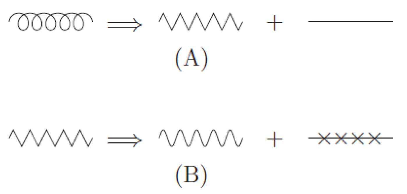
We can express the Abelian decomposition graphically. This is shown in Figure 1, where the gauge potential is decomposed to the restricted potential which has the full gauge degrees of freedom and the gauge covariant valence potential (the chromon) in (A), and the restricted potential is decomposed further to the non-topological Maxwell part (the neuron) and the topological Dirac part (the monopole) in (B).
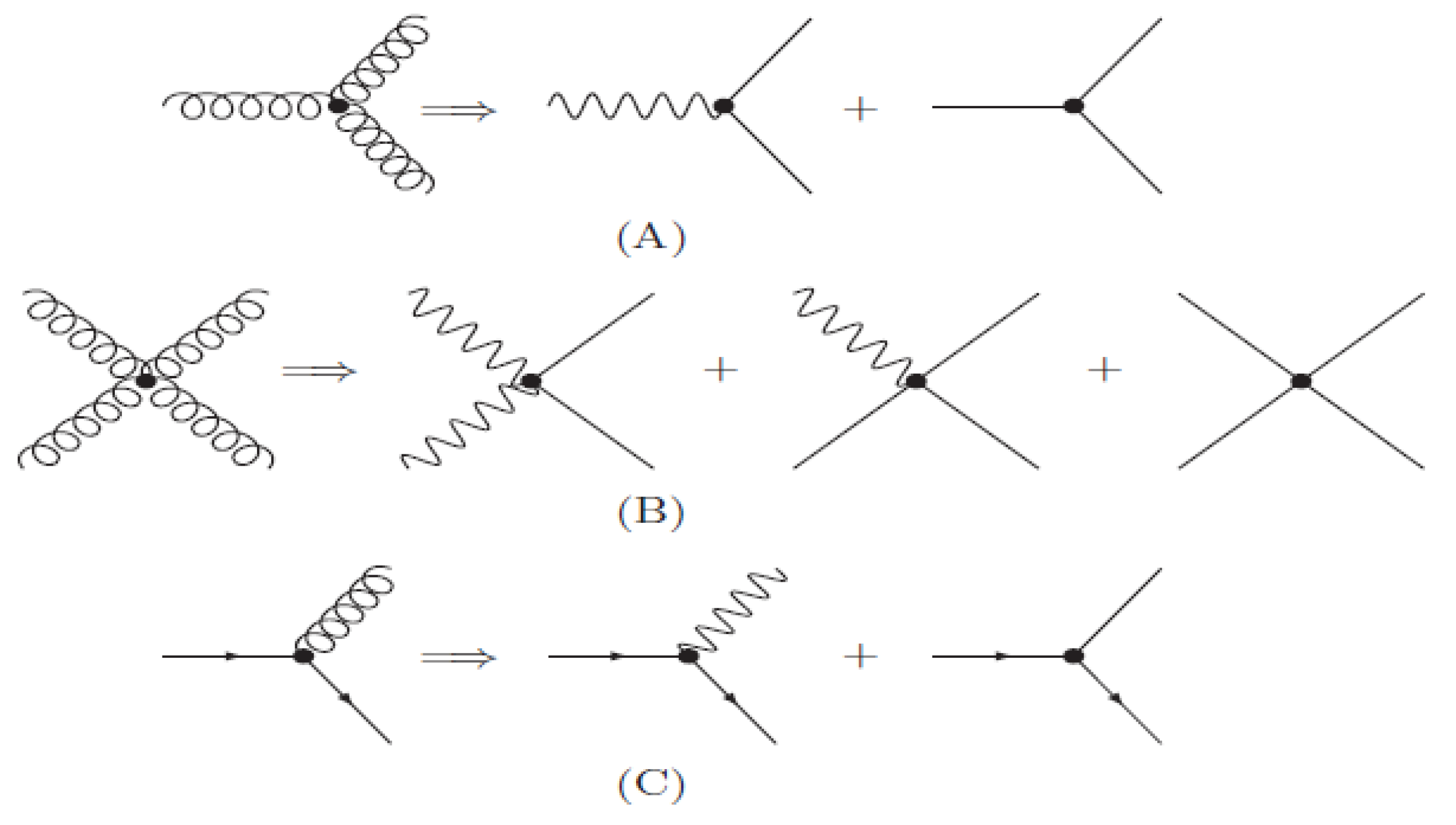
Although the Abelian decomposition does not change QCD, it reveals the important hidden characteristics of QCD. First, it shows that QCD has a non-trivial core RCD, which describes the Abelian sub-dynamics but has the full non-Abelian gauge symmetry. Moreover, it shows that QCD can be viewed as RCD which has the chromons as the colored source. Second, it shows the existence of two types of gluons, the neuron and chromon, which play totally different roles. This has deep implications. In the perturbative regime this tells that the Feynman diagram can be decomposed in such a way that the color conservation is explicit. This is graphically shown in Figure 2. In (A) the three-point gluon vertex is decomposed to two vertices, the one made of one neuron and two chromons and the other made of three chromons. In (B) the four-point gluon vertex is decomposed to three vertices made of one neuron and three chromons, two neurons and two chromons, and four chromons. In (C) the quark-gluon vertex is decomposed to the quark-neuron vertex and quark-chromon vertex.
It must be emphasized that this decomposition of the Feynman diagram is non-trivial. There is no three point vertex made of one chromon and two neurons, or three neurons. Similarly, there is no four point vertex made of one chromon and three neurons, or four neurons. They are forbidden by the conservation of color. In the conventional approach where all gluons are treated equal, there is no way to find this kind of hidden features of Feynman diagram. Please note that the monopole does not appear in the Feynman diagram, because it does not represent a dynamical degree. In fact we can always choose the trivial gauge (i.e., the gauge becomes a constant) where the monopole disappears completely.
The fact that the neurons and chromons play totally different roles is evident in (2) and (7). Clearly they show that the gauge covariant non-Abelian chromons, like the quarks, become the colored source of RCD. On the other hand the Abelian neurons, just like the photons in QED, play the role of the gauge potential which provides the binding for the colored source. This means that the neurons play the role of the binding gluons, while the chromons can be viewed as the valence gluons which become the constituent of hadrons. This naturally allows us to generalize the quark model to the quark and chromon model [32,33,34].
This plays important role to resolve the glueball problem in QCD. It has generally been believed that QCD has the glueballs made of gluons [46,47,48]. Several models of glueball have been proposed [49,50,51,52,53,54,55], and the Particle Data Group (PDG) has accumulated large number of hadronic states which do not seem to fit to the simple quark model as the glueball candidates [56].
Despite the huge efforts to identify the glueballs experimentally, however, so far the search for the glueballs has not been so successful for the following reasons [57,58,59,60,61]. First, theoretically there has been no consensus on how to construct the glueballs. This has made it difficult to predict what kind of glueballs we could expect. Second, it is not clear how to identify the glueballs experimentally. This is because they could mix with quarkoniums, so that we must take care of the possible mixing to identify the glueballs experimentally. This is why we have very few candidates of the glueballs so far, compared to huge hadron spectrum made of quarks listed in PDG.
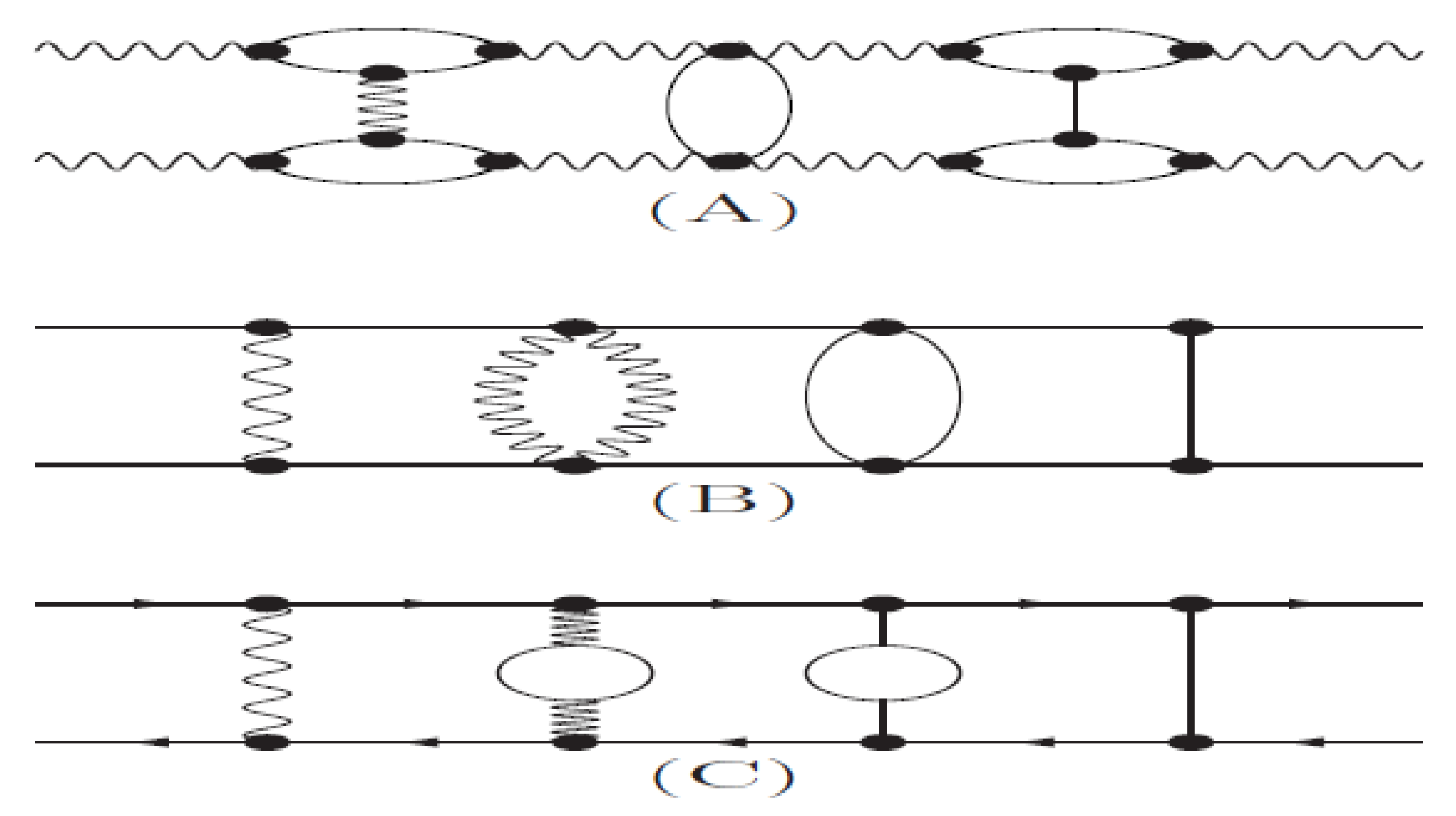
The quark and chromon model based on the Abelian decomposition provides a different picture of glueball, and could allow us to resolve the long-standing glueball problem. To see this consider the Feynman diagrams of two neurons, two chromons, and quark-antiquark pair shown in Figure 3. Remarkably, the neuron binding looks very much like the two photon binding in QED, while the chromon binding look just like the quark-antiquark binding in QCD. This strongly implies that the neurons can hardly make a bound state, so that they may not be viewed as the constituent of hadrons. However, the chromon binding shown in (B) strongly implies that they, just like the quarks, become the constituent of hadrons and form hadronic bound states which can be identified as the chromoballs. Moreover, together with quarks they could form new hybrid baryons. This leads us to the quark and chromon model which could provide a new picture of hadrons [32,33,34].
In particular, it provides a new picture of glueball different from all existing glueball models. In existing glueball models, all gluons are treated equally. However, the quark and chromon model tells that actually the chromoballs, the bound states of chromons, are identified as the glueballs [1,2,3,4,32,33,34]. Moreover, the model could describe the glueball-quarkonium mixing successfully. The numerical analysis of the mixing in , , and sectors below 2 GeV shows that in the sector , in the sector , and in the sector and could be identified as predominantly the glueball states [32,33,34].
To make the quark and chromon model work, however, we must tell what is the symmetry of the neurons and chromons, and how do they transform. Clearly the neurons and chromons cannot form the SU(3) octet, because they should not mix. This is the subject of the next section.
3. Color Reflection Symmetry
The Abelian decomposition is gauge independent. However, the selection of the Abelian direction amounts to the gauge fixing. So, once we fix the Abelian direction the gauge symmetry is broken. However, this does not break the gauge symmetry completely, so that we have the residual discrete symmetry called the color reflection symmetry after the Abelian decomposition [1,2,3,4].
The importance of this residual symmetry comes from the following observation. First, this plays the role of the gauge symmetry after the Abelian decomposition. Second, this symmetry is much simpler than the color gauge symmetry. This tells that the Abelian decomposition reduces the complicated non-Abelian gauge symmetry to a simple discrete symmetry which is much easier to handle. This greatly helps us to implement the gauge invariance in the calculation of the QCD effective action. So we discuss the color reflection symmetry first.
Consider the SU(2) QCD first, and make the color reflection, the -rotation of the SU(2) basis along the -direction which inverts the color direction ,
Obviously this is a gauge transformation which should not change the physics. On the other hand, under the color reflection (21) we have [30,32,33,34]
Moreover,
or by
in the complex notation.
However, since the isometry condition (2) is insensitive to (21), we have two different Abelian decompositions imposing the same isometry,
without changing the physics. This is why the color reflection (21) becomes a discrete symmetry of QCD after the Abelian decomposition [1,2,3,4].
To understand the meaning of this, notice that the neuron potential change the signature, while the topological part remains invariant. Moreover the chromon changes to the complex conjugate partner (together with the change of the signature), which changes the chromon to anti-chromon and flips the sign of the chromon charge. This is not surprising. In the absence of the topological part (7) describes QED which is coupled to the massless charged vector field where the neuron plays the role of the photon. In addition, in QED it is well known that the photon has negative charge conjugation. So it is natural that in SU(2) QCD changes the signature under the color reflection. Similarly we can argue that changes the signature under the parity [30,31].
On the other hand the monopole potential remains unchanged under the color reflection. This means that the monopole and anti-monopole are physically undistinguishable in QCD [35,36]. This should be contrasted with the monopole in spontaneously broken gauge theories, where the monopole and anti-monopole are physically different.
This confirms that although there are two possible magnetic backgrounds, only the monopole background coming from is qualified to be the legitimate background we can choose in the calculation of the QCD effective action. This is because changes the signature under the color reflection and thus fails to be gauge invariant. Indeed this is the reason the Savvidy vacuum is not gauge invariant.
As importantly, (23) tells that the physics should not change when we change the chromon to anti-chromon. In fact (23) tells that the chromon and anti-chromon are the color reflection partner. This means that they cannot be separately discussed in QCD and should always play exactly the same amount of role. This is the reason the color should become unphysical and confined, which makes QCD totally different from QED. This point plays a crucial role when we implement the gauge invariance in the calculation of the effective action [26,27,28,29,30,31].
In the fundamental representation the color reflection (21) is given by the 4 element subgroup of SU(2) made of [1,2,3,4]
This can be expressed by
which contains the diagonal subgroup made of and . This becomes the residual symmetry of the SU(2) quark doublet after the Abelian decomposition. Please note that plays the role of the generator of the color reflection group.
As for the gluons which form the adjoint representation the color reflection can be simplified further for the following reasons. First, the diagonal subgroup has no effect on the adjoint representation. Second, the color reflection changes to and to . So, the gluon triplet is decomposed to two independent representations. Indeed, for the neuron we have
However, for the chromon we have
or equivalently
in the complex notation. This confirms that the neuron and chromon transform independently, forming one-dimensional and two-dimensional representations under the color reflection. This drastically simplifies the non-Abelian gauge symmetry.
For SU(3) the fundamental representation the color reflection group is made of 24 elements subgroup of SU(3) given by [1,2,3,4,62]
where the four D-matrices form the diagonal subgroup. This describes the residual symmetry of the quark triplet after the Abelian decomposition. Please note that here and play the role of the generator. For example, we have , , and .
For the gluon octet which form the adjoint representation of SU(3) the color reflection can be simplified further. Just as in SU(2) QCD, the neurons and chromons transform separately, among themself. To see exactly how they transform notice that the two neurons and transform as
In terms of the (mutually dependent) triplet this translates to
This tells that basically represent the permutations of two SU(2) neurons with the signature change, but represent the cyclic permutations of three SU(2) neurons.
To find how the chromons transform we introduce the complex notation
and express the chromon sextet by . For the sextet we can show that the color reflection acts as follows,
Here denote the anti-chromon transformation (complex conjugation) plus permutations of two chromons, but denote the cyclic permutations of three chromons (up to the signature change). Just as in SU(2) QCD here the complex conjugation (anti-chromon transformation) of the chromons in the color reflection plays the crucial role in the calculation of the effective action.
The above analysis reveals another important difference between the neuron and chromon. Clearly (3) tells that the neurons permute amomg themself, but (3) tells that the chromons transform to anti-chromons, under the color reflection. In other words, just like the photon in QED the neurons have no anti-neurons. In comparison the chromons have the anti-chromon partners. This is because the neurons are color neutral, while the chromons are colored.
At this point one might wonder if there is any relation between the color reflection group and Weyl group. For SU(3), the Weyl group is the six elements permutation group of three colors which has a three-dimensional representation given by
which contains the cyclic made of and .
This tells that the two groups are different. They have different origin. The Weyl group comes as the symmetry of the Abelian decomposition, but the color reflection group comes as the residual symmetry of the Abelian decomposition. Unlike the color reflection group (29), the Weyl group (34) is not a subgroup of SU(3). Moreover, the Weyl group has no complex conjugation operation which transforms the chromons to anti-chromons. On the other hand they have a common subgroup , the cyclic permutation group of three colors.
Both the color reflection group and the Weyl group play a fundamental role in hadron spectroscopy. Only the color reflection invariant and Weyl invariant combinations of quarks and gluons can become physical in the quark and chromon model [32,33,34]. Moreover, they play the crucial role for us to demonstrate the monopole condensation gauge independently.
4. Color Reflection Invariance and Monopole Condensation
We have shown that in the perturbative regime, the Abelian decomposition plays important roles. It also plays the crucial role in the non-perturbative regime. First of all, it allows us to prove not only the Abelian dominance but also the monopole dominance in QCD rigorously. Obviously the chromons cannot play any role in the confinement, because they themselves have to be confined. This can be proved theoretically. First, we can prove that only the restricted potential contributes to the Wilson loop integral which generates the linear confining potential [9]. This is the Abelian dominance.
Furthermore, we can show that actually the monopole part of the restricted potential is responsible for the confining potential. Intuitively this is easy to understand. The Maxwell part (the neuron) plays the role of the electromagnetic potential in QED, which is known to have no confinement. This strongly implies the monopole dominance; that the monopole is responsible for the confinement.
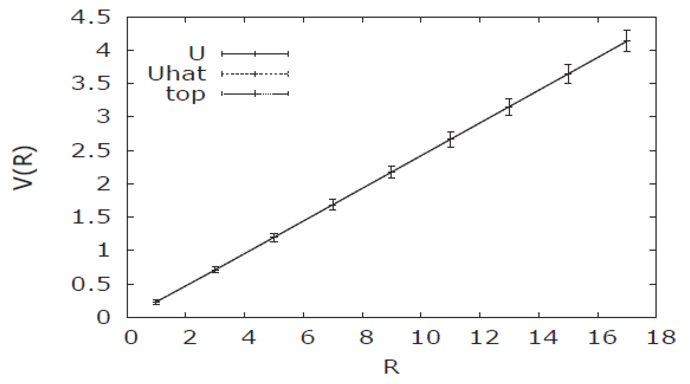
This is backed up numerically in the lattice QCD. Implementing the Abelian decomposition on the lattice, we can show that the confining force comes from the monopole part of the restricted potential [10,11,12,13,14,15]. The recent result of SU(3) lattice calculation is shown in Figure 4, which clearly shows that all three potentials, the full potential, the Abelian potential, and the monopole potential generate the same confining force. This establishes the monopole dominance.
The monopole dominance, however, does not tell us how the monopole confines the color. To tell how, we have to demonstrate the monopole condensation gauge independently. There have been many attempts to calculate the QCD effective action to prove the monopole condensation, which produced the magnetic condensation known as the Savvidy vacuum [16,17,18,19,20,21,22,23,24,25].
However, these calculations have many shortcomings. For example the separation of the classical part and the quantum part was not gauge independent. More seriously they have two critical mistakes. First, the Savvidy vacuum was unstable. This SNO instability was because they did not implement the gauge invariance properly in the calculation of the chromon functional determinant [26,27,28,29].
Second, the Savvidy vacuum was not gauge invariant, and thus cannot be the QCD vacuum. This was more critical than the SNO instability. This was because the old calculations did not understand the dual structure of RCD, and have chosen the non-topological Maxwell part as the background. This is not the monopole background. Worse, this is not gauge invariant [26,27,28,29,30,31].
The Abelian decomposition allows us to correct these defects and obtain the monopole condensation gauge independently. To show this it is important to understand that field theoretically ECD puts QCD in the background field formalism [37,38,45,63,64]. The background field formalism provides us an ideal platform to calculate the QCD effective action gauge independently. This is because the restricted potential and the valence potential can be treated as the slow varying classical field and the fluctuating quantum field, so that we can obtain the one-loop effective action of QCD integrating out the quantum part.
Specifically, the Abelian decomposition allows us to do the followings. First, it tells that RCD is made of two field strengths, the non-topological Maxwell part and the topological monopole part, and allows us to separate the monopole part gauge independently. As importantly, it tells that only the monopole part is gauge invariant and parity conserving, and thus is qualified to be the QCD vacuum. This was impossible in the old calculations because they could not separate the monopole part gauge independently.
Second, the Abelian decomposition simplifies the complicated non-Abelian gauge symmetry to the finite element color reflection symmetry as we have shown [1,2,3,4]. This makes the implementation of the gauge invariance much easier in the calculation of the chromon functional determinant when we integrate out the chromons. In particular, the the color reflection symmetry allows us to remove the tachyonic mode in the chromon functional determinant which made the SNO vacuum unstable. This makes the monopole condensation stable.
Moreover, the Abelian decomposition allows us to calculate the SU(3) QCD effective action directly from the SU(2) QCD effective action [30,31]. This is because the Abelian decomposition of SU(3) QCD transforms it to a Weyl symmetric form of three SU(2) QCD. This is evident in (2). This Weyl symmetry greatly simplifies the calculation of the SU(3) QCD effective action, and allows us to obtain the SU(3) QCD (or in general SU(N) QCD) effective action directly from the SU(2) QCD effective action.
Indeed, treating RCD as the classical part and choosing the monopole background, we can integrate out the chromons gauge independently and obtain the effective potential of RCD. The result shows that the true minimum of the RCD effective potential is given by the Weyl symmetric monopole condensation, with [30,31,32,34]. The SU(3) RCD effective potential is shown in Figure 5.
5. Neuron Jet and Chromon Jet at LHC
The Abelian decomposition is not just a theoretical proposition. It can be tested experimentally. There are various ways, but a straightforward and direct way is to confirm the existence of two types of gluons, the neurons and chromons, experimentally.
Theoretically there is no doubt that there exist two types of gluons which play totally different roles. Two types of gluons means two types of gluon jets, the neuron jet and chromon jet. As we have seen the neurons behave like photons in QED, while the chromons behave like the quarks in QCD. This implies that in the perturbative regime (i.e., in short distance) the neuron jet should behave like the photon jet, but the chromon jet should behave like the quark jet. So we could distinguish them and prove the existence of two types of gluon jets experimentally at LHC [32,33,34].
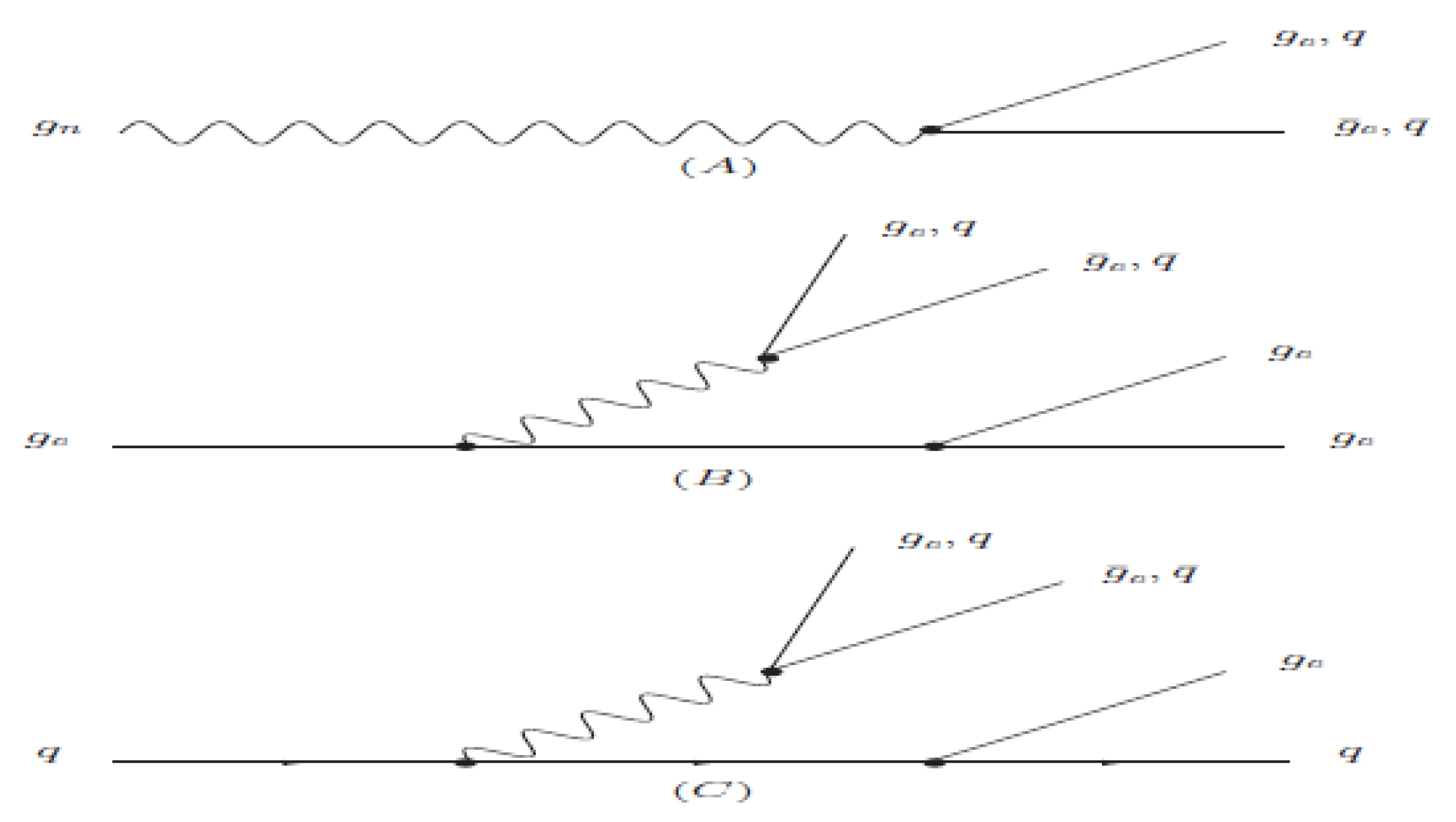
The gluons and quarks emitted in the p-p collisions evolve into hadron jets in two steps, the parton shower described by the perturbative process and the hadronization described by the non-perturbative process. The neuron and chromon behave differently in the first step. This is shown in Figure 6. Clearly the chromon jet shown in (B) and the quark jet shown in (C) look almost the same. However, the neuron jet shown in (A) has no parton shower made by neuron emission which exists in (B) and (C). This is because the three-point vertex made of three neurons is forbidden in QCD. This strongly suggests that the neuron jet must be sharper and has smaller radius.
To quantify the differences, we have to know the color factors of neurons and chromons, a most important quantity which characterizes the jet. We can argue that the color factor of the adjoint representation of SU(3) is divided to for the neurons and for the chromons, while the color factor of quarks remain the same. This means that .
There are other differences. Clearly the chromons and quarks carry color charge, but the neurons are color neutral. So the neuron jet must have different color factor and different color flow. Moreover, it could have different charged particle multiplicity. This means that the neuron jet must be qualitatively different from the chromon and quark jets, although we need theoretical calculations to tell the difference in detail.
Recently there has been huge progress on jet physics. Theoretically new features of the jet substructure have been known which can tell how to differentiate the gluon jet from the quark jet [65,66,67,68,69,70,71,72,73,74]. It is generally believed that because of different color factors in and vertices, the gluons have more parton radiation and thus make broader jets. Moreover, ATLAS and CMS have succeeded to separate the gluon jets and quark jets experimentally [75,76,77,78,79,80,81].
Now, the Abelian decomposition tells that we must have two different gluon jets. If so, what are the gluon jets identified by ATLAS and CMS? Probably they are the chromon jets. However, why have they not found two different gluon jets? Most likely they have not searched for the neuron jet yet, because they had no motivation do do that. LHC produces billions of hadron jets in a second, so that just by analizing the existing data they could find the neuron jets. They have succeeded the differentiate the chromon jets from the quark jets. Our analysis tells that it might be much easier to identify the neuron jets. This is clear from Figure 6. The Abelian decomposition provides a real motivation for them to do so.
The confirmation of the gluon jet has justifed the asymptotic freedom in QCD and extended our knowledge of QCD very much [82,83]. The experimental confirmation of two types of gluon jets would be at least as important. It will shed a new light on QCD revealing the hidden structures of QCD, and justify the quark and chromon model [32,33,34].
6. Discussion
In this paper we have discussed the color reflection symmetry, the fundamental symmetry of the quark and chromon model in QCD, which replaces the color gauge symmetry after the Abelian decomposition and plays the crucial role in hadron spectroscopy.
The Abelian decomposition reveals important hidden structures of QCD. In the perturbative regime it decomposes the gluons to the color neutral neurons and the colored chromons, and decomposes the Feynman diagrams in such a way that the conservation of color is manifest [1,2,3,4]. In the non-perturbative regime it puts QCD to the background field formalism by decomposing QCD to the classical background (the restricted Abelian part) and fluctuating quantum part (the gauge covariant valence part), and allows us to demonstrate the monopole condensation gauge independently [26,27,28,29,30,31].
This has a deep impact on hadron spectroscopy. It generalizes the quark model to the quark and chromon model which provides a new picture of hadrons, in particular the glueballs and glueball-quarkonium mixing [32,33,34]. This is because the colored chromons (just like the quarks) become the constituent of hadrons, but the colorless neurons (just like the photons in QCD) plays the role of the binding gluons.
The Abelian decomposition provides a different picture of glueball. First, it separates the colored chromons from the color neutral neurons gauge independently. Second, it tells that the chromons, just like the quarks, become the colored constituent of hadrons while the neurons play the role of the binding gluons. This naturally generalizes the quark model to the quark and chromon model, and provides a simple picture of the glueball and glueball-quarkonium mixing. In particular, the glueballs become the color singlet bound states of chromons. This helps us to resolve the long standing glueball problem and to identify the glueballs experimentally [1,2,3,4,32,33].
To show how the quark and chromon model works, however, we have to tell how they form the color singlet hadrons. To do this we have to know how the quark and chromons transform under the color gauge group. Since the eight gluons are decomposed to two neurons and six chromons under the Abelian decomposition, the color SU(3) cannot describe the symmetry of neurons and chromons. They have a new symmetry, the color reflection symmetry which becomes the fundamental symmetry of the hadron spectroscopy.
Before we close, we emphasize that the Abelian decomposition is not just a theoretical proposition. It can be tested directly by experiments at LHC. The experimental confirmation of two types of gluons will be a most important achievement of QCD.
Funding
The work is supported in part by National Research Foundation of Korea funded by the Ministry of Education (Grants 2015-R1D1A1A0-1057578 and 2018-R1D1A1B0-7045163) and by the Center for Quantum Spacetime at Sogang University.
Conflicts of Interest
The author declares no conflict of interest.
References
- Cho, Y.M. Restricted gauge theory. Phys. Rev. D 1980, 21, 1080. [Google Scholar] [CrossRef]
- Duan, Y.S.; Ge, M.L. SU (2) gauge theory and electrodynamics of N moving magnetic monopoles. Sci. Sin. 1979, 11, 1072–1086. [Google Scholar]
- Cho, Y.M. Glueball spectrum in extended quantum chromodynamics. Phys. Rev. Lett. 1981, 46, 302–306. [Google Scholar] [CrossRef]
- Cho, Y.M. Extended gauge theory and its mass spectrum. Phys. Rev. D 1981, 23, 2415. [Google Scholar] [CrossRef]
- Nambu, Y. Strings, monopoles, and gauge fields. Phys. Rev. D 1974, 10, 4262. [Google Scholar] [CrossRef]
- Mandelstam, S. Vortices and quark confinement in non-Abelian gauge theories. Phys. Rep. 1976, 23, 245–249. [Google Scholar] [CrossRef]
- Polyakov, A.M. Quark confinement and topology of gauge theories. Nucl. Phys. B 1977, 120, 429–458. [Google Scholar] [CrossRef]
- Hooft, G. Topology of the gauge condition and new confinement phases in non-Abelian gauge theories. Nucl. Phys. B 1981, 190, 455–478. [Google Scholar] [CrossRef]
- Cho, Y.M. Abelian dominance in Wilson loops. Phys. Rev. D 2000, 62, 074009. [Google Scholar] [CrossRef]
- Cundy, N.; Cho, Y.M.; Lee, W.; Leem, J. The static quark potential from the gauge invariant Abelian decomposition. Phys. Lett. B 2014, 729, 192–198. [Google Scholar] [CrossRef]
- Cundy, N.; Cho, Y.M.; Lee, W.; Leem, J. The static quark potential from the gauge invariant Abelian decomposition. Nucl. Phys. B 2015, 895, 64–131. [Google Scholar] [CrossRef]
- Kato, S.; Kondo, K.I.; Murakamik, T.; Shibata, A.; Shinohara, T.; Ito, S. Lattice construction of Cho-Faddeev-Niemi decomposition and gauge-invariant monopole. Phys. Lett. B 2006, 632, 326–332. [Google Scholar] [CrossRef]
- Kato, S.; Kondo, K.I.; Murakamik, T.; Shibata, A.; Shinohara, T.; Ito, S. Compact lattice formulation of Cho-Faddeev-Niemi decomposition: String tension from magnetic monopoles. Phys. Lett. B 2007, 645, 67–74. [Google Scholar]
- Kato, S.; Kondo, K.I.; Murakamik, T.; Shibata, A.; Shinohara, T.; Ito, S. Compact lattice formulation of Cho-Faddeev-Niemi decomposition: Gluon mass generation and infrared Abelian dominance. Phys. Lett. B 2007, 653, 101–108. [Google Scholar]
- Kato, S.; Kondo, K.I.; Murakamik, T.; Shibata, A.; Shinohara, T.; Ito, S. New descriptions of lattice SU (N) Yang–Mills theory towards quark confinement. Phys. Lett. B 2009, 669, 107–118. [Google Scholar]
- Savvidy, G.K. Infrared instability of the vacuum state of gauge theories and asymptotic freedom. Phys. Lett. B 1977, 71, 133–134. [Google Scholar] [CrossRef]
- Nielsen, N.; Olesen, P. An unstable Yang-Mills field mode. Nucl. Phys. B 1978, 144, 376–396. [Google Scholar] [CrossRef]
- Nielsen, N.; Olesen, P. A quantum liquid model for the QCD vacuum: Gauge and rotational invariance of domained and quantized homogeneous color fields. Nucl. Phys. B 1979, 130, 380–396. [Google Scholar] [CrossRef]
- Rajiadakos, C. A stable symmetrized Savvidy vacuum. Phys. Lett. B 1981, 100, 471–475. [Google Scholar] [CrossRef]
- Dittrich, W.; Reuter, M. Effective QCD-Lagrangian with ξ-function regularization. Phys. Lett. B 1983, 128, 321–326. [Google Scholar] [CrossRef]
- Reuter, M.; Dittrich, W. Symmetry restoration by a magnetic field at high temperature. Phys. Lett. B 1984, 144, 99–104. [Google Scholar] [CrossRef]
- Reuter, M.; Schmidt, M.G.; Schubert, C. Constant External Fields in Gauge Theory and the Spin 0, 12, 1 Path Integrals. Ann. Phys. 1997, 259, 313–365. [Google Scholar] [CrossRef]
- Yildiz, A.; Cox, P.H. Vacuum behavior in quantum chromodynamics. Phys. Rev. D 1980, 21, 1095–1099. [Google Scholar] [CrossRef]
- Claudson, M.; Yildiz, A.; Cox, P.H. Vacuum behavior in quantum chromodynamics. II. Phys. Rev. D 1980, 22, 2022–2026. [Google Scholar] [CrossRef]
- Ambjorn, J.; Hughes, R.J. Particle creation in colour-electric fields. Phys. Lett. B 1982, 113, 305–310. [Google Scholar] [CrossRef]
- Cho, Y.M.; Pak, D.G. Monopole condensation in SU (2) QCD. Phys. Rev. D 2002, 65, 074027. [Google Scholar] [CrossRef]
- Cho, Y.M.; Lee, H.W.; Pak, D.G. Faddeev–Niemi conjecture and effective action of QCD. Phys. Lett. B 2002, 525, 347–354. [Google Scholar] [CrossRef]
- Cho, Y.M.; Walker, M.L.; Pak, D.G. Monopole condensation and dimensional transmutation in SU (2) QCD. J. High Energy Phys. 2004, 2004, 073. [Google Scholar] [CrossRef]
- Cho, Y.M.; Walker, M.L. Stability of monopole condensation in SU (2) QCD. Mod. Phys. Lett. A 2004, 19, 2707–2716. [Google Scholar] [CrossRef]
- Cho, Y.M.; Cho, F.H.; Yoon, J.H. Dimensional transmutation by monopole condensation in QCD. Phys. Rev. D 2013, 87, 085025. [Google Scholar] [CrossRef]
- Cho, Y.M.; Cho, F.H. Abelian Decomposition and Weyl Symmetric Effective Action of SU(3) QCD. Phys. Rev. D 2019, in press. [Google Scholar]
- Cho, Y.M.; Pham, X.Y.; Zhang, P.; Xie, J.J.; Zou, L.P. Glueball physics in QCD. Phys. Rev. D 2015, 91, 114020. [Google Scholar] [CrossRef]
- Cho, Y.M. Quark and Chromon Model and Glueball-Quarkonium Mixing in QCD. Euro. Phys. J. WoC 2018, 182, 02031. [Google Scholar] [CrossRef]
- Zhang, P.; Zou, L.P.; Cho, Y.M. Abelian decomposition and glueball-quarkonium mixing in QCD. Phys. Rev. D 2018, 98, 096015. [Google Scholar] [CrossRef]
- Cho, Y.M. Colored monopoles. Phys. Rev. Lett. 1980, 44, 1115. [Google Scholar] [CrossRef]
- Cho, Y.M. Internal structure of the monopoles. Phys. Lett. B 1982, 115, 125–128. [Google Scholar] [CrossRef]
- De Witt, B. Dynamical theory of groups and fields. Relativity, groups and topology. Phys. Rev. 1967, 162, 1195. [Google Scholar]
- De Witt, B. Quantum theory of gravity. 3. Applications of the covariant theory. Phys. Rev. 1967, 162, 1239. [Google Scholar] [CrossRef]
- Faddeev, L.; Niemi, A.J. Partially dual variables in SU (2) Yang-Mills theory. Phys. Rev. Lett. 1999, 82, 1624. [Google Scholar] [CrossRef]
- Faddeev, L.; Niemi, A.J. Partial duality in SU (N) Yang-Mills theory. Phys. Lett. B 1999, 449, 214–218. [Google Scholar] [CrossRef]
- Shabanov, S.V. An effective action for monopoles and knot solitons in Yang-Mills theory. Phys. Lett. B 1999, 458, 322–330. [Google Scholar] [CrossRef]
- Shabanov, S.V. Yang-Mills theory as an Abelian theory without gauge fixing. Phys. Lett. B 1999, 463, 263–272. [Google Scholar] [CrossRef]
- Gies, H. Wilsonian effective action for SU (2) Yang-Mills theory with the Cho-Faddeev-Niemi-Shabanov decomposition. Phys. Rev. D 2001, 63, 125023. [Google Scholar] [CrossRef]
- Zucchini, R. Global aspects of abelian and center projections in SU (2) gauge theory. Int. J. Geom. Meth. Mod. Phys. 2004, 1, 813–846. [Google Scholar] [CrossRef]
- Bae, W.S.; Cho, Y.M.; Kimm, S.W. Extended QCD versus Skyrme-Faddeev theory. Phys. Rev. D 2001, 65, 025005. [Google Scholar] [CrossRef]
- Fritzsch, H.; Minkowski, P. ψ-resonances, gluons and the Zweig rule. Il Nuovo Cimento A 1975, 30, 393–429. [Google Scholar] [CrossRef]
- Freund, P.G.; Nambu, Y. Dynamics of the Zweig-Iizuka Rule and a New Vector Meson below 2 GeV/c 2. Phys. Rev. Lett. 1975, 34, 1645–1649. [Google Scholar] [CrossRef]
- Kogut, J.; Sinclair, D.K.; Susskind, L. A quantitative approach to low-energy quantum chromodynamics. Nucl. Phys. B 1976, 114, 199–236. [Google Scholar] [CrossRef]
- Chodos, A.; Jaffe, R.L.; Johnson, K.; Thorn, C.B.; Weisskopf, V.F. New extended model of hadrons. Phys. Rev. D 1974, 9, 3471. [Google Scholar] [CrossRef]
- Jaffe, R.L.; Johnson, K. Unconventional states of confined quarks and gluons. Phys. Lett. B 1976, 60, 201–204. [Google Scholar] [CrossRef]
- Roy, P.; Walsh, T.F. Spotting glueballs in collinear gluon jets. Phys. Lett. B 1978, 78, 62–66. [Google Scholar] [CrossRef]
- Shifman, M.A.; Vainshtein, A.I.; Zakharov, V.I. QCD and resonance physics. Theoretical foundations. Nucl. Phys. B 1979, 147, 385–447. [Google Scholar] [CrossRef]
- Coyne, J.J.; Fishbane, P.M.; Meshkov, S. Glueballs: Their spectra, production and decay. Phys. Lett. B 1980, 91, 259–264. [Google Scholar] [CrossRef]
- Chanowitz, M. Have We Seen Our First Glueball? Phys. Rev. Lett. 1981, 46, 981. [Google Scholar] [CrossRef]
- Cornwall, J.M.; Soni, A. Glueballs as bound states of massive gluons. Phys. Lett. B 1983, 120, 431–435. [Google Scholar] [CrossRef]
- Olive, K.A.; Particle Data Group. Review of particle physics. Chin. Phys. C 2014, 38, 090001. [Google Scholar] [CrossRef]
- Amsler, C.; Törnqvist, N.A. Mesons beyond the naive quark model. Phys. Rep. 2004, 389, 61–117. [Google Scholar] [CrossRef]
- Bugg, D.V. Four sorts of meson. Phys. Rep. 2004, 397, 257–358. [Google Scholar] [CrossRef]
- Klempt, E.; Zaitsev, A. Glueballs, hybrids, multiquarks: Experimental facts versus QCD inspired concepts. Phys. Rep. 2007, 454, 1–202. [Google Scholar] [CrossRef]
- Mathieu, V.; Kochelev, N.; Vento, V. The Physics of Glueballs. Int. J. Mod. Phys. E 2009, 18, 1–48. [Google Scholar] [CrossRef]
- Ochs, W. The status of glueballs. J. Phys. G Nucl. Part. Phys. 2013, 40, 043001. [Google Scholar] [CrossRef]
- Kondo, K.I.; Kato, S.; Shibata, A.; Shinohara, T. Quark confinement: Dual superconductor picture based on a non-Abelian Stokes theorem and reformulations of Yang-Mills theory. Phys. Rep. 2015, 579, 1–226. [Google Scholar] [CrossRef]
- Itzikson, C.; Zuber, J. Quantum Field Theory; McGraw-Hill: New York, NY, USA, 1985. [Google Scholar]
- Peskin, M.; Schroeder, D. An Introduction to Quantum Field Theory; Addison-Wesley: Boston, MA, USA, 1996. [Google Scholar]
- Fodor, Z. How to see the differences between quark and gluon jets. Phys. Rev. D 1990, 41, 1726. [Google Scholar] [CrossRef]
- Jones, L. Towards a systematic jet classification. Phys. Rev. D 1990, 42, 811. [Google Scholar] [CrossRef]
- Lonnblad, L.; Peterson, C.; Rognvaldsson, T. Using neural networks to identify jets. Nucl. Phys. B 1991, 349, 675–702. [Google Scholar] [CrossRef]
- Pumplin, J. How to tell quark jets from gluon jets. Phys. Rev. D 1991, 44, 2025. [Google Scholar] [CrossRef]
- Gallicchio, J.; Schwartz, M.D. Quark and Gluon Tagging at the LHC. Phys. Rev. Lett. 2011, 107, 172001. [Google Scholar] [CrossRef]
- Larkoski, A.J.; Salam, G.P.; Thaler, J. Energy correlation functions for jet substructure. J. High Energy Phys. 2013, 2013, 108. [Google Scholar] [CrossRef]
- Bhattacherjee, B.; Mukhopadhyay, S.; Nojiri, M.M.; Sakaki, Y.; Webber, B.R. Associated jet and subjet rates in light-quark and gluon jet discrimination. J. High Energy Phys. 2015, 2015, 131. [Google Scholar] [CrossRef]
- De Lima, D.F.; Petrov, P.; Soper, D.; Spannowsky, M. Quark-gluon tagging with shower deconstruction: Unearthing dark matter and Higgs couplings. Phys. Rev. D 2017, 95, 034001. [Google Scholar] [CrossRef]
- Davighi, J.; Harris, P. Fractal based observables to probe jet substructure of quarks and gluons. Eur. Phys. J. C 2018, 78, 1–8. [Google Scholar] [CrossRef]
- Metodiev, E.M.; Thaler, J. Jet Topics: Disentangling Quarks and Gluons at Colliders. Phys. Rev. Lett. 2018, 120, 241602. [Google Scholar] [CrossRef] [PubMed]
- ATLAS Collaboration. Measurement of jet shapes in top-quark pair events at = 7 TeV using the ATLAS detector. Eur. Phys. J. C 2013, 73, 2676. [Google Scholar] [CrossRef] [PubMed]
- ATLAS Collaboration. Light-quark and gluon jet discrimination in pp collisions at = 7 TeV with the ATLAS detector. Eur. Phys. J. C 2014, 74, 3023. [Google Scholar] [CrossRef] [PubMed]
- ATLAS Collaboration. Jet energy measurement and its systematic uncertainty in proton–proton collisions at = 7 TeV with the ATLAS detector. Eur. Phys. J. C 2015, 75, 17. [Google Scholar] [CrossRef] [PubMed]
- CMS Collaboration. Measurement of electroweak production of two jets in association with a Z boson in proton–proton collisions at = 8 TeV. Eur. Phys. J. C 2015, 75, 66. [Google Scholar] [CrossRef] [PubMed]
- CMS Collaboration. Search for the standard model Higgs boson produced through vector boson fusion and decaying to . Phys. Rev. D 2015, 92, 032008. [Google Scholar] [CrossRef]
- ATLAS Collaboration. Measurement of the charged-particle multiplicity inside jets from = 8 TeV pp collisions with the ATLAS detector. Eur. Phys. J. C 2016, 76, 1–23. [Google Scholar]
- ATLAS Collaboration. Jet energy scale measurements and their systematic uncertainties in proton-proton collisions at = 13 TeV with the ATLAS detector. Phys. Rev. D 2017, 96, 072002. [Google Scholar] [CrossRef]
- Gross, D.J.; Wilczek, F. Ultraviolet behavior of non-abelian gauge theories. Phys. Rev. Lett. 1973, 30, 1343. [Google Scholar] [CrossRef]
- Politzer, H.D. Reliable perturbative results for strong interactions? Phys. Rev. Lett. 1973, 30, 1346–1349. [Google Scholar] [CrossRef]
Figure 1.
The Abelian decomposition of the gauge potential. In (A) it is decomposed to the restricted potential (kinked line) and the chromon (straight line). In (B) the restricted potential is further decomposed to the neuron (wiggly line) and the monopole (spiked line).
Figure 1.
The Abelian decomposition of the gauge potential. In (A) it is decomposed to the restricted potential (kinked line) and the chromon (straight line). In (B) the restricted potential is further decomposed to the neuron (wiggly line) and the monopole (spiked line).

Figure 2.
The decomposition of the Feynman diagrams in SU(3) QCD. In (A,B) the three-point and four-point gluon vertices are decomposed, and in (C) the quark-gluon vertices are decomposed.
Figure 2.
The decomposition of the Feynman diagrams in SU(3) QCD. In (A,B) the three-point and four-point gluon vertices are decomposed, and in (C) the quark-gluon vertices are decomposed.

Figure 3.
The possible Feynman diagrams of the neurons and chromons. Two neuron interaction is shown in (A), two chromon interaction is shown in (B), and quark-antiquark interaction is shown in (C).
Figure 3.
The possible Feynman diagrams of the neurons and chromons. Two neuron interaction is shown in (A), two chromon interaction is shown in (B), and quark-antiquark interaction is shown in (C).

Figure 4.
The SU(3) lattice QCD calculation which establishes the monopole dominance in the confining force in Wilson loop integral. Here the confining forces shown in full, dashed, and dotted lines are obtained with the full potential, the Abelian potential, and the monopole potential, respectively.

Figure 5.
The SU(3) RCD effective potential which has a unique minimum at . Here H and represent the monopole field strength of two Abelian directions and . When they are orthogonal in real space, the potential has the true minimum.
Figure 5.
The SU(3) RCD effective potential which has a unique minimum at . Here H and represent the monopole field strength of two Abelian directions and . When they are orthogonal in real space, the potential has the true minimum.

Figure 6.
The perturbative diagrams of neuron, chromon, and quark jets. The neuron jet described in (A) is qualitatively different from the chromon jet and the quark jet shown in (B,C), while the chromon jet in (B) and the quark jet in (C) are qualitatively similar.
Figure 6.
The perturbative diagrams of neuron, chromon, and quark jets. The neuron jet described in (A) is qualitatively different from the chromon jet and the quark jet shown in (B,C), while the chromon jet in (B) and the quark jet in (C) are qualitatively similar.

© 2019 by the author. Licensee MDPI, Basel, Switzerland. This article is an open access article distributed under the terms and conditions of the Creative Commons Attribution (CC BY) license (http://creativecommons.org/licenses/by/4.0/).
Share and Cite
MDPI and ACS Style
Cho, Y. Two Types of Jets and Quark and Chromon Model in QCD. Universe 2019, 5, 62. https://0-doi-org.brum.beds.ac.uk/10.3390/universe5020062
AMA Style
Cho Y. Two Types of Jets and Quark and Chromon Model in QCD. Universe. 2019; 5(2):62. https://0-doi-org.brum.beds.ac.uk/10.3390/universe5020062
Chicago/Turabian StyleCho, Yongmin. 2019. "Two Types of Jets and Quark and Chromon Model in QCD" Universe 5, no. 2: 62. https://0-doi-org.brum.beds.ac.uk/10.3390/universe5020062
Note that from the first issue of 2016, this journal uses article numbers instead of page numbers. See further details here.