Langer Modification, Quantization Condition and Barrier Penetration in Quantum Mechanics

Abstract

The WKB approximation plays an essential role in the development of quantum mechanics and various important results have been obtained from it. In this paper, we introduce another method, the so-called uniform asymptotic approximations, which is an analytical approximation method to calculate the wave functions of the Schrödinger-like equations, and it is applicable to various problems, including cases with poles (singularities) and multiple turning points. A distinguished feature of the method is that in each order of the approximations the upper bounds of the errors are given explicitly. By properly choosing the freedom introduced in the method, the errors can be minimized, which significantly improves the accuracy of the calculations. A byproduct of the method is to provide a very clear explanation of the Langer modification encountered in the studies of the hydrogen atom and harmonic oscillator. To further test our method, we calculate (analytically) the wave functions for several exactly solvable potentials of the Schrödinger equation, and then obtain the transmission coefficients of particles over potential barriers, as well as the quantization conditions for bound states. We find that such obtained results agree with the exact ones extremely well. Possible applications of the method to other fields are also discussed.

1. Introduction

A fundamental interest in quantum mechanics (QM) is to derive various physical quantities from the wave function of the Schrödinger equation. Because of the complexity of the equation, it is extremely difficult to conduct analytical analyses, and various approximation methods have been proposed. Among them, the WKB approximation has played an essential role in the development of QM and has been widely used in many fields of physics and chemistry [1,2,3,4,5,6]. In general, the one- dimensional Schrödinger equation reads,

$$\begin{array}{c}\hfill \frac{d^2\mathrm{\Psi }\left(x\right)}{d{x}^2}+\frac{2m}{{ħ}^2}\left(E-V\left(x\right)\right)\mathrm{\Psi }\left(x\right)=0,\end{array}$$

(1)

which describes a particle of mass m moving with total energy E in a potential $V\left(x\right)$. Subsequently, using the WKB approximations, the wave function $\mathrm{\Psi }\left(x\right)$ can be approximately written in the form

$$\begin{array}{c}\hfill \mathrm{\Psi }\left(x\right)\simeq \frac{ħ}{\sqrt{2\left|p\right(x\left)\right|}}exp\left[\pm \frac{i}{ħ}{\int }^{x}p\left(x^{\prime }\right)d{x}^{\prime }\right],\end{array}$$

(2)

where $p\left(x\right)=\sqrt{2m(E-V)}$ is the local momentum. The validity of the approximation is restricted to the regions where the WKB condition is fulfilled,

$$\begin{array}{c}\hfill \mathcal{Q}\equiv {ħ}^2\left|\frac{3p^{\prime 2}}{4p^4}-\frac{p^{″}}{2p^3}\right|\ll 1.\end{array}$$

(3)

In this way, one can treat the reduced Planck constant ℏ as a small parameter and extend the leading-order solution (2) to high-orders.

However, it is well known that the above condition can be violated or not fulfilled completely in many cases [1]. For example, the WKB condition is always violated around turning points ($p\left(x\right)=0$), at which both $\mathcal{Q}$ and the WKB wave function (2) diverge. In addition, the WKB condition is also violated around singular points (poles) of $p^2\left(x\right)$. For instance, for the radial Schrödinger equation, the effective potential $V\left(r\right)$ contains a centrifugal term

$$V_C\left(r\right)=\frac{{ħ}^{2}l(l+1)}{2m{r}^2},$$

(4)

which has a second-order pole at the origin $r=0$.

Table 1. Some exactly solvable potentials and the choices of $q\left(x\right)$. The exact energy eignvalue spectra for these solvable potentials can be found in [7].

Potentials	$\mathit{V}\left(\mathit{x}\right)$	$\mathit{q}\left(\mathit{x}\right)$
Hydrogen	$-\frac{e^2}{x}+\frac{{ħ}^{2}l(l+1)}{2m{x}^2}$	$-\frac{1}{4x^2}$
Harmonic oscillator	$\frac{1}{2}m{\omega }^2{x}^2+\frac{{ħ}^{2}l(l+1)}{2m{x}^2}$	$-\frac{1}{4x^2}$
Morse potential	$v_0{e}^{-2\alpha x}+v_1{e}^{-\alpha x}$	0
Pöschl-Teller potential	$\frac{v_0}{{cosh}^2\left(\alpha x\right)}$	$\frac{{\alpha }^2}{4{cosh}^2\left(\alpha x\right)}$
Eckart potential	$\frac{v_0}{{\sinh }^2\left(\alpha x\right)}+\frac{v_1}{\tanh \left(\alpha x\right)}$	$-\frac{{\alpha }^2}{4{\sinh }^2\left(\alpha x\right)}$

presents other typical potentials encountered in QM.

Note that it is exactly because of this second-order pole that the WKB approximation fails to give correct results for hydrogen atoms and harmonic oscillators [8]. This problem was studied by Langer several decades ago, and showed that it can be cured if one replaces $l(l+1)$ by ${(l+1/2)}^2$ in $V_C\left(r\right)$ [9]. This modification now is considered as a standard ingredient of the WKB method in QM [1]. However, a rigorous and logically consistent derivation of this modification is still lacking.

Another situation that could violate the WKB condition is around the extreme point of $p^2\left(x\right)$ if $\mathcal{Q}\simeq |p^{″}/2p^3|\sim \mathcal{O}\left(1\right)$. This can arise in the bound states with a potential well or in particle scattering with a potential barrier. In both cases, the results from the WKB approximation becomes invalid if $\mathcal{Q}$ is not small enough at the extreme points.

To overcome these problems, various (approximate) methods have been proposed [7], including the complex [10,11,12,13,14] and uniform WKB methods [9,15,16,17,18]. In the complex method, one first generalizes the above one-dimensional problem into a complex x plane, and then joins the two parts $x>a$ and $x<a$ by a path in the complex plane, which is sufficiently far from the turning point $x=a$, so the WKB solutions are valid along the path. With the seminal work of Delabaere, Dillinger and Pham [14], the long-standing problem of the method, the ambiguities of the unique matching between the two parts [1], was finally resolved. Consequently, a simple and rigorous justification of the Zinn–Justin quantization condition and its solution in terms of the “multi-instanton expansion” for the symmetric double well problem [19], were derived. On the other hand, the uniform (in the sense of being smooth across the turning points) WKB approximation method is a generalization of the basic WKB approximations by employing the technique of comparison equations [20,21]. In this approach, the solution is mapped on to the one of a simpler equation, which, however, has the same disposition of turning points as the original. Without bypassing the turning points, as done in the complex method [14], the uniform WKB approximations also provide the wave function in the neighborhood of the turning points. Using this method, Álvarez was also able to derive the “multi-instanton expansion” for the eigenvalues of the symmetric double well by using a Langer–Cherry uniform asymptotic expansion [17]. An excellent pedagogical introduction of this method was recently provided by Dunne and Ünsal with both the double well and the Sine–Gordon potentials as concrete examples [18], in which the relations among the uniform WKB approach, multi-instanton, and resurgence theory were also explored.

The purpose of this paper is to present another approximation method, the so-called uniform asymptotic approximation method, developed systematically by Olver [22,23]. Among other things, an essential difference of this method from the above ones is that explicit bounds are constructed for the error terms associated with the approximations, although, similar to the uniform WKB method, it is also based on the comparison equations [20,21]. In particular, we shall accurately calculate the wave function of the Schrödinger Equation (1) with singular potentials, such as those given in Table 1, although the method is quite general, and, in principle, can be applied to any problem of the Schrödinger Equation (1), including the cases with poles and multiple turning points. This method has been already shown to be powerful and robust when applied to calculations of the mode functions and primordial power spectra in a variety of slow-roll inflationary models [24,25,26,27,28,29], adiabatic regularization of the power spectra in various inflationary models [30,31], inflation with non-linear dispersion relations [32,33,34,35,36,37,38,39], and loop quantum cosmology [40,41,42,43], as well as studying the parametric resonance during inflation and reheating [44]. As mentioned above, the major advantage of the method is that the errors in each order of approximations can be estimated and the upper bounds of the errors are always known. In particular, for certain models, it was found that the errors are no larger than $0.15\%$ up to the third-order of approximations [36].

In the application of this method to hydrogen atoms and harmonic oscillators, we provide a rigorous derivation of the Langer modification and expressions for the quantization conditions and the barrier transmission coefficients. Applications of our method to some well-known examples are also presented, in order to further test it.

2. Uniform Asymptotic Approximation Method

2.1. Wave Functions in the Uniform Asymptotic Approximation

Let us first write the standard form of (1) in the form [22,23],

$$\begin{array}{c}\hfill \frac{d^2\mathrm{\Psi }\left(x\right)}{d{x}^2}=\left\{g\left(x\right)+q\left(x\right)\right\}\mathrm{\Psi }\left(x\right),\end{array}$$

(5)

where $g\left(x\right)+q\left(x\right)=-p^2\left(x\right)/{ħ}^2$. Note that, for any given $p\left(x\right)$, here we introduce two functions $g\left(x\right)$ and $q\left(x\right)$, and, to fix them uniquely, we require that the errors in each order of approximations be minimized. This is one of the major ingredients of the method. Subsequently, such defined $g\left(x\right)$, in general, can have zero points $g\left(x_i\right)=0$, which are called turning points in the uniform asymptotic approximation. Except such points, $g\left(x\right)$ may also have other types of transition points, such as poles and extreme points. According to the theory of the second-order ordinary differential equations [22,23], the wave function $\mathrm{\Psi }\left(x\right)$ sensitively depends on the number and nature of turning points, poles, and extreme points. Analyzing the corresponding error control function around poles and extreme points provides the main guidance on how to determine $g\left(x\right)$ and $q\left(x\right)$ [22,23]. In addition, around each of the turning points $x_i$, we require $\left|q\left(x\right)\right|\ll |g\left(x\right)/(x-x_i)|$, while away from them, we require $\left|q\right(x\left)\right|\ll \left|g\right(x\left)\right|$ [22,23].

At the turning points, the WKB condition (3) is violated, and the wave function (2) becomes invalid. Generally, the turning points can have different types, depending on the nature of the zeros of $g\left(y\right)$. The simplest case is the single turning point that denotes the simple and single zero of $g\left(y\right)$. Besides this, $g\left(y\right)$ may also have a pair of turning points, which could be both real and single, double, or even complex conjugated. In the following, we are going to construct the uniform wave function for above two cases individually.

2.1.1. For Single Turning Point

Let us first consider the single turning point, say, denoted by $x_0$. We can write the function $g\left(x\right)$ in the form of

$$\begin{array}{c}\hfill g\left(x\right)=f\left(x\right)(x-x_0),\end{array}$$

(6)

where $f\left(x\right)$ is a regular function. In quantum mechanics, this turning point can be thought as the critical point that separates the classically allowed and forbidden regions of a quantum system if $q\left(x\right)=0$. When we have to chose $q\left(x\right)\ne 0$, it will produce a small shift on this point. Around the turning point $x_0$, the wave function $\mathrm{\Psi }\left(x\right)$ can be written as [23]

$$\begin{array}{c}\hfill \mathrm{\Psi }\left(x\right)={\left(\frac{\xi \left(x\right)}{g\left(x\right)}\right)}^{1/4}\left(a_0\mathrm{Ai}\left(\xi \right)+b_0\mathrm{Bi}\left(\xi \right)\right),\end{array}$$

(7)

where $\mathrm{Ai}\left(\xi \right)$ and $\mathrm{Bi}\left(\xi \right)$ are the Airy functions, $a_0$ and $b_0$ are two integration constants, and $\xi \left(x\right)$ is chosen to be a monotonic function of x, which has the same sign of $g\left(x\right)$ with relations $\sqrt{\left|\xi \right|}d\xi =\sqrt{\left|g\right(x\left)\right|}dx$ and $\xi \left(x_0\right)=0$. The errors are controlled by the error control function,

$$\begin{array}{c}\mathcal{H}\left(\xi \right)\equiv \frac{5}{{24\left|\xi \right|}^{3/2}}-{\int }_{x_0}^x\left\{\frac{q\left(\tilde{x}\right)}{g\left(\tilde{x}\right)}-\frac{5g^{\prime 2}\left(\tilde{x}\right)}{16g^3\left(\tilde{x}\right)}+\frac{g^{″}\left(\tilde{x}\right)}{4g^2\left(\tilde{x}\right)}\right\}\sqrt{\left|g\right(\tilde{x}\left)\right|}d\tilde{x}.\hfill \end{array}$$

(8)

2.1.2. A Pair of Turning Points

For a pair of turning points $x_1$ and $x_2$, they could be: (1) both real and different $x_1\ne x_2$; (2) both real but equal $x_1=x_2$; or, (3) complex conjugate $x_1=x_2^{*}$. In each case, between these points, $g\left(y\right)$ usually has one extreme.

If this extreme is a minimal point of $g\left(y\right)$, we can construct the wave function $\mathrm{\Psi }\left(x\right)$ in terms of the parabolic cylinder functions $U(-{\zeta }_0^2/2,\sqrt{2}\zeta )$ and $\overline{U}(-{\zeta }_0^2/2\sqrt{2}\zeta )$ as [22],

$$\begin{array}{ccc}\hfill \mathrm{\Psi }\left(x\right)& =& {\left(\frac{{\zeta }^2-{\zeta }_0^2}{-g\left(x\right)}\right)}^{1/4}\left(a_{1}U(-{\zeta }_0^2/2,\sqrt{2}\zeta )+b_1\overline{U}(-{\zeta }_0^2/2,\sqrt{2}\zeta )\right).\hfill \end{array}$$

(9)

If the extreme is a maximal point, then the wave function can also be constructed in terms of parabolic cylinder functions, but now in terms of $W({\zeta }_0^2/2,\sqrt{2}\zeta )$ and $W({\zeta }_0^2/2,-\sqrt{2}\zeta )$,

$$\begin{array}{ccc}\hfill \mathrm{\Psi }\left(x\right)& =& {\left(\frac{{\zeta }^2-{\zeta }_0^2}{-g\left(x\right)}\right)}^{1/4}\left(a_{2}W({\zeta }_0^2/2,\sqrt{2}\zeta )+b_{2}W({\zeta }_0^2/2,-\sqrt{2}\zeta )\right).\hfill \end{array}$$

(10)

In both cases, the variable $\zeta \left(x\right)$ is a monotonic function of x and is defined by $\sqrt{|{\zeta }^2-{\zeta }_0^2|}d\zeta =\sqrt{\left|g\right(x\left)\right|}dx$ with $\zeta \left(x_1\right)=-\left|{\zeta }_0\right|$, $\zeta \left(x_2\right)=\left|{\zeta }_0\right|$, and ${\zeta }_0^2=\pm (2/\pi )\left|{\int }_{x_1}^{x_2}\sqrt{\left|g\right(x\left)\right|}dx\right|$, where $“+”$$(“-”)$ corresponds to the case in which the two turning points $x_1$ and $x_2$ are real (complex conjugate). The associated error control function of the above two wave functions is,

$$\begin{array}{cc}\hfill \mathcal{I}\left(\zeta \right)=& {\int }_{\pm {\zeta }_0}^{\zeta }\left[\frac{5{\zeta }_0^2}{4|v^2-{\zeta }_0^2{|}^{5/2}}-\frac{3}{4|v^2-{\zeta }_0^2{|}^{3/2}}\right]dv\hfill \\ & -{\int }_{x_{1,2}}^x\left\{\frac{q\left(\tilde{x}\right)}{g\left(\tilde{x}\right)}-\frac{5g^{\prime 2}\left(\tilde{x}\right)}{16g^3\left(\tilde{x}\right)}+\frac{g^{″}\left(\tilde{x}\right)}{4g^2\left(\tilde{x}\right)}\right\}\sqrt{\left|g\right(\tilde{x}\left)\right|}d\tilde{x}.\hfill \end{array}$$

(11)

The wave functions given in (7), (9) and (10) are valid in the neighborhoods of the turning points $x_i$. The extension of them beyond these points crucially depends on the behaviors of the corresponding error control functions in the extended regions. In the following, let us consider it for the case with a second-order pole, as shown in (4).

2.2. Second-Order Pole and Langer Modification

As mentioned above, for the radial Schrödinger equation, the effective potential $V_C\left(r\right)$ given by (4) contains a second-order pole at the origin, at which we have $(\xi ,\zeta )\to \pm \infty$, and

$$\begin{array}{c}\hfill (\mathcal{H},\mathcal{I})\to -{\int }^x\left(\frac{q}{g}-\frac{5g^{\prime 2}}{16g^3}+\frac{g^{″}}{4g^2}\right)\sqrt{\left|g\right|}dx.\end{array}$$

(12)

Because, near the second-order pole, $g\left(x\right)$ has the asymptotic behavior

$$g\left(x\right)\sim a/x^2,$$

(13)

we find that the error control function takes the limit

$$\begin{array}{c}\hfill \left(\mathcal{H},\mathcal{I}\right)\to \underset{x\to 0}{lim}\left(-\frac{lnx}{4\sqrt{\left|a\right|}}-{\int }^x\frac{q}{\sqrt{\left|g\right|}}dx\right).\end{array}$$

(14)

In order to make our analytic solutions in (7), (9) and (10) also valid at the origin, we must require that the error control function given by (14) are finite at the pole $x=0$. Using the asymptotic behavior of $g\left(x\right)$ given in (13), it is straightforward to show that the right-hand side of (14) can be made finite at the pole as long as [33]

$$q\left(x\right)=-\frac{1}{4x^2},$$

(15)

which is nothing but exactly the Langer modification. Thus, the latter is simply the result of imposing the condition that the error control function be finite at the pole in the uniform asymptotic approximation method.

2.3. Extreme Point and the Elimination of the Error Term

The extreme points of $g\left(x\right)$ in general arise from quantum system with a potential well or barrier in the region between two turning points. These extreme points are the same as the bottom of the well or the top of the potential if one chooses $q\left(x\right)=0$. As mentioned above, the existence of the extreme points will make the WKB approximation invalid if $\mathcal{Q}$ is not small enough at the extreme. Such cases arise when the potential wells or barriers are sharply peaked, for which $g\left(x\right)$ has two coalescent turning points $x_1$ and $x_2$. To be more specific, let us write $g\left(x\right)$ in the form

$$\begin{array}{c}\hfill g\left(x\right)=f\left(x\right)(x-x_1)(x-x_2),\end{array}$$

(16)

where $f\left(x\right)$ is a finite and regular function with $f\left(x_i\right)\ne 0$. Subsequently, we expect that the dominant contribution to the integral of (11) arises from the lower limit. Therefore, we can formally expand the error control function $\mathcal{I}\left(\zeta \right)$ about the turning points and find1,

$$\begin{array}{ccc}\hfill \mathcal{I}\left(\zeta \right)& \simeq & {\left.\frac{7f^{\prime 2}-6f{f}^{″}}{{32\left|f\right|}^{5/2}}\right|}_{\mathrm{Re}\left(x_i\right)}ln|x_2-x_1|-{\int }_{\mathrm{Re}\left(x_i\right)}\frac{q}{\sqrt{\left|g\right|}}dx,(i=1,2),\hfill \end{array}$$

(17)

where $\mathrm{Re}\left(x_i\right)$ denotes the real part of the turning point $x_i$. Note that, in deriving the above expression, we had ignored the small corrections. We also note that, when the turning points $x_1$ and $x_2$ are close to each other, the dominant contributions to the error control function come from the $ln|x_2-x_1|$ term, which becomes divergent at $x_1=x_2$. It is somehow surprising that such dominant contributions seemingly had never been noticed before, and later they will play an essential role in determining the extension of the wave functions to the regions near the extreme point.

With the knowledge of the error control function (17), we are now in a position to eliminate the dominant error term in (17) by properly choosing $q\left(x\right)$ in the second term of (17). To achieve this, we expand $q\left(x\right)$ at one of the turning points2,

$$\begin{array}{c}\hfill q\left(x\right)\simeq q_0+q_1(x-\mathrm{Re}\left(x_i\right)).\end{array}$$

(18)

Subsequently, the elimination of the first error term in (17) requires

$$\begin{array}{c}\hfill q_0={\left.\frac{7f^{\prime 2}-6f{f}^{″}}{32f^2}\right|}_{\mathrm{Re}\left(x_i\right)}.\end{array}$$

(19)

This represents one of the important conditions for the choice of the function $q\left(x\right)$. Additional requirements include that $\left|q\right(x\left)\right|$ be negligible in comparison with $\left|g\right(x\left)\right|$ in the regions that is away from the extreme and turning points. Subsequently, we expect that the right hand side of (19) does not contain $q_0$ and should be independent of the nature of the two turning points $x_1$ and $x_2$. For this requirement, one can relate $q_0$ to the derivatives of the function $g\left(x\right)$ at the extreme point $x_m$ via the relation,

$$\begin{array}{c}\hfill q_0={\left(\frac{7g^{‴2}}{288g^{″2}}-\left.\frac{g^{⁗}}{32g^{″}}\right)\right|}_{x_m}.\end{array}$$

(20)

3. Improved Quantization Conditions and Potential Barrier Transmission Coefficients

With the above considerations, now we are at the position to generalize the wave functions near poles and extreme points. These wave functions can then be utilized to derive the quantization conditions for bound states or the quantum transmission coefficients of a particle through a potential barrier. In this section, we are going to discuss quantization conditions and potential barrier transmission individually by using the quantum mechanical wave functions that were derived in the above section with the corresponding $q\left(x\right)$ calculated for specific potentials.

3.1. Improved Quantization Condition

One of the most important topics in quantum mechanics is to determine the bound states and energy eigenvalue spectra for a quantum mechanical system. As mentioned in the introduction, the conventional WKB method fails to describe the correct behaviors of wave functions around the poles, extreme points, and turning points of $E-V\left(x\right)$ in the Schrödinger Equation (1). Especially at the turning point, the WKB wave function (2) becomes divergent. One approach for avoiding this singularity is the complex method, in which the WKB approximation has been extended to the complex x plane. In this way, the two WKB wave functions in the classically allowed and forbidden regions can be connected without the knowledge of the wave functions around the turning points. With this procedure, when a particle is trapped in a potential well $V\left(x\right)$, the corresponding energy eigenvalue spectra can be obtained using the conventional WKB quantization condition,

$$\begin{array}{c}\hfill {\int }_{{\tilde{x}}_1}^{{\tilde{x}}_2}\sqrt{\frac{2m}{{ħ}^2}\left(E-V\left(x\right)\right)}dx=\left(n+\frac{1}{2}\right)\pi ,\end{array}$$

(21)

where ${\tilde{x}}_1$ and ${\tilde{x}}_2$ are two zeros of $E-V\left(x\right)$ (or classical turning points of (1)) and n denotes the quantum number. It is worth noting that ${\tilde{x}}_1$ and ${\tilde{x}}_2$ is slightly different from the turning points $x_1$ and $x_2$ of $g\left(y\right)$ with $q\left(x\right)\ne 0$. For one single turning point system, where a particle is trapped in a classically allowed for a region with a boundary at $x_b$, the WKB quantization gives,

$$\begin{array}{c}\hfill {\int }_{x_b}^{{\tilde{x}}_0}\sqrt{\frac{2m}{{ħ}^2}\left(E-V\left(x\right)\right)}dx=\left(n+\frac{3}{4}\right)\pi .\end{array}$$

(22)

However, in the uniform asymptotic approximations, if $g\left(x\right)$ has two turning points $x_1$ and $x_2$, the wave function (9) leads to the quantization condition,

$$\begin{array}{c}\hfill \frac{\pi {\zeta }_0^2}{2}={\int }_{x_1}^{x_2}\sqrt{-g\left(x\right)}=\left(n+\frac{1}{2}\right)\pi .\end{array}$$

(23)

When $g\left(x\right)$ has only one turning point $x_0$, the wave function (7) leads to the quantization condition,

$$\begin{array}{c}\hfill {\int }_{x_0}^{x_b}\sqrt{-g\left(x\right)}=\left(n+\frac{3}{4}\right)\pi ,\end{array}$$

(24)

where $x_b$ is the boundary of the classically allowed region. The above quantization condition is different from that derived in the WKB approximation, except for the case with $q\left(x\right)=0$. For the quantum mechanical system that $q\left(x\right)$ has to be nonzero, the above quantization condition can provide a significant improvement on the calculations of the energy eigenvalue spectra for a quantum mechanical system. In the following, for applications of the above quantization condition, we consider several representative exactly solvable systems, including hydrogen atoms, harmonic oscillators in D dimensions, Morse potential, Pöschl-Teller potential, and Eckart potential, as given in Table 1.

3.1.1. Hydrogen Atoms

For hydrogen atoms, the electron moves in the atom with a Coulomb potential and a centrifugal term [7],

$$\begin{array}{c}\hfill V\left(x\right)=-\frac{e^2}{x}+\frac{{ħ}^{2}l(l+1)}{2m{x}^2},\end{array}$$

(25)

where e denotes the electron charge. The Schrödinger Equation (1) of the hydrogen atom can be solved exactly, and from the exact solution one can easily obtain the exact energy eigenvalue spectra as [7]

$$\begin{array}{c}\hfill E_n=-\frac{m{e}^4}{2{ħ}^2{(n+l+1)}^2}.\end{array}$$

(26)

If we apply the WKB quantization condition (21), the WKB energy eigenvalue spectra read

$$\begin{array}{c}\hfill E_n=-\frac{m{e}^4}{2{ħ}^2{(n+1/2+\sqrt{l(l+1)})}^2},\end{array}$$

(27)

which does not match the exact result. A standard procedure to solve this problem in quantum mechanics can be implemented while using the Langer modifciation by simply replacing $l(l+1)$ by ${(l+1/2)}^2$ in the Schrödinger equation [9].

In the uniform asymptotic approximation, the above problem can be resolved by properly choosing $q\left(x\right)$ to eliminate the divergent errors of the approximate solution arising from the existence of the second-order pole and the extreme point. It can be seen that the Schrödinger Equation (1) for the hydrogen atom has a second order pole, one extreme point, and two turning points. Subsequently, according to the analysis in the above section, $q\left(x\right)$ has to be chosen, such that

$$\begin{array}{c}\hfill q\left(x\right)\to -\frac{1}{4x^2}\mathrm{as}x\to 0,\end{array}$$

(28)

$$\begin{array}{c}\hfill q\left(x_m\right)={\left(\frac{7g^{‴2}}{288g^{″2}}-\left.\frac{g^{⁗}}{32g^{″}}\right)\right|}_{x_m}.\end{array}$$

(29)

To meet these two conditions, $q\left(x\right)$ must be

$$\begin{array}{c}\hfill q\left(x\right)=-\frac{1}{4x^2}.\end{array}$$

(30)

With this choice, the two turning points $x_1$ and $x_2$ can be solved from $g\left(x\right)=0$, yielding

$$\begin{array}{c}\hfill x_1=-\frac{e^2}{2E}+\frac{\sqrt{m^2{E}^4+mE{(l+1/2)}^2{ħ}^2}}{2mE},\end{array}$$

(31)

$$\begin{array}{c}\hfill x_2=-\frac{e^2}{2E}-\frac{\sqrt{m^2{E}^4+mE{(l+1/2)}^2{ħ}^2}}{2mE}.\end{array}$$

(32)

Substituting them into the improved quantization condition (23), one immediately obtains

$$\begin{array}{c}\hfill E_n=-\frac{m{e}^4}{2{ħ}^2{(n+l+1)}^2},\end{array}$$

(33)

which precisely recovers the exact result. The eigenstate for each quantum number then is given by the wave function in (9) with $q\left(x\right)$ given in (30), which is uniformly valid in the whole region $x\in (0,+\infty )$. It is worth noting that the above analysis can be easily extended to the hydrogen-like atoms.

3.1.2. Harmonic Oscillators

The potential for the harmonic oscillator in D dimensions is given by [7]

$$\begin{array}{c}\hfill V\left(x\right)=\frac{1}{2}{m}^2{\omega }^2{x}^2+\frac{{ħ}^2}{2m{x}^2}\left(l\left(D+l-2\right)+\frac{(D-1)(D-3)}{4}\right).\end{array}$$

(34)

The exact solution of the Schrödinger Equation (1) with the above potential leads to [7]

$$\begin{array}{c}\hfill E_n=\left(2n+l+\frac{D}{2}\right)ħ\omega .\end{array}$$

(35)

If we perform the WKB quantization condition (21), the WKB energy eigenvalue spectra read

$$\begin{array}{c}\hfill E_n=\left(2n+\sqrt{l\left(D+l-2\right)+\frac{(D-1)(D-3)}{4}}+1\right)ħ\omega .\end{array}$$

(36)

Similar to the hydrogen atom, it does not match the exact result.

To execute the analysis in the uniform asymptotic approximation, we observe that Schrödinger Equation (1) for the harmonic oscillator in D dimensions has one second-order pole, one extreme point, and two turning points. This is very similar to the case in the hydrogen atom. Subsequently, the choice of $q\left(x\right)$ has to meet the two conditions in (28) and (29), which leads to

$$\begin{array}{c}\hfill q\left(x\right)=-\frac{1}{4x^2}.\end{array}$$

(37)

With this choice, the improved quantization condition (23) then gives

$$\begin{array}{c}\hfill E_n=\left(2n+l+\frac{D}{2}\right)ħ\omega ,\end{array}$$

(38)

which again recovers the exact result. Similarly, the eigenstate for each quantum number is given by the wave function in (9), which is valid in the whole region of interest.

3.1.3. Morse Potential

The Morse potential is given by [7]

$$\begin{array}{c}\hfill V\left(x\right)=v_0{e}^{-2\alpha x}+v_1{e}^{-\alpha x},\end{array}$$

(39)

where $v_0$, $v_1$, and $\alpha$ are three parameters in the potential. The exact solution of the Schrödinger Equation (1) with the Morse potential leading to the following energy eigenvalue spectra [7],

$$\begin{array}{c}\hfill E_n=-\frac{2m{v}_1^2+(2n+1)\alpha ħ(2\sqrt{2m{v}_0}{v}_1+(2n+1)v_0\alpha ħ)}{8m{v}_0}.\end{array}$$

(40)

If we perform the WKB quantization condition (21), the WKB energy eigenvalue spectra takes exactly the same form as the exact result. This is in contrast to the cases for the hydrogen atom and the harmonic oscillator in D dimensions.

The analysis in the uniform asymptotic approximation can also give the same result. Observing that the Morse potential has one extreme point between two turning points, the application of the criterion (20) immediately leads to

$$\begin{array}{c}\hfill q\left(x_m\right)={\left(\frac{7g^{‴2}}{288g^{″2}}-\left.\frac{g^{⁗}}{32g^{″}}\right)\right|}_{x_m}=0.\end{array}$$

(41)

For this case, once we choose $q\left(x\right)=0$, and then the improved quantization condition (23) recovers the WKB quantization condition (21).

3.1.4. Pöschl-Teller Potential

The Pöschl-Teller potential is given by [7]

$$\begin{array}{c}\hfill V\left(x\right)=\frac{v_0}{{cosh}^2\left(\alpha x\right)},\end{array}$$

(42)

where $v_0<0$ and $\alpha$ are two parameters describing the potential. The exact solution of the Schrödinger Equation (1) with the Pöschl-Teller potential leads to the exact energy eigenvalue spectra [7],

$$\begin{array}{c}\hfill E_n=v_0-\frac{{\alpha }^2{ħ}^2}{4m}\left[2n^2+2n+1-(2n+1)\sqrt{1-\frac{8m{v}_0}{{\alpha }^2{ħ}^2}}\right].\end{array}$$

(43)

If we perform the WKB quantization condition (21), the WKB energy eigenvalue spectra read

$$\begin{array}{c}\hfill E_n=v_0-\frac{{\alpha }^2{ħ}^2}{4m}\left[\frac{{(2n+1)}^2}{2}-(2n+1)\sqrt{-\frac{8m{v}_0}{{\alpha }^2{ħ}^2}}\right].\end{array}$$

(44)

Obviously it does not match the exact result.

When considering that the Pöschl-Teller potential only contains one extreme point between the two turning points, we can use the the criterion (20) to determine the choice of $q\left(x\right)$. An immediate calculation shows that

$$\begin{array}{c}\hfill q_0=\frac{{\alpha }^2}{4}.\end{array}$$

(45)

Consequently, a proper choice for $q\left(x\right)$ is

$$\begin{array}{c}\hfill q\left(x\right)=\frac{{\alpha }^2}{4{cosh}^2\left(\alpha x\right)}.\end{array}$$

(46)

With this choice, the improved quantization condition (23) gives

$$\begin{array}{c}\hfill E_n=v_0-\frac{{\alpha }^2{ħ}^2}{4m}\left[2n^2+2n+1-(2n+1)\sqrt{1-\frac{8m{v}_0}{{\alpha }^2{ħ}^2}}\right],\end{array}$$

(47)

which again is precisely the same as the exact result. Similarly, the eigenstate for each quantum number is given by the wave function in (9), which is valid in the whole region of interest.

3.1.5. Eckart Potential

The Eckart potential takes the form [7]

$$\begin{array}{c}\hfill V\left(x\right)=\frac{v_0}{{sinh}^2\left(\alpha x\right)}+\frac{v_1}{tanh\left(\alpha x\right)},\end{array}$$

(48)

where $v_0$, $v_1$, and $\alpha$ are three parameters describing the potential. The exact solution of the Schrödinger Equation (1) with the Eckart potential leads to the exact energy eigenvalue spectra, which reads [7]

$$\begin{array}{cc}\hfill E_n=& -\frac{2m{v}_1^2}{{\alpha }^2{ħ}^2{(\sqrt{1+8m{v}_0/\left({\alpha }^2{ħ}^2\right)}+2n+1)}^2}\hfill \\ & -\frac{{\alpha }^2{ħ}^2{(\sqrt{1+8m{v}_0/\left({\alpha }^2{ħ}^2\right)}+2n+1)}^2}{8m}.\hfill \end{array}$$

(49)

If we perform the WKB quantization condition (21), the WKB energy eigenvalue spectra read

$$\begin{array}{cc}\hfill E_n=& -\frac{2m{v}_1^2}{{\alpha }^2{ħ}^2{(\sqrt{8m{v}_0/\left({\alpha }^2{ħ}^2\right)}+2n+1)}^2}\hfill \\ & -\frac{{\alpha }^2{ħ}^2{(\sqrt{8m{v}_0/\left({\alpha }^2{ħ}^2\right)}+2n+1)}^2}{8m}.\hfill \end{array}$$

(50)

We observe that it does not match the exact result.

Because the Eckart potential contains one second-order pole at $x=0$ and one extreme point between the two turning points, we need to use the two criterions (15) and (20) to determine the choice of $q\left(x\right)$. A straightforward calculation shows that a proper choice for $q\left(x\right)$ to meet both conditions is

$$\begin{array}{c}\hfill q\left(x\right)=-\frac{{\alpha }^2}{4{sinh}^2\left(\alpha x\right)}.\end{array}$$

(51)

With this choice, the improved quantization condition (23) gives

$$\begin{array}{cc}\hfill E_n=& -\frac{2m{v}_1^2}{{\alpha }^2{ħ}^2{(\sqrt{1+8m{v}_0/\left({\alpha }^2{ħ}^2\right)}+2n+1)}^2}\hfill \\ & -\frac{{\alpha }^2{ħ}^2{(\sqrt{1+8m{v}_0/\left({\alpha }^2{ħ}^2\right)}+2n+1)}^2}{8m},\hfill \end{array}$$

(52)

which again is precisely the same as the exact result. Similarly, the eigenstate for each quantum number is given by the wave function in (9), which is valid in the whole region of interest.

In summary, it can be seen that from the above five examples that, while the standard WKB quantization condition fails to predict correct energy eigenvalues $E_n$ except for the Morse potential, the quantization condition (23) yields precisely the exact results for all these potentials. We note that the exact energy eigenvalue spectra for these potentials can also be obtained from alternative approaches, for examples, by using the supersymmetry quantum mechanics [46] or the proper quantization rules developed in [7,47,48]. In contrast to these approaches for solvable potentials, we would like to mention here that the improved quantization condition (23) is not only applicable to the solvable potentials, but also valid for more general potentials that do not admit exact solutions. More importantly, the bound states for a general potential can also be obtained from the wave functions (9) that are derived from our approach.

3.2. Potential Barrier Transmission

In the above subsection, we have studied the bound state and energy eigenvalue problems when a particle moves in a potential well. In this subsection, let us move on to the scattering problem for a particle passing through a potential barrier. As mentioned in the above, the standard WKB approximation cannot give the correct behaviors of the wave function about the turning points. When the energy of the particle is below the peak of the barrier, the Schrödinger Equation (1) normally has two real turning points ${\tilde{x}}_1$ and ${\tilde{x}}_2$. For this case, the complex method of the WKB approximation leads to an approximate transmission coefficient,

$$\begin{array}{c}\hfill T\simeq exp\left(-2{\int }_{{\tilde{x}}_1}^{{\tilde{x}}_2}\sqrt{-\frac{2m}{{ħ}^2}(E-V\left(x\right))}dx\right),\end{array}$$

(53)

where ${\tilde{x}}_1$ and ${\tilde{x}}_2$ are two turning points, defined by $E-V\left(x\right)=0$.

The transmission coefficient in the uniform asymptotic approximation can be directly obtained from the wave function given in (10) with known $q\left(x\right)$. This treatment is universal and it does not depend on whether the energy of the particle is above or below the peak of the barrier. Using the wave function (10), the improved transmission coefficient reads

$$\begin{array}{c}\hfill T=\frac{1}{1+e^{\pi {\zeta }_0^2}}={\left[1+exp\left(2{\int }_{x_1}^{x_2}\sqrt{g\left(x\right)}dx\right)\right]}^{-1}.\end{array}$$

(54)

We note that ${\zeta }_0^2$ is positive when $x_1$ and $x_2$ are real and negative when $x_1$ and $x_2$ are complex conjugated. It is worth emphasizing again that (54) is valid in either case in which the energy E is above or below the peak of the potential barriers.

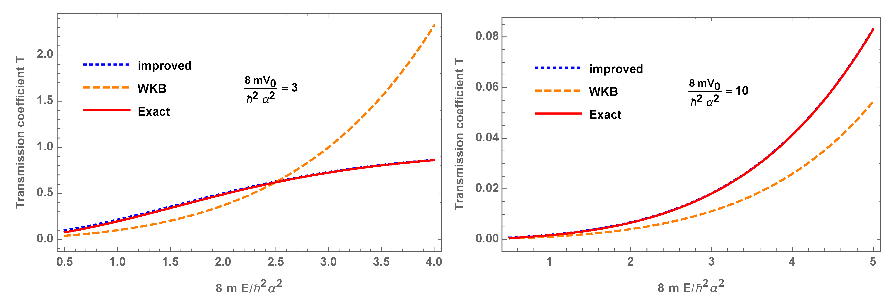
We first need to determine the choice of $q\left(x\right)$ to calculate the transmission coefficient (54) for a specific form of the potential. In this subsection, instead of calculating various potentials in details, let us consider the Pöschl-Teller potential barrier with a positive $v_0$ as an example. We note that this potential barrier has been applied to the calculation of the black hole quasi-normal modes [49,50] and the recent studying of the primordial perturbation during quantum bounce in the loop quantum cosmology [51,52,53,54]. The choice of $q\left(x\right)$ is the same as in the case for the Pöschl-Teller potential well. Subsequently, the transmission coefficient (54) reads

$$\begin{array}{c}\hfill T=\frac{1}{1+e^{\pi (\sqrt{8m{v}_0/{ħ}^2{\alpha }^2-1}-\sqrt{8mE/{ħ}^2{\alpha }^2})}},\end{array}$$

(55)

while the (standard) WKB approximation gives [55]

$$\begin{array}{c}\hfill T=e^{-\pi (\sqrt{8m{v}_0/{ħ}^2{\alpha }^2}-\sqrt{8mE/{ħ}^2{\alpha }^2})}.\end{array}$$

(56)

It is worth noting that the choice of $q\left(x\right)$ is only possible when $8m{v}_0/{ħ}^2>{\alpha }^2$ for positive $v_0$. When $8m{v}_0/{ħ}^2<{\alpha }^2$, as mentioned above, the choice of $q\left(x\right)$ changes the properties of turning points significantly, which makes the approximation not applicable. In Figure 1, we present the transmission coefficient (55), the WKB transmission coefficient (56), and the exact result, from which one can see that the transmission coefficient (55) fits the exact result extremely well.

4. Summary and Outlook

In this paper, a new analytical approximation method for solving the Schrödinger equation, the so-called uniform asymptotic approximation method, developed systematically by Olver [22,23], is presented and applied to several cases of interest in quantum mechanics. This new method makes use of the technique of uniform approximations to map the original Schrödinger equation to a simpler equation for which an approximate solution can be found analytically. One of the major advantage of the method is that the errors in each order of approximations can be estimated and their upper bounds are always known explicitly. In particular, for certain models, it was found that the errors are no larger than $0.15\%$ up to the third-order of approximations [36].

To illustrate the above, in this paper we have given the general solutions from the new method in the region where one single turning point or two turning points are encountered. One of the advantages of the new method is that, by carefully choosing the function $q\left(x\right)$, the errors of the approximate solutions can be well-controlled. In general, the function $q\left(x\right)$ has to be chosen to satisfy two conditions: (a) near the turning points $x_i$, $\left|q\left(x\right)\right|\ll |g\left(x\right)/(x-x_i)|$; and (b) away from the turning points, $\left|q\right(x\left)\right|\ll \left|g\right(x\left)\right|$. Moreover, when one of the the boundaries of the interesting region, for example $x=0$, becomes a second-order pole, $q\left(x\right)$ has to be fixed correspondingly to $-\frac{1}{4x^2}$ in order to make the error control function finite at the pole. One of the results from this particular choice of the function $q\left(x\right)$ is that the quantization conditions for bound states from the exact solutions can be recovered from our approximate solutions for several quantum mechanical systems. Moreover, when the form of the error control function can be analytically expressed in terms of $q\left(x\right)$ and $g\left(x\right)$, the function $q\left(x\right)$ can also be chosen to minimize the errors at the tuning point or at the extreme point. With the new method, we have also derived the transmission coefficients for particle scattering over a potential barrier, which significantly improve the accuracy of the results obtained from the standard WKB approximations.

It must be noted that in this article we have mainly compared the uniform asymptotic approximation method introduced in this paper with the conventional (standard) WKB approximations. Other methods, such as the complex [10,11,12,13,14] and uniform WKB [9,15,16,17,18], have also achieved great successes, and high (even exponential) precisions can be obtained. However, comparing the uniform asymptotic approximation method with them directly is not an easy task. In particular, the precisions of these methods, including the asymptotic approximation method, depend on the models and properties of the potentials $V\left(x\right)$ appearing in (1), and for a given model, one method might achieve much better precisions than others, but, in other models, the situation can be completely different. In the uniform WKB approximations and the current method, the analysis and precisions of a given problem also depend on the specific choice of the comparison equations [20,21,56]. When considering the scope of this paper, we shall leave this issue to another occasion.

The new analytical approximation method that is presented in this paper is also useful to future investigations on the high-order approximations, extension to the non-linear Schrödinger equation, and applications to various quantum systems with general potentials. Our formulas are general and simple to use, and they can also be applied to other interesting cases, for example, Hawking radiation and quasi-normal modes of black holes [49,50], primordial perturbations during inflation and reheating [57], and Schwinger vacuum pair productions due to laser pulses [58].

References

- Berry, M.V.; Mount, K.E. Semiclassical approximations in wave mechanics. Rep. Prog. Phys. 1972, 35, 315. [Google Scholar] [CrossRef] [Green Version]
- Friedrich, H.; Trost, J. Working with WKB waves far from the semiclassical limit. Phys. Rep. 2004, 397, 359. [Google Scholar] [CrossRef]
- Price, T.J.; Greene, C.H. Semiclassical Treatment of High-Lying Electronic States of . J. Phys. Chem. A 2018, 122, 8565. [Google Scholar] [CrossRef] [Green Version]
- Hyouguchi, T.; Adachi, S.; Ueda, M. Divergence-Free WKB Method. Phys. Rev. Lett. 2002, 88, 170404. [Google Scholar] [CrossRef] [PubMed] [Green Version]
- Karnakov, B.M.; Krainov, V.P. WKB Approximation in Atomic Physics; Springer: Berlin/Heidelberg, Germany, 2013. [Google Scholar]
- Fröman, N.; Fröman, P.O. JWKB Approximation: Contributions to the Theory; North Holland Publishing Company: Amsterdam, The Netherlands, 1965. [Google Scholar]
- Dong, S.-H. Wave Equations in Higher Dimensions; Springer: Dordrecht, The Netherlands; New York, NY, USA, 2011. [Google Scholar]
- Young, L.A.; Uhlenbeck, G.E. On the Wentzel-Brillouin-Kramers Approximate Solution of the Wave Equation. Phys. Rev. 1930, 36, 1154. [Google Scholar] [CrossRef]
- Langer, R.E. On the Connection Formulas and the Solutions of the Wave Equation. Phys. Rev. 1937, 51, 669. [Google Scholar] [CrossRef]
- Zwaan, A. Intensitäten im Ca Funkenspectrum. Ph.D. Thesis, Universiteitsbibliotheek Utrecht, Utrecht, The Netherlands, 1929. Available online: https://dspace.library.uu.nl/handle/1874/294713 (accessed on 30 June 2020).
- Langer, R. The Asymptotic Solutions of Linear Ordinary Differential Equations with Reference to the Stokes Phenomenon. Bull. Am. Math. Soc. 1934, 40, 545–582. [Google Scholar] [CrossRef] [Green Version]
- Landau, L.D.; Lifshitz, E.M. Quantum Mechanics (Non-Relativistic Theory), 3rd ed.; Butterworth-Heinemann: Beijing, China, 1997; pp. 46–53. [Google Scholar]
- Berry, M.V. Waves near Stokes lines. Proc. R. Soc. Lond. A 1990, 427, 265–280. [Google Scholar]
- Delabaere, E.; Dillinger, H.; Pham, F. Exact semiclassical expansions for one-dimensional quantum oscillators. J. Math. Phys. 1997, 38, 6126. [Google Scholar] [CrossRef] [Green Version]
- Miller, S.G.; Good, R.H. A WKB Type Approximation to the Schroedinger Equation. Phys. Rev. 1953, 91, 174–179. [Google Scholar] [CrossRef]
- Dingle, R.B. The method of comparison equations in the solution of linear second-order differential equations (generalized W.K.B. method). Appl. Sci. Res. B 1956, 5, 345. [Google Scholar] [CrossRef]
- Álvarez, G. Langer-Cherry derivation of the multi-instanton expansion for the symmetric double well. J. Math. Phys. 2004, 45, 3095. [Google Scholar] [CrossRef]
- Dunne, G.V.; Ünsal, M. Uniform WKB, multi-instantons, and resurgent trans-series. Phys. Rev. D 2014, 89, 105009. [Google Scholar] [CrossRef] [Green Version]
- Zinn-Justin, J. Quantum Field Theory and Critical Phenomena; Clarendon: Oxford, UK; New York, NY, USA, 2002. [Google Scholar]
- Slavyanov, S.Y. Asymptotic Solutions of the One-Dimensional Schrödinger Equation; American Mathematical Society: Providence, RI, USA, 1996. [Google Scholar]
- Fröman, N.; Fröman, P.O. Phase-Integral Method; Springer: New York, NY, USA, 1996. [Google Scholar]
- Olver, F.W.J. Second-Order Linear Differential Equations with Two Turning Points. Philos. Trans. R. Soc. Math. Phys. Eng. Sci. 1975, 278, 137. [Google Scholar]
- Olver, F.W.J. Asymptotics and Special Functions; A K Peters, Ltd.: Wellesley, MA, USA, 1997. [Google Scholar]
- Habib, S.; Heitmann, K.; Jungman, G.; Molina-Paris, C. The Inflationary perturbation spectrum. Phys. Rev. Lett. 2002, 89, 281301. [Google Scholar] [CrossRef] [Green Version]
- Habib, S.; Heinen, A.; Heitmann, K.; Jungman, G.; Molina-Paris, C. Characterizing inflationary perturbations: The Uniform approximation. Phys. Rev. D 2004, 70, 083507. [Google Scholar] [CrossRef] [Green Version]
- Wang, A. Vector and tensor perturbations in Horava-Lifshitz cosmology. Phys. Rev. 2010, 82, 124063. [Google Scholar] [CrossRef] [Green Version]
- Zhu, T.; Wang, A.; Cleaver, G.; Kirsten, K.; Sheng, Q. Power spectra and spectral indices of k-inflation: High-order corrections. Phys. Rev. D 2014, 90, 103517. [Google Scholar] [CrossRef] [Green Version]
- Alinea, A.L.; Kubota, T.; Naylor, W. Logarithmic divergences in the k-inflationary power spectra computed through the uniform approximation. J. Cosmol. Astropart. Phys. 2016, 2, 028. [Google Scholar] [CrossRef] [Green Version]
- Wu, Q.; Zhu, T.; Wang, A. Primordial Spectra of slow-roll inflation at second-order with the Gauss-Bonnet correction. Phys. Rev. D 2018, 97, 103502. [Google Scholar] [CrossRef] [Green Version]
- Alinea, A.L.; Kubota, T.; Nakanishi, Y.; Naylor, W. Adiabatic regularisation of power spectra in k-inflation. JCAP 2015, 6, 019. [Google Scholar] [CrossRef] [Green Version]
- Alinea, A.L. Adiabatic regularization of power spectra in nonminimally coupled chaotic inflation. J. Cosmol. Astropart. Phys. 2016, 10, 02. [Google Scholar] [CrossRef] [Green Version]
- Zhu, T.; Wang, A.; Cleaver, G.; Kirsten, K.; Sheng, Q. Constructing analytical solutions of linear perturbations of inflation with modified dispersion relations. Int. J. Mod. Phys. A 2014, 29, 1450142. [Google Scholar] [CrossRef] [Green Version]
- Zhu, T.; Wang, A.; Cleaver, G.; Kirsten, K.; Sheng, Q. Inflationary cosmology with nonlinear dispersion relations. Phys. Rev. D 2014, 89, 043507. [Google Scholar] [CrossRef] [Green Version]
- Zhu, T.; Wang, A. Gravitational quantum effects in light of BICEP2 results. Phys. Rev. D 2014, 90, 027304. [Google Scholar] [CrossRef] [Green Version]
- Zhu, T.; Wang, A.; Cleaver, G.; Kirsten, K.; Sheng, Q. Gravitational quantum effects on power spectra and spectral indices with higher-order corrections. Phys. Rev. D 2014, 90, 063503. [Google Scholar] [CrossRef] [Green Version]
- Zhu, T.; Wang, A.; Kirsten, K.; Cleaver, G.; Sheng, Q. High-order Primordial Perturbations with Quantum Gravitational Effects. Phys. Rev. D 2016, 93, 123525. [Google Scholar] [CrossRef] [Green Version]
- Qiao, J.; Ding, G.H.; Wu, Q.; Zhu, T.; Wang, A. Inflationary perturbation spectrum in extended effective field theory of inflation. J. Cosmol. Astropart. Phys. 2019, 1909, 064. [Google Scholar] [CrossRef] [Green Version]
- Ding, G.H.; Qiao, J.; Wu, Q.; Zhu, T.; Wang, A. Inflationary perturbation spectra at next-to-leading slow-roll order in effective field theory of inflation. Eur. Phys. J. C 2020, 101, 043528. [Google Scholar] [CrossRef]
- Qiao, J.; Zhu, T.; Zhao, W.; Wang, A. Polarized primordial gravitational waves in the ghost-free parity-violating gravity. Phys. Rev. D 2019, 79, 976. [Google Scholar] [CrossRef] [Green Version]
- Zhu, T.; Wang, A.; Kirsten, K.; Cleaver, G.; Sheng, Q.; Wu, Q. Inflationary spectra with inverse-volume corrections in loop quantum cosmology and their observational constraints from Planck 2015 data. J. Cosmol. Astropart. Phys. 2016, 1603, 046. [Google Scholar] [CrossRef] [Green Version]
- Zhu, T.; Wang, A.; Cleaver, G.; Kirsten, K.; Sheng, Q.; Wu, Q. Scalar and tensor perturbations in loop quantum cosmology: High-order corrections. J. Cosmol. Astropart. Phys. 2015, 1510, 052. [Google Scholar] [CrossRef] [Green Version]
- Zhu, T.; Wang, A.; Cleaver, G.; Kirsten, K.; Sheng, Q.; Wu, Q. Detecting quantum gravitational effects of loop quantum cosmology in the early universe? Astrophys. J. 2015, 807, L17. [Google Scholar] [CrossRef] [Green Version]
- Li, B.F.; Zhu, T.; Wang, A.; Kirsten, K.; Cleaver, G.; Sheng, Q. Pre-inflationary perturbations from deformed algebra approach in loop quantum cosmology. Phys. Rev. D 2019, 99, 103536. [Google Scholar] [CrossRef] [Green Version]
- Zhu, T.; Wu, Q.; Wang, A. An analytical approach to the field amplification and particle production by parametric resonance during inflation and reheating. Phys. Dark Univ. 2019, 26, 100373. [Google Scholar] [CrossRef] [Green Version]
- Miller, W.H. Classical S Matrix: Numerical Application to Inelastic Collisions. J. Chem. Phys. 1970, 53, 3578. [Google Scholar] [CrossRef]
- Cooper, F.; Khare, A.; Sukhatme, U.P. Supersymmetry in Quantum Mechanics; World Scientific: River Edge, NJ, USA; Singapore, 2001. [Google Scholar]
- Qiang, W.-C.; Dong, S.-H. Proper quantization rule. Europhys. Lett. 2010, 89, 10003. [Google Scholar] [CrossRef]
- Serrano, F.A.; Gu, X.-Y.; Dong, S.-H. Qiang-Dong proper quantization rule and its applications to exactly solvable quantum systems. J. Math. Phys. 2010, 51, 082103. [Google Scholar] [CrossRef]
- Konoplya, R.A.; Zhidenko, A. Quasinormal modes of black holes: From astrophysics to string theory. Rev. Mod. Phys. 2011, 83, 793. [Google Scholar] [CrossRef] [Green Version]
- Berti, E.; Cardoso, V.; Starinets, A.O. Quasinormal modes of black holes and black branes. Class. Quantum Gravity 2009, 26, 163001. [Google Scholar] [CrossRef]
- Wu, Q.; Zhu, T.; Wang, A. Nonadiabatic evolution of primordial perturbations and non-Gaussinity in hybrid approach of loop quantum cosmology. Phys. Rev. D 2018, 98, 103528. [Google Scholar] [CrossRef] [Green Version]
- Zhu, T.; Wang, A.; Kirsten, K.; Cleaver, G.; Sheng, Q. Primordial non-Gaussianity and power asymmetry with quantum gravitational effects in loop quantum cosmology. Phys. Rev. D 2018, 97, 043501. [Google Scholar] [CrossRef] [Green Version]
- Zhu, T.; Wang, A.; Cleaver, G.; Kirsten, K.; Sheng, Q. Pre-inflationary universe in loop quantum cosmology. Phys. Rev. D 2017, 96, 083520. [Google Scholar] [CrossRef] [Green Version]
- Zhu, T.; Wang, A.; Kirsten, K.; Cleaver, G.; Sheng, Q. Universal features of quantum bounce in loop quantum cosmology. Phys. Lett. B 2017, 773, 196. [Google Scholar] [CrossRef]
- Gottfried, K.; Yan, T.-M. Quantum Mechanics: Fundamentals, 2nd ed.; Springer: New York, NY, USA, 2003. [Google Scholar]
- Rosen, M.; Yennie, D.R. A Modified WKB Approximation for Phase Shifts. J. Math. Phys. 1964, 5, 1505. [Google Scholar] [CrossRef]
- Bassett, B.A.; Tsujikawa, S.; Wands, D. Inflation dynamics and reheating. Rev. Mod. Phys. 2006, 78, 537. [Google Scholar] [CrossRef] [Green Version]
- Dumlu, C.K.; Dunne, G.V. Stokes Phenomenon and Schwinger Vacuum Pair Production in Time-Dependent Laser Pulses. Phys. Rev. Lett. 2010, 104, 250402. [Google Scholar] [CrossRef] [Green Version]