
Holocene Millennial-Scale Solar Variability and the Climatic Responses on Earth


1
State Key Laboratory of Space Weather, National Space Science Center, Chinese Academy of Sciences, Beijing 100190, China
2
Yading Space Weather Science Center, Daocheng 627750, Ganzi, Sichuan, China
3
University of Chinese Academy of Sciences, Beijing 100049, China
4
CAS Key Laboratory of Solar Activity, National Astronomical Observatories, Beijing 100101, China
5
Center for Environmental Research and Earth Sciences (CERES), Salem, MA 01970, USA
6
Instituto de Geofísica, Universidad Nacional Autónoma de México, Circuito Exterior, C.U., Coyoacán, Mexico City 04510, Mexico
*
Author to whom correspondence should be addressed.
Universe 2021, 7(2), 36; https://0-doi-org.brum.beds.ac.uk/10.3390/universe7020036
Submission received: 31 December 2020
/
Revised: 29 January 2021
/
Accepted: 1 February 2021
/
Published: 4 February 2021
(This article belongs to the Special Issue Space Weather)
Abstract
:The solar impact on Earth’s climate is both a rich and open-ended topic with intense debates. In this study, we use the reconstructed data available to investigate periodicities of solar variability (i.e., variations of sunspot numbers) and temperature changes (10 sites spread all over the Earth) as well as the statistical inter-relations between them on the millennial scale during the past 8640 years (BC 6755–AD 1885) before the modern industrial era. We find that the variations of the Earth’s temperatures show evidence for the Eddy cycle component, i.e., the 1000-year cyclicity, which was discovered in variations of sunspot numbers and believed to be an intrinsic periodicity of solar variability. Further wavelet time-frequency analysis demonstrates that the co-variation between the millennium cycle components of solar variability and the temperature change held stable and statistically strong for five out of these 10 sites during our study interval. In addition, the Earth’s climatic response to solar forcing could be different region-by-region, and the temperatures in the southern hemisphere seemed to have an opposite changing trend compared to those in the northern hemisphere on this millennial scale. These findings reveal not only a pronounced but also a complex relationship between solar variability and climatic change on Earth on the millennial timescale. More data are needed to further verify these preliminary results in the future.
1. Introduction
The question of how strongly the Sun influences climate change on Earth is eternally debated, with topics ranging from the lack of evidence to contradictions. The debate involves another bigger and hotter topic, i.e., global warming, in the modern industrial period. It has been concluded that human influence, via emissions of greenhouse gases, is likely the dominant cause of the observed warming since the mid-20th century [1]. Yet it is equally clear that natural forces are still a non-negligible factor in driving climate change [2], involving co-modulating factors from both the intrinsic changes in solar irradiance and the Sun–Earth orbital conditions [3]. For example, the Earth’s planetary temperature experienced some periods in recent history that were probably as warm as the present, such as the Medieval Warm Period (AD 800–AD 1300), and other periods colder than present, such as the Little Ice Age (AD 1300–AD 1850). This proves that natural forces can drive climate change of large amplitude even without a powerful human influence. Solar forcing is one important ingredient of these natural driving factors [4,5,6]. Early in 1801, Sir William Herschel found that the rainfall reduced when there were few sunspots on the Sun, and pointed out that solar variability might play a role in the change of Earth’s climate [7,8]. The Maunder Minimum of anomalously low and weak sunspot activity (AD 1645–AD 1715) coincided in time with the coldest period of the Little Ice Age in many places of the world [9,10], as well as with that of the historical Ming-Qing Little Ice Age in China [11,12].
Sunspot number (SSN) is the most widely used parameter to qualitatively represent the timing and strength of solar magnetic activity, and this unique solar index also has the longest record time. Direct observations of sunspots started from the invention of the astronomical telescope, and, so far, scientists have accumulated only 400 years of data [13]. The available observational data would be insufficient in investigations exceeding centennial scales, such as millennial or even longer timescales. Fortunately, the proxy reconstructed data can be a reasonable substitute. Similarly, temperature is the most fundamental climatic index with long recording while the available instrumental thermometer data would be limited to studies of short timescales. There are many recent Holocene data sets reconstructed from various paleoclimatic proxies so far that have better resolution and chronology than earlier works [14]. For example, Marcott et al. [15] provided a wider view by reconstructing both regional and global temperatures for the past 11,300 years from 73 globally distributed sites. We found some clues about the evidence of solar modulation on the Earth’s climate change on a millennial scale in our last work [16], but the adopted climatic indicators were limited only to four local places on Earth (i.e., Greenland, Lake Qinghai and Dongge cave in China, Vostok in Antarctica). In this paper, we will explore the relations between solar variability and temperature changes for a more widely distributed database on Earth in order to check and expand our previous conclusions. This is an expanded follow-up of our last work [16].
2. Materials and Methods
The reconstructions of SSN are usually based on individual, sometimes statistically averaged, proxy data sets. Different from these, Wu et al. [17] combined the long-span data sets of 10Be and 14C in the available terrestrial archives to reconstruct, for the first time, a new consistent SSN data set. It covers 8640 years in the past (from BC 6755 to AD 1885) with the fixed time resolution of 10 years. We obtained this SSN data from their website (http://www2.mps.mpg.de/projects/sun-climate/data/SN_composite.txt).
For these 73 globally distributed temperature records used in Marcott et al. [16], we selected data for our analysis based on the following criteria: (1) covering the period BC 6755–AD 1885; (2) the time resolution higher than or about 100 years; (3) temperature coming from a single site, not composite ones. In this way we obtained temperature data of 10 sites (T1~T10) distributed from the Arctic to the Antarctic, i.e., temperatures of Agassiz-Renland, Tsuolbmajavri Lake, RAPID-12-1K, OCE326-GGC30, MD98-2181, ODP_1084B, TN057-17, Homestead Scarp, Dome C, and Vostok.
The reconstructed temperature of Agassiz-Renland (T1) was based on an average of uplift corrected δ18O data in the ice sheet from Agassiz and Renland [18]. The July temperature of Tsuolbmajavri Lake (T2) was reconstructed from pollen assemblages preserved in a sediment core [19]. The reconstruction of temperature of the Atlantic inflow RAPID-12-1K (T3) was based on paired Mg/Ca-δ18O measurements based on two species of planktonic foraminifera, Globigerina bulloides and Globorotalia inflata [20]. The alkenone-derived sea surface temperature (SST) of the slope water core OCE326-GGC30 (margin east of Nova Scotia basin, T4) was determined by alkenone paleothermometry [21]. The sea temperature of the marine sediment core MD98-2181 from the Morotai Basin (T5) was obtained from planktonic foraminiferal stable isotope and Mg/Ca records in the core [22].
The Mg/Ca data from ODP_1084B (Ocean Drilling Program Leg 175 Hole 1084B) in the Benguela coastal upwelling system recorded the oceanic temperature (T6) [23]. The summer SST at site TN057-17 near the Polar Front in the East Atlantic Southern Ocean (T7) was obtained from the down-core variability of diatom assemblages [24]. The summer temperature in the low forest at Homestead Scarp (T8) (in Campbell Island in the Southern Ocean) was reconstructed from the pollen peat sequence at temperature-sensitive locations within the tree-line ecotone [25]. The temperature in the European Project for Ice Coring in Antarctica Dome C ice core (T9) was obtained from a high-resolution deuterium profile in the core together with experiments performed with an atmospheric general circulation model including water isotopes [26]. Similarly, a data series of the local temperature at Vostok in East Antarctica (T10) was reconstructed for the past 420,000 years based on the deuterium content of the ice (δDice) in Vostok’s ice cores [27].
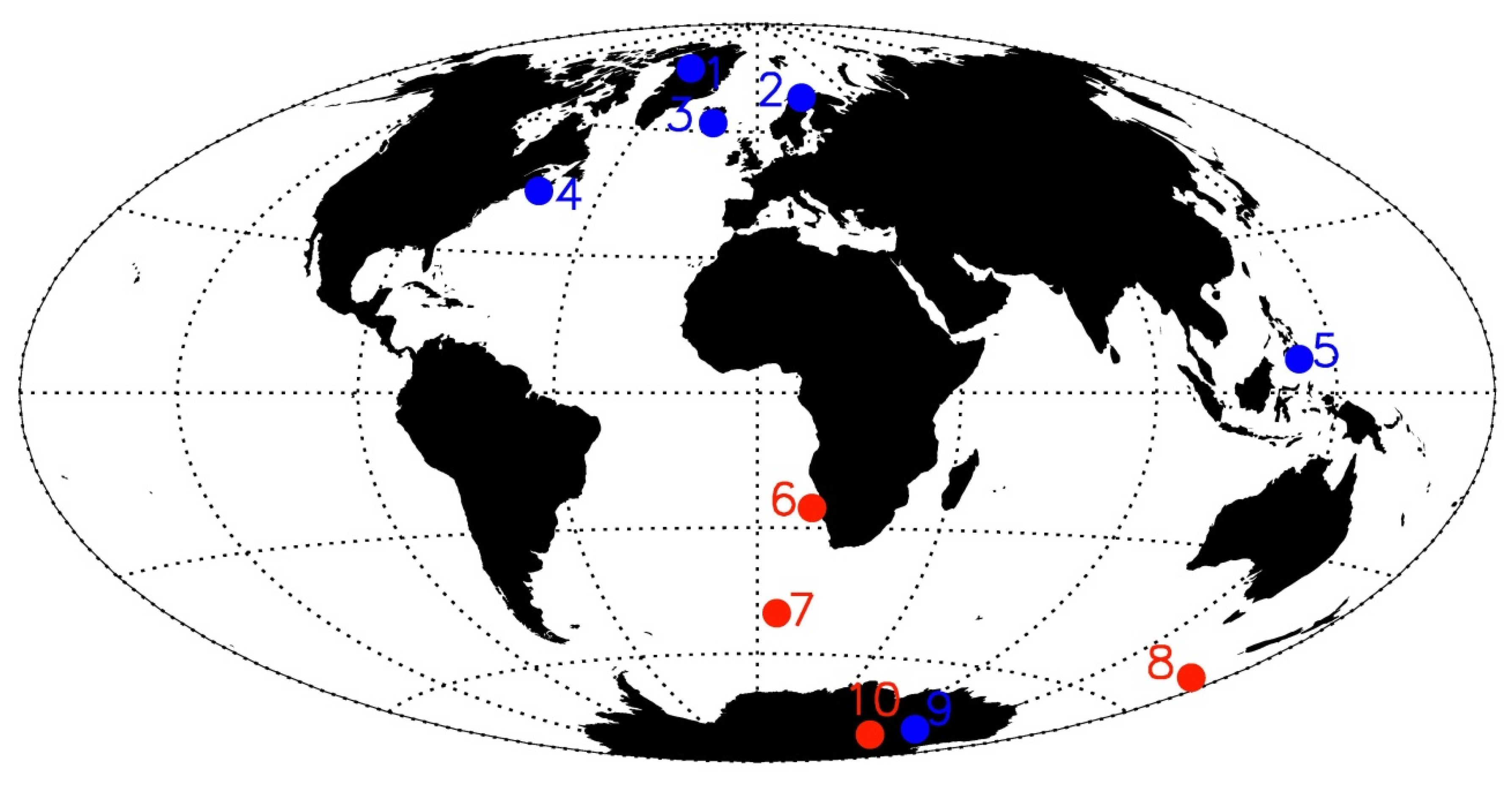
The reconstruction mechanisms and paleo-source media are greatly different for these 10 temperatures. Detailed information can be found in the related references, i.e., [18,19,20,21,22,23,24,25,26,27]. Table 1 lists the geographic information for their sites. Their locations on the Earth’s surface are shown in Figure 1. We can see that these 10 sites are evenly distributed in the northern and southern hemispheres, i.e., four sites located in the northern hemisphere (T1, T2, T3, T4), four sites in the southern hemisphere (T7, T8, T9, T10), and two sites in the tropical region on opposite sides of the equator (T5, T6), with similar latitudinal intervals between two neighboring sites. The averaged time resolution of each temperature is also given in Table 1. In order to align with SSN data, we computed the interpolations of T1~T10 from BC 6755 to AD 1885 at fixed time resolutions of 10 years, and adopted them as the temperature data.
We adopted the same analytical methods as those in our previous work [16]. We used the Lomb–Scargle periodogram method [28,29] to analyze periodicities of both solar variability and temperature change on Earth. This method has been widely used in geophysical research. In comparison with the traditional Fourier transform, this method had an evident advantage of applicability to incomplete or unevenly sampled time series.
In order to further disclose potential relations between solar variability and temperature change on Earth, we used the Wavelet Coherence (WTC) tool [30] to compute the wavelet coherence between SSN and temperatures. This wavelet coherence shows correlations of two signals in the time-frequency space and can display their relative phases, as well. Here, “frequency” can be converted to period (p) of the signal. Therefore, the corresponding wavelet coherence is expressed in the time-period space. We downloaded the software package of this tool from: http://noc.ac.uk/marine-data-products/cross-wavelet-wavelet-coherence-toolbox-matlab.
3. Results
3.1. Existence of the Millennial Cycle
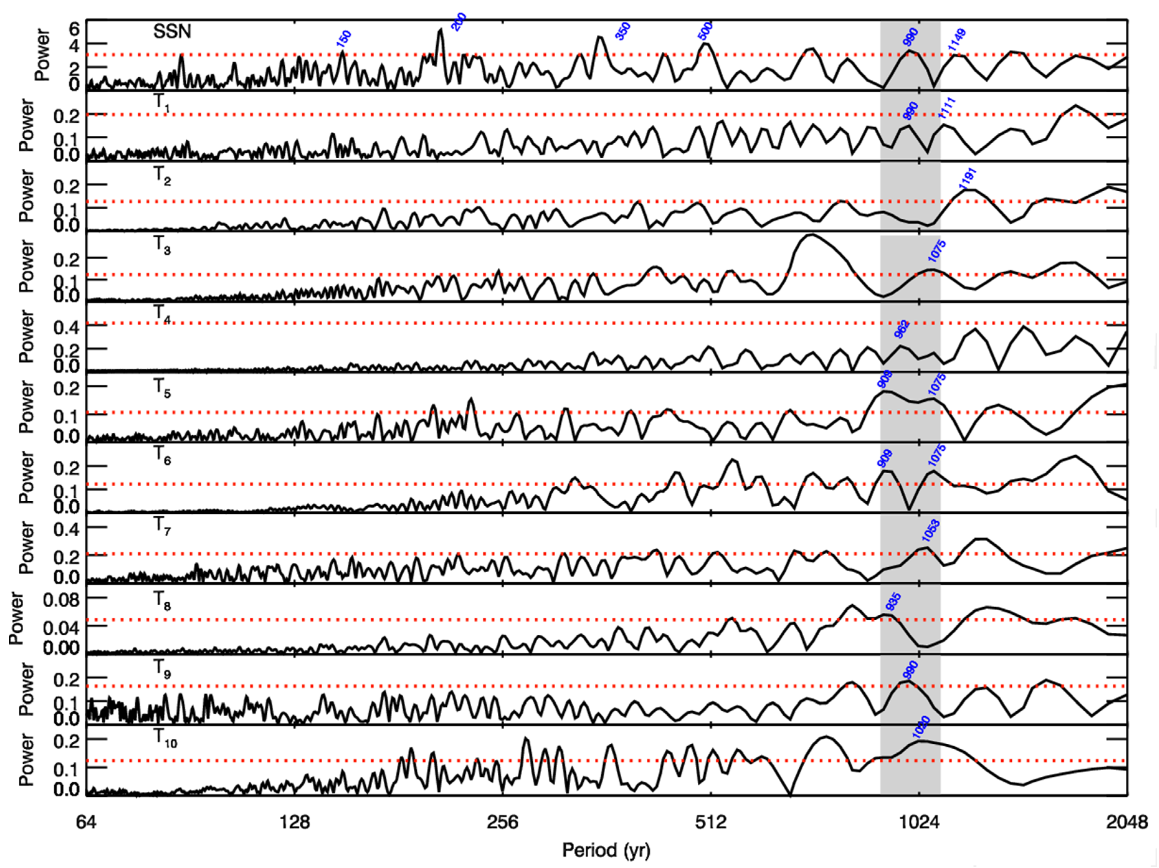
Figure 2 shows the Lomb–Scargle periodograms of these time series (both SSN and temperatures). The red horizontal dotted lines are the 95% confidence levels. We see that solar variability represented by SSN had a host of periodicities over the 95% confidence level, such as the 150-year cyclicity, 200-year cyclicity (Suess–de Vries cycle [31]), 350-year cyclicity, 500-year cyclicity, millennial cyclicity (990 years and 1149 years) (Eddy cycle [9,32,33,34]). Similar results were found in our previous study [16]. On the other hand, the temperatures had relatively fewer significant periodicities. The only common cyclicity between SSN and these temperatures was the Eddy cycle, which varied from 900 years to 1100 years (shaded region in Figure 2). For SSN, T5 and T6, there were two peaks over the 95% confidence level around the Eddy cycle; for other temperatures, only one peak was significant except for T4 (its peak at 962 years was lower than the 95% confidence level). The common periodicity between SSN and temperatures indicated potential physical connections, and attracted us to make further exploration between them.
3.2. Cross Correlations at Millennial Cycle
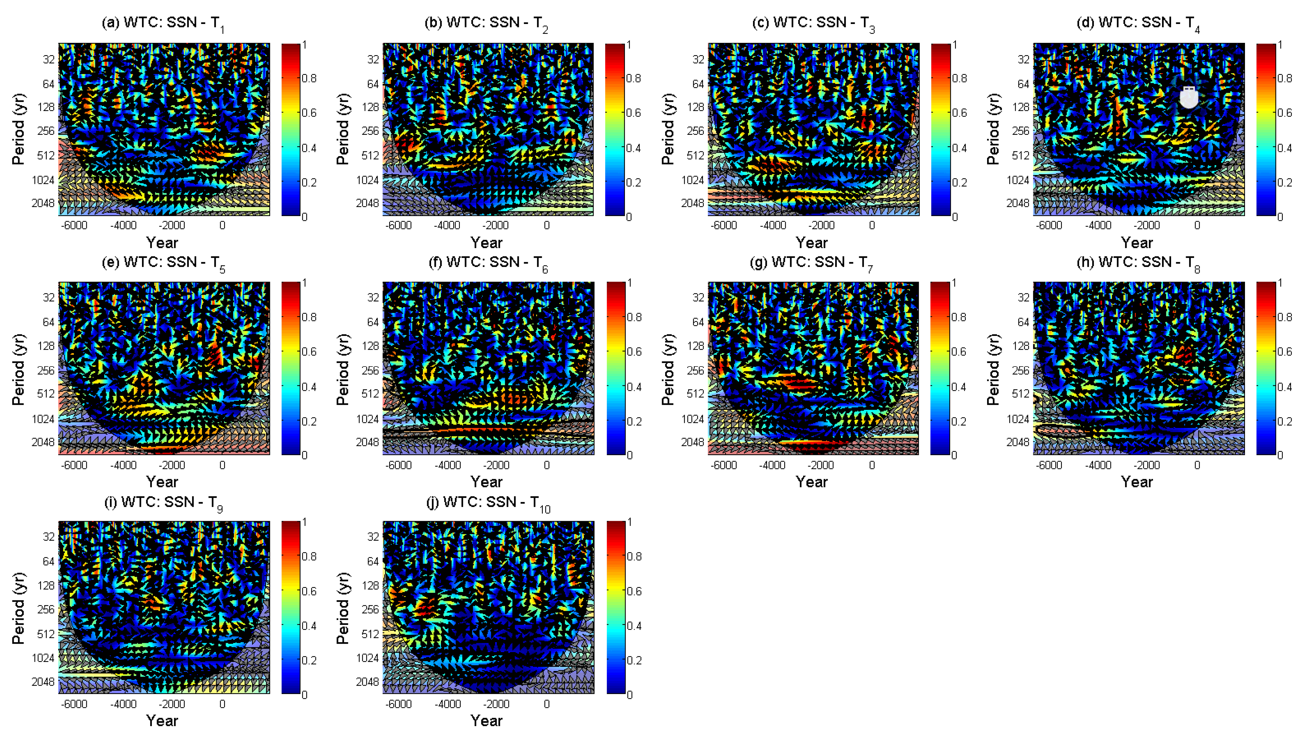
In order to further disclose potential relations between solar variability and temperature change on Earth, we used the Wavelet Coherence (WTC) tool [30] to compute the wavelet coherence between SSN and temperatures. Figure 3 gives the squared wavelet coherence (Cw) between SSN and T1, T2, …, T10, respectively. The definition of Cw can be found in Equation (8) of [30]. Most high-correlation regions appear as “isolated islands”, except for the high-power region around the millennium cycle. SSN had a good correlation to temperatures at this millennial cycle. The wavelet coherences at 1000-year cyclicity were stronger for T3, T4, T5 and T6 than those for the temperatures at other locations.
We adopted the global wavelet coherence Cg(p) and angle strength Sθ(p) to quantitatively estimate the cross-wavelet correlations between SSN and temperatures. They are parameters integrated along time at fixed period (p) in the wavelet coherence output by the WTC tool, and their detailed definitions can be found in [16]. Here, Cg reflects an overall correlation between two series at a fixed p, and Sθ depicts how strongly the phase angles between series keep stable. Cg = 1 means absolute correlation, and Cg = 0 means absolute non-correlation; Sθ = 1 indicates absolute “phase-locked”, and Sθ = 0 indicates absolute “non-phase-locked.” The combination of Cg and Sθ can reveal whether the co-variances of two analyzed series are strong and stable.
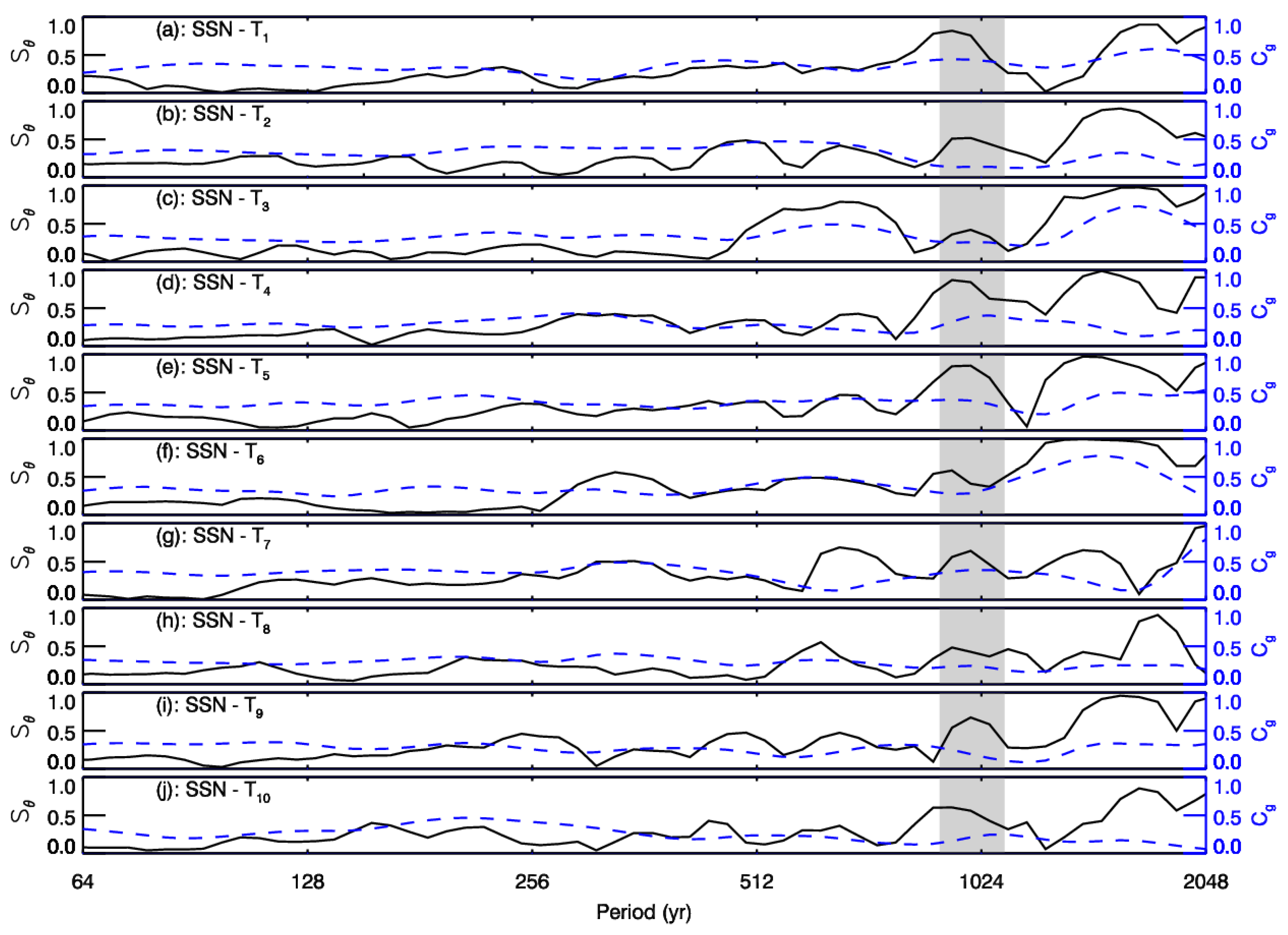
Figure 4 shows the variations of Cg and Sθ between SSN and temperatures along p outside the COI (cone of influence). The vertical shaded region denotes the millennial cyclicity, i.e., 900 years to 1100 years. We can see that both curves (Cg and Sθ) have peaks almost simultaneously at the millennial periodicity for T1, T4, T5, T7 and T10. For example, Sθ,peak(1ky) = 0.76 and Cg,peak(1ky) = 0.44 for T1. For the other temperatures (T2, T3, T6, T8, T9), their angle strengths present a peak at this millennial cycle, but the peak of their wavelet coherence is not so evident as those in angle strengths, meaning that only phases were securely locked at this millennial cycle. In general, this figure demonstrates that the wavelet coherences between SSN and temperatures kept strong and stable at the 1000-year cyclicity, relative to other cyclicities.
3.3. Solar Oscillations and Climatic Responses at Millennial Scale
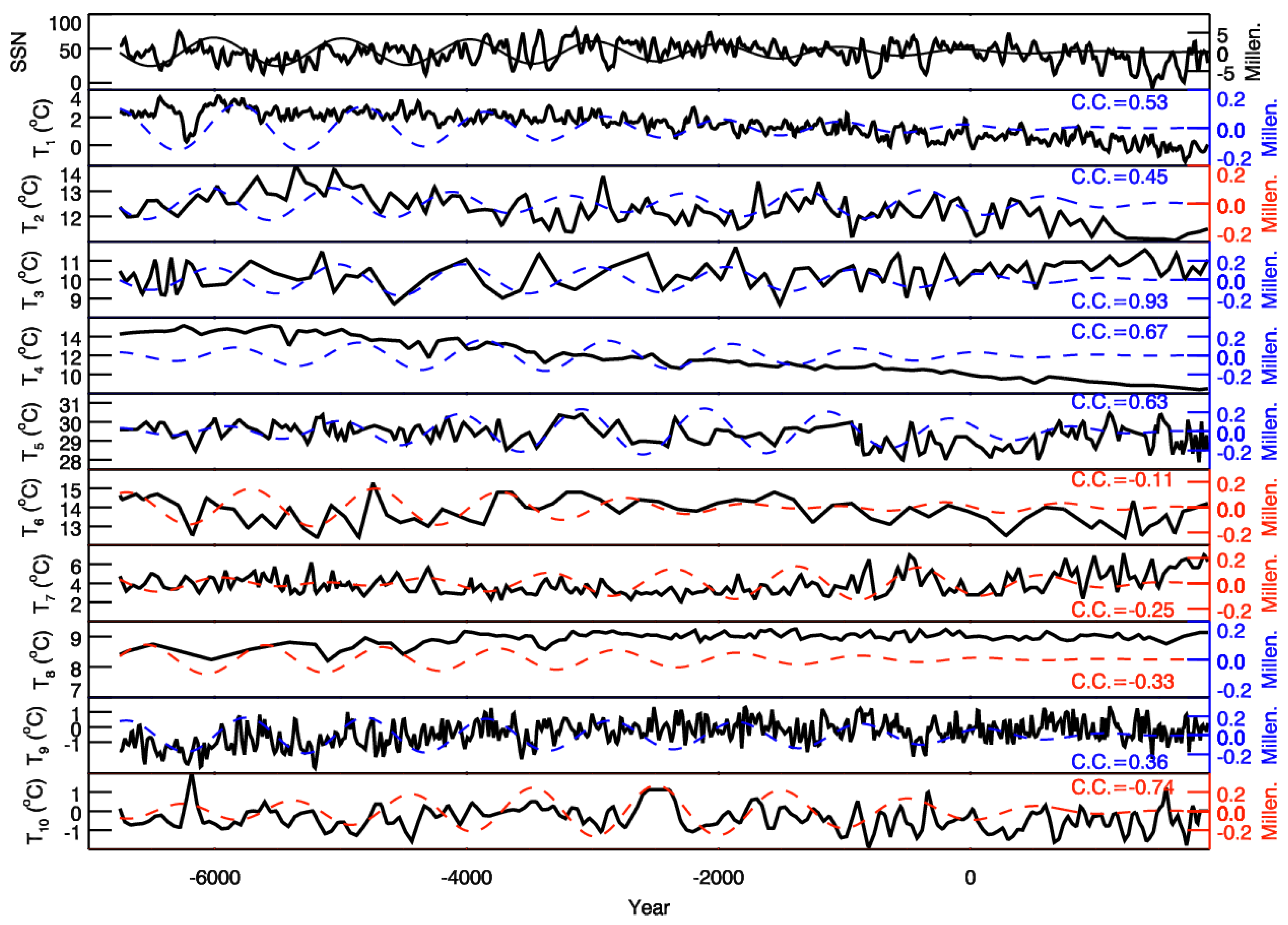
For a better display of the millennial evolutions of solar variability and climate changes on Earth, we used a band-pass filter to extract millennial signals from original data. The filter was designed to be centered at 1000 years, and its two half-power points were at 1000 ± 100 years. The output signals are shown in Figure 5 (thin lines). The millennial variations of SSN had a consistent trend with those of T1, T2, T3, T4, T5, T9, and positive correlations existed between them. The linear Pearson correlation coefficients (CCs) between SSN and these temperatures ranged from 0.36 (T9) to 0.93 (T3) (see values listed in Table 1). As for T6, T7, T8, T10, their changing trends were converse to that of SSN with negative correlations; T10 had the strongest negative correlation to SSN (CC = −0.74); and T6 had the weakest negative correlations (CC = −0.11). We adopted the tool developed by Macias-Fauria et al. [35] to estimate the statistical significance of these CCs. In this tool, a combination of Monte Carlo iterations and time-series modeling in the frequency [36] or temporal domains [37] was adopted to estimate the significance of CC by comparing the correlation to the distribution of correlations between the second target series and the random-phase series, which had the same periodogram as the first target series [36]. The CCs and their significance levels (p) between SSN and temperatures are shown in Table 2 as well.
From Table 2, we find the following results for millennial variations of these series. Firstly, all temperatures in the northern hemisphere (T1~T5) were positively correlated with SSN. As to temperatures in the southern hemisphere (T6~T10), four of them were negatively correlated with SSN except for T9. The site location is marked as a blue dot in Figure 1 if the corresponding temperature was positively correlated with SSN, and marked as a red dot for the negatively correlated temperature. Secondly, we were careful to the check the significance of these correlations. The significance levels were classified into four kinds: For T3, p < 0.001, indicating the CC was very significant; for T4 and T10, 0.1 < p < 0.2, indicating that their CCs were relatively significant; for T1 and T5, 0.2 < p < 0.3, therefore, their CCs to SSN were only weakly significant. For the other temperatures (T2, T6, T7, T8, T9), p > 0.3 for their CCs; we declared that their correlations to SSN were not statistically significant. Figure 5 also provides a direct comparison between SSN and temperatures for their original data (thick lines). We can see that the millennial components we derived here reflected the rough trends of their raw data on the millennial scale. The common periodicity of 1000 years (revealed in Figure 2), the generally strong and stable resonant relationships between SSN and temperatures during this periodicity (revealed in Figure 3, Figure 4 and Figure 5) jointly indicated that solar variability may have played a role in the modulation of this millennial oscillation of the Earth’s climate change, but the climatic responses on Earth are not uniform and can be different from region to region.
As far as the regional effects of climate change are concerned, an oppositely changing trend between the millennial temperatures of two hemispheres was discovered for 20 years [38,39,40,41,42,43,44], which can be termed “northern–southern hemispheric seesaw”. Based on our results, all temperatures in the northern hemisphere were positively correlated with SSN (T1, T3, T4, T5) but at different significance levels. For temperatures in the southern hemisphere, four out of five were negatively correlated with SSN, but only one (T10) was significant. This indicated that temperatures in the southern hemisphere seemed to have an opposite trend in contrast with the northern hemisphere’s temperatures on the millennial scale. This was consistent with previous studies on seesaw [42,45]. For example, the modeling work demonstrated that responses of regional temperatures to the solar forcing were not uniform [42]; although the millennial variations of the northern temperature kept the positive-phase consistency with the global change, a small part of the very southern regions presented a converse trend with the global variation [45].
The seesaw pattern, also revealed by other evidences, seemed to be a robust feature of the long-term climate change on Earth [40,41]. For example, Eroglu et al. [46] found a seesaw variation in the Holocene East Asian–Australian summer monsoon at millennial to sub-centennial timescales during the past 9000 years. However, our results indicated a complex seesaw pattern of the Earth’s climatic responses to solar forcing, rather than a strict northern–southern seesaw: different regions within the same hemisphere could have different significant levels of variations, even an opposite changing trend. Although some regions presented evident responses to solar forcing, other regions might have been insensitive to the driving forcing. This further indicated that if we considered the region-averaged temperatures on Earth (especially for regions in the southern hemisphere), it would be difficult to uncover the potential seesaw relation between them as the averaging process would weaken the differences between regions. This fact might explain why this millennial seesaw pattern of the Earth’s climate was so highly controversial [47,48].
4. Conclusions and Discussion
In summary, we selected temperatures from 10 sites evenly distributed on the Earth’s surface with time resolutions higher than 100 years to probe periodicities and cross correlations between solar variability and local temperatures on Earth. Spectral analysis demonstrated that the millennial-scale cycle was the only common oscillation between SSN and all these local temperatures on Earth for our study interval (BC 6755–AD 1885). Further cross-wavelet analysis revealed that the millennial cycle components of SSN and temperatures had stable but varying values in the statistical correlations. These findings indicated that solar variability may have played a role in the modulation of this millennial variation of the Earth’s climate, but the spatial patterns of climatic responses on the Earth are complex. For the 10 temperature records on the Earth, six gave positive correlations to SSN (five in the northern hemisphere, and one in the southern hemisphere), four gave negative correlations to SSN (all in the southern hemisphere) on the millennial time scale. Here tropical regions were classified into northern/southern hemisphere strictly. But the correlations were only statistically significant for five temperatures (four in the northern hemisphere with all positive correlations, and one in the southern hemisphere with negative correlation).
The mechanisms to explain the results obtained here involved two aspects: the solar impact mechanism and the response mechanism of the Earth’s climate. For the former, the atmospheric general circulation models (GCMs) showed that when solar variability was low the changes in stratospheric ozone would trigger downward-propagating effects, which led to cooling in the high northern latitude atmosphere, a southward shift of the northern subtropical jet, and a decrease in the Northern Hadley circulation [4,49]. Bond et al. [50] pointed out that these atmospheric responses further led to an increase of the North Atlantic drift ice, cooling in Greenland, reduced monsoon activity, and reduced rainfall in low latitudes; then these atmospheric changes were amplified and transferred to other regions through their impacts on sea ice and North Atlantic thermohaline overturning [50,51,52]. Confirming the latter chain of mechanisms was far beyond the scope of this paper, but we still can list some useful clues here. The complicated oceanic circulation, especially that involving redistribution of heat through long-range advective transport, could lead to opposite trends of climate change in different regions on Earth [38,53]. We can speculate that solar variability first generates an overall positive feedback, like the atmospheric water vapor feedback [8], on the global Earth. Then this global change will lead to a negative feedback in local regions on Earth through complex oceanic and/or atmospheric processes. We note that results derived here are tentative and preliminary, and more observational evidences, rather than theoretical speculations, are needed in the next steps to generalize the findings, in addition to more credible physical mechanisms accounting for the complex responses of the Earth’s climate.
Author Contributions
X.Z. designed the research. X.Z., W.S., and V.M.V.H. participated in data analyses, interpretation, discussion, and writing of the manuscript. All authors have read and agreed to the published version of the manuscript.
Funding
This research was jointly supported by the Strategic Priority Research Program of Chinese Academy of Sciences (Grant No. XDB 41000000), the NSFC grants (41531073, 41731067, 41861164026, 41874202, 41474153), the Youth Innovation Promotion Association of Chinese Academy of Sciences (2016133), the collaborating research program (CRP) of CAS Key Laboratory of Solar Activity NAO, and Chinese Academy of Sciences Research Fund for Key Development Directions.
Acknowledgments
We acknowledge the use of the reconstructed SSN data from the research group “solar variability and climate” in MPS (http://www2.mps.mpg.de/projects/sun-climate/data/SN_composite.txt). We acknowledge the use of NOAA’s paleoclimatology data website (https://www.ncdc.noaa.gov/data-access/paleoclimatology-data) to download the reconstructed temperature data. We thank Janet M Wilmshurst at the University of Auckland for providing the temperature data of Homestead scarp.
Conflicts of Interest
The authors declare no conflict of interest.
References
- Stocker, V.B.; Qin, D.; Plattner, G.K.; Tignor, M.; Allen, S.K.; Boschung, J.; Nauels, A.; Xia, Y. Summary for policymakers. In Climate Change 2013: The Physical Science Basis. Contribution of Working Group I to the Fifth Assessment Report of the Intergovernmental Panel on Climate Change; University Press: Cambridge, UK; New York, NY, USA, 2013. [Google Scholar]
- Lüning, S.; Vahrenholt, F. The sun’s role in climate. In Evidence-Based Climate Science; Elsevier: Amsterdam, The Netherlands, 2016; Chapters 6; pp. 283–306. [Google Scholar]
- Cionco, R.G.; Soon, W. Short-term orbital forcing: A quasi-review and a reappraisal of realistic boundary conditions for climate modeling. Earth-Sci. Rev. 2017, 166, 206–222. [Google Scholar] [CrossRef] [Green Version]
- Haigh, J.D. The impact of solar variability on climate. Science 1996, 272, 981–985. [Google Scholar] [CrossRef]
- Gray, L.J.; Beer, J.; Geller, M.; Haigh, J.D.; Lockwood, M.; Matthes, K.; Cubasch, U.; Fleitmann, D.; Harrison, G.; Hood, L.; et al. Solar influences on climate. Rev. Geophys. 2010, 48. [Google Scholar] [CrossRef]
- Soon, W.; Connolly, R.; Connolly, M. Re-evaluating the role of solar variability on northern hemisphere temperature trends since the 19th century. Earth-Sci. Rev. 2015, 150, 409–452. [Google Scholar] [CrossRef]
- Herschel, W. Observations tending to investigate the nature of the sun, in order to find the causes or symptoms of its variable emission of light and heat: With remarks on the use that may possibly be drawn from solar observations. Philos. Trans. R. Soc. Lond. 1801, 91, 265–318. [Google Scholar]
- Soon, W.; Baliunas, S. A Brief Review of the Sun-Climate Connection, with a New Insight Concerning Water Vapour; Institute of Public Affairs: Melbourne, VIC, Australia, 2017. [Google Scholar]
- Eddy, J.A. The Maunder minimum. Science 1976, 192, 1189–1202. [Google Scholar] [CrossRef] [Green Version]
- Soon, W.; Yaskell, S.H. The Maunder Minimum and the Variable Sun-Earth Connection; World Scientific Pub Co Inc.: Singapore, 2003. [Google Scholar]
- Soon, W.; Baliunas, S.; Idso, C.; Idso, S.; Legates, D.R. Reconstructing climatic and environmental changes of the past 1000 years: A reappraisal. Energy Environ. 2003, 14, 233–296. [Google Scholar] [CrossRef]
- Xiao, J.; Zheng, G.Z.; Guo, Z.S.; Yan, L.S. Climate change and social response during the heyday of the little ice age in the Ming and Qing dynasties. J. Arid Land Resour. Environ. 2018, 32, 79–84. [Google Scholar]
- Clette, F.; Svalgaard, L.; Vaquero, J.M.; Cliver, E.W. Revisiting the sunspot number a 400-year perspective on the solar cycle. Spa. Sci. Rev. 2014, 186, 35–103. [Google Scholar] [CrossRef] [Green Version]
- Kaufman, D.S.; McKay, N.P.; Routson, C.; Erb, M.; Dätwyler, C.; Sommer, P.S.; Heiri, O.; Davis, B. Holocene global mean surface temperature, a multi-method reconstruction approach. Sci. Data 2020, 7, 1–13. [Google Scholar] [CrossRef]
- Marcott, S.A.; Shakun, J.D.; Clark, P.U.; Mix, A.C. A reconstruction of regional and global temperature for the past 11,300 years. Science 2013, 1198–1201. [Google Scholar] [CrossRef] [Green Version]
- Zhao, X.H.; Soon, W.; Velasco Herrera, V.M. Evidence for solar modulation on the millennial-scale climate change of Earth. Universe 2020, 6, 153. [Google Scholar] [CrossRef]
- Wu, C.-J.; Usoskin, I.G.; Krivova, N.; Kovaltsov, G.A.; Baroni, M.; Bard, E.; Solanki, S.K. Solar activity over nine millennia: A consistent multi-proxy reconstruction. Astron. Astrophys. 2018, 615, A93. [Google Scholar] [CrossRef] [Green Version]
- Vinther, B.M.; Buchardt, S.L.; Clausen, H.B.; Dahl-Jensen, D.; Johnsen, S.J.; Fisher, D.A.; Koerner, R.M.; Raynaud, D.; Lipenkov, V.; Andersen, K.K.; et al. Holocene thinning of the Greenland ice sheet. Nat. Cell Biol. 2009, 461, 385–388. [Google Scholar] [CrossRef]
- Seppä, H.; Birks, H.J.B. July mean temperature and annual precipitation trends during the Holocene in the Fennoscandian tree-line area: Pollen-based climate reconstructions. Holocene 2011, 11, 527–539. [Google Scholar] [CrossRef] [Green Version]
- Thornalley, D.J.R.; Elderfield, H.; McCave, I.N. Holocene oscillations in temperature and salinity of the surface subpolar North Atlantic. Nature 2009, 457, 711–714. [Google Scholar] [CrossRef] [PubMed]
- Sachs, J.P. Cooling of Northwest Atlantic slope waters during the Holocene. Geophys. Res. Lett. 2007, 34, L03609. [Google Scholar] [CrossRef] [Green Version]
- Stott, L.; Timmermann, A.; Thunell, R. Southern hemisphere and deep-sea warming led deglacial atmospheric CO2 rise and tropical warming. Science 2007, 318, 435–438. [Google Scholar] [CrossRef] [Green Version]
- Farmer, E.C.; de Menocal, P.B.; Marchitto, T.M. Holocene and deglacial ocean temperature variability in the Benguela upwelling region: Implications for low-latitude atmospheric circulation. Paleoceanography 2005, 20, PA2018. [Google Scholar] [CrossRef]
- Nielsen, S.H.H.; Koc, N.; Crosta, X. Holocene climate in the Atlantic sector of the Southern Ocean: Controlled by insolation or oceanic circulation? Geology 2004, 32, 317–320. [Google Scholar] [CrossRef]
- McGlone, M.S.; Turney, C.S.M.; Wilmshurst, J.M.; Renwich, J.; Pahnke, K. Divergent trends in land and ocean temperature in the Southern Ocean over the past 18,000 years. Nat. Geosci. 2010, 3, 622–626. [Google Scholar] [CrossRef]
- Jouzel, J.; Masson-Delmotte, V.; Cattani, O.; Dreyfus, G.; Falourd, S.; Hoffmann, G.; Minster, B.; Nouet, J.; Barnola, J.-M.; Chappellaz, J.; et al. Orbital and Millennial Antarctic Climate Variability over the Past 800,000 Years. Science 2007, 317, 793–796. [Google Scholar] [CrossRef] [Green Version]
- Petit, J.R.; Jouzel, J.; Raynaud, D.; Barkov, N.I.; Barnola, J.-M.; Basile-Doelsch, I.; Bender, M.L.; Chappellaz, J.; Davis, M.L.; Delaygue, G.; et al. Climate and atmospheric history of the past 420,000 years from the Vostok ice core, Antarctica. Nature 1999, 399, 429–436. [Google Scholar] [CrossRef] [Green Version]
- Lomb, N.R. Least-squares frequency analysis of unequally spaced data. Astrophys. Space Sci. 1976, 39, 447–462. [Google Scholar] [CrossRef]
- Scargle, J.D. Studies in astronomical time series analysis. II. Statistical aspects of spectral analysis of unevenly spaced data. Astrophys. J. 1982, 263, 835–853. [Google Scholar] [CrossRef]
- Grinsted, A.; Moore, J.C.; Jevrejeva, S. Application of the cross wavelet transform and wavelet coherence to geophysical time series. Nonlin. Process. Geophys. 2004, 11, 561–566. [Google Scholar] [CrossRef]
- Suess, H.E. The radio carbon record in tree rings of the last 8000 years. Radiocarbon 1980, 22, 200–209. [Google Scholar] [CrossRef] [Green Version]
- Abreu, J.A.; Beer, J.; Ferriz-Mas, A.; McCracken, K.G.; Steinhilber, F. Is there a planetary influence on solar activity? Astron. Astrophys. 2012, 584, A88. [Google Scholar] [CrossRef] [Green Version]
- McCracken, K.G.; Beer, J.; Steinhilber, F.; Abreu, J. A phenomenological study of the cosmic ray variations over the past 9400 years, and their implications regarding solar activity and the solar dynamo. Sol. Phys. 2013, 286, 609–627. [Google Scholar] [CrossRef]
- McCracken, K.G.; Beer, J.; Steinhilber, F. Evidence for planetary forcing of the cosmic ray intensity and solar activity throughout the past 9400 years. Sol. Phys. 2014, 289, 3207–3229. [Google Scholar] [CrossRef]
- Macias-Fauria, M.; Grinsted, A.; Helama, S.; Holopainen, J. Persistence matters: Estimation of the statistical significance of paleoclimatic reconstruction statistics from autocorrelated time series. Dendrochronologia 2012, 30, 179–187. [Google Scholar] [CrossRef]
- Ebisuzaki, W. A method to estimate the statistical significance of a correlation when the data are serially correlated. J. Clim. 1997, 10, 2147–2153. [Google Scholar] [CrossRef]
- Burg, J.P. A new analysis technique for time series data. In Modern Spectrum Analysis; Chiders, D.G., Ed.; IEEE Press: New York, NY, USA, 1978; pp. 42–48. [Google Scholar]
- Broecker, W.S. Paleocean circulation during the last deglaciation: A bipolar seesaw? Paleoceanography 1998, 13, 119–121. [Google Scholar] [CrossRef]
- Stocker, T.F. Past and future reorganizations in the climate system. Quat. Sci. Rev. 2000, 19, 301–319. [Google Scholar] [CrossRef]
- Blunier, T.; Brook, E.J. Timing of millennial-scale climate change in Antarctica and Greenland during the last glacial period. Science 2001, 291, 109–112. [Google Scholar] [CrossRef]
- Denton, G.H.; Broecker, W.S. Wobbly ocean conveyor circulation during the Holocene? Quat. Sci. Rev. 2008, 27, 1939–1950. [Google Scholar] [CrossRef]
- Swingedouw, D.; Terray, L.; Cassou, C.; Voldoire, A.; Salas-Mélia, D.; Servonnat, J. Natural forcing of climate during the last millennium: Fingerprint of solar activity. Clim. Dyn. 2011, 36, 1349–1364. [Google Scholar] [CrossRef]
- Rella, S.F.; Uchida, M. A Southern Ocean trigger for Northwest Pacific ventilation during the Holocene? Sci. Rep. 2014, 4, 4046. [Google Scholar] [CrossRef]
- Members, W.D.P. Precise interpolar phasing of abrupt climate change during the last ice age. Nature 2015, 520, 661–665. [Google Scholar] [CrossRef] [Green Version]
- Lüdecke, H.J.; Hempelmann, A.; Weiss, C.O. Multi-periodic climate dynamics: Spectral analysis of long-term instrumental and proxy temperature records. Clim. Past 2013, 9, 447–452. [Google Scholar] [CrossRef] [Green Version]
- Eroglu, D.; McRobie, F.H.; Ozken, I.; Stemler, T.; Wyrwoll, K.-H.; Breitenbach, S.F.M.; Marwan, N.; Kurths, J. See–saw relationship of the Holocene East Asian–Australian summer monsoon. Nat. Commun. 2016, 7, 12929. [Google Scholar] [CrossRef] [Green Version]
- Wunsch, C. Greenland–Antarctic phase relations and millennial time-scale climate fluctuations in the Greenland ice-cores. Quat. Sci. Rev. 2003, 22, 1631–1646. [Google Scholar] [CrossRef]
- Markle, B.R.; Steig, E.J.; Buizert, C.; Schoenemann, S.W.; Bitz, E.J.S.C.M.; Fudge, T.J.; Pedro, J.B.; Ding, Q.; Jones, T.R.; White, J.W.C.; et al. Global atmospheric teleconnections during Dansgaard–Oeschger events. Nat. Geosci. 2017, 10, 36–40. [Google Scholar] [CrossRef]
- Shindell, D.; Rind, D.; Balachandran, N.; Lean, J.; Lonergan, P. Solar cycle variability, ozone, and climate. Science 1999, 284, 305–308. [Google Scholar] [CrossRef] [Green Version]
- Bond, G.; Kromer, B.; Beer, J.; Muscheler, R.; Evans, M.N.; Showers, W.; Hoffmann, S.; Lotti-Bond, R.; Hajdas, I.; Bonani, G. Persistent Solar Influence on North Atlantic Climate During the Holocene. Science 2001, 294, 2130–2136. [Google Scholar] [CrossRef] [PubMed] [Green Version]
- Holland, M.; Bitz, C.M.; Eby, M.; Weaver, A.J. The role of ice-ocean interactions in the variability of the North Atlantic thermohaline circulation. J. Climate 2001, 14, 656–675. [Google Scholar] [CrossRef]
- Soon, W.W.-H. Solar Arctic-mediated climate variation on multidecadal to centennial timescales: Empirical evidence, mechanistic explanation, and testable consequences. Phys. Geogr. 2009, 30, 144–184. [Google Scholar] [CrossRef]
- Crowley, T.J. North Atlantic deep water cools the southern hemisphere. Paleoceanography 1992, 7, 489–497. [Google Scholar] [CrossRef]
Figure 1.
Locations of 10 sites of the reconstructed temperature data adopted in this study. Blue dots denote locations of temperatures with positive correlations to sunspot number (SSN) reported in Table 1 (see also Figure 5), and red dots denote those with negative correlations to SSN. A rough pattern of opposing inter-hemispheric seesaw temperature responses to solar variations on the millennial timescale over the Holocene, with the one exception of T9, is indicated.

Figure 2.
The Lomb–Scargle periodograms of SSN and 10 temperatures on Earth during the study interval (BC 7290–AD 1850). The red horizontal dotted lines denote the 95% confidence levels. The shaded region represents the Eddy cycle (roughly 900 years to 1100 years).
Figure 2.
The Lomb–Scargle periodograms of SSN and 10 temperatures on Earth during the study interval (BC 7290–AD 1850). The red horizontal dotted lines denote the 95% confidence levels. The shaded region represents the Eddy cycle (roughly 900 years to 1100 years).

Figure 3.
Cross-wavelet analyses between SSN and temperatures. The red regions enclosed by thick black lines denote their confidence levels higher than 95% against red noise. The light black curve denotes the “cone of influence” (COI).
Figure 3.
Cross-wavelet analyses between SSN and temperatures. The red regions enclosed by thick black lines denote their confidence levels higher than 95% against red noise. The light black curve denotes the “cone of influence” (COI).

Figure 4.
The phase angle strength (Sθ, solid line) and global wavelet coherence (Cg, blue dashed line) between SSN and temperatures plotted against period. The shaded region marks the millennial period (roughly 900 years to 1100 years).
Figure 4.
The phase angle strength (Sθ, solid line) and global wavelet coherence (Cg, blue dashed line) between SSN and temperatures plotted against period. The shaded region marks the millennial period (roughly 900 years to 1100 years).

Figure 5.
Comparison between SSN and temperatures (thick lines) and their 1000-year cycle components (thin lines). Blue lines represent temperatures positively correlated with SSN, while red lines represent temperatures negatively correlated with SSN. See text for results and discussion as well as summary in Table 1 and Table 2, and Figure 1.


Table 1.
Holocene temperatures of 10 sites used in this study and their (averaged) time resolutions.
Table 1.
Holocene temperatures of 10 sites used in this study and their (averaged) time resolutions.
| Site Name | Temperature | Latitude (°) | Longitude (°) | Elevation (m) | Time Resolution (yr) |
|---|---|---|---|---|---|
| Agassiz-Renland | T1 | 71.2/81.0 | −26.7/−71.0 | 1730/2350 | 20 |
| Tsuolbmajavri Lake | T2 | 68.7 | 22.1 | 526 | 67 |
| RAPID-12-1k | T3 | 62.1 | −17.8 | −1938 | 95 |
| OCE326-GGC30 | T4 | 44.0 | −63.0 | −250 | 79 |
| MD98-2181 | T5 | 6.3 | 125.8 | −2114 | 47 |
| ODP-1084B | T6 | −25.5 | 13.0 | −1992 | 117 |
| TN057-17 | T7 | −50.0 | 6.0 | −3700 | 43 |
| Homestead Scarp | T8 | −52.5 | 169.1 | 30 | 60 |
| Dome C | T9 | −75.1 | 123.4 | 3260 | 18 |
| Vostok | T10 | −78.5 | 108.0 | 3500 | 41 |
Table 2.
The correlation coefficient (CC) values and their significance levels (p) between SSN and 10 temperatures (T1~T10).
Table 2.
The correlation coefficient (CC) values and their significance levels (p) between SSN and 10 temperatures (T1~T10).
| T1 | T2 | T3 | T4 | T5 | T6 | T7 | T8 | T9 | T10 | |
|---|---|---|---|---|---|---|---|---|---|---|
| CC | 0.53 | 0.45 | 0.93 | 0.67 | 0.63 | −0.11 | −0.25 | −0.33 | 0.36 | −0.74 |
| p | 0.27 | >0.3 | <0.001 | 0.17 | 0.21 | >0.3 | >0.3 | >0.3 | >0.3 | 0.11 |
Publisher’s Note: MDPI stays neutral with regard to jurisdictional claims in published maps and institutional affiliations. |
© 2021 by the authors. Licensee MDPI, Basel, Switzerland. This article is an open access article distributed under the terms and conditions of the Creative Commons Attribution (CC BY) license (http://creativecommons.org/licenses/by/4.0/).
Share and Cite
MDPI and ACS Style
Zhao, X.; Soon, W.; Velasco Herrera, V.M. Holocene Millennial-Scale Solar Variability and the Climatic Responses on Earth. Universe 2021, 7, 36. https://0-doi-org.brum.beds.ac.uk/10.3390/universe7020036
AMA Style
Zhao X, Soon W, Velasco Herrera VM. Holocene Millennial-Scale Solar Variability and the Climatic Responses on Earth. Universe. 2021; 7(2):36. https://0-doi-org.brum.beds.ac.uk/10.3390/universe7020036
Chicago/Turabian StyleZhao, Xinhua, Willie Soon, and Victor M. Velasco Herrera. 2021. "Holocene Millennial-Scale Solar Variability and the Climatic Responses on Earth" Universe 7, no. 2: 36. https://0-doi-org.brum.beds.ac.uk/10.3390/universe7020036
Note that from the first issue of 2016, this journal uses article numbers instead of page numbers. See further details here.