Identification of Fractal Properties in Geomagnetic Data of Southeast Asian Region during Various Solar Activity Levels

Abstract

The fractal properties of geomagnetic northward component data (H-component) in the equatorial region during various phases of solar activity over Southeast Asia were investigated and then quantified using the parameter of the Hurst exponent (H). This study began with the identification of existence of spectral peaks and scaling properties in international quiet day H-component data which were measured during three levels of solar activity: low, intermediate, and high. Then, various cases of quiet and disturbed days during different solar activity levels were analyzed using the method that performed the best in the preceding part. In all the years analyzed, multifractal scaling and spectral peaks exist, signifying that the data have fractal properties and that there are external factors driving the fluctuations of geomagnetic activity other than solar activity. The analysis of various cases of quiet and disturbed days generally showed that quiet days had anti-persistence tendencies (H < 0.5) while disturbed days had persistence tendencies (H > 0.5)—generally a higher level of Hurst exponent compared to quiet days. As for long-term quiet day H-component data, it had a Hurst exponent value that was near H ≃ 0.50, while the long-term disturbed day H-component data showed higher values than that of the quiet day.

1. Introduction

The geomagnetic field of the Earth is an astonishing feat of nature as it protects us from the incoming forces from the Sun, such as charged particles in the solar wind [1,2] that may be the harbinger of catastrophe on earth, if the geomagnetic field were to never exist in the first place. This so-called catastrophe is the geomagnetic storm; its occurrence of which can be attributed to the compression of the magnetosphere due to the solar wind [3]. When such a storm occurs, it can disrupt the telecommunication systems and electrical grids on earth, among many other things. There are two classes of geomagnetic activity, namely ‘quiet day’ and ‘disturbed day’. A quiet day is the period where the fluctuations of geomagnetic activity are only affected by solar and lunar daily variations, while a disturbed day is the period where the fluctuations are affected predominantly by the occurrence of a geomagnetic storm.

In understanding the characteristics of geomagnetic activity, one of the attributes analyzed is its fractal properties [4,5,6], which are the characteristics of self-similarity that a particular object has when subjected to varying degrees of magnification [7,8]. A fractal parameter, the Hurst exponent, is used to quantify these properties by defining the long-term correlation of the time series of a geomagnetic activity [9]. The value of Hurst exponent ranges from 0 to 1 (0 < H < 1); if the Hurst exponent is less than 0.5 (0 < H < 0.5), a time series is considered as anti-persistent or having a negative long-term correlation. In contrast, if the Hurst exponent is more than 0.5 (0.5 < H < 1), a time series is considered as persistent or having a positive long-term correlation. Meanwhile, if the Hurst exponent is equal to 0.5 (H = 0.5), the time series is considered as fully random or not having any discernible long-term correlations (apart from being random, that is). In this study, the Hurst exponent was used extensively to quantify the fractal properties of the geomagnetic data.

There are several methods that can be utilized in determining the Hurst exponent of a time series including the rescaled range analysis (RRA), power spectrum analysis (PSA), detrended fluctuation analysis (DFA), and the newly established method of robust detrended fluctuation analysis (r-DFA), among many others. Of all the methods mentioned, the DFA method has been proven to have exceptional accuracy [10,11] in analyzing fractal properties not only for geomagnetic data [3,5,6,12,13,14] but for other purposes as well, as noted by Kantelhardt et al. [15]. On the other hand, the newer method of r-DFA has been prominently utilized in analyzing hydrological data [16,17,18] and to a lesser extent, other types of data such as meteorological data [19], medical data [20], and solar activity data [21]. As for geomagnetic data, to date, it has been subjected to the method of r-DFA [22], but not to an extensive degree. Hence, this study utilized the method to analyze geomagnetic data.

Among numerous studies utilizing the Hurst exponent to analyze the fractal properties of geomagnetic time series, this study used an approach similar to Hamid et al. [14] in which they characterized the fractal properties of quiet and disturbed days utilizing three different fractal methods of PSA, RRA, and DFA. However, they only analyzed short-term data during medium solar activity level in the declining phase. Other notable studies include that of Rabiu et al. [23] which observed periodicities, the existence of spectral peaks, in long-term geomagnetic data by utilizing data from geomagnetic stations scattered around the world using the PSA method. Despite the global coverage of stations, the Southeast Asia region was not included in their study. Recently, the study by Nasuddin et al. [24] characterized H-component data over the South Atlantic Anomaly region during the quiet and disturbed days of the year 2011. However, their study only utilized a single method of PSA and only short-term data were analyzed.

In this study, the research gap left by previous studies was filled by the following steps; first, the fractal properties of international quiet day data from the geomagnetic equatorial region stations in the Southeast Asia region were investigated by utilizing long-term data during various levels of solar activity. Next, the newly established fractal method, the r-DFA method, was tested against other long-established fractal methods—namely the RRA, PSA, and DFA—in terms of its accuracy for determining Hurst exponent in the geomagnetic data. Lastly, the most accurate method in our preceding test was used in characterizing various cases of quiet and disturbed days, including both short and long datasets.

2. Methodology

2.1. Data Procurement

The geomagnetic northward component, H, or H-component, was chosen as the basis for this study as it is very susceptible to the geomagnetic volatility of the Earth at the geomagnetic equator—the scope of the area investigated in this study—and virtually considered to show the same characteristics as the total field component [14,24]. The data used were of 1-s resolution for the year 2009, 2013, and 2015 which covered three different solar activity levels of low, intermediate, and high solar activity, respectively.

The H-component data used in this study was taken from the geomagnetic stations of Davao, Philippines (7.00° N, 125.40° E) and Langkawi, Malaysia, (6.30° N, 99.78° E) -henceforth abbreviated as DAV and LKW, respectively- all of which are a part of the Magnetic Data Acquisition Systems (MAGDAS) authorized by the International Center for Space Weather Science and Education (ICSWSE) of Kyushu University, Japan [25]. Figure 1 illustrates a sample of the H-component data analyzed in this study.

Dst index which is an aggregate index of H-component, A-index which is an index of Kp index average over the period of 24 h, and the International Quiet and Disturbed Day Database were utilized to identify quiet and disturbed days of each year. Datasets of the Dst index and International Quiet and Disturbed days were obtained from WDC Kyoto web services, while datasets of A-index were obtained from NASA’s OMNIWeb service.

This study was divided into three parts. The first part involved the identification of the fractal properties of International Quiet Day H-component data which required the selection of H-component data of 60 quietest days according to the International Quiet Day data for the year 2009, 2013, and 2015 from DAV station. The selected data were later analyzed using the PSA method. It was found that the data from LKW station were scattered with noises if it were to be analyzed in the long-term fashion. Therefore, it was decided that the data from LKW station would be omitted for the first part of the study and to be used exclusively for the short-term event analyses.

The second part involved the testing of various fractal methods to find the best method in determining the Hurst exponent in the geomagnetic data. This required all the aforementioned methods—namely the PSA, RRA, DFA, and r-DFA—to be tested multiple times against various synthetic signals that simulated the characteristics of the geomagnetic data. Each method was tested against five different types of signals, measured by Hurst exponent. For each type of signal, three distinctive datasets were synthesized to be tested against each method. The results considered for comparison were the averaged results.

The third and final part involved the characterization of both short- and long-term cases involving quiet and disturbed days. For the short-term cases studied, all the major solar event days with Dst < −200nT- in the year 2013 and 2015 were required to be concatenated into a single dataset for each year and then analyzed by using data from DAV and LKW stations. Next, two major solar events—namely, the moderate solar storm and intense solar storm which happened in 2013 and 2015 respectively—were analyzed using data from DAV and LKW stations. The results of the preceding analyses were then compared with a couple of quiet days in their respective period, following the period of study of the second analysis which happened to be June solstice for 2015 and March equinox for 2013. All of the dates for the short-term cases analyzed in this study are listed in

Table 1. Selection of short-term events analyzed in this study.

Solar Activity Level	Type of Day	Dates Analyzed (DD/MM/YYYY)
Intermediate	Disturbed	17/03/2013
		01/06/2013
		29/06/2013
	Quiet	26/03/2013
High	Disturbed	17/03/2015
		18/03/2015
		22/06/2015
		23/06/2015
		07/10/2015
		20/12/2015
		21/12/2015
	Quiet	04/06/2015

.

Next, for the long-term cases studied, the 60 quietest days according to the International Quiet Day data for the year 2009 and the 60 most disturbed days according to the International Disturbed Day data for the year 2013 and 2015 were analyzed using data from DAV station. The datasets were then refined by eliminating days with A-index below 25 (A-index < 25) for each year to be analyzed.

2.2. Methods

Four methods were utilized for identifying fractal properties in this study—namely, the Power Spectrum Analysis (PSA), Rescaled Range Analysis (RRA), Detrended Fluctuation Analysis (DFA), and Robust Detrended Fluctuation Analysis (r-DFA). Alongside all of the abovementioned methods, the concept of fractional Brownian motion was also heavily utilized throughout this study, which is explained extensively in this section.

2.2.1. Power Spectrum Analysis (PSA)

The first method utilized was the power spectrum analysis. It is a method that evaluates a time series in a way that enables us to point out random inflections within it [26], thus allowing for a thorough examination of the scaling features [14]. The analysis starts with the Fourier transformation of the geomagnetic time series

$$F_m={\displaystyle \sum }_{j=1}^{N-1}{y}_n\exp \left(2\pi ijm{N}^{-1}\right)$$

(1)

where y_n is the geomagnetic time series and m = 0, 1, 2, N − 1. The time series may indeed be a self-affine fractal if the correlation of the power spectrum, P(f) and the frequency, (f)

$$P\left(f\right)={\left|F_m\left(f\right)\right|}^2$$

(2)

shows a linear relation where the power spectrum decreases alongside the frequency, $P\left(f\right)~f^{-\beta }$ where β indicates the degree of correlation [26] or in our case, the spectral exponent [14]. From the spectral exponent, β, the Hurst exponent can be determined. The Hurst exponent for a stationary fractional Gaussian noise can be calculated with $H=\left(\beta +1\right)/2$, for −1 ≤ β < 1. Meanwhile, for a non-stationary fractional Brownian motion, it can be calculated with $H=\left(\beta -1\right)/2$ for 1 < β ≤ 3. On another note, if β happens to be equal to 1, the noise shall be in the form of 1/f [26,27].

2.2.2. Rescaled Range Analysis (RRA)

The second method used was the rescaled range analysis (also known as R/S analysis). It is a method devised by Mandlebrot and Wallis [28], based on the pioneering hydrological study of Hurst [29], which measures the parameter of Hurst exponent, H. This parameter allows the measurement of the intensity of long-range dependence in a time series [10].

The analysis starts with the division of the geomagnetic time series into n subintervals, y_n, with size τ. The range of each subinterval is then calculated

$$R_n\left(\tau \right)={\left(y_n\right)}_{max}-{\left(y_n\right)}_{min}$$

(3)

Next, the standard deviation of each subinterval is calculated

$$S_n\left(\tau \right)={\left[\frac{1}{\tau -1}{\left(y_n\right)}^2\right]}^{1/2}$$

(4)

The Hurst exponent is finally obtained using the correlation between R/S and τ; $R/S_n~{\tau }^H$ where H is the slope of the double logarithmic plot of <R/S>_n against τ.

As of recently, the method of RRA is still being utilized in analyzing medical data [30], geological data [31,32,33], internet traffic data [34,35], and solar activity data [36]. Additionally, it is also utilized in the field of engineering [37].

2.2.3. Detrended Fluctuation Analysis (DFA)

The third method utilized was the detrended fluctuation analysis. It is a method devised by Peng et al. [38] to detect scaling features that a particular time series has. It is exceptionally created such that the spurious detection of scaling and long-range correlation can be avoided; thus, a generally more accurate result can be produced.

The detrended fluctuation analysis starts with the integration of the geomagnetic time series, y(t), of size N. Next, the time series is divided into n subintervals, y_n(t), of size τ. The subsequent time series is then put through a detrending process in which the local trend is subtracted in each subinterval,

$$F\left(\tau \right)={\left[\frac{1}{N}{\displaystyle \sum }_{k=1}^N{\left|y\left(t\right)-y_n\left(t\right)\right|}^2\right]}^{1/2}$$

(5)

which resulted in the fluctuation of the time series, F(τ). This calculation is repeated for each of the subintervals; the average fluctuation can be represented with the correlation of $F{\left(\tau \right)}_n~{\tau }^{\alpha }$ where α is the scaling exponent, representing the slope of double logarithm plot of F(τ) against τ. From the scaling exponent, α, the Hurst exponent can be determined. The Hurst exponent for a stationary fractional Gaussian noise is $H=\alpha$. Meanwhile, for a non-stationary fractional Brownian motion, the Hurst exponent is $H=\alpha -1$.

In recent years, the method of DFA has been utilized in various fields of study, more so than other methods listed here, including medical [39,40,41], hydrology [42], engineering [43], environmental studies [44], climatology [45], and geology [46].

2.2.4. Robust Detrended Fluctuation Analysis (r-DFA)

The last method used was the robust detrended fluctuation analysis. It is a method devised by Habib et al. [47] as an improvement to the already established detrended fluctuation analysis (DFA) method. The improvement involves additional steps of analysis to the established method of DFA.

After a particular geomagnetic time series is computed using the regular DFA method, surrogate datasets are made on which the regular DFA will be performed upon. The results of the DFA analysis on the surrogate datasets would be used to modify the original DFA result, thus diminishing the bias inherent when using DFA of higher order [15]. Next, piecewise linear regression is used to optimize the location of the data where there is a change in scaling properties, which in this case can be referred to specifically as ‘crossover’ [48,49]—the existence of which is predefined—and also to minimize the least square error between data that is bound to happen.

If crossovers are indeed identified to exist in the data, a further test is performed in the form of ANCOVA (analysis of covariance) and multiple comparison procedure which would detect the exact number of the crossovers that the data has until the point of saturation and produces the local scaling exponent, α_L for each section according to the division made by the crossovers. Instead, if crossovers are not identified, a robust regression is used to determine the global scaling exponent, α. As for the determination of the Hurst exponent, the method remains the same as the regular DFA method and can be implemented seamlessly with this method.

2.2.5. Fractional Brownian Motion (fBm)

Fractional Brownian Motion is devised by Mandlebrot and Van Ness [50] as a form of stochastic process which is continuous in nature and consists of Gaussian increments. It is defined by

$$B_H\left(t\right)=\frac{1}{\mathsf{\Gamma }\left(H+1/2\right)}\left\{{{\displaystyle \int }}_{-\infty }^0\left[{\left(t-s\right)}^{H-\frac{1}{2}}-{\left(-s\right)}^{H-\frac{1}{2}}\right]dB\left(s\right)+{{\displaystyle \int }}_0^t{\left(t-s\right)}^{H-\frac{1}{2}}dB\left(s\right)\right\}$$

(6)

where B_H(t) is fractional Brownian motion at time t, Γ is gamma function, H is Hurst exponent and B(s) is standard Brownian motion at time s [51]. At H = 0.5, it generalizes into a standard Brownian motion.

The concept of fractional Brownian motion (fBm) was used extensively in the second part of this study; it involved the testing of the various methods using various synthetic signals. The various synthetic signals were in fact made using fBm as fBm can provide simulations that are quite close to real geomagnetic data.

3. Results and Discussion

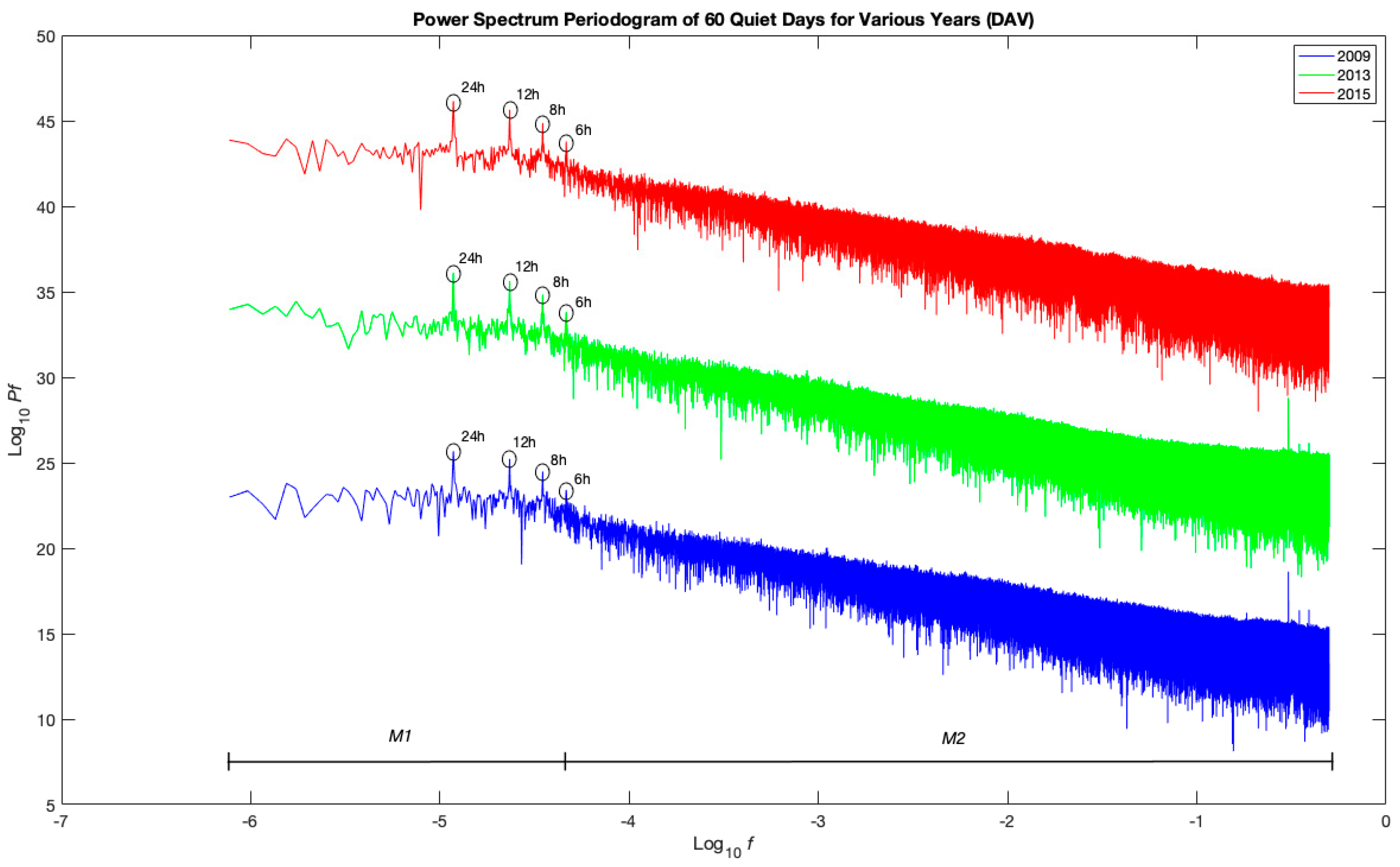
3.1. Fractal Properties of Quiet Day Geomagnetic Data

Figure 2 shows the power spectrum periodogram of 60 quiet days for the year 2009, 2013, and 2015. The blue spectra represents the year 2009, the green spectra represents the year 2013, and the red spectra represents the year 2015.

Table 2. Comparison of spectral peaks found in this study with Rabiu et al. [23] study.

This Study (DAV)		Rabiu et al. [23] (KOU and BNG)
Year	Existing Peaks (h)	Year	Existing Peaks (h)
2009	6, 8, 12, 24	1996	8, 12, 24
2013	6, 8, 12, 24	2000	6 *, 8, 12, 24
2015	6, 8, 12, 24	2002	8, 12, 24

* Only KOU station data showcases a peak at 6 h mark during that period.

shows the comparison of the spectral peaks found in this study compared with Rabiu et al. [23] study. The H-component data from Bangui station, Central African Republic (4.33° N, 18.57° E) and Kourou station, French Guiana (5.21° N, 307.27° E), which are abbreviated as BNG and KOU respectively, were chosen from Rabiu et al.’s study for comparison as these stations are located near the geomagnetic equator, to match the geomagnetic conditions of DAV station.

One common attribute that can be observed from the periodograms is the scaling properties. The change in data scaling rule indicates that the data has fractal properties [8] which were present in all of the periodograms analyzed in this study. The markings at the bottom of Figure 1—namely M1 and M2—indicate that all of the three periodograms have virtually the same scaling properties, with two distinct areas having different scaling rule.

While the identification of the point at which the scaling properties change is purely a qualitative process [52,53] and the use of power spectrum analysis as a method is not optimized to indicate precisely the scaling properties of a data [54], the fact remains that all the periodograms showed a change in scaling rule, a multifractal scaling [55,56]. Hence, all of the long-term quiet day data analyzed in this study exhibited fractal properties.

Aside from the scaling properties of the data, another attribute that can be observed from the periodograms is the spectral peaks. From Table 2, this study found that the year 2009, 2013, and 2015 showed the same number of peaks at the same hour marks; 6 h, 8 h, 12 h, and 24 h. As for the study of Rabiu et al. [23], all the years studied—1996, 2000, and 2002—also showed the same number of peaks at the same hour marks (albeit different from our findings of peaks) of 8 h, 12 h, and 24 h, with an exception for the peak at the 6 h mark which was only present in the KOU station H-component data for the year 2000. The existence of peaks itself is often attributed to several factors such as solar daily variation [14,23,57], lunar daily variation [58], and atmospheric tides [57,59]. Solar daily variation is caused by the rotation of the Earth, causing the Earth’s changes from night to day, which primarily causes the existence of the spectral peak at the 24 h mark. Lunar daily variation is caused by the motion of the moon revolving around the Earth, which causes the spectral peaks at the 12 h mark. The other factor that drives the existence of other peaks is the atmospheric tides caused by the rotation of the Earth, creating a global scale of oscillations which naturally have harmonic periods [59]. These harmonic periods correspond directly to the period in which the spectral peaks exist, which in turn, causes the remaining spectral peaks of 6 h and 8 h to exist.

It is concluded that all the long-term geomagnetic data over Southeast Asia during low, intermediate, and high solar activity showed fractal properties, and the existence of multiple spectral peaks showed that solar activity was not the sole driver of geomagnetic fluctuations. The findings in this study generally agreed with Rabiu et al. [23] study which used data from a different region. We came to this decision by considering the stations from which the data were used and the period of the study. The stations of DAV, KOU, and BNG are all located near the geomagnetic equator. As for the period of study, the years 2009, 2013, and 2015 correspond directly with the years 1996, 2000, and 2002. The years 2000 and 1996 were set during the solar maximum while the years 2002 and 2015 were set during the solar minimum. It is worth noting that this study did not subtract the baseline of H-component as implemented by Rabiu et al. [23]. In addition, their study analyzed the 1 h resolution data of H-component for the whole year while this study analyzed 1 s resolution data of H-component for selected quietest days of the year according to the international quiet day data. Nevertheless, the spectral peaks present in both H-component data are virtually the same.

3.2. Fractal Methods to Determine the Hurst Exponent of Geomagnetic Data

Table 3. Result of the accuracy test for each method using various synthetic fractional Brownian motion signals simulating the geomagnetic time series. The color gradient of orange-yellow-green-dark green indicates the degree of accuracy of each method, with orange being the least accurate while dark green being the most accurate.

Hurst (H)	PSA	RRA	DFA	r-DFA
0.1	0.04 ± 0.02	0.19 ± 0.02	0.09 ± 0.01	0.01 ± 0.03
0.3	0.20 ± 0.02	0.35 ± 0.02	0.31 ± 0.01	0.19 ± 0.03
0.5	0.40 ± 0.01	0.53 ± 0.02	0.51 ± 0.01	0.37 ± 0.03
0.7	0.44 ± 0.01	0.71 ± 0.03	0.70 ± 0.01	0.55 ± 0.04
0.9	0.41 ± 0.00	0.81 ± 0.07	0.91 ± 0.01	0.73 ± 0.04

shows the result of the accuracy test for each method using various synthetic fBm signals. The Hurst exponent values were obtained by using linear regression between parameters specified to be utilized in each method (Section 2.2), while the errors were based on the standard error of the regression which indicates how far the observed values are from the regression line. The color gradient of orange-yellow-green-dark green indicates the degree of accuracy of each method, with orange being the least accurate and dark green being the most accurate. The PSA method came out to be the least accurate out of all the methods, while the DFA came out to be the most accurate.

The PSA method is perfectly capable of identifying in detail the inflections and the scaling properties within a time series as demonstrated by the preceding part; a task that the other methods tested here were not that capable of. However, in measuring the overall Hurst exponent of a time series, it turns out that the PSA method was not that adequate at it. While it offered a great precise measurement by offering a small amount of standard error, the measurements just fell far off the mark. When subjected to fBm signals of H = 0.5 and above, it failed to produce a precise value for each noise and instead returned H ≃ 0.4—a point of saturation—for the noise H = 0.5, H = 0.7, and H = 0.9.

The RRA method may be the oldest method tested in this study, but according to our test, it is still adequate at measuring the overall Hurst exponent of a time series. The results produced by this method did not go that far off the mark, with a standard error level that left a lot to be desired—at worst, the amount of error was ±0.07—but was just acceptable given the age of this method. Moreover, the developments and improvements of various fractal methods over the period of half a century leaves us with plenty of methods to choose from, among them the DFA method.

Despite being the newest method in our test, r-DFA did not turn out to be the best method in this test. The r-DFA method was designed from the ground up, intended to be used for hydrogeological data. The incapability of the method in measuring the exact Hurst exponent of a synthetic geomagnetic time series does not come as a surprise since hydrogeologists undoubtedly have a different set of goals in using r-DFA as a method. In addition, there were several adjustments that had to be made in this test including the number of surrogate sets, the r-DFA order number, and the number of crossovers predetermined.

The number of surrogate sets utilized in this test was 5 sets instead of the supposed 100 sets the originators of the method had performed earlier. As for the r-DFA method, the results of the sixth order were compared with the other methods as the results yielded the nearest reading of the simulated signals. Additionally, there were no crossovers predetermined to exist in our testing. All these adjustments were made for the sake of comparison with the other methods and to reduce biases as the other methods had fewer variables to consider. Still, this study does not discredit the fact that it is an established method in the field of hydrology; however, it is just not adequate for our use in this study. The DFA method, over the years, has been stated as one of the most accurate fractal methods [10,12,14], and apparently it still is. It was found that the DFA method offered the most accurate measurement of Hurst exponent of time series compared to the other methods in this test. Not only that, but it also boasts the least amount of standard error compared to the others, at ±0.01 across all measurements. Therefore, going forward, we utilized the DFA method to characterize the various cases of quiet and disturbed days, in the form of short-term datasets, as well as long-term.

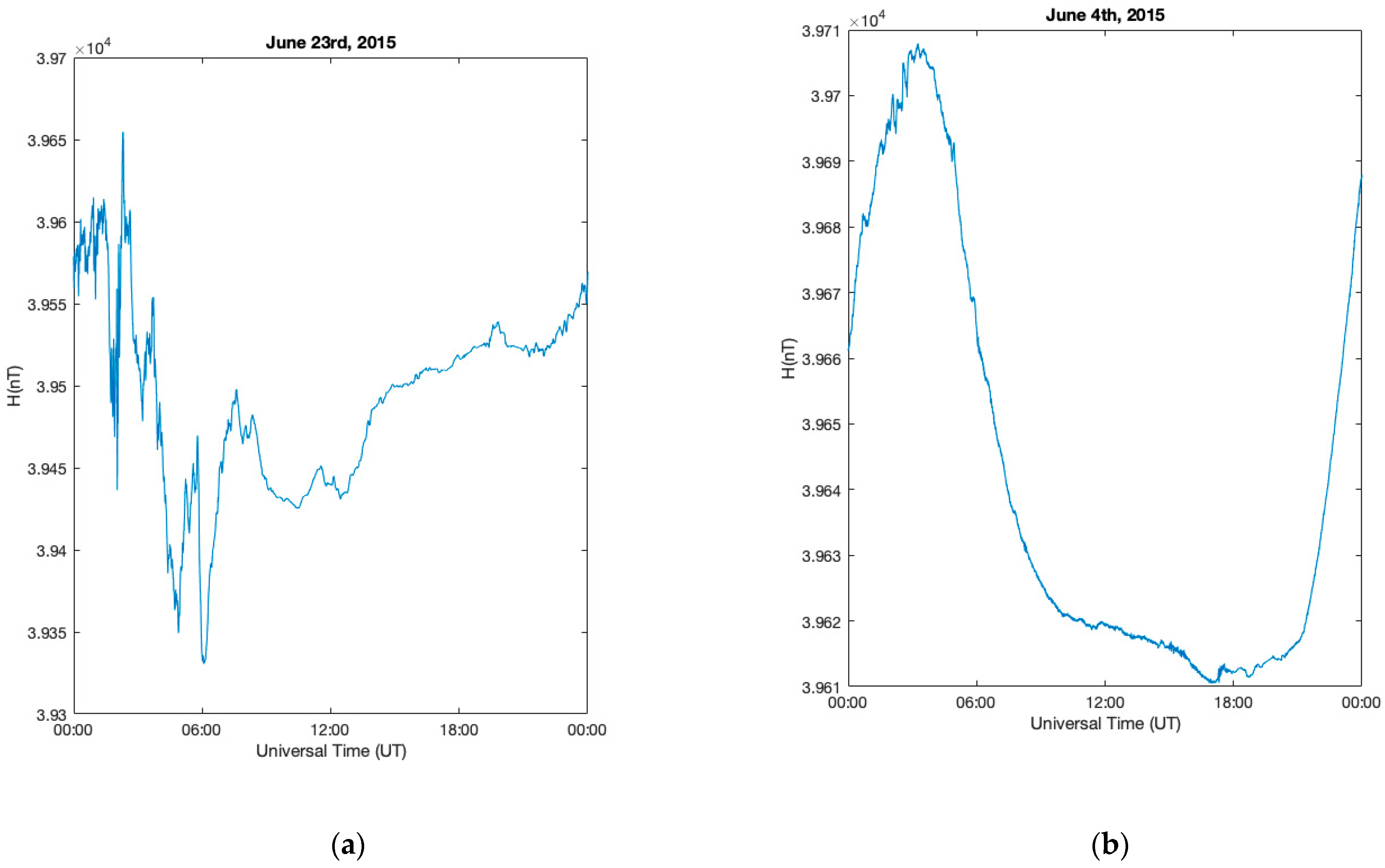
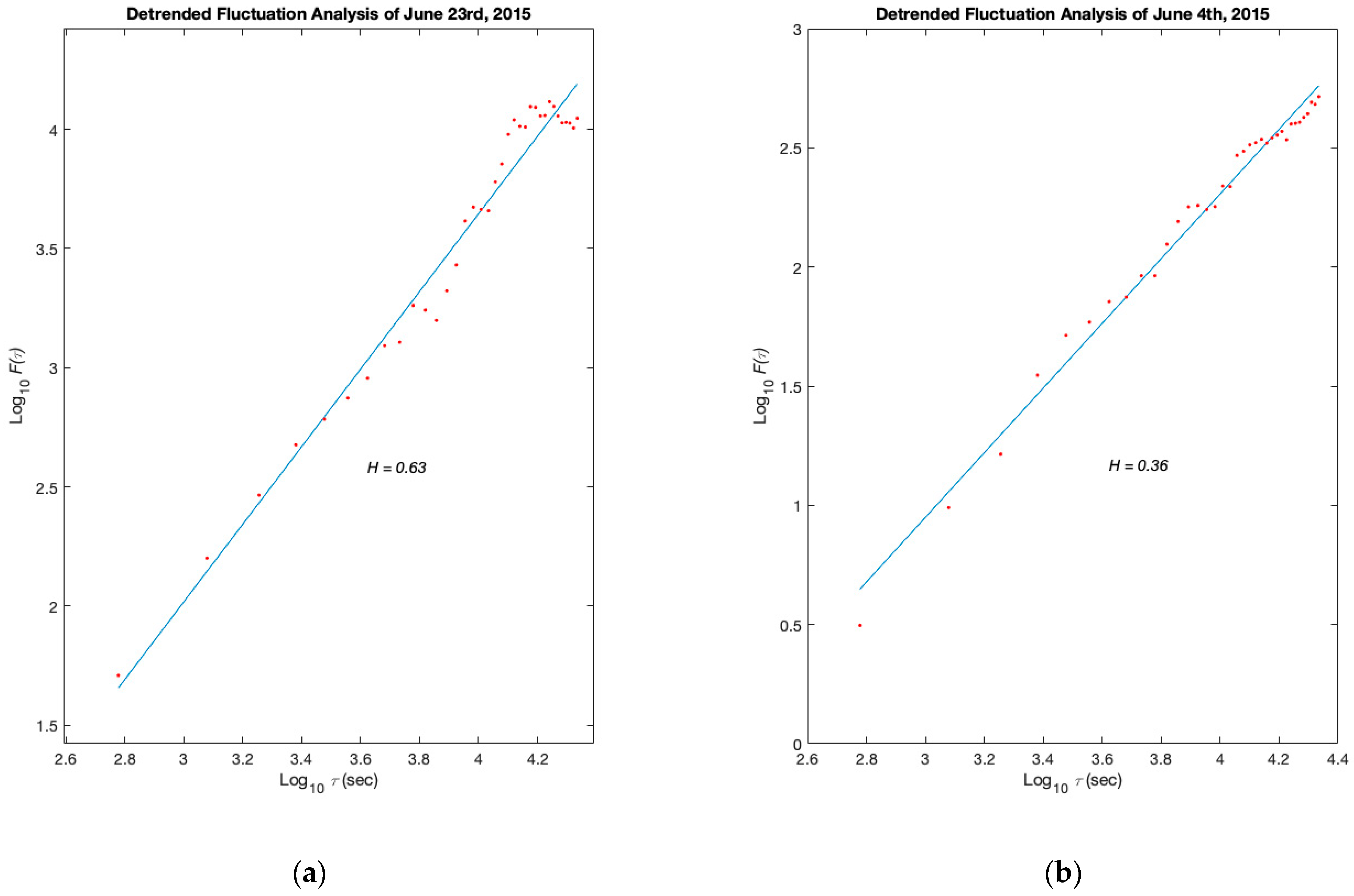
3.3. Characterization of Geomagnetic Data during Various Cases of Quiet and Disturbed Days

Figure 3 illustrates a sample of the DFA visualizations for several quiet and disturbed days analyzed in this section.

Table 4. The results of the short-term data analyses utilizing the DFA method. All results are in the parameter of Hurst exponent (H). Orange highlights indicate persistence tendencies, while green highlight indicates anti-persistence tendencies.

	Disturbed Day (All Major Events in One Year; Days with Dst < −200 nT)		Disturbed Day		Quiet Day
Station	2013	2015	17/03/2013	23/06/2015	26/03/2013	04/06/2015
DAV	0.56 ± 0.03 (3d)	0.58 ± 0.01 (7d)	0.62 ± 0.03	0.63 ± 0.05	0.36 ± 0.03	0.36 ± 0.03
LKW	0.69 ± 0.04 (3d)	0.74 ± 0.02 (5d)	0.68 ± 0.03	0.69 ± 0.05	0.38 ± 0.03	0.41 ± 0.04

shows all the Hurst exponent measurement results of various short-term data of disturbed and quiet days. There are three classifications of events of which results we would compare against one another, namely Disturbed Day (all major events in one particular year), Disturbed Day, and Quiet Day. All H-component data were sourced from DAV and LKW stations and analyzed using DFA imposed with spectral limit of 2.7788< log τ < 4.334 (τ = 6 h until τ = 10 min) following the approach made by previous studies [14,24].

The first class, the ‘Disturbed Day (all major events in one year)’, is the analysis of days with major geomagnetic events, namely days with Dst < −200 nT- in the year 2013 and 2015, utilizing the H-component data from DAV and LKW stations. All of the disturbed days’ data were concatenated into one single dataset according to its year and station, subject to each station’s availability of data, causing the variety of the datasets’ length to be analyzed using DFA. All of the measurements of the Hurst exponent for all datasets in this class showed persistence tendencies, with data from LKW in particular yielding far higher levels of Hurst exponent compared to DAV station.

The second class, the ‘Disturbed Day’, is the analysis of two days in which the lowest point happened to be during a particular major geomagnetic event in the year 2013 and 2015. The geomagnetic events chosen were the moderate geomagnetic storm of 17 March 2013 which happened during the March equinox, and the intense geomagnetic storm of 23 June 2015 which happened during the June solstice. All of the measurements of the Hurst exponent for all datasets in this class showed persistence tendencies, with data from LKW in particular yielding slightly higher levels of Hurst exponent compared to DAV station.

The third class, the ‘Quiet Day’, is the analysis of two quiet days which happened to be in the same period as the preceding analyses of the March equinox of 2013 and the June solstice of 2015. The days chosen were 26 March 2013 and 4 June 2015, both of which were the quietest day of each respective month. All of the measurements of the Hurst exponent for all datasets in this class showed anti-persistence tendencies, with data from LKW in particular yielding slightly higher levels of Hurst exponent compared to DAV station.

Overall, the results clearly established that disturbed days showed persistence tendencies while quiet days showed anti-persistence tendencies. This finding reaffirms the long standing theory that disturbed days generally has a higher level of scaling exponent compared to quiet days [12,14,60,61], resulting in a higher level of Hurst exponent. The higher level of Hurst exponent also indicates that the entropy of geomagnetic data strongly decreases during disturbed period [62,63]. It was also found that the results from LKW station were slightly higher than that of DAV station, with different levels of deviation for each class. The results of LKW station tend to deviate further from the results of DAV station in multiple day analyses compared to single day analyses, of which deviations still exist but negligible compared to the former. This deviation may be caused by the difference in the geographic state of each station [64,65], in that DAV and LKW stations are located in different parts of the Southeast Asia region, with LKW station located in the west while DAV station is located in the east. Further study utilizing geomagnetic and local wind data from different longitude sector, such as South America and India, is needed to draw a conclusion to confirm this hypothesis.

Table 5. Results of the long-term data analyses utilizing the DFA method. Orange highlights indicate persistence tendencies.

Period	Quiet Period	Disturbed Period
Year/Case	2009 (60d)	2013 (59d)	2013 (42d) (A-Index > 25)	2015 (60d)	2015 (58d) (A-Index > 25)
H	0.51 ± 0.03	0.55 ± 0.02	0.55 ± 0.02	0.55 ± 0.01	0.55 ± 0.01

shows all the Hurst exponent measurement results of various long-term data of quiet and disturbed period. For this part of the long-term data analysis, only DAV station data were utilized as this study only focused on comparing two conditions: the long-term quiet day data during low solar activity, the quiet period; and the long-term disturbed day data during intermediate and high solar activity, the disturbed period.

The DFA result of 60 quiet days in the year 2009 yielded the Hurst exponent measurement of 0.51 ± 0.03, showing persistence tendencies that bordered on random tendencies (H = 0.50). This finding is in line with the findings of Wanliss [12] and a couple of studies preceding it [66,67] in which these authors argued that the value of the Hurst exponent for the quiet time shall be around H ≃ 0.50. It is surmised that the random tendencies of the H-component data are caused by the nature of the geomagnetic data itself which is completely random and barely changes unless there is an external influence that acts upon it. The year 2009 itself was a year of low solar activity, suggesting that external influences were scarce and inconsequential compared to that of high solar activity. Therefore, geomagnetic activities during this time were generally random.

The DFA of 59 disturbed days in the year 2013 and 42 disturbed days that had A-index level above 25 in the year 2013 yielded the same level of Hurst exponent at 0.55 ± 0.02. For the DFA of 60 disturbed days in the year 2015 and 58 disturbed days that had A-index level above 25 in the year 2015, both analyses also yielded the same level of Hurst exponent at 0.55 ± 0.01. While both years showed persistence tendencies, the periods of solar activity in which both years were situated—intermediate solar activity for the year 2013 and high solar activity for the year 2015—caused little to no difference in the Hurst exponent. These findings reaffirm that disturbed days generally has a higher level of Hurst exponent compared to that of quiet days.

One last thing worth noting in our observations is that the value of Hurst exponent for analyses with shorter length of H-component datasets tend to skew extremely to either having persistence or anti-persistence tendencies, while longer H-component datasets tend to have value nearing random tendencies. Hence, it is surmised that as the H-component dataset gets longer, it tends to have more random tendencies, as evidenced by our findings. This particular characteristic may have a potential to be utilized in geomagnetic storm monitoring, particularly in the Southeast Asia region, using fractal analysis of real-time geomagnetic data as fractal analysis on short-term real-time geomagnetic data may indicate whether geomagnetic storm is still ongoing or otherwise, or showing potential to subside in the near future by referring to the Hurst exponent of the geomagnetic data.

4. Conclusions

In this work, we have analyzed the long-term quiet day H-component data of the Southeast Asia geomagnetic equatorial region during low, intermediate, and high levels of solar activity. We found that multifractal scaling exists in all of the data analyzed, signifying that the data exhibit fractal properties. We also found the existence of spectral peaks that were present at 6, 8, 12, and 24 h, which were marked throughout all of the years analyzed. This shows that there are external factors that drive the fluctuations of geomagnetic activity that are not limited to solar activity. The Detrended Fluctuation Analysis (DFA) method was found to be the best method to characterize fractal behavior of geomagnetic data. It was found that disturbed days generally showed a higher level of Hurst exponent compared to quiet days. As for the long-term data, disturbed days generally showed a higher level of Hurst exponent compared to quiet days, which had a value near H ≃ 0.50. This particular characteristic indicates that the Hurst exponent may have a potential to be utilized with geomagnetic data in monitoring geomagnetic storms in the Southeast Asia region. Additionally, we suggest future studies to identify whether the value of Hurst exponent will vary during different events that perturb daily variations of geomagnetic data such as earthquakes (lithospheric events) and solar flares (space events).

References

1. Kallenrode, M.-B. Space Physics: An Introduction to Plasma and Particles in the Heliosphere and Magnetospheres; Springer: Berlin/Heidelberg, Germany, 2004. [Google Scholar]
2. Owens, M.J.; Forsyth, R.J. The heliospheric magnetic field. Living Rev. Sol. Phys. 2013, 10. [Google Scholar] [CrossRef]
3. Bolzan, M.J.A.; Sahai, Y.; Fagundes, P.R.; Rosa, R.R.; Ramos, F.M.; Abalde, J.R. Intermittency analysis of geomagnetic storm time-series observed in Brazil. J. Atmos. Sol.-Terr. Phys. 2005, 67, 1365–1372. [Google Scholar] [CrossRef]
4. Oliver, R.; Ballester, J.L. Is there memory in solar activity? Phys. Rev. E Stat. Phys. Plasmas Fluids Relat. Interdiscip. Top. 1998, 58, 5650–5654. [Google Scholar] [CrossRef]
5. Zaourar, N.; Hamoudi, M.; Holschneider, M.; Mandea, M. Fractal dynamics of geomagnetic storms. Arab. J. Geosci. 2013, 6, 1693–1702. [Google Scholar] [CrossRef]
6. Bolzan, M.J.A.; Rosa, R.R.; Sahai, Y. Multifractal analysis of low-latitude geomagnetic fluctuations. Ann. Geophys. 2009, 27, 569–576. [Google Scholar] [CrossRef] [Green Version]
7. Addison, P.S. Fractal and Chaos: An Illustrated Course; IOP Publishing: London, UK, 1997. [Google Scholar]
8. Falconer, K. Fractals: A Very Short Introduction, 1st ed.; Oxford University Press: Oxford, UK, 2013. [Google Scholar]
9. Turcotte, D.L. Fractals and Chaos in Geology and Geophysics; Cambridge University Press: Cambridge, MA, USA, 1997; ISBN 9780521561648. [Google Scholar]
10. Weron, R. Estimating long-range dependence: Finite sample properties and confidence intervals. Phys. A Stat. Mech. Its Appl. 2002, 312, 285–299. [Google Scholar] [CrossRef] [Green Version]
11. Höll, M.; Kiyono, K.; Kantz, H. Theoretical foundation of detrending methods for fluctuation analysis such as detrended fluctuation analysis and detrending moving average. Phys. Rev. E 2019, 99, 1–20. [Google Scholar] [CrossRef] [PubMed] [Green Version]
12. Wanliss, J. Fractal properties of SYM-H during quiet and active times. J. Geophys. Res. Space Phys. 2005, 110. [Google Scholar] [CrossRef]
13. Wanliss, J.A.; Dobias, P. Space storm as a phase transition. J. Atmos. Sol.-Terr. Phys. 2007, 69, 675–684. [Google Scholar] [CrossRef]
14. Hamid, N.S.A.; Gopir, G.; Ismail, M.; Misran, N.; Hasbi, A.M.; Usang, M.D.; Yumoto, K. The Hurst exponents of the geomagnetic horizontal component during quiet and active periods. In Proceedings of the 2009 International Conference on Space Science and Communication, Negeri Sembilan, Malaysia, 26–27 October 2009; pp. 186–190. [Google Scholar]
15. Kantelhardt, J.W.; Koscielny-Bunde, E.; Rego, H.H.A.; Havlin, S.; Bunde, A. Detecting long-range correlations with detrended fluctuation analysis. Phys. A Stat. Mech. Its Appl. 2001, 295, 441–454. [Google Scholar] [CrossRef] [Green Version]
16. Dawley, S.; Zhang, Y.; Liu, X.; Jiang, P.; Yuan, L.; Sun, H. Statistical and Probability Quantification of Hydrologic Dynamics in the Lake Tuscaloosa Watershed, Alabama, USA. J. Geosci. Environ. Prot. 2018, 6, 91–100. [Google Scholar] [CrossRef] [Green Version]
17. Dawley, S.; Zhang, Y.; Liu, X.; Jiang, P.; Tick, G.; Sun, H.; Zheng, C.; Chen, L. Statistical Analysis of Extreme Events in Precipitation, Stream Discharge, and Groundwater Head Fluctuation: Distribution, Memory, and Correlation. Water 2019, 11, 707. [Google Scholar] [CrossRef] [Green Version]
18. Hekmatzadeh, A.A.; Torabi Haghighi, A.; Hosseini Guyomi, K.; Amiri, S.M.; Kløve, B. The effects of extremes and temporal scale on multifractal properties of river flow time series. River Res. Appl. 2020, 36, 171–182. [Google Scholar] [CrossRef]
19. Zheng, X.; Lian, Y.; Wang, Q. The long-range correlation and evolution law of centennial-scale temperatures in Northeast China. PLoS ONE 2018, 13, e0198238. [Google Scholar] [CrossRef] [PubMed]
20. Molkkari, M.; Angelotti, G.; Emig, T.; Räsänen, E. Dynamical Heart Beat Correlations as a Measure of Exercise Intensity. Sci. Rep. 2019, 2019, 13627. [Google Scholar]
21. Vipindas, V.; Gopinath, S.; Girish, T.E. A study on the variations in long-range dependence of solar energetic particles during different solar cycles. Proc. Int. Astron. Union 2018, 13, 47–48. [Google Scholar] [CrossRef]
22. Rifqi, F.N.; Hamid, N.S.A.; Yoshikawa, A. Possibility of robust detrended fluctuation analysis as a method for identifying fractal properties of geomagnetic time series. J. Phys. Conf. Ser. 2021, 1768, 012004. [Google Scholar] [CrossRef]
23. Rabiu, A.B.; Abdulrahim, R.B.; Garuba, O.A.; Adekanbi, O.O.; Alabi, S.A.; Ojurongbe, L.L.; Lawani, A.S. Occurence of Similar Periods in Geomagnetic Field Variations and Solar Activity. Arid Zone J. Eng. Technol. Environ. 2018, 15, 223–241. [Google Scholar]
24. Nasuddin, K.A.; Abdullah, M.; Abdul Hamid, N.S. Characterization of the South Atlantic Anomaly. Nonlinear Process. Geophys. 2019, 26, 25–35. [Google Scholar] [CrossRef] [Green Version]
25. Yumoto, K. Space weather activities at SERC for IHY: MAGDAS. Bull. Astron. Soc. India 2007, 35, 511–522. [Google Scholar]
26. Telesca, L.; Colangelo, G.; Lapenna, V.; Macchiato, M. Monofractal and multifractal characterization of geoelectrical signals measured in southern Italy. Chaos Solitons Fractals 2003, 18, 385–399. [Google Scholar] [CrossRef]
27. Malamud, B.D.; Turcotte, D.L. Self-affine time series: Measures of weak and strong persistence. J. Stat. Plan. Inference 1999, 80, 173–196. [Google Scholar] [CrossRef]
28. Mandelbrot, B.B.; Wallis, J.R. Some long-run properties of geophysical records. Water Resour. Res. 1969, 5, 321–340. [Google Scholar] [CrossRef] [Green Version]
29. Hurst, H.E. Long term storage capacity of reservoirs. Trans. Am. Soc. Civ. Eng. 1951, 116, 770. [Google Scholar] [CrossRef]
30. Ibe, L.; Ogunniyi Salau, T.A. Comparative Analysis of Rescaled Range Results of Normal and Abnormal Heart Sound Recordings. J. Eng. Res. Rep. 2019, 1–7. [Google Scholar] [CrossRef]
31. Yang, S.; Hu, X.; Liu, W.V.; Cai, J.; Zhou, X. Spontaneous combustion influenced by surface methane drainage and its prediction by rescaled range analysis. Int. J. Min. Sci. Technol. 2018, 28, 215–221. [Google Scholar] [CrossRef]
32. Xiao, Z.; Ding, W.; Liu, J.; Tian, M.; Yin, S.; Zhou, X.; Gu, Y. A fracture identification method for low-permeability sandstone based on R/S analysis and the finite difference method: A case study from the Chang 6 reservoir in Huaqing oilfield, Ordos Basin. J. Pet. Sci. Eng. 2019, 174, 1169–1178. [Google Scholar] [CrossRef]
33. Gkarlaouni, C.; Lasocki, S.; Papadimitriou, E.; George, T. Hurst analysis of seismicity in Corinth rift and Mygdonia graben (Greece). Chaos Solitons Fractals 2017, 96, 30–42. [Google Scholar] [CrossRef]
34. Yao, L.; Ma, R.; Wang, H. Baidu index-based forecast of daily tourist arrivals through rescaled range analysis, support vector regression, and autoregressive integrated moving average. Alexandria Eng. J. 2021, 60, 365–372. [Google Scholar] [CrossRef]
35. Akhmetova, A.Z.; La, L.L.; Murzin, F.A. Rescaled range analysis for the social networks. In Proceedings of the 5th International Conference on Engineering and MIS; ACM: New York, NY, USA, 2019; pp. 1–4. [Google Scholar]
36. Singh, A.K.; Bhargawa, A. An early prediction of 25th solar cycle using Hurst exponent. Astrophys. Space Sci. 2017, 362, 2–7. [Google Scholar] [CrossRef]
37. Klevtsov, S. Application of the Hurst index to evaluate the testing of information gathering system components. ITM Web Conf. 2019, 30, 04002. [Google Scholar] [CrossRef]
38. Peng, C.K.; Havlin, S.; Stanley, H.E.; Goldberger, A.L. Quantification of scaling exponents and crossover phenomena in nonstationary heartbeat time series. Chaos 1995, 5, 82–87. [Google Scholar] [CrossRef] [PubMed]
39. Pavlov, A.N.; Abdurashitov, A.S.; Koronovskii, A.A.; Pavlova, O.N.; Semyachkina-Glushkovskaya, O.V.; Kurths, J. Detrended fluctuation analysis of cerebrovascular responses to abrupt changes in peripheral arterial pressure in rats. Commun. Nonlinear Sci. Numer. Simul. 2020, 85, 105232. [Google Scholar] [CrossRef]
40. Pavlov, A.N.; Runnova, A.E.; Maksimenko, V.A.; Pavlova, O.N.; Grishina, D.S.; Hramov, A.E. Detrended fluctuation analysis of EEG patterns associated with real and imaginary arm movements. Phys. A Stat. Mech. Its Appl. 2018, 509, 777–782. [Google Scholar] [CrossRef]
41. Kuznetsov, N.A.; Rhea, C.K. Power considerations for the application of detrended fluctuation analysis in gait variability studies. PLoS ONE 2017, 12, e0174144. [Google Scholar] [CrossRef]
42. Tatli, H.; Dalfes, H.N. Long-Time Memory in Drought via Detrended Fluctuation Analysis. Water Resour. Manag. 2020, 34, 1199–1212. [Google Scholar] [CrossRef]
43. Liu, W.; Chen, W.; Zhang, Z. A Novel Fault Diagnosis Approach for Rolling Bearing Based on High-Order Synchrosqueezing Transform and Detrended Fluctuation Analysis. IEEE Access 2020, 8, 12533–12541. [Google Scholar] [CrossRef]
44. Blesić, S.M.; du Preez, D.J.; Stratimirović, D.I.; Ajtić, J.V.; Ramotsehoa, M.C.; Allen, M.W.; Wright, C.Y. Characterization of personal solar ultraviolet radiation exposure using detrended fluctuation analysis. Environ. Res. 2020, 182, 108976. [Google Scholar] [CrossRef] [PubMed]
45. Mallick, J.; Talukdar, S.; Alsubih, M.; Salam, R.; Ahmed, M.; Ben Kahla, N.; Shamimuzzaman, M. Analysing the trend of rainfall in Asir region of Saudi Arabia using the family of Mann-Kendall tests, innovative trend analysis, and detrended fluctuation analysis. Theor. Appl. Climatol. 2021, 143, 823–841. [Google Scholar] [CrossRef]
46. Skordas, E.S.; Christopoulos, S.-R.G.; Sarlis, N.V. Detrended fluctuation analysis of seismicity and order parameter fluctuations before the M7.1 Ridgecrest earthquake. Nat. Hazards 2020, 100, 697–711. [Google Scholar] [CrossRef]
47. Habib, A.; Sorensen, J.P.R.; Bloomfield, J.P.; Muchan, K.; Newell, A.J.; Butler, A.P. Temporal scaling phenomena in groundwater-floodplain systems using robust detrended fluctuation analysis. J. Hydrol. 2017, 549, 715–730. [Google Scholar] [CrossRef]
48. Li, Z.; Zhang, Y.-K. Quantifying fractal dynamics of groundwater systems with detrended fluctuation analysis. J. Hydrol. 2007, 336, 139–146. [Google Scholar] [CrossRef]
49. Little, M.A.; Bloomfield, J.P. Robust evidence for random fractal scaling of groundwater levels in unconfined aquifers. J. Hydrol. 2010, 393, 362–369. [Google Scholar] [CrossRef] [Green Version]
50. Mandelbrot, B.B.; Van Ness, J.W. Fractional Brownian Motions, Fractional Noises and Applications. SIAM Rev. 1968, 10, 422–437. [Google Scholar] [CrossRef]
51. Baillie, R.T. Long memory processes and fractional integration in econometrics. J. Econom. 1996, 73, 5–59. [Google Scholar] [CrossRef]
52. Zainuri, N.A.; Jemain, A.A.; Muda, N. Existence of fractal behaviour in ozone time series. J. Qual. Meas. Anal. 2016, 12, 97–106. [Google Scholar]
53. Shang, P.; Wan, M.; Kama, S. Fractal nature of highway traffic data. Comput. Math. Appl. 2007, 54, 107–116. [Google Scholar] [CrossRef] [Green Version]
54. De La Torre, F.C.; González-Trejo, J.I.; Real-Ramírez, C.A.; Hoyos-Reyes, L.F. Fractal dimension algorithms and their application to time series associated with natural phenomena. J. Phys. Conf. Ser. 2013, 475. [Google Scholar] [CrossRef]
55. Harte, D. Multifractals; Chapman & Hall: London, UK, 2001; ISBN 978-1-58488-154-4. [Google Scholar]
56. Lopes, R.; Betrouni, N. Fractal and multifractal analysis: A review. Med. Image Anal. 2009, 13, 634–649. [Google Scholar] [CrossRef]
57. Onwumechili, C.A.; Ezema, P.O. On the course of the geomagnetic daily variation in low latitudes. J. Atmos. Terr. Phys. 1977, 39, 1079–1086. [Google Scholar] [CrossRef]
58. Gouin, P. Reversal of the Magnetic Daily Variation at Addis Ababa. Nature 1962, 193, 1145–1146. [Google Scholar] [CrossRef]
59. Chapman, S.; Lindzen, R.S. Atmospheric Tides; Springer: Dordrecht, The Netherlands, 1969; ISBN 978-94-010-3401-2. [Google Scholar]
60. Balasis, G.; Daglis, I.A.; Anastasiadis, A.; Eftaxias, K. Detection of Dynamical Complexity Changes in Dst Time Series Using Entropy Concepts and Rescaled Range Analysis. In The Dynamic Magnetosphere; Liu, W., Fujimoto, M., Eds.; Springer: Dordrecht, The Netherlands, 2011; pp. 211–220. ISBN 978-94-007-0500-5. [Google Scholar]
61. Dias, V.H.A.; Franco, J.O.O.; Papa, A.R.R. Changes in fractal properties of geomagnetic indexes as possible magnetic storms precursors. arXiv 2006, arXiv:physics/0605170. [Google Scholar]
62. Donner, R.V.; Balasis, G.; Stolbova, V.; Georgiou, M.; Wiedermann, M.; Kurths, J. Recurrence-Based Quantification of Dynamical Complexity in the Earth’s Magnetosphere at Geospace Storm Timescales. J. Geophys. Res. Space Phys. 2019, 124, 90–108. [Google Scholar] [CrossRef]
63. Mourenas, D.; Artemyev, A.V.; Zhang, X.-J. Dynamical Properties of Peak and Time-Integrated Geomagnetic Events Inferred From Sample Entropy. J. Geophys. Res. Space Phys. 2020, 125. [Google Scholar] [CrossRef]
64. Hamid, N.S.A.; Liu, H.; Uozumi, T.; Yumoto, K.; Veenadhari, B.; Yoshikawa, A.; Sanchez, J.A. Relationship between the equatorial electrojet and global Sq currents at the dip equator region. Earth Planets Space 2014, 66, 146. [Google Scholar] [CrossRef] [Green Version]
65. Hamid, N.S.A.; Rosli, N.I.M.; Ismail, W.N.I.; Yoshikawa, A. Effects of solar activity on ionospheric current system in the Southeast Asia region. Indian J. Phys. 2021, 95, 543–550. [Google Scholar] [CrossRef]
66. Consolini, G.; Lui, A.T.Y. Symmetry breaking and nonlinear wave-wave interaction in current disruption: Possible evidence for a phase transition. Geophys. Monogr. Ser. 2000, 118, 395–401. [Google Scholar] [CrossRef]
67. Burlaga, L.F.; Klein, L.W. Fractal structure of the interplanetary magnetic field. J. Geophys. Res. 1986, 91, 347. [Google Scholar] [CrossRef]
Figure 1. An example of the H-component data. These in particular are single day data of 23 June 2015 (a) and 4 June 2015 (b) taken from DAV station. These data represent disturbed and quiet days, respectively, which are part of the short-term events analyzed in this study.
Universe 07 00248 g001
Figure 2. Power spectrum periodogram of 60 quiet days during low (2009), intermediate (2013), and high solar activity levels (2015). The circles on the spectra indicate the spectral peaks present in each year. The “M1” and “M2” markings at the bottom indicate areas with different scaling properties.
Universe 07 00248 g002
Figure 3. An example of the DFA visualization. These in particular are single day data of 23 June 2015 (disturbed day) (a) and 4 June 2015 (quiet day) (b) taken from DAV station.
Universe 07 00248 g003