Article

An Agent-Based Modeling Framework for Simulating Human Exposure to Environmental Stresses in Urban Areas

1
Graduate School Human Development in Landscapes, Christian-Albrecht-Universität zu Kiel, 24118 Kiel, Germany
2
Department of Mathematics, Center for Earth System Research and Sustainability (CEN), University of Hamburg, 20146 Hamburg, Germany
3
Institute of Geography, Center for Earth System Research and Sustainability (CEN), University of Hamburg, 20146 Hamburg, Germany
4
Meteorological Institute, Center for Earth System Research and Sustainability (CEN), University of Hamburg, 20146 Hamburg, Germany
*
Author to whom correspondence should be addressed.
Submission received: 26 February 2018 / Revised: 4 April 2018 / Accepted: 13 April 2018 / Published: 17 April 2018

Abstract

:
Several approaches have been used to assess potential human exposure to environmental stresses and achieve optimal results under various conditions, such as for example, for different scales, groups of people, or points in time. A thorough literature review in this paper identifies the research gap regarding modeling approaches for assessing human exposure to environment stressors, and it indicates that microsimulation tools are becoming increasingly important in human exposure assessments of urban environments, in which each person is simulated individually and continuously. The paper further describes an agent-based model (ABM) framework that can dynamically simulate human exposure levels, along with their daily activities, in urban areas that are characterized by environmental stresses such as air pollution and heat stress. Within the framework, decision-making processes can be included for each individual based on rule-based behavior in order to achieve goals under changing environmental conditions. The ideas described in this paper are implemented in a free and open source NetLogo platform. A basic modeling scenario of the ABM framework in Hamburg, Germany, demonstrates its utility in various urban environments and individual activity patterns, as well as its portability to other models, programs, and frameworks. The prototype model can potentially be extended to support environmental incidence management through exploring the daily routines of different groups of citizens, and comparing the effectiveness of different strategies. Further research is needed to fully develop an operational version of the model.

1. Introduction

1.1. Human Exposure to Environmental Stresses

Human health is closely related to the surrounding environment. People are exposed to a variety of factors that can be hazardous to health, including their physical living environment. A series of climate change-related risk factors (rising sea levels and storm surges, heat waves and droughts, typhoons and extreme precipitation, inland and coastal floods) pose serious risks to human society [1]. The strength and frequency of many risk factors tends to increase. The occurrence of these hazards often stresses human health and welfare, e.g., through diseases, property damage, economic loss, and ecological environment degradation. For instance, extreme rainfall causes urban flooding, which often leads to large economic losses and serious threats to urban safety [2], while heat waves are harmful to public health, especially to vulnerable groups, which is the most significant reason of weather-related deaths [3]. At the same time, the impacts of air pollution, drought, wind, snow, and freezing weather on the normal operation of the city are also becoming increasingly prominent [4].
Over the last decade, the combined effects of a set of environmental factors on health concerns have received growing attention in research, including a rising awareness of the risks posed by heat waves, air pollution, noise, visual and social loads, and similar phenomena [5,6,7]. Most studies have focused on one or two of these environmental stressors and found significant effects on health risk.

1.2. Human Health in Urban Environments

Cities are highly artificial environments that are quite special and different from the natural environment in which humans have always lived. Modern cities can improve health via the provision of services as well as material, cultural, and aesthetic attributes. They also offer opportunities for cost-effective interventions that can serve many people. Urbanization represents both opportunity and risk, and offers a fresh set of challenges for those concerned with protecting and promoting human health and well-being. On the other hand, urban environments can be highly stressful, where humans are exposed to multiple sources of environmental discomfort, such as air pollution, high temperature, noise, odor, and social burdens [8]. As a result, the health and well-being of humans can be negatively affected by the urban environment [9]. Humans in cities often cannot avoid being exposed to stressors, as they must work, shop, travel, or entertain in the cities. Working or staying for a long time outside is the main way that people are exposed to a stressful environment, followed by traveling, particularly walking and cycling [10]. Even when remaining indoors, people are exposed to risks of high temperature, noise, and air pollution, as their effects often can penetrate into buildings.
The overlap of global climate change and urbanization makes cities the places where risks are concentrated and intensified due to the high density of population, building, traffic, and other urban infrastructures [6,11]. Environmental hazards remain, and new threats have emerged [12]. Urban air pollution—a significant proportion of which is generated by vehicles, as well as industry and energy production—is estimated to kill some two million people annually [13]. Such stresses can worsen in the future, considering that more than half of the Earth’s population currently lives in cities (54% by 2014), and that this proportion will rise up to 66% by 2050 [14].
Over the next 30 years, most of the world’s population growth will occur in the cities and towns of developing countries, mainly in Africa and Asia [14]. As urban populations grow, the quality of the urban environment will play an increasingly important role in public health with respect to issues ranging from solid waste disposal, the provision of safe water, sanitation, and injury prevention, to the interface between urban poverty, environment, and health [15].

1.3. Dynamics of Environment Exposure

Since humans are an active component of cities, human exposure to the urban environment is strongly linked to various processes that are inherent in human mobility, distinctly local and individual characteristics (e.g., clothing type, traveling tool, physical quality) and finally, to the quality of the natural, built, and social environment [9,16]. While people move, the environment in which they are located and their exposure to the environment changes dynamically. In addition, available evidence indicates that personal exposure to multiple pollutants is not adequately characterized, because the time that people spend in different locations and their activities vary dramatically with age, gender, occupation, and socioeconomic status [17,18]. Thus, the exposure is dynamic, and the challenge for research is to analyze the complex relationships between the individuals and their local environment, explore new exposure mechanisms under mobility, and identify universal and specific local conditions in the urban context [19].
Preventing and reducing harmful exposure requires an understanding of exposure dynamics, in particular its sources, intensity, extension, duration, process, and impacts [20]. Different microenvironments (e.g., temperature, humidity, shadow, wind) and activities (e.g., working, shopping, and entertaining) lead to everyday exposure levels of people moving in the city. Yet, if the threats can be so different, they could affect the same people. The challenge is thus to find innovative, efficient approaches to collect, organize, store, and communicate exposure data on an individual level, while also accounting for the inherent spatial–temporal dynamics.
Models are appropriate tools to reach understanding on this issue. A dynamic individual exposure model that is able to evolve as the individual moves would lay the basis for an assessment of the exposure level by providing reliable and standardized information on the exposed objects across a vast range of human activities [21]. In this paper, we conducted a thorough literature review on different types of exposure models, their characters and advantages, and both their spatial and socioeconomic dimensions. By identifying research gaps in recent exposure models, we emphasize the capacity of an agent-based model to fill the gaps and present an agent-based model framework to integrate the dynamic and individual features of human exposure in urban environments. A prototype of the model framework is applied in the case of Hamburg. The aim of the paper is to assess the challenge of implementing a dynamic exposure model for individuals of different but specific mobility within an agent-based modeling framework.

2. Modeling Approaches for Assessing Environment Exposures

A wide variety of exposure models are employed for assessments of human exposure to environment stresses. These existing exposure models can be broadly categorized according to their target objects: modeling of exposure sources, exposed objects (receptors), and of accumulated exposure consequences (integrated in Table 1). In this section each of these basic types of exposure models are briefly described, along with inherent strengths or weaknesses, followed by an analysis of the gaps and capacities of an agent-based model.

2.1. Modeling of Exposure Sources

The modeling techniques that have been adopted for current exposure models have evolved along distinct pathways for the various types of exposure sources [22]. An elementary step towards a modeling assessment of the exposure to new compounds or pollutants (chemicals, materials) is to estimate their environmental concentrations [23]. Most of the studies focusing on the concentrations of environmental risk factors use mathematical models (mainly fluid dynamical models) that are based on measurements extracted from a small number of fixed climatic monitoring stations for indoor and outdoor urban types of environments [24]. Jerrett, et al. [25] reviewed these models and sub-classified them as (i) proximity models; (ii) interpolation models; (iii) land-use regression models; (iv) dispersion models; and (v) integrated meteorological emission models. Geographical information systems (GIS) are often applied in these models to demonstrate the spatial and temporal patterns of environmental pollutants. Nevertheless, these kinds of models aim to extrapolate the concentration distribution of the environmental stressors through considering various factors that affect patterns of distribution in the research area, which is often (part of) a city (Brauer et al. [26], and others in Table 1).
Schnell et al. [24] criticized such models: (1) they underestimate concentrations of risk factors using limited monitoring measurements; (2) the complexity of pollutant distribution patterns was hardly accurate in these models; and (3) the indoor environment was ignored when using only outdoor monitoring data. Beyond Schnell’s criticism, these models mostly focus on a single stressor of concern, and describe a few pathways through which the receptor—either a human or another organism—can be exposed [27]. However, awareness is growing that exposure to single stressors is the exception rather than the rule [28]. In practice, organisms are often exposed to multiple stressors, e.g., extreme weather, a chemical mixture, or a combination of chemical, biological, and physical agents. Exposure to multiple stressors may take place concurrently or sequentially, and the individual stressors may or may not interact [28].
To some extent, the effect of stressor concentrations cannot really be represented by exposure models if there is no specified subject that suffers from the stressors. Moreover, due to raising concerns of people-centered urban management, to date, the monitoring of urban environments has not taken into account the dynamism of urban daily life [19]. Humans in the city are actively mobile, which greatly influences the consequence of individual exposures. Therefore, current studies intend to combine the modeling of exposure sources with human and/or other exposed subjects [20,29].

2.2. Modeling of Population Exposure

Models of population exposure go a step further than stressor concentration models. These models generally assess the size of a population as well as the area and/or property that is exposed to certain stressor concentrations, and may also compare the exposure level of sub-regions or sub-groups (Table 1). Natural hazards such as flooding, sea level rise, snow avalanches, and droughts are among the most targeted exposure sources. For example, the nationwide exposure assessment in Austria covers river flooding, torrential flooding, and snow avalanches [35]. A mapping study of flood exposure detected flood inundation areas and the affected people [46], which indicated that exposure depends strongly on the temporal and spatial dynamics of the distributed population. A few studies also estimated the global exposure to floods and revealed the economic exposure, population exposure, and geographical distribution of regional exposures [34,47,48]. Overall, these modeling approaches help identify highly exposed regions, and are an important and suitable tool to inform regional or nationwide adaptation. Also, the impact of the structure and morphology of cities on the heat stress exposure of urban commuters has been investigated by combining a simple heat stress model with a traffic model that can track certain groups of commuters [40].
Population exposure models have been widely applied to explore human exposure to air pollutions. Hystad et al. [36] created national pollutant models to produce estimates of population exposure to five common air pollutants (PM2.5, NO2, benzene, ethylbenzene, and butadiene) in Canada. Global and regional exposure to black carbon [37], metals [49], and ozone [26] were also estimated using similar approaches. Besides, a noise exposure model for London indicated that over one million residents were exposed to high daytime and night-time noise levels [38]. Modeling of traffic pollution exposure in Toronto revealed that the areas and periods with the highest pollution were along roadways at peak levels of traffic, but the highest population exposure occurred in the central business district due to the higher population density [39].
Population exposure models often place strong emphasis on the geographical distribution of populations and stressors, as well as their estimated level or intensity of exposure, which might be called population-weighted stressor concentrations [37]. These models have advantages in identifying geographic areas, which are usually larger than a city, where hot-spot exposures are a potential risk to human health, and are informing decision making to reduce exposure inequalities [49]. New developments in sensor technology now enable us to monitor multiple stressors and personal exposures in activity spaces and fields of varying concentration [16].

2.3. Modeling of an Individual’s Exposure Degree

Individual exposure models simulate the exposure level of each receptor based on its individual characteristics and within a preset specific route and/or space (Table 1). These approaches are often seen in mobility-related exposure studies using empirical or experimental traffic data for specific individuals [43,50]. Leyk et al. [45] presented a spatial individual-based model prototype for assessing the potential pesticide exposure of farm workers that tracked their individual movements and activities. Similarly, more complex modeling tools were developed for the quantification of human exposure to traffic-related air pollution within distinct microenvironments by using a GPS trajectory analysis of the individuals in the city area [10,24]. The findings of these approaches showed that people were exposed to environmental sources of discomfort while performing their daily life activities [7,10]. These studies suggested a shift from measuring environmental conditions in fixed monitoring stations to monitoring with mobile portable sensors [44,51].
Individual exposure models were applied in both human models and wildlife models. Loos et al. [28] compared five human and five wildlife receptor-oriented exposure models, and identified similarities regarding their exposure receptor, chemical stressors, and the extent of model validation, as well as differences related to the simulation of behavior and the representation of individuals and space. In addition, an individual receptor can be considered as an integrator of different stressors to which it is exposed while moving through space and time. Therefore, exposure models for multiple stressors should primarily focus on the receptor, and not on the stressor(s). A few studies have indeed reported the applicability of individual-oriented models in modeling noise, black carbon, particle number concentrations, and multiple chemicals [41,44].
The assessment of individual exposure often aims to determine the total degree or intensity of exposure along a process of moving between different spatial sites. Sampling approaches are generally applied to collect exposure data at different times and locations, which are often along a planned routine path in a city. The assessment shows that the consequences of accumulated exposure levels are often a function of the stressor concentrations and the durations of being exposed: the so-called time-weighted stressor concentrations [52]. As indicated in Table 1, most individual exposure models do not consider human exposure as a dynamic process, but rather as a summary over several time points/periods. This may be discussable in instances of long-term continuing environment threats, such as for example, a heat wave that lasts several days. In practice, the monitoring of individual exposure is limited to studies with a small number of individuals because of the high costs and complex organization that is associated with such measurements [10,51]. The results tend to be accurate and reliable at the personal level, although they do not show a big picture of the exposure patterns for the whole city or area.

2.4. Research Gaps and Capacities of Agent-Based Modeling

As shown above, dozens of studies have measured the concentrations of numerous stress sources in the different media to which humans are exposed. Others have catalogued various exposure pathways, and identified the duration and accumulation of exposure for the general population. All of this information allows better estimates of exposure. However, literature reviews have demonstrated that the role of individual mobility for exposure was less explored and based on limited monitoring data of personal samples [19]. The relationship between individual heterogeneity and uniform group patterns, especially for peak exposure in “hot spots”, is still insufficiently addressed, and the contribution of mobility-related exposure is not clear [7]. In addition, the dynamic process of changing exposure to various individuals requires innovative models that can identify the emerging non-linear patterns of collective exposures. We hypothesize that a computer simulation tool with a large number of individual random activities in different types of environments can provide a better understanding of the consequences of human exposure to environmental risk factors throughout the concerned spatial and temporal range.
To fill the research gaps and test the hypothesis, we recommend the development of an overall framework to screen the exposure source concentrations, collect better source and receptor data, explore the spatial and temporal variability of individual exposure concentrations, and demonstrate exposure processes and emerging collective exposure patterns. While a few researchers have mentioned similar ideas, taking into account activity spaces and daily mobility in measuring environmental exposures [7,19,53], the present study is a practical effort to implement them. An agent-based model (ABM) is a suitable tool to implement such dynamic non-linear and collective simulations, as reviewed in existing studies on coupled human–nature systems [54].
An agent-based model considers the essential known and measurable aspects of an agent, and acknowledges the nonlinearities and underlying dynamic processes [54,55,56,57]. An agent-based approach can make an important contribution to improving health and well-being, both at individual and collective group levels. In an ABM, agents are described by self-contained or self-consistent algorithms (realized in computer programs) that interact with their environment and one another; these algorithms can also be designed and implemented to describe rule-based behaviors and the modes of interaction between observed social entities [55,58,59].
Regarding the field of environmental exposure studies, ABMs have the advantage of simulating the exposure consequences of individual activities and patterns of collective group exposures, and suggesting exposure reduction strategies accordingly. Currently, there is limited understanding of complex mobility exposure to environmental stresses in the specific urban context. There is a need to develop an innovative and operational approach to understanding urban health and well-being that integrates individual characters within a mobility context. This, in turn, will help to integrate substantive considerations of individual well-being into the long-term planning, development, and management of urban environments. Exposure estimates to atmospheric pollutants can address individuals (personal exposure) or large population groups (population exposure), and can be based on direct (exposure monitoring) or indirect methods (exposure modeling). Efforts aiming at providing useful global models have given rise to freely available, web-based databases; each acts as a collector of the different data and models representing geophysical and meteorological risks.

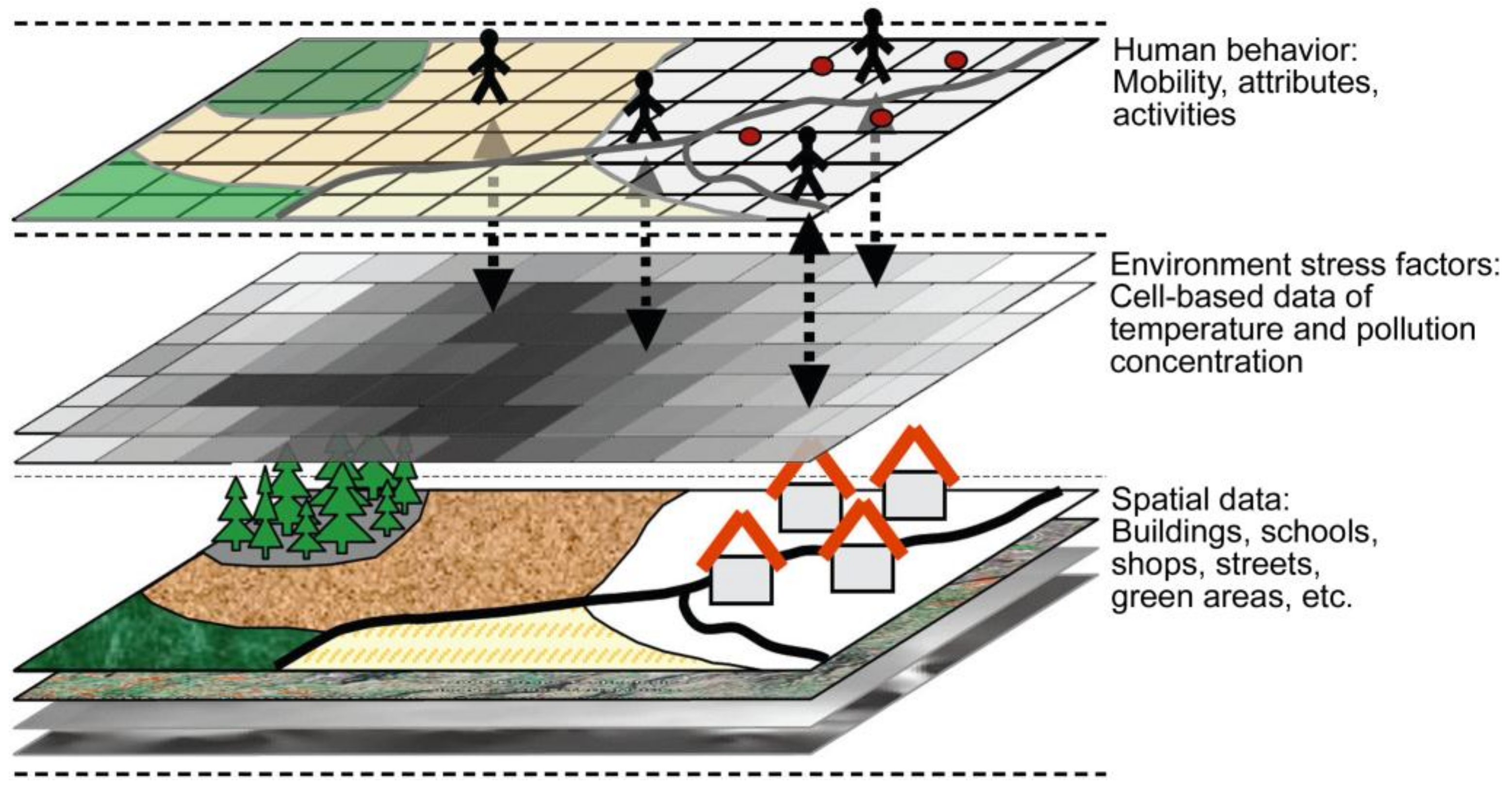
3. An Agent-Based Modeling Framework

In the present study, an agent-based modeling framework of urban environment stresses is developed to quantify human exposure within distinct microenvironments using a novel approach based on an analysis of the daily routines of individuals. Subsequent sections provide the context of the model environment and its implications for health, and outline a conceptual framework for the study of health and well-being in and between urban spaces. Finally, guidance on research criteria and the use of a systems approach is offered to prospective investigators for the development of a new research design.

3.1. Model Structure

The model framework is structured in three overlapping layers: spatial data of the concerned urban environment, concentrations of environmental stress sources, and human activities. Figure 1 illustrates the ABM used in this paper.
In this framework, a specific map will be used to represent the city with buildings, streets, shops, green areas, etc. (lower layer in Figure 1). Within this framework, spatial data of the changing concentration patterns of the environmental stress factors are the key pre-set inputs of the system (center layer in Figure 1). Agents with initial attributes act daily to work, rest, entertain, shop, take care of children, and follow certain paths to work (top layer in Figure 1). Once the prototype model is initialized, agents dynamically follow their daily life according to predetermined rules that are set according to empirical studies and specific surveys. Depending on their normal lifestyles (different among agents), as well as the environment stress factors of their location, they suffer from or reduce exposure levels. A simulation during a heat wave or air pollution event, with a typical time-step of minute, and a period from hours to days, would report a cumulative exposure level for each agent, and a collective pattern of all of the agents in the study area. The loops of agents’ daily activities and the evolution of the stressful factors drive the model to run step by step, so that the exposure process can be analyzed. Finally, the model produces summary information that can be used to diagnose both individual and collective exposure and inform relevant exposure reduction strategies. Further details of the model components are introduced in the following sections.

3.2. Modeling Environment

The modeling environment includes two parts: the natural environment of the studied city area, and the stressed environment of a heat wave or air pollution event. The natural environment of the city is represented by an integrated computable map of land-use data, street and building information, key sites, and so on. Such data are usually available in GIS format.
In addition to data from the urban environment, geospatial data for the stressed environment are needed to map the impact on agent movements. Environmental stressors such as high temperatures or air pollution can be taken from measurements or atmospheric model simulations. These are usually gridded datasets with a fixed spatial resolution. The temporal resolution typically varies between minutes and hours. For simulating the exposure to stressors, both high spatial and temporal resolutions are desired. However, there are limits that are set by the availability of observations, the resolution of the models, or the computing resources (e.g., disk space, working memory, or computing time). Increasingly, digital crowdsourcing data become available.
The introduced modeling framework aims to simulate the exposure to air pollution and heat stress in an urban area. Air pollution is elevated in urban areas, which is mainly due to emissions from traffic (fossil fuel-driven vehicles and ships), industry, and residential heating [16,20]. Therefore, high concentrations can be expected near big roads, as well as harbor and industry areas [21]. Pollutants range from larger particles such as particulate matter (PM) to gases such as ozone, NOx, CO, etc. Most of them are formed after several chemical reactions [27]. Hence, chemistry models are applied to simulate the concentration levels within urban areas [60]. The emissions of chemicals, which are crucial for the chemistry model, are usually estimated from traffic, census, and monitoring stations [27].
It is well known that due to the heterorganic surfaces and three-dimensional structures (e.g., buildings, trees, bridges, etc.) temperatures and heat stresses can vary strongly within a city [61]. At night-time, the so called urban heat island (UHI) can develop for low wind speed and cloud cover [62]. The UHI refers to higher near-surface temperatures in urban areas compared with the rural surroundings. Also, during the day, temperatures vary within the city. Especially, green and blue areas (e.g., parks, lakes, rivers, etc.) have a cooling effect during the day. Since humans do feel the environment as a combination of meteorological variables such as temperature, humidity, wind speed, and long and shortwave radiation, rather than temperature alone, so-called biometeorological indices are computed that summarize the combined effect of the thermal environment on the human heat budget of a person [63]. The developed prototype uses artificial temperature data that is randomly chosen from a typical temperature range for Hamburg to validate the model, because high-resolution daily or hourly temperature or heat stress data for Hamburg are only available for periods with a length of 3–4 days in summer [64,65].

3.3. Agent Attributes and Behaviors

The urban population is quite diverse, consisting of people of different ages, genders, living and working locations, social backgrounds, lifestyles etc. Hence, they all show unique behavior. Modeling each urban dweller of a city such as Hamburg with 1.7 million citizens is not feasible due to computing constraints, and more importantly due to the lack of available data. However, it is possible to group people with similar attributes and behaviors to agent types based on surveys, traffic data, and data from public transport companies. As summarized in Table 2, the behavior of urban dwellers can depend on their age, gender, work, income, education, living and working location, and access to cars or public transport, as well as the environmental conditions (e.g., rain, temperature, and pollution levels). Table 2 also gives examples for possible agent groups that can be implemented in an ABM. Crowdsourcing information on detailed time–location data can also be collected for each individual at each moment by GPS-equipped mobile phones, offering many advantages over traditional time–location analysis, such as high temporal resolution and minimum reporting burden for participants.

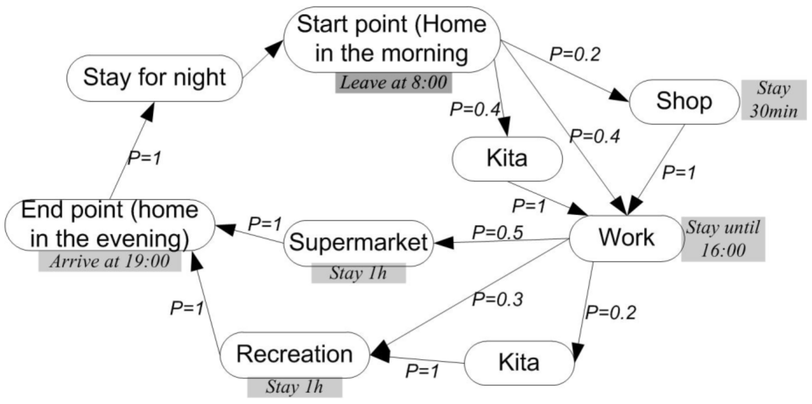
3.4. Daily Routines of Agents

As mentioned before, agents have goals that they are following. These could be to go to work every day, take children to school or day care, etc. To facilitate the modeling, it is hypothesized that the daily routine of a certain group of agents is uniform. This makes it possible to simulate as many agent types as determined in grouping processes. According to the grouping properties of the agents, the empirical data and survey data are used to generate synthetic daily routines, with agent priorities for each option of the population commuting between different directions. To capture variability in the travel survey and uncertainties in behavior, the synthetic daily routines can be described as action priorities p. An example of a synthetic daily routine for a female agent who is employed, aged 30–45, and has one child is shown in Figure 2. In this example, the agent starts the day at 8 am with a standard deviation of 15 min. They then travel via school to drop off their children, and then onto work with a 0.2 priority of visiting the shops for a while en route, and so on. Parts of this daily routine can be different among agents of the group, e.g., the time spent in a shop, but the agents in this group all have to visit many places on the route.

3.5. Model Formulation

In the model, agents are commuting to work using different means of transport (i.e., car, bike, and public transport), as well as different routes, where they are exposed to different air pollution and temperature levels. The decision on which means of transport to use is based on the priority p for the k different choices, while the change of the priorities is based on a value function v, which in our case is the weighted sum of commuting costs cc, commuting time ct, deviation from a desired temperature dt (|T-Tdesired|), and the accumulated exposure to NO2 eNO2 (Equation (1)). The indices min and max represent the respective minimum and maximum value elements. An exposure to NOx occurs if a harmful threshold of 30 µg/m3 is reached in the case of Hamburg (Federal Environment Agency [66]). For an ABM, it is necessary to introduce a value function that drives the decisions of agents where the most preferred option is reached for v i , k = 0 . This function is based on the work of Scheffran and BenDor (2009) [66], and was adapted for the exposure ABM:
v i , k = ( α i ( c c k c c m i n c c m a x c c m i n ) + β i ( c t k c t m i n c t m a x c t m i n ) ) + γ i ( ( d t k d t m a x d t m i n ) + ( e N O 2 k e N O 2 m i n e N O 2 m a x e N O 2 m i n ) ) 0
where i is the agent index and element in [1, N], and k is the action path and element in [1, K].
The parameters α, β, and γ represent the relevance (weight) of each term, which differ between the agents with respect to their characteristics. The sum of all three parameters is 1. In order to make the different terms comparable, they are normalized with respect to their maximum and minimum. Hence, values can range from 0 to 1. For simplicity, the normalized exposure to high/low temperatures and the exposure to NO2 are combined into one exposure term in the current version of the model. This means that they are currently equally weighted, because it is not yet clear how to combine the effect of exposure to both stressors on the health of the agents.
Following Scheffran and BenDor [67], the change in the priority of agent i for action path k in each time-step is proportionate to the actual priority and the difference between the agent’s value for path k and the weighted average value over all of the pathways, which are normalized by the sum of values:
Δ p i , k = a i × p i , k ( v i , k l = 1 n v i , l × p i , l | l = 1 n v i , l | )
where ai is the adaption parameter of agent i, representing how fast an agent adapts and reacts to value changes. The dynamics meets the side conditions 0 p i , k 1 , k = 1 n p i , k = 1, k = 1 n Δ p i , k = 0. Thus, agents allocate fractions of their resources to action paths k, which can switch between 0% and 100% for exclusive pathways. After each time-step, new priorities are computed (Equation (3)).
p i , k ( t ) = p i , k ( t 1 ) + Δ p i , k ( t 1 )
The values for the exposure are computed during the model run, while the values for costs and the commuting time are currently predefined.
The time-step that is used in the model depends on the temporal resolution of the input data, as well as on the desired changes in the actions of the agents. Based on those resolutions, the model simulation selects an appropriate ‘time-step’ to integrate the different data, which can range from minutes to days. Typical time-steps as used in the literature were 30 min [45], one hour [7], or one day [20] for exposure models. In instances of coarse data resolution, the time resolutions can be simply smoothed using linear time interpolation (which is the same as space interpolation). In our prototype model of the Hamburg case, the time-step of one day was used (Section 4).

3.6. Exposure Assessment

At each position x, which is visited/passed by an individual agent at time-step t, the value of the underlying stress factor H(x,t) is recorded. The potential external exposure Ei(x,t) of an individual i at location x for time-step t is then estimated using the equation:
E i ( x , t ) = A i ( x , t ) × H ( x , t )
where Ai(x,t)→[0,1] is the weight related to the activity performed by individual i at location x and time-step t under the considered safety level. Thus, the values of Ai(x,t) change over time, depending on the activity performed at time-step t and the safety level assumed for this individual i (attribute value from Table 2). The values Ei(x,t) could be expressed as concentrations if field measurements were available, since they are derived from H(x,t) values. In the case of an uniform pattern of the stressor concentration, the H(x,t) would be static, and the sum exposure of the agent would depend on its activity intensity and exposed time. In the case of Ai(x,t) = 1, H(x,t) being translated into Ei(x,t) without weighting, the exposure is solely determined by the environmental stressors.

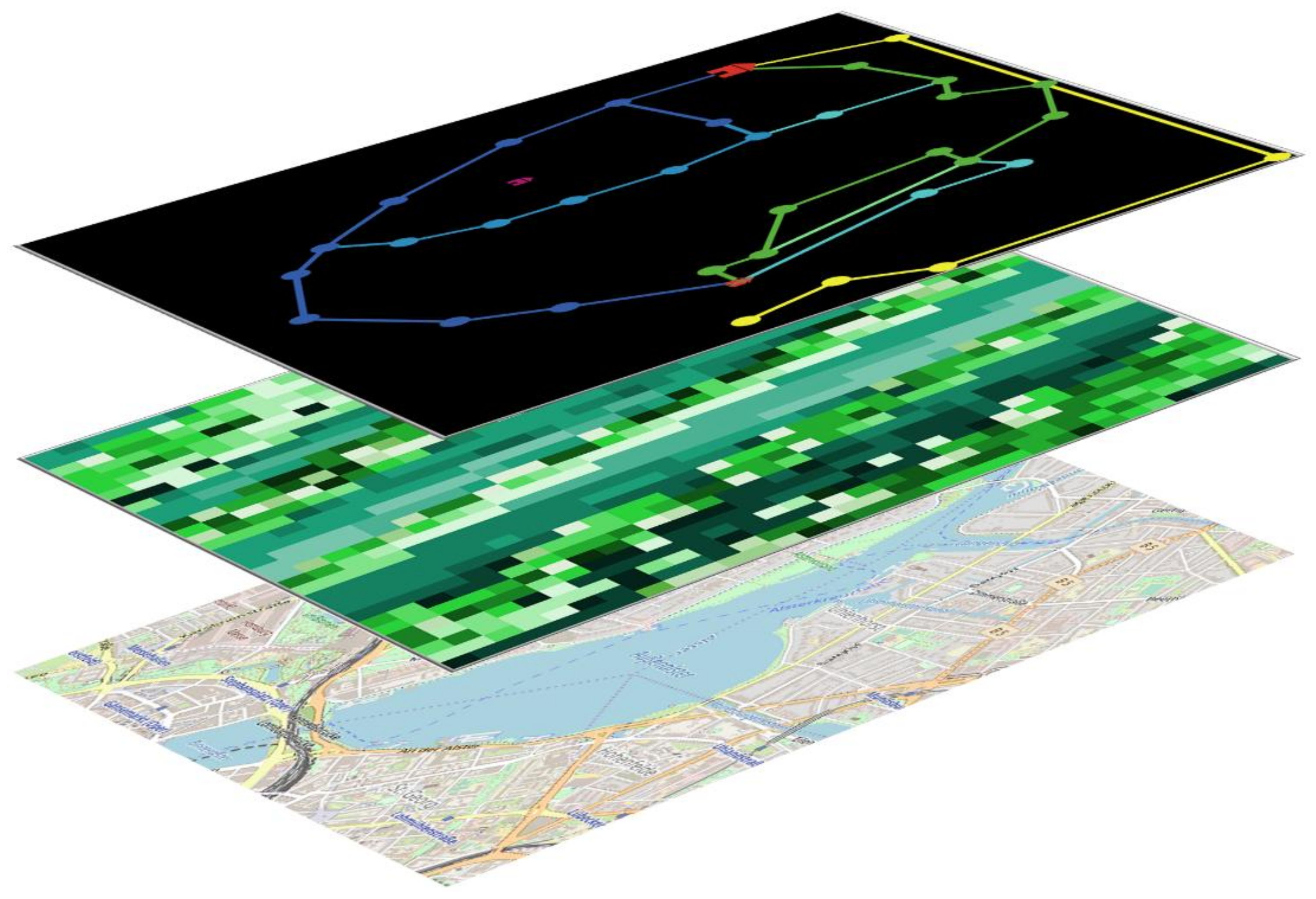
4. A Prototype Application of the ABM Framework to the Case of Hamburg

In order to demonstrate the applicability of the ABM framework, a prototype model implemented in the Netlogo platform is set up for the city of Hamburg to establish essential model components and explore their functioning for the limited data available, leaving a more comprehensive model to further data collection (see the three-level frame in Figure 3). We use the model to simulate the exposure of different kinds of agents who live near the city center to air pollution and thermal stress during their daily commuting to work (Figure 4). At each intersection, agents adapt their path according to the cost, time, and exposure combined in the value function. The different colors represent the means of transport (blue = car, green = bike, yellow = public transport). For car and bike, different routes are possible, and are indicated by the different shades of blue and green (a more detailed description is given in Rühe [68]). In the following, the employed data (Section 4.1), the agent types (Section 4.2), and the model formulation (Section 4.3) are described briefly, and some first results are presented (Section 4.4).

4.1. Data Preparation

In the present model, NO2 concentration data are taken from the chemistry transport model CityChem [60]. The data are averaged separately for the summer and winter of 2012 on a 250 m × 250 m grid. Values for temperature are taken from the German Meteorological Service (DWD) and are randomly set for the same grid using typical ranges for summer (17–24.9 °C) and winter (0–8.9 °C). As soon as long-term high-resolution temperature or heat stress data are available, they can be implemented with the same input routine that was used for the NO2 data. For simplicity, the routes as well as the home and work locations, are predefined (Figure 3 and Table 3). Information about the costs for taking the car were taken from ADAC (Allgemeiner Deutscher Automobil-Club), information about bike costs were available from the Federal Environment Agency (Umweltbundesamt), and the costs for public transportation in Hamburg were from the public transportation service of Hamburg (HVV homepage www.hvv.de). With this information, it was possible to calculate the overall costs for each path.

4.2. Settings of Agents

The agent types are characterized by their different initial priorities for car, bike, and public transport (p1, p2, and p3), their different weights for costs, time, and exposure to environmental stressors (α, β, and γ), the adaptation rate a, and the desired temperature Tdesired (Table 4). The numbers are set for typical urban dwellers based on similar studies in other cities in the literature [69,70,71], with major representative citizen groups (e.g., employee, homemaker, student, wealthy person). This work tries to represent a broader cross-section of society. This is why agent types range from college students with small amounts of money available, with high weights for costs and a high priority for bike transportation, to retired people with low weights for costs and with a high priority for car transportation.

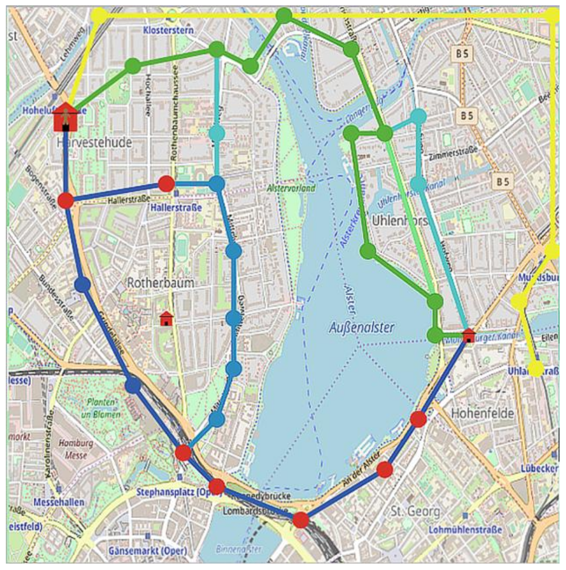
4.3. Performed Simulations

With this prototype model for Hamburg, several model runs were conducted (see Rühe [68]). These include model validation runs with “extreme” agents (e.g., setting α = 1, β = 0, and γ = 0) to test for consistency and plausibility. Here, we select a few model runs to demonstrate the effect of certain scenarios on agent behavior and exposure to validate the framework: (1) a run where rain is randomly turned on for specific times (having an impact on bike usage); and (2) a run where a construction is blocking one road. Finally, a simulation is carried out for which the effect of NO2 on the exposure to environmental stressors in summer and winter is analyzed. This simulation is divided into two runs. The first shows the difference between summer and winter NO2 concentrations and the effect on exposure, and the temperature is constant to only analyze the effect of NO2. In the second run, we analyze the effect of a high temperature, and whether it can compensate for differences in exposure between winter and summer. In the initialization process, the map of Hamburg is loaded, as well as the choosable paths and the datasets on the patches, which are parts of the segmentation of the model world, and are representing the spatial resolution of the data.

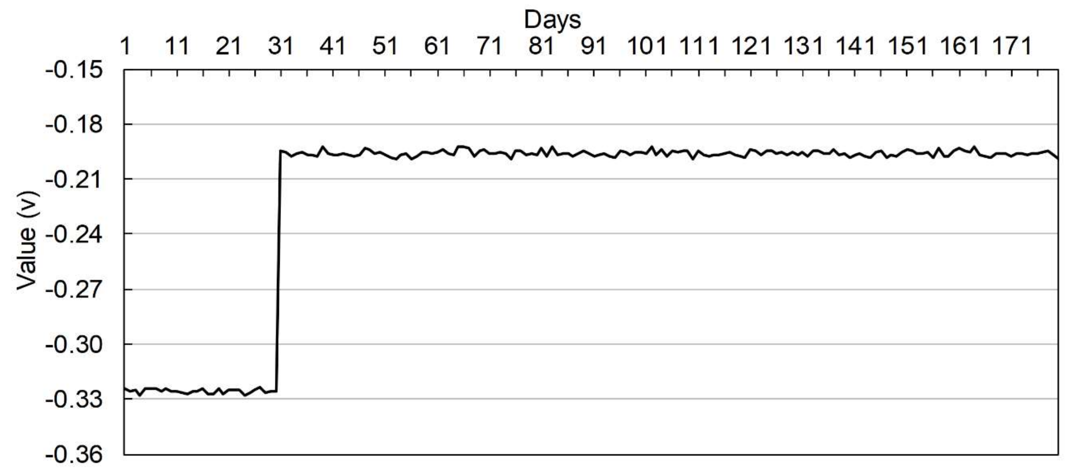
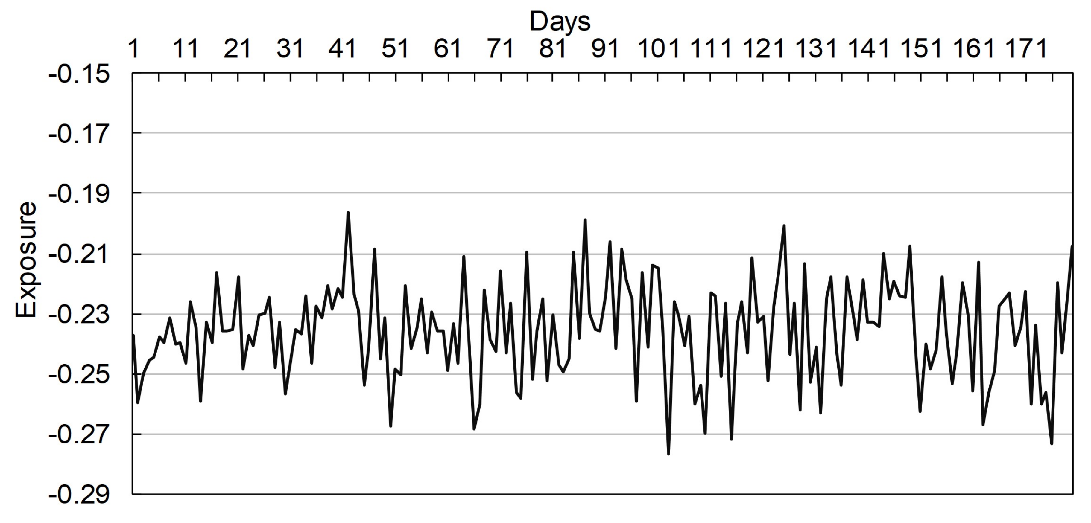
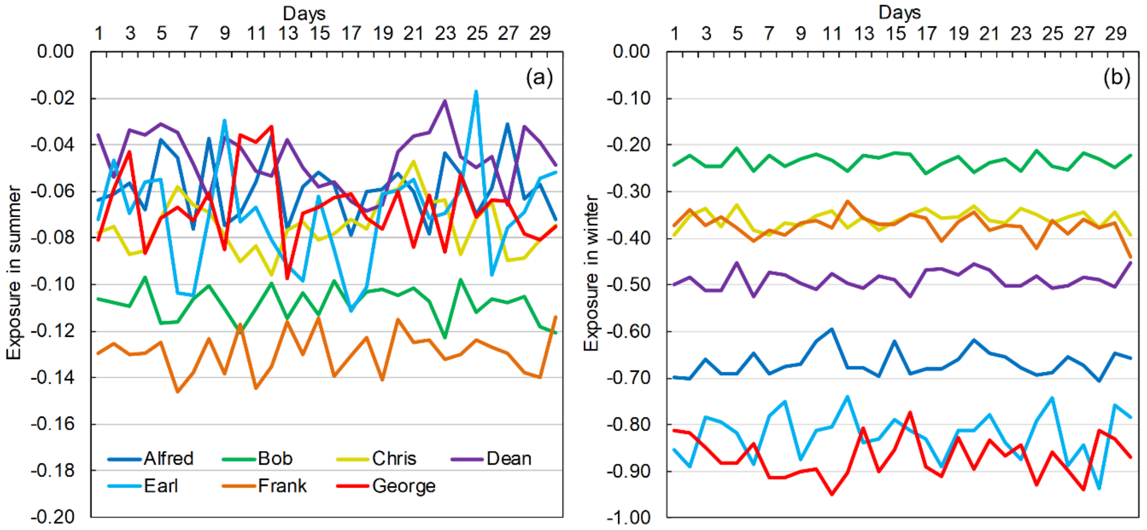
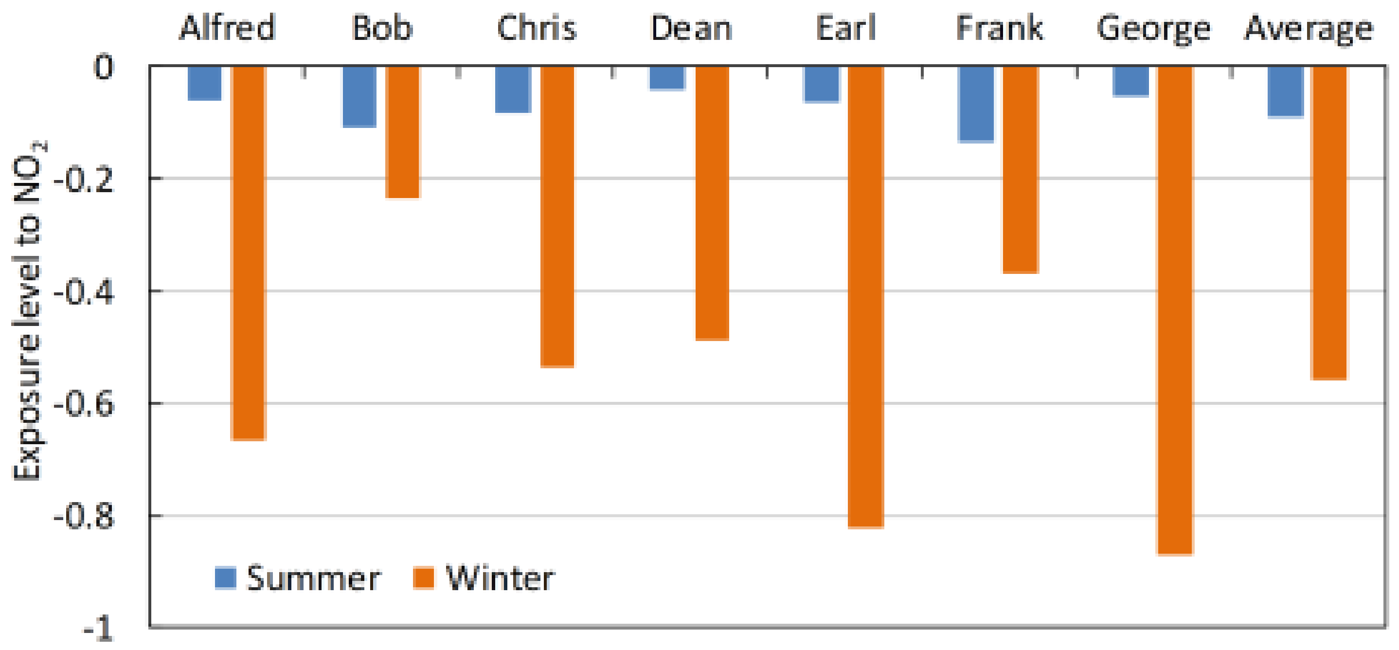
4.4. Preliminary Results

During rain events, bike usage is suppressed in the model. Therefore, agents with a high priority for bike usage (prioritybike) are especially affected by those events. This can be seen in Figure 5 for agent Alfred with initial prioritybike = 0.7. A switch to public transport has a negative effect on the agent’s capital, because costs are much higher for public transport than for a bike (not shown). Agents with a highest priority for cars are not affected by rain events at all.
Construction affects the agents that take their car, as this route is no longer available. For instance, the value v (Equation (2)) of agent Bob, who has a high priority for cars (Table 4), is affected by construction due to the longer commuting time (Figure 6). The exposure variations to environmental stressors do not change noticeably for agent Bob (Figure 7).
Figure 8 shows that there are substantial differences between the exposure of each agent in winter and summer months. It is visible that the exposure in summer months with values between −0.17 and −0.02 is less negative than the exposure in winter months (−0.9 to −0.2). For summer months, data from July 2012 are used, and for winter months, data from January 2012 are used. The exposure data shown in Figure 8 relate only to these two exemplary months. The variations in temperature and NO2-concentration drive the abrupt exposure changes due to individual desired temperatures Tdesired for each agent, as well as the weighting of each term (Table 4). In addition, agents who are using the car decide each day which path they will use. Since concentrations vary strongly in the city (e.g., spots close to water/green areas usually show lower concentrations than roads surrounded by buildings), strong daily variations in exposure to the environmental stressors occur if different paths are chosen. For instance, agent George experiences strong day-to-day variations in exposure, because he reacts to changes in the environmental stressors, and therefore chooses a different path almost each day. His adaptation rate is high (a = 2), and he has a comparably large Tdesired (28 °C). In contrast, agent Bob’s exposure varies only slightly. He solely uses his car due to the large prioritycar (0.95), and the same route because of his low adaptation rate (a = 0.1) and his preference for the fastest route (β = 0.75).
To investigate whether the differences between exposure in summer and winter are due to the differences in NO2 concentration or due to differences in the temperature, additional runs were conducted. In these runs, temperature was kept constant, and only the NO2 concentrations were varied. The differences in the NO2 concentrations between winter and summer have a noticeable effect on the exposure to environmental stressors (not shown). The differences follow the definition of exposure, which is based on an individual desired temperature, e.g., old people prefer other temperatures than young people. Several studies show that NO2 concentrations are higher in winter than in summer [72]; this is mainly caused by more heating processes in winter months. This is also the case in Hamburg. Consequently, Figure 9 shows that for each agent, the average exposure to NO2 is larger in winter than in summer, while the differences between agents are caused by their different behaviors, as was the case for the combined exposure in Figure 8. Summer temperatures would need to reach 42.5 °C in summer in order to experience the same exposure to temperature and NO2 in winter and summer. Based on previous temperature measurements by the DWD, it is very unlikely to reach this value in Hamburg (the highest temperature ever recorded at Hamburg-Fuhlsbüttel was 37.3 °C). To sum it up, even the highest temperatures in Hamburg are not high enough to show the same exposure effect as the high NO2 concentrations in winter months. However, these simulations are idealized, and it is not yet clear how to compare air pollution and heat stress exposure directly, e.g., with respect to health or well-being. Nevertheless, with the proposed ABM, both stressors can be modeled and assessed in a consistent way.

5. Conclusions and Outlooks

This paper presents an agent-based modeling framework for dynamic microsimulations of urban individual exposures to environmental stresses, along with their daily activities in urban areas. Within the framework, decision-making processes are included for each individual based on rule-based behavior to achieve goals under changing environmental conditions. The framework meets the need to develop an innovative and operational approach to understand urban health and well-being that integrates individual characters within a mobility context. Thus, this study helps to integrate substantive considerations of individual well-being into the long-term planning, development, and management of urban environments.
Using the framework for the Hamburg scenario, it is shown that the model framework is flexible enough to handle a variety of input data, as well as extend or replace algorithms. For example, heat stress data from model results could be employed, which will become available in the future. It also shows how the exposure to environmental stressors depends on the agents’ behavior and preferences, because they are able to choose their path through the city, as well as the mode of transport (i.e., car, bike, public transport) according to their individual differences and their complex combinations. The key assumption is that agent decisions are based on commuting costs, time, and the environmental stressors. The exposure to these stressors changes as a result of agent decisions. Consequently, the model already accounts for behavioral changes based on information about air quality, which Koenigstorfer [73] found. The purpose of this case study is not to simulate exact predictions of environmental events, but rather to demonstrate the utility and potential of an agent-based model to be used in an exposure analysis to support environmental incident management. For example, it was shown that the model can be applied to address research questions that are relevant for Hamburg. In the current, very idealized model set-up, lower winter temperatures cannot compensate for the higher NO2 concentrations during this season if the combined exposure to thermal stress and air pollution is of interest.
Moreover, it is very possible to extend the prototype model. Therefore, more algorithms should be added to each package to verify, manipulate, add, or delete data items according to the purpose of the algorithm. Since for each new scenario, different algorithms have to be used or implemented, it is of great interest that algorithms should be separated from the data structure. They also should be easily usable by others. The order in which algorithms are called should be flexible as well. The algorithms are collected into a sub-package of the data structure that they manipulate. Future model extensions will include interactions of multiple agents in traffic, including congestion and traffic jams that force alternative routes and transportation modes, as well as additional environmental exposure from traffic emissions that affect the whole city environment, thus demonstrating the interaction between micro and macro levels.
It has been argued that traditional validation methods are less appropriate for agent-based models, since by their very nature, such models are simplified representations of complex realities, and indicate what may happen rather than what will necessarily happen. This caveat notwithstanding, the validity of this model has been considered in several ways, as illustrated in the modeling framework and implementation sections. Nevertheless, it is only a prototype framework, using basic algorithms that need to be expanded for more real-world conditions and data. Resources are needed to enhance those algorithms and validate the resulting demand against behavioral issues.
While the ABM framework has obvious advantages in comparison to the approaches reviewed in the literature, challenges exist, especially in relation to understanding and quantifying human activities at an individual level. Within the UrbMod project at the University of Hamburg, data from a stakeholder survey with a focus on the daily routines of urban residents in Hamburg and from the patients’ database at the University Hospital Hamburg-Eppendorf are collected [9], which can be applied to set more realistic values for the attributes of agent types and activities. In addition, with respect to heat stress exposure, the individual differences of the agents (e.g., age, gender) and their thermal history (e.g., time spent in sunshine) could be taken into account to model personal dynamic thermal indices, similar to Bruse [74], but for a much larger domain and period. In this way, the adaptive actions of an agent are linked with the thermal history experienced.
The conceptual approach in its current state relies on simplified assumptions and interrelationships between the social and the environmental subsystem, as well as artificial input data. This was necessary, since real data are lacking, and the complexity had to be limited. However, the main objective was to test the feasibility of this approach for exposure assessment, and fully understand the relevant mechanisms that are needed by developing a model prototype. This work also shows the importance of interactions between the transportation community and computer scientists. To satisfy the requirements concerning data management, data processing, computational design and implementation, runtime issues, etc., it is necessary to include computational knowledge into the transportation research process.

Acknowledgments

The authors thank Dejan Antanaskovic for preparation of the data. This work was supported by the research project “Cities in Change-Development of a Multi-sectoral Urban Development-Impact Model (UrbMod; LFF-FV17)”, a joint project of University of Hamburg, Hamburg University of Technology, University Medical Center Hamburg-Eppendorf, Institute of Coastal Research at Helmholtz-Zentrum Geesthacht, Max-Planck-Institute for Meteorology, and HafenCity University, funded by the State of Hamburg. Part of this work is supported through the CliSAP Cluster of Excellence (EXC177), funded by the German Science Foundation (DFG).

Author Contributions

L. Emlyn Yang, Peter Hoffmann and Jürgen Scheffran designed the study; L. Emlyn Yang did the literature overview and constructed the agent-based modeling framework; Sven Rühe performed the prototype modeling and simulation for the Hamburg case; all authors contributed to write the paper.

Conflicts of Interest

The authors declare no conflict of interest.

References

  1. IPCC. Managing the Risks of Extreme Events and Disasters to Advance Climate Change Adaptation. A Special Report of Working Groups I and II of the Intergovernmental Panel on Climate Change; IPCC: Cambridge, UK; New York, NY, USA, 2012; p. 582. [Google Scholar]
  2. Yang, L.; Scheffran, J.; Qin, H.; You, Q. Climate-related flood risks and urban responses in the pearl river delta, china. Reg. Environ. Chang. 2015, 15, 379–391. [Google Scholar] [CrossRef]
  3. Kovats, R.S.; Hajat, S. Heat stress and public health: A critical review. Ann. Rev. Public Health 2008, 29, 41–55. [Google Scholar] [CrossRef] [PubMed]
  4. Lankao, P.R.; Qin, H. Conceptualizing urban vulnerability to global climate and environmental change. Curr. Opin. Environ. Sustain. 2011, 3, 142–149. [Google Scholar] [CrossRef]
  5. Clausen, G.; Wyon, D.P. The combined effects of many different indoor environmental factors on acceptability and office work performance. Hvac&R Res. 2008, 14, 103–113. [Google Scholar]
  6. Bai, X.M.; Nath, I.; Capon, A.; Hasan, N.; Jaron, D. Health and wellbeing in the changing urban environment: Complex challenges, scientific responses, and the way forward. Curr. Opin. Environ. Sustain. 2012, 4, 465–472. [Google Scholar] [CrossRef]
  7. Dias, D.; Tchepel, O. Modelling of human exposure to air pollution in the urban environment: A gps-based approach. Environ. Sci. Pollut. Res. 2014, 21, 3558–3571. [Google Scholar] [CrossRef] [PubMed]
  8. Evance, G. Environmental Stress; Cambridge University Press: Cambridge, UK, 1983. [Google Scholar]
  9. Von Szombathely, M.; Albrecht, M.; Antanaskovic, D.; Augustin, J.; Augustin, M.; Bechtel, B.; Bürk, T.; Fischereit, J.; Grawe, D.; Hoffmann, P. Conceptional modeling approach to health related urban well-being. Urban Sci. 2017, 1, 17. [Google Scholar] [CrossRef]
  10. Schnell, I.; Potchter, O.; Yaakov, Y.; Epstein, Y.; Brener, S.; Hermesh, H. Urban daily life routines and human exposure to environmental discomfort. Environ. Monit. Assess. 2012, 184, 4575–4590. [Google Scholar] [CrossRef] [PubMed]
  11. Rosenzweig, C.; Solecki, W.D.; Hammer, S.A.; Mehrotra, S. Climate Change and Cities: First Assessment Report of the Urban Climate Change Research Network; Cambridge University Press: Cambridge, UK, 2011. [Google Scholar]
  12. Kjellstrom, T.; Friel, S.; Dixon, J.; Corvalan, C.; Rehfuess, E.; Campbell-Lendrum, D.; Gore, F.; Bartram, J. Urban environmental health hazards and health equity. J. Urban Health Bull. N. Y. Acad. Med. 2007, 84, 86–97. [Google Scholar] [CrossRef] [PubMed]
  13. Silva, R.A.; West, J.J.; Zhang, Y.Q.; Anenberg, S.C.; Lamarque, J.F.; Shindell, D.T.; Collins, W.J.; Dalsoren, S.; Faluvegi, G.; Folberth, G. Global premature mortality due to anthropogenic outdoor air pollution and the contribution of past climate change. Environ. Res. Lett. 2013, 8, 034005. [Google Scholar] [CrossRef]
  14. U Nations. World Urbanization Prospects—The 2014 Revision; Department of Economic and Social Affairs: New York, NY, USA, 2014. [Google Scholar]
  15. Chan, M.; Solheim, E.; Taalas, P. Working as one un to address the root environmental causes of ill health. Bull. World Health Org. 2017, 95, 2. [Google Scholar] [CrossRef] [PubMed]
  16. Steinle, S.; Reis, S.; Sabel, C.E. Quantifying human exposure to air pollution-moving from static monitoring to spatio-temporally resolved personal exposure assessment. Sci. Total Environ. 2013, 443, 184–193. [Google Scholar] [CrossRef] [PubMed] [Green Version]
  17. McGeehin, M.A.; Mirabelli, M. The potential impacts of climate variability and change on temperature-related morbidity and mortality in the united states. Environ. Health Perspect. 2001, 109, 185–189. [Google Scholar] [CrossRef] [PubMed]
  18. Watson, A.; Bates, R.; Kennedy, D. Assessment of human exposure to air pollution: Methods, measurements, and models. In Air Pollution, the Automobile, and Public Health; National Academies Press: Washington, DC, USA, 1988. [Google Scholar]
  19. Yang, L.E.; Hoffmann, P.; Scheffran, J. Health impacts of smog pollution: The human dimensions of exposure. Lancet Planet. Health 2017, 1, 132–133. [Google Scholar] [CrossRef]
  20. Willers, S.M.; Jonker, M.F.; Klok, L.; Keuken, M.P.; Odink, J.; van den Elshout, S.; Sabel, C.E.; Mackenbach, J.P.; Burdorf, A. High resolution exposure modelling of heat and air pollution and the impact on mortality. Environ. Int. 2016, 89, 102–109. [Google Scholar] [CrossRef] [PubMed]
  21. Dhondt, S.; Beckx, C.; Degraeuwe, B.; Lefebvre, W.; Kochan, B.; Bellemans, T.; Panis, L.I.; Macharis, C.; Putman, K. Health impact assessment of air pollution using a dynamic exposure profile: Implications for exposure and health impact estimates. Environ. Impact Assess. Rev. 2012, 36, 42–51. [Google Scholar] [CrossRef]
  22. Fryer, M.; Collins, C.D.; Ferrier, H.; Colvile, R.N.; Nieuwenhuijsen, M.J. Human exposure modelling for chemical risk assessment: A review of current approaches and research and policy implications. Environ. Sci. Policy 2006, 9, 261–274. [Google Scholar] [CrossRef]
  23. Gottschalk, F.; Scholz, R.W.; Nowack, B. Probabilistic material flow modeling for assessing the environmental exposure to compounds: Methodology and an application to engineered nano-tio2 particles. Environ. Model. Softw. 2010, 25, 320–332. [Google Scholar] [CrossRef]
  24. Schnell, I.; Potchter, O.; Yaakov, Y.; Epstein, Y. Human exposure to environmental health concern by types of urban environment: The case of tel aviv. Environ. Pollut. 2016, 208, 58–65. [Google Scholar] [CrossRef] [PubMed]
  25. Jerrett, M.; Arain, A.; Kanaroglou, P.; Beckerman, B.; Potoglou, D.; Sahsuvaroglu, T.; Morrison, J.; Giovis, C. A review and evaluation of intraurban air pollution exposure models. J. Expo. Anal. Environ. Epidemiol. 2005, 15, 185–204. [Google Scholar] [CrossRef] [PubMed]
  26. Brauer, M.; Amann, M.; Burnett, R.T.; Cohen, A.; Dentener, F.; Ezzati, M.; Henderson, S.B.; Krzyzanowski, M.; Martin, R.V.; et al. Exposure assessment for estimation of the global burden of disease attributable to outdoor air pollution. Environ. Sci. Technol. 2012, 46, 652–660. [Google Scholar] [CrossRef] [PubMed]
  27. Ragas, A.M.J.; Oldenkamp, R.; Preeker, N.L.; Wernicke, J.; Schlink, U. Cumulative risk assessment of chemical exposures in urban environments. Environ. Int. 2011, 37, 872–881. [Google Scholar] [CrossRef] [PubMed]
  28. Loos, M.; Schipper, A.M.; Schlink, U.; Strebel, K.; Ragas, A.M.J. Receptor-oriented approaches in wildlife and human exposure modelling: A comparative study. Environ. Model. Softw. 2010, 25, 369–382. [Google Scholar] [CrossRef]
  29. CEAM. Multimedia Exposure Assessment Modeling. Epa Center for Exposure Assessment Modeling (ceam). Available online: https://www.Epa.Gov/exposure-assessment-models/multimedia (accessed on 15 April 2018).
  30. CERC. Cambridge environmental research consultants (cerc). In Atmospheric Dispersion Modelling System (adms 5) User Guide, version 5.2; CERC: Cambridge, UK, 2016. [Google Scholar]
  31. Beelen, R.; Raaschou-Nielsen, O.; Stafoggia, M.; Andersen, Z.J.; Weinmayr, G.; Hoffmann, B.; Wolf, K.; Samoli, E.; Fischer, P.; Nieuwenhuijsen, M.; et al. Effects of long-term exposure to air pollution on natural-cause mortality: An analysis of 22 european cohorts within the multicentre escape project. Lancet 2014, 383, 785–795. [Google Scholar] [CrossRef]
  32. Bain, R.; Cronk, R.; Hossain, R.; Bonjour, S.; Onda, K.; Wright, J.; Yang, H.; Slaymaker, T.; Hunter, P.; Prüss-Ustün, A.; et al. Global assessment of exposure to faecal contamination through drinking water based on a systematic review. Trop. Med. Int. Health 2014, 19, 917–927. [Google Scholar] [CrossRef] [PubMed] [Green Version]
  33. Jones, B.; Oneill, B.C.; McDaniel, L.; McGinnis, S.; Mearns, L.O.; Tebaldi, C. Future population exposure to us heat extremes. Nat. Clim. Chang. 2015, 5, 652–655. [Google Scholar] [CrossRef]
  34. Jongman, B.; Ward, P.J.; Aerts, J.C.J.H. Global exposure to river and coastal flooding: Long term trends and changes. Glob. Environ. Chang. 2012, 22, 823–835. [Google Scholar] [CrossRef]
  35. Fuchs, S.; Keiler, M.; Zischg, A. A spatiotemporal multi-hazard exposure assessment based on property data. Nat. Hazard Earth Syst. 2015, 15, 2127–2142. [Google Scholar] [CrossRef] [Green Version]
  36. Hystad, P.; Setton, E.; Cervantes, A.; Poplawski, K.; Deschenes, S.; Brauer, M.; van Donkelaar, A.; Lamsal, L.; Martin, R.; Jerrett, M.; et al. Creating national air pollution models for population exposure assessment in canada. Environ. Health Perspect. 2011, 119, 1123–1129. [Google Scholar] [CrossRef] [PubMed]
  37. Wang, R.; Tao, S.; Balkanski, Y.; Ciais, P.; Boucher, O.; Liu, J.F.; Piao, S.L.; Shen, H.Z.; Vuolo, M.R.; Valari, M.; et al. Exposure to ambient black carbon derived from a unique inventory and high-resolution model. Proc. Natl. Acad. Sci. USA 2014, 111, 2459–2463. [Google Scholar] [CrossRef] [PubMed]
  38. Gulliver, J.; Morley, D.; Vienneau, D.; Fabbri, F.; Bell, M.; Goodman, P.; Beevers, S.; Dajnak, D.; Kelly, F.J.; Fecht, D. Development of an open-source road traffic noise model for exposure assessment. Environ. Model. Softw. 2015, 74, 183–193. [Google Scholar] [CrossRef] [Green Version]
  39. Amirjamshidi, G.; Mostafa, T.S.; Misra, A.; Roorda, M.J. Integrated model for microsimulating vehicle emissions, pollutant dispersion and population exposure. Transp. Res. Part D Transp. Environ. 2013, 18, 16–24. [Google Scholar] [CrossRef]
  40. Hoffmann, P.; Fischereit, J.; Heitmann, S.; Schlünzen, K.H.; Gasser, I. Modeling exposure to heat stress with a simple urban model. Urban Sci. 2018, 2, 9. [Google Scholar] [CrossRef]
  41. ILSI. Ilsi Research Foundation. Cumulative and Aggregate Risk Evaluation System (Cares) Version 4.0. Available online: http://ilsirf.Org/wp-content/uploads/sites/5/2016/08/caresv4overview_install.Pdf (accessed on 15 April 2018).
  42. LifeLine. Overview of the Fundamentals of Version 1.0 of Lifeline—Software for Modeling Aggregate and Cumulative Exposures to Pesticides; The Lifeline™ Project: Manchester, UK, 2000. [Google Scholar]
  43. Liu, H.Y.; Skjetne, E.; Kobernus, M. Mobile phone tracking: In support of modelling traffic-related air pollution contribution to individual exposure and its implications for public health impact assessment. Environ. Health 2013, 12, 93. [Google Scholar] [CrossRef] [PubMed]
  44. Dekoninck, L.; Botteldooren, D.; Panis, L.I.; Hankey, S.; Jain, G.; Karthik, S.; Marshall, J. Applicability of a noise-based model to estimate in-traffic exposure to black carbon and particle number concentrations in different cultures. Environ. Int. 2015, 74, 89–98. [Google Scholar] [CrossRef] [PubMed] [Green Version]
  45. Leyk, S.; Binder, C.R.; Nuckols, J.R. Spatial modeling of personalized exposure dynamics: The case of pesticide use in small-scale agricultural production landscapes of the developing world. Int. J. Health Geogr. 2009, 8, 17. [Google Scholar] [CrossRef] [PubMed] [Green Version]
  46. Kwak, Y.; Park, J.; Arifuzzaman, B.; Iwami, Y.; Amirul, M.; Kondoh, A. Rapid Exposure Assessment of Nationwide River Flood for Disaster Risk Resuction, Proceedings of the XXIII ISPRS Congress, Prague, Czech Republic, 12–19 July 2016; The International Archives of the Photogrammetry, Remote Sensing and Spatial Information Sciences: Prague, Czech Republic, 2016. [Google Scholar]
  47. Neumann, B.; Vafeidis, A.T.; Zimmermann, J.; Nicholls, R.J. Future coastal population growth and exposure to sea-level rise and coastal flooding—A global assessment. PLoS ONE 2015, 10, e0118571. [Google Scholar] [CrossRef] [PubMed]
  48. Christenson, E.; Elliott, M.; Banerjee, O.; Hamrick, L.; Bartram, J. Climate-related hazards: A method for global assessment of urban and rural population exposure to cyclones, droughts, and floods. Int. J. Environ. Res. Public Health 2014, 11, 2169–2192. [Google Scholar] [CrossRef] [PubMed]
  49. Caudeville, J.; Bonnard, R.; Boudet, C.; Denys, S.; Govaert, G.; Cicolella, A. Development of a spatial stochastic multimedia exposure model to assess population exposure at a regional scale. Sci. Total Environ. 2012, 432, 297–308. [Google Scholar] [CrossRef] [PubMed]
  50. Jensen, S.S. Mapping human exposure to traffic air pollution using gis. J. Hazard. Mater. 1998, 61, 385–392. [Google Scholar] [CrossRef]
  51. Gerharz, L.E.; Klemm, O.; Broich, A.V.; Pebesma, E. Spatio-temporal modelling of individual exposure to air pollution and its uncertainty. Atmos. Environ. 2013, 64, 56–65. [Google Scholar] [CrossRef]
  52. Dons, E.; Van Poppel, M.; Panis, L.I.; De Prins, S.; Berghmans, P.; Koppen, G.; Matheeussen, C. Land use regression models as a tool for short, medium and long term exposure to traffic related air pollution. Sci. Total Environ. 2014, 476, 378–386. [Google Scholar] [CrossRef] [PubMed]
  53. Perchoux, C.; Chaix, B.; Cummins, S.; Kestens, Y. Conceptualization and measurement of environmental exposure in epidemiology: Accounting for activity space related to daily mobility. Health Place 2013, 21, 86–93. [Google Scholar] [CrossRef] [PubMed]
  54. An, L. Modeling human decisions in coupled human and natural systems: Review of agent-based models. Ecol. Model. 2012, 229, 25–36. [Google Scholar] [CrossRef]
  55. Bonabeau, E. Agent-based modeling methods and techniques for simulating human systems. PNAS 2002, 99, 7280–7287. [Google Scholar] [CrossRef] [PubMed]
  56. Heppenstall, A.J.; Crooks, A.T.; See, L.M.; Batty, M. Agent-Based Models of Geographical Systems; Springer Science & Business Media: New York, NY, USA, 2011. [Google Scholar]
  57. Langevin, J.; Wen, J.; Gurian, P.L. Simulating the human-building interaction: Development and validation of an agent-based model of office occupant behaviors. Build. Environ. 2015, 88, 27–45. [Google Scholar] [CrossRef]
  58. Monticino, M.; Acevedo, M.; Callicott, B.; Cogdill, T.; Lindquist, C. Coupled human and natural systems: A multi-agent-based approach. Environ. Model. Softw. 2007, 22, 656–663. [Google Scholar] [CrossRef]
  59. An, L.; Lopez-Carr, D. Understanding human decisions in coupled natural and human systems. Ecol. Model. 2012, 229, 1–4. [Google Scholar] [CrossRef]
  60. Karl, M. Development of the city-scale chemistry transport model citychem-episode and its application to the city of hamburg. Geosci. Model Dev. 2018. [Google Scholar] [CrossRef]
  61. Arnfield, A.J. Two decades of urban climate research: A review of turbulence, exchanges of energy and water, and the urban heat island. Int. J. Climatol. 2003, 23, 1–26. [Google Scholar] [CrossRef]
  62. Hoffmann, P.; Krueger, O.; Schlunzen, K.H. A statistical model for the urban heat island and its application to a climate change scenario. Int. J. Climatol. 2012, 32, 1238–1248. [Google Scholar] [CrossRef]
  63. Fischereit, J.; Schlünzen, K.H. Evaluation of thermal indices for their use in obstacle resolving meteorology models. Int. J. Biometeorol. 2018. under review. [Google Scholar]
  64. Hoffmann, P.; Schoetter, R.; Schlünzen, K.H. Statistical-dynamical downscaling of the urban heat island in hamburg, germany. Meteorol. Z. 2016. [Google Scholar] [CrossRef]
  65. Schoetter, R.; Grawe, D.; Hoffmann, P.; Kirschner, P.; Grätz, A.; Schlünzen, K.H. Impacts of local adaptation measures and regional climate change on perceived temperature. Meteorologische Zeitschrift 2013, 22, 117–130. [Google Scholar] [CrossRef]
  66. Federal Environment Agency. Informationsblatt Stickstoffdioxid und Stickstoffoxide—Stand. Available online: https://www.umweltbundesamt.de/sites/default/files/medien/1/dokumente/infoblatt_stickstoffdioxid.pdf (accessed on 10 October 2017).
  67. Scheffran, J.; BenDor, T. Bioenergy and land use: A spatial-agent dynamic model of energy crop production in Illinois. Int. J. Environ. Pollut. 2009, 39, 4–27. [Google Scholar] [CrossRef]
  68. Rühe, S. Simulating Human Exposure to Environmental Stressors in Hamburg: An Agent-Based Model; University of Hamburg: Hamburg, Germany, 2017. [Google Scholar]
  69. Dawson, R.; Peppe, R.; Wang, M. An agent-based model for risk-based flood incident management. Nat. Hazards 2011, 59, 167–189. [Google Scholar] [CrossRef]
  70. Good, N.; Molter, A.; Ackerson, C.; Bachand, A.; Carpenter, T.; Clark, M.L.; Fedak, K.M.; Kayne, A.; Koehler, K.; Moore, B. The fort collins commuter study: Impact of route type and transport mode on personal exposure to multiple air pollutants. J. Expo. Sci. Environ. Epidemiol. 2016, 26, 397–404. [Google Scholar] [CrossRef] [PubMed]
  71. Yang, L.E.; Scheffran, J.; Süsser, D.; Dawson, R.; Chen, Y.D. Assessment of flood losses with household responses: Agent-based simulation in an urban catchment area. Environ. Model. Assess. 2018, 1–20. [Google Scholar] [CrossRef]
  72. Wang, Y.X.; McElroy, M.B.; Martin, R.V.; Streets, D.G.; Zhang, Q.; Fu, T.M. Seasonal variability of nox emissions over east china constrained by satellite observations: Implications for combustion and microbial sources. J. Geophys. Res. Atmos. 2007, 112. [Google Scholar] [CrossRef]
  73. Koenigstorfer, J. Active transportation decision-making against the background of air quality information provision: Walking route preferences of german residents. Urban Sci. 2018, 2, 19. [Google Scholar] [CrossRef]
  74. Bruse, M. Simulating human thermal comfort and resulting usage patterns of urban open spaces with a multi-agent system. In Proceedings of the 24th International Conference on Passive and Low Energy Architecture PLEA, Singapore, 22–24 November 2007; pp. 699–706. [Google Scholar]
Figure 1. Illustration of the agent-based model framework for environmental exposure simulation (adapted and reedited from Leyk et al. [45]).
Urbansci 02 00036 g001
Figure 2. Example of daily routines with priorities p for a female agent who is employed, aged 30–45, and has one child.
Urbansci 02 00036 g002
Figure 3. Three-level structure based on Figure 1, adapted to the model. The first layer below represents the selected research area of the Hamburg map with geographical information (including traffic); the second middle layer shows the environmental stressors (NO2 is shown here); and the third layer presents the traffic network (roads, bike way, rails) and the agents (behavior, characteristics).
Urbansci 02 00036 g003
Figure 4. Map of commuting routes (colors) from home (small red house on the right) to work location (big red house in top left corner), in the prototype model; routes are the same for all of the agents. The third small house represents a day nursery. At each circle, the exposure of the agent is recalculated, implementing the agent-based model (ABM) in NetLogo.
Urbansci 02 00036 g004
Figure 5. Changes in priorityi,k if rain is turned on and off for the agent Alfred. The red ranges are representing the days when the agent is exposed to rain. The y-axes represents the priority for each mode of transportation.
Urbansci 02 00036 g005
Figure 6. Changes in value v if a construction is blocking one route for agent Bob. The x-axes shows the days, and the y-axes show the value function.
Urbansci 02 00036 g006
Figure 7. Changes in exposure to environmental stressors if a construction is blocking one route for agent Bob. The x-axes shows the days, and the y-axes show the exposure differences between winter and summer months.
Urbansci 02 00036 g007
Figure 8. Exposure to environmental stressors (NO2 and temperature variation) in summer (July) (a) and winter months (January) (b) for all agents. Note: the scales of the y-axes in the two figures are different.
Urbansci 02 00036 g008
Figure 9. Individual and average normalized exposures to NO2 for summer and winter.
Urbansci 02 00036 g009
Table 1. Selected sample models in studying human exposure to environmental stressors
CategoryModel PrinciplesExample Models/ApplicationsRepresentative ReferencesModel Features
Modeling of exposure sourcesEstimation of the concentration, distribution, and transportation of exposure sources (pollutants, heat, humidity, radiation, etc.)- Global air pollution (fine particles and ozone) assessmentBrauer et al. [26]- Mainly physical aspects of exposure sources
- Receptors ignored- Suitable in large scale and outdoor exposure
- Result is a map (map set) of stressor concentrations
- Atmospheric Dispersion Modeling System (ADMS 5)CERC, [30]
- Land-use regression (LUR) modelsBeelen et al. [31]
- Multimedia exposure assessment modelingCEAM, [29]
- Water quality regression modelBain et al. [32]
- Indicator-based heat and air pollution combinationWillers et al. [20]
- Scenario projections from regional climate modelsJones et al. [33]
Modeling or assessment of exposed population- Assess the population or area or property that is exposed to certain stressor concentrations
- Compare the exposure status/level of sub-regions or sub-group of the population
- Modeling exposure to natural hazards such as flooding, cyclone, droughtsJongman et al. [34];
Fuchs et al. [35]
- Offer an overview of group exposure
- Produce relative comparison of sub-group’s exposures
- Suitable in large scale and outdoor exposure
- Result is a population or area associated with certain stressor concentration (population-weighted concentrations)
- Global and regional human exposures to air pollutionsHystad et al. [36];
Wang et al. [37]
- Noise exposure modelGulliver et al. [38]
- Traffic noise and pollution exposure modelAmirjamshidi et al. [39]
- Heat stress exposure model in combination with traffic modelHoffmann et al. [40]
Modeling of individual’s exposure degree- Assess the accumulation of exposure at a series of times and locations
- Simulate the exposure degree of specific receptors
- Mostly adopted with receptors’ mobility and activity
- Cumulative and Aggregate Risk Evaluation System (CARES)ILSI, [41]- Focus on sampled individual receptors
- Suitable to model multiple stressors
- Limited number of receptors
- Specific and accurate at individual level
- Result is an integrative degree/intensity of a subject being exposed (time-weighted concentrations)
- Lifeline (exposure to pesticide)LifeLine, [42]
- Mobile-tracked traffic-related air pollution modelLiu et al. [43]
- Urban exposure in daily life routinesSchnell et al. [24]
Schnell et al. [10]
- GPS-based modeling of urban exposure to air pollutionDias and Tchepel, [7]
- Modeling exposure to multiple stressorsDekoninck et al. [44]
- Personalized model of pesticide use Leyk et al. [45]
Table 2. Example of agents’ attributes, behaviors, and agent groups with different daily activities (no relation between the columns).
AttributesBehaviorsAgent groups
AgeWorking G1: worker, 18–30 years old, single, cycling, living in apartment older than 1980, shopping once a week
Gender Shopping
EmploymentChild caringG2: homemaker, 30–45 years old, married with children, using private car, living in suburban house, shopping daily
Living locationEntertaining
Work locationSleepingG3: worker, 45–65 years old, children independent, using mixed transportations
Traffic typeTraveling
Building typePreventing G4: retired couple, living in suburban house, using public transportation, shopping once a week
Regular runnerRunning/jogging
Table 3. Time, length, and costs for the different routes shown in Figure 4.
Car1Car2Car3Car4Car5BikePublic
Time [min]10161715131918
Length [km]5.15.36.87.16.65.06.3
Costs [€]1.531.592.042.131.980.41.07
Table 4. Attribute rs of different agents.
Agent TypeAlfredBobChrisDeanEarlFrankGeorge
Initial prioritycar0.10.950.650.3330.10.3330.8
Initial prioritybike0.70.0250.0010.3330.20.3330.1
Initial prioritypublic0.20.0250.34990.3330.70.3330.1
Adaptation rate (a)100.11.230.142
Weighting factor for costs (α)0.60.050.30.10.450.80.8
Weighting factor for time (β)0.10.750.10.70.450.10.1
Weighting factor for exposure to environmental stressors (γ)0.30.20.60.20.10.10.1
Desired temperature Tdesired [°C]23182123231928

