The Relationship between Land Cover and Sociodemographic Factors


1
Department of City & Metropolitan Planning, University of Utah, Salt Lake City, UT 84112, USA
2
Department of Atmospheric Sciences, University of Utah, Salt Lake City, UT 84112, USA
3
Division of Pulmonary Medicine, School of Medicine, University of Utah, Salt Lake City, UT 84132, USA
4
NEXUS Institute, University of Utah, Salt Lake City, UT 84112, USA
Urban Sci. 2020, 4(4), 68; https://0-doi-org.brum.beds.ac.uk/10.3390/urbansci4040068
Submission received: 31 October 2020
/
Revised: 1 December 2020
/
Accepted: 1 December 2020
/
Published: 2 December 2020
(This article belongs to the Special Issue Urban Health: Emission Sources, Pollutant Transport, and Associated Health Impacts)
Abstract
:Multiple social and environmental justice concerns are linked to the urban form such as the distribution of socioeconomic class populations, healthcare spending, air pollution exposure, and human mobility. Because of this, the implications of the relationships between built urban form, sociodemographic factors, and air quality warrant analysis at a high spatial resolution. This study used 1m resolved LiDAR data to characterize land use in Salt Lake County, Utah, and associate it with sociodemographic and air quality data at the census block group and zip code levels. We found that increasing tree cover was associated with higher per capita income and lower minority populations while increasing built cover was linked to lower per capita income and higher minority populations. Air quality showed less strong correlations, however, decreased non-irrigated cover, increased built cover, and higher amounts of households living under poverty were related to higher long-term PM2.5 exposure. Due to regional air pollution concerns, several policy efforts have been undertaken to improve air quality and reduce negative health outcomes in Utah which are being informed by regulatory and research-grade air quality sensors.
1. Introduction
Land cover at the urban level has often been studied using LiDAR data due to its thoroughness and availability [1,2]. The urban form influences behavior ranging from transit use [3] to how children go to school [4]. Increased tree cover has been shown to promote healthier communities with highly-built areas showing the opposite effect [5,6,7]. As cities continue to increase in spatial extent and population, there is a growing need to better characterize urban emissions, particularly of criteria air pollutants (CAPs) for metropolitan planning [8,9], health [10], and emissions reduction purposes, from global to local scales [11,12].
Multiple social and environmental justice concerns are linked to the urban form such as the distribution of socioeconomic class populations [13], healthcare spending [14], and human mobility [15]. Urban areas composed of lower socioeconomic populations are disproportionately affected by hotter temperatures [16] which has been shown to have adverse health impacts [17,18,19]. Furthermore, land cover disparities have been associated with air pollution [20] and several health outcomes [21] including asthma hospitalizations [22].
The need for a thorough analysis of the implications of urban ecology on social justice using remote sensing tools, including LiDAR, has been highlighted in the literature [23]. While the relationship between urban tree cover and political economics is well-established [24], a remaining knowledge gap is the lack of studies linking land use, sociodemographic characteristics, and air pollution. Previous work has used LiDAR data to identify and classify urban land cover, with granular analyses performed at the parcel level [25,26]. Highly-resolved LiDAR was used to compare tree biomass and sociodemographic characteristics in Boston [27], but no significant differences were found across these variables, primarily because tree cover variability was unrelated to wealth, minority population, or education level. However, other studies, using similar approaches, found distinct tree cover differences along sociodemographic lines in Miami-Dade County [28,29], Milwaukee [30], and Santiago de Chile [31]. These studies showed that areas with higher-percent minority populations had lower amounts of tree cover and green spaces; these socioeconomic determinants can be used as a predictor of green space as yards in private residences [32] and urban forestry [33].
The relationship between air pollution and land cover has been studied extensively [34,35], with potential exposure quantified [36] and associated with health outcomes, including asthma hospitalizations [22]. However, outside of population or population density, little attention has been paid to other sociodemographic determinants including race or income. Many of these studies used land regression techniques to estimate emissions [37], but none relied on a dense air quality observation network to more accurately quantify potential exposure.
In the present study, we combined a 1m land cover dataset with sociodemographic variables and air pollution measurements to show their linkages. While previous studies have focused on one or two of these aspects, this study linked these three variables to encourage a more comprehensive approach to understanding intrinsic neighborhood-level differences. This analysis, performed at the census block group and zip code level, facilitates localized policy actions by identifying areas of greatest disparity at fine resolution. This is the first use of the highly resolved LiDAR data product developed for Salt Lake County and will set a precedent for future land cover analyses to incorporate all three components—namely land use, sociodemographics, and air pollution—for the public health policy purposes.
2. Materials and Methods
2.1. Land Use Data
Five land cover classes were mapped for the urban extent of Salt Lake County (approximately 840 km2) using two high spatial resolution datasets. Four-band, 1m resolution orthoimagery was collected under the National Agriculture Imagery Program (NAIP) in summer 2014. Orthoimage brightness values were used to calculate the normalized difference vegetation index [38], green-red vegetation index [39,40], and metrics of spatial variability of each band and index. First return, last return, and bare earth digital surface models derived from LiDAR data collected in late 2013 and early 2014 were resampled from their original 0.5m resolution to match the 1m resolution of the orthoimagery. The surface models were differenced, and metrics of spatial variability were also calculated. Orthoimage and LiDAR variables were extracted from polygons for deciduous trees, coniferous trees, irrigated low-stature vegetation, non-irrigated vegetation/soil, and impervious surface/water classes and then used to train a random forests classifier [41]. Classification results were assessed using an independent set of polygons and yielded an overall accuracy of 96.2% and a 0.94 kappa value [42]. The land cover categories are listed in Table 1.
2.2. Sociodemographic Data
Zip-code-level sociodemographic data were retrieved from the Healthy Salt Lake dataset [43], and census block group data were obtained from the United States Census Bureau American Community Survey [44]. The relevant data fields extracted were Percent Minority Population, Per Capita Income, and Percentage of Households Living Below Poverty. The shapefiles for each dataset provided centroid latitude and longitude coordinates. Salt Lake County has 612 block groups, and 34 zip codes were used in this analysis.
2.3. Air Pollution Data
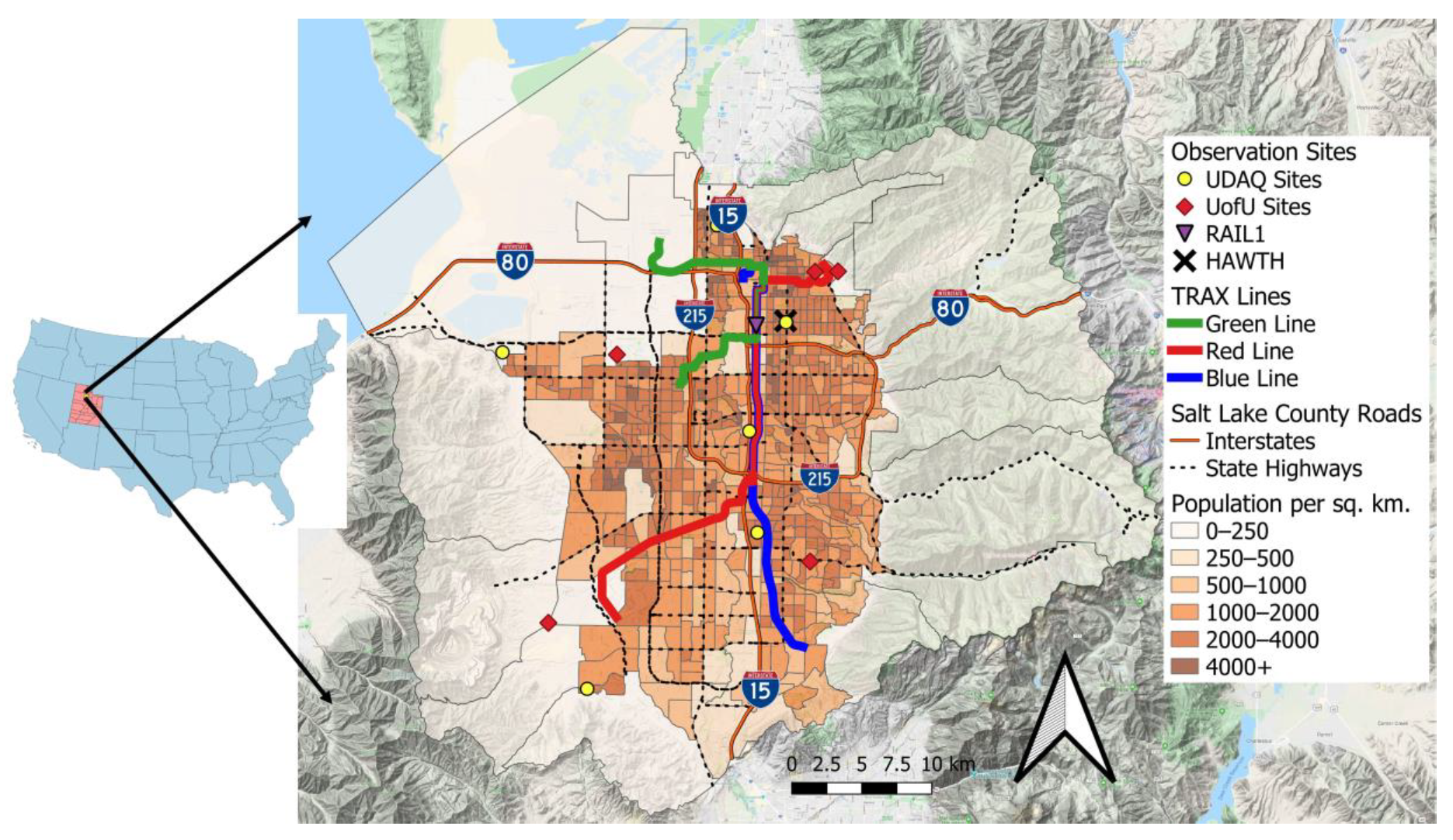
Salt Lake County area is home to a dense criteria air pollution observational network facilitating a wide range of observation studies [45,46,47]. We used data from the Utah Division of Air Quality (UDAQ) regulatory observational network and the University of Utah (UofU) stationary and mobile platform network. The mobile network consists of air quality sensors that measure fine particulate matter (PM2.5) and ozone [48,49] mounted on top of electric Utah Transit Authority (UTA) light-rail (TRAX) trains (Figure 1). We estimated mean PM2.5 concentrations for three years (2017–2019) at each zip code’s centroid using the inverse distance square weighting (IDW) method [50,51] applied to data from the complete air pollution observation network.
2.4. Geographical and Sociodemographic Comparisons
The 1m land use cover data were intersected with the zip code and block group shapefiles to calculate areal land cover by category using QGIS version 3.14.15. These values were converted to percent land cover at each geographical resolution. In this study, coniferous and deciduous trees were combined to form the “Tree” category. Similarly, low impervious surface and roof were combined into the “Built” category. A linear model was used to compare the different land use, sociodemographic, and pollution variables.
3. Results
3.1. Geographical Distribution of Land Cover Categories
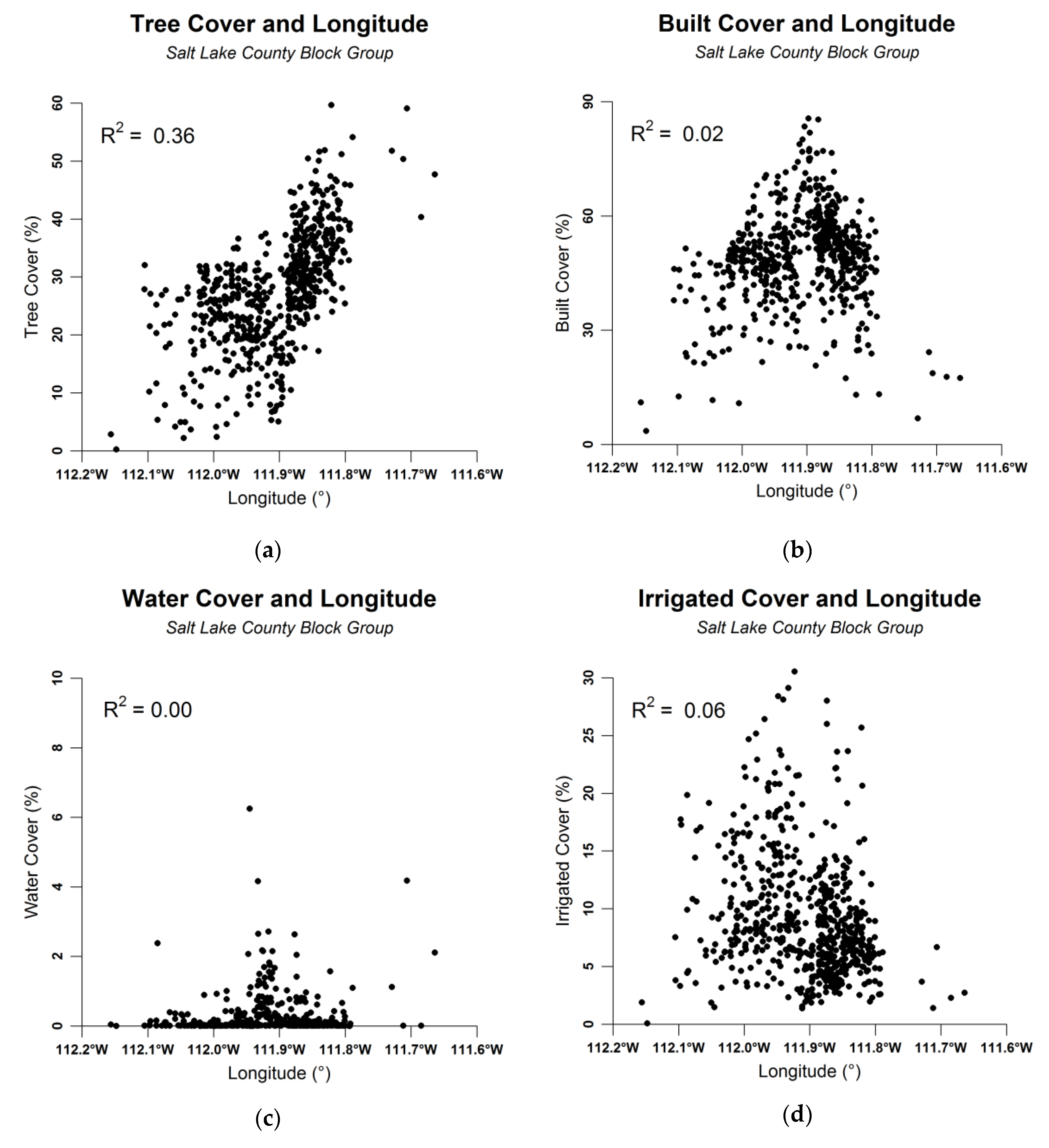
Salt Lake County has a marked East-West sociodemographic divide demarcated by U.S. Interstate 15 which runs North-South (Figure 1). The West Side is developing at a rapid pace and is home to a higher-percent minority and lower-income population. The land cover implications of these differences are shown in Figure 2, along with R2 values using a linear fit. Figure 2a clearly demonstrates the longitudinal distribution of tree cover, with the older and wealthier East Side home to more trees. The built cover (Figure 2b) is highest in the central part of the county as this is the commercial and industrial center along Interstate 15. The built cover drops rapidly on the East Side and is comparatively higher on the West Side due to the siting of factories and commercial buildings in that part of the county. The distribution of water is relatively constant with the exception of the Jordan River which runs near to the center of the county (Figure 2c). Lastly, irrigated cover is highly concentrated in the central part of the county as it generally belongs to commercial and institutional buildings, as well as homes, and is less present on the East Side (Figure 2d).
3.2. Sociodemographic Distribution of Land Cover Categories
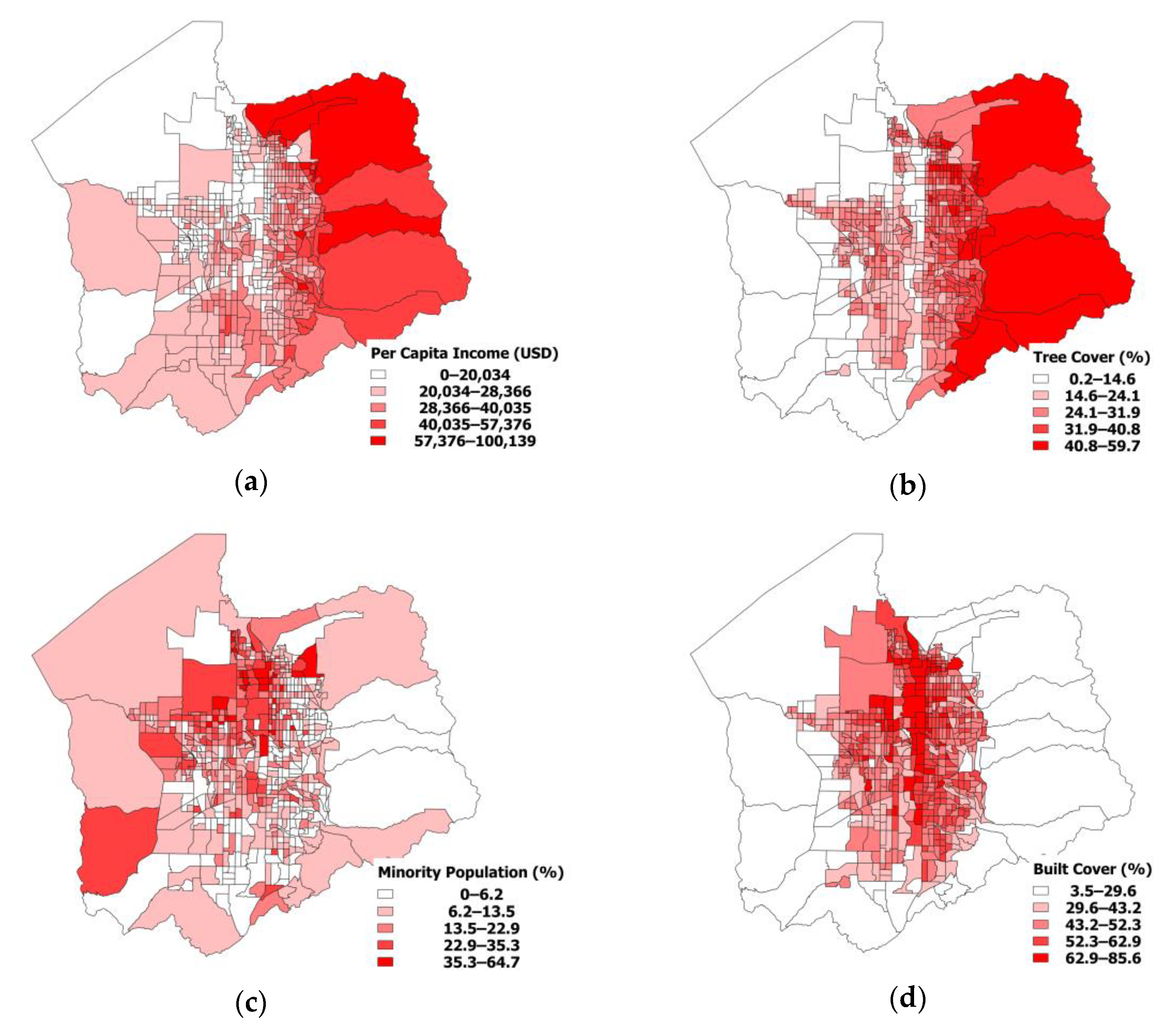
Spatially-resolved sociodemographic variables and land cover categories are shown in Figure 3. The more affluent East Side is clearly highlighted in Figure 3a with only one census block group west of I-15 having an average per capita income of over USD 40,035/yr, and the majority averaging less than USD 28,366/yr. The tree cover (Figure 3b) displays a similar pattern, with few census block groups west of I-15 having over 31.9% of tree cover and most averaging less than 24.1% tree cover. The minority population is most concentrated in the northwest part of the county (Figure 3c) reaching values as high as 64.7%, with the east side of the county generally having less than 13.5% minority population. The built cover is highest in the central part of the county and along the I-15 and I-80 highways (Figure 3d). The spatial distribution pattern consistently follows the population density map shown in Figure 1.
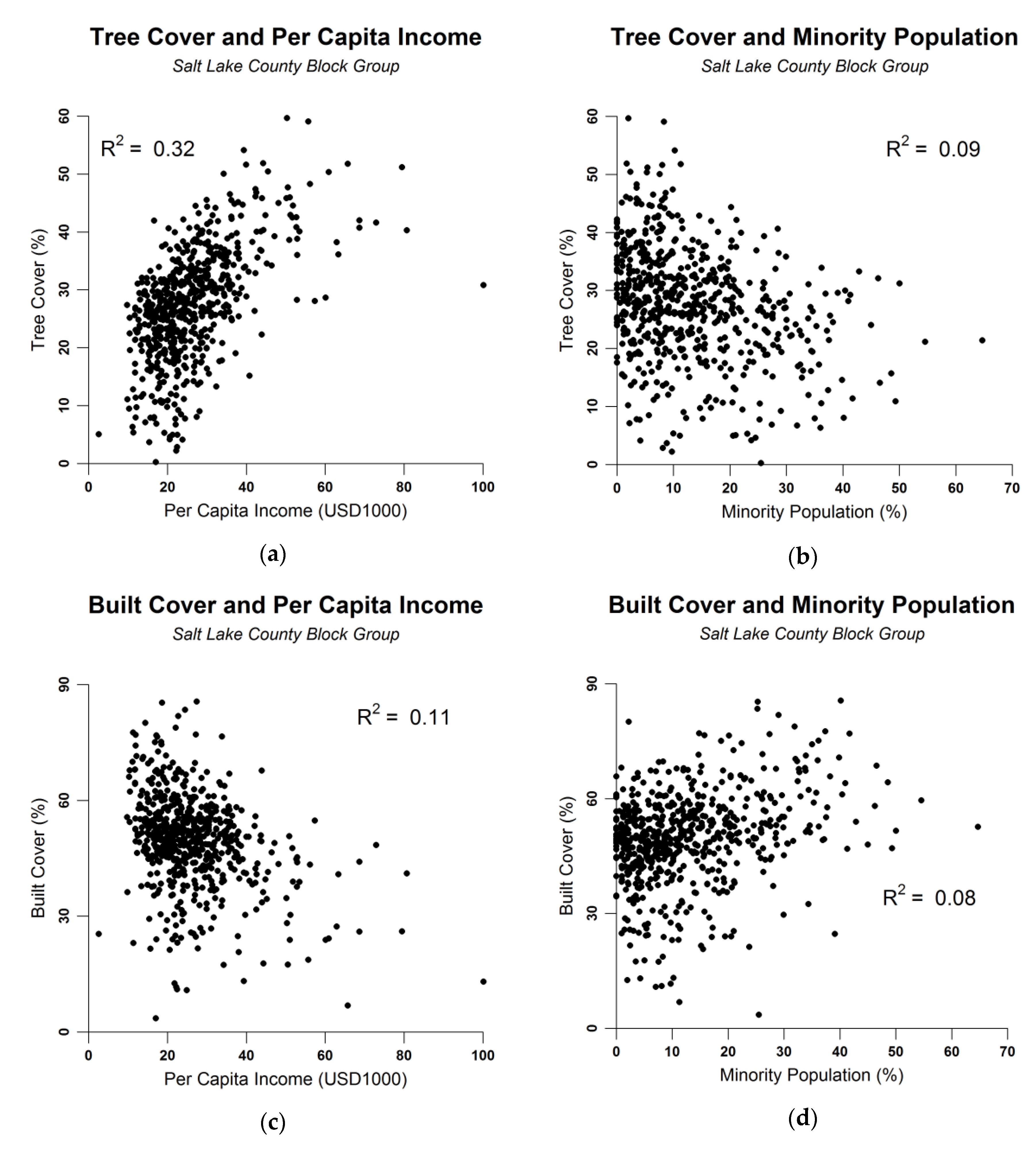
Figure 4 shows relationships between sociodemographic variables and land cover, along with R2 values using a linear fit. Tree cover increases with increasing per capita income at the census block group as seen in Figure 4a, however, it decreases with an increasing minority population (Figure 4b). The built environment displays the opposite pattern with decreasing cover associated with higher per capita income (Figure 4c) and increasing cover related to a higher minority population (Figure 4d).
Tree cover and per capita income (Figure 4a) show the strongest association of the four comparisons depicted in this analysis. It can be surmised that higher-income populations are able to afford to either own property with a proportionately larger amount of trees (either by living near an untouched forest or growing trees on their property) or invest in neighborhood park development. Built cover (Figure 4c,d) shows less strong associations with income and minority populations because the central areas contain both higher-cost and more affordable living spaces. Furthermore, a low amount of built cover can be associated with either a more undeveloped rural location on the fringes of the county or an area with a large amount of purposely placed trees.
3.3. Long-Term PM2.5 Concentrations and Land Cover and Household Poverty
The relationships between fine particulate matter concentrations at zip code centroids and study variables are shown in Figure 5, along with R2 values using a linear fit. Higher long-term pollutant concentrations are associated with increasing built cover (Figure 5a) and lower concentrations are linked with increasing non-irrigated cover (Figure 5b). There is no clearly visible relationship between PM2.5 concentrations and tree cover (Figure 5c). A comparatively weaker association between increased pollutant concentrations and percent of households living below poverty is shown in Figure 5d.
4. Discussion
The geographical distribution of land cover in Salt Lake County shown in Figure 1 demonstrates the natural and built environment. The Jordan River is a major body of water and runs North-South in the center of the county. The East Side of the county is more mature and composed of more green spaces, including parks, and thus has had more time to develop urban forests. The built and irrigated areas are centrally located because that is where commercial and institutional buildings are found. The irrigated areas correspond to lawns and low shrubs, commonly associated with commercial and some residential buildings.
The relationships between land cover and sociodemographic variables shown in Figure 4 demonstrate a well-established and known pattern that links wealthier and lower-minority areas with larger amounts of green space. This finding is akin to results from the existing literature [32,33]. Conversely, lower-income and higher-minority areas generally have a higher fraction of its surface as built cover. However, these associations are not strong, nor statistically significant, echoing findings from previous studies [27]. A visual representation of the East-West divide is shown in Appendix A, Figure A1.
Localized air pollution is generally most strongly linked to nearby emission sources compared to transport from outside sources. The built environment is associated with both mobile (vehicle) and stationary (buildings, industrial, etc.) sources. Therefore, the relationship between increased pollution and increased built cover (Figure 5) is to be expected as has been found in multiple studies [48,52,53]. Non-irrigated cover refers to untouched land cover and is inversely proportional to built cover, thus showing the opposite pattern. Tree cover is either urban forest or undisturbed natural forest. The urban forests are generally located in areas that have higher pollution due to being in more built-up areas while undisturbed forests tend to be on the edges of cities and would be associated with less pollution. Elevated periods of PM2.5 are generally found in the winter when most trees are generally inactive thus reducing their ability to filter pollutants. However, with increased incidences of wildfires, particularly in the summer when trees generally have their full array of leaves, vegetation may prove to be a more important factor in ameliorating air quality concerns. Finally, while the relationship is less obvious, deeply impoverished areas may be more impacted by higher levels of pollution.
5. Conclusions
This study used 1m resolved LiDAR data to characterize land use in Salt Lake County, Utah, and associated it with sociodemographic and air quality data. This highly resolved data product allowed comparisons at the census block group and zip code level. We found that increasing tree cover was associated with higher per capita income and lower minority populations while increasing built cover was linked to lower per capita income and higher minority populations. Air quality showed less strong correlations, however, decreased non-irrigated cover, increased built cover, and higher amounts of households living under poverty were related to higher long-term PM2.5 exposure.
The findings from this work highlight glaring differences in terms of land cover and potential air pollution exposure spatially distributed along sociodemographic lines. These disparities have been analyzed separately in the past, but this manuscript combines a detailed comparison using all three variable groups showing there are several non-negligible associations between them. This methodology facilitates an understanding of the implications of land use, particularly urban forests, with regards to air pollution. Thus, the effects of reducing pollution emitters may not be felt equally across an area since tree and built cover are likely to have an impact on potential pollution exposure. Therefore, efforts to mitigate air pollution should consider involving land cover as part of a more holistic approach, the effects of which are likely to be felt most strongly by populations spending large amounts of time outdoors [54].
Several positive advances in air quality monitoring and legislative efforts have already taken place in Utah. The TRAX Light-Rail Train Air Quality Observation Project [49] has been monitoring air quality across Salt Lake County since 2015 providing unprecedented spatial and temporal resolution. Air quality data from this project was used in a recent study associating air pollution with school absences [55]. These findings resulted in the 2019 Utah State Legislature passing Rep. Wheatley’s HB 0344 “Student Asthma Relief Amendments” [56] which provides stock inhalers (albuterol) to all schools in the state. Based on research showing how the local mass transit system is a valuable tool in reducing air pollutants [57], Rep. Briscoe successfully passed HB 0353 “Reduction of Single Occupancy Vehicle Trips Pilot Program” providing free transit fares on poor air quality days to encourage ridership [58]. Additionally, in an effort to better quantify the environmental impacts of new developments, Sen. Luz Escamilla passed SB 0112 “Inland Port Amendments” [59].
Future work will increase the resolution of air quality observations—both temporally (seasonally) and spatially (census block group level). The health impacts of poor air quality have been well-studied, both in Salt Lake County and elsewhere, however, the link between urban form and health, particularly at high resolution, needs further development. The Wasatch Front Regional Council, the region’s Metropolitan Planning Agency, has produced projected land use scenarios [60] which will be analyzed to understand implications for environmental justice as well as potential air quality and health impacts.
Funding
This research received no external funding.
Acknowledgments
Phil Dennison, Department of Geography, University of Utah.
Conflicts of Interest
The author declares no conflict of interest.
Appendix A
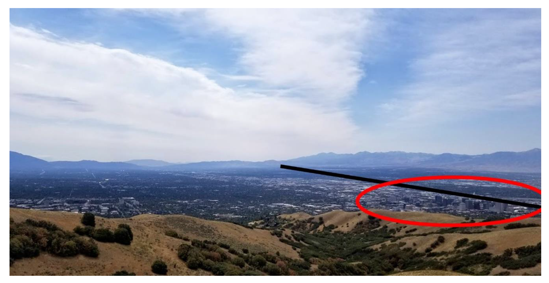
The geographical land cover layout of Salt Lake County can be observed in Figure A1. The East Side of the county, to the left of the dividing black line, is more mature and has a higher fraction of green areas, while the West Side of the county, to the right of the dividing black line, is developing quickly and has less green areas due to a higher fraction of industrial and commercial buildings. The downtown area (red oval) is highly built up and has few green areas outside of two parks.
Figure A1.
Southwest-facing view of Salt Lake County. The red oval shows the downtown area, and the black line aligns with U.S. Interstate 15 separating the East Side (left) from the West Side (right).
Figure A1.
Southwest-facing view of Salt Lake County. The red oval shows the downtown area, and the black line aligns with U.S. Interstate 15 separating the East Side (left) from the West Side (right).

References
- Yan, W.Y.; Shaker, A.; El-Ashmawy, N. Urban land cover classification using airborne LiDAR data: A review. Remote Sens. Environ. 2015, 158, 295–310. [Google Scholar] [CrossRef]
- Wang, K.; Wang, T.; Liu, X. A review: Individual tree species classification using integrated airborne LiDAR and optical imagery with a focus on the urban environment. Forests 2019, 10, 1. [Google Scholar] [CrossRef] [Green Version]
- Crane, R. The influence of urban form on travel: An interpretive review. J. Plan. Lit. 2000, 15, 3–23. [Google Scholar] [CrossRef]
- Larsen, K.; Gilliland, J.; Hess, P.; Tucker, P.; Irwin, J.; He, M. The influence of the physical environment and sociodemographic characteristics on children’s mode of travel to and from school. Am. J. Public Health 2009, 99, 520–526. [Google Scholar] [CrossRef]
- Nowak, D.J.; Hirabayashi, S.; Bodine, A.; Greenfield, E. Tree and forest effects on air quality and human health in the United States. Environ. Pollut. 2014, 193, 119–129. [Google Scholar] [CrossRef] [Green Version]
- Tsai, W.-L.; Leung, Y.-F.; McHale, M.R.; Floyd, M.F.; Reich, B.J. Relationships between urban green land cover and human health at different spatial resolutions. Urban Ecosyst. 2019, 22, 315–324. [Google Scholar] [CrossRef]
- Carpio, O.; Fath, B. Assessing the environmental impacts of urban growth using land use/land cover, water quality and health indicators: A case study of Arequipa, Peru. Am. J. Environ. Sci. 2011, 7, 90–101. [Google Scholar] [CrossRef] [Green Version]
- Gurney, K.R.; Romero-Lankao, P.; Seto, K.C.; Hutyra, L.R.; Duren, R.; Kennedy, C.; Grimm, N.B.; Ehleringer, J.R.; Marcotullio, P.; Hughes, S. Climate change: Track urban emissions on a human scale. Nature 2015, 525, 179. [Google Scholar] [CrossRef] [Green Version]
- Parshall, L.; Gurney, K.; Hammer, S.A.; Mendoza, D.; Zhou, Y.; Geethakumar, S. Modeling energy consumption and CO2 emissions at the urban scale: Methodological challenges and insights from the United States. Energy Policy 2009, 38, 4765–4782. [Google Scholar] [CrossRef]
- Markakis, K.; Poupkou, A.; Melas, D.; Tzoumaka, P.; Petrakakis, M. A Computational Approach Based on GIS Technology for the Development of an Anthropogenic Emission Inventory of Gaseous Pollutants in Greece. Water Air Soil Pollut. 2010, 207, 157–180. [Google Scholar] [CrossRef]
- Asefi-Najafabady, S.; Rayner, P.J.; Gurney, K.R.; McRobert, A.; Song, Y.; Coltin, K.; Huang, J.; Elvidge, C.; Baugh, K. A multiyear, global gridded fossil fuel CO2 emission data product: Evaluation and analysis of results. J. Geophys. Res. Atmos. 2014, 119, 10213–10231. [Google Scholar] [CrossRef] [Green Version]
- Hutyra, L.R.; Duren, R.; Gurney, K.R.; Grimm, N.; Kort, E.A.; Larson, E.; Shrestha, G. Urbanization and the carbon cycle: Current capabilities and research outlook from the natural sciences perspective. Earth’s Future 2014, 2, 473–495. [Google Scholar] [CrossRef] [Green Version]
- Avelar, S.; Zah, R.; Tavares-Corrêa, C. Linking socioeconomic classes and land cover data in Lima, Peru: Assessment through the application of remote sensing and GIS. Int. J. Appl. Earth Obs. Geoinf. 2009, 11, 27–37. [Google Scholar] [CrossRef]
- Becker, D.A.; Browning, M.H.; Kuo, M.; Van Den Eeden, S.K. Is green land cover associated with less health care spending? Promising findings from county-level Medicare spending in the continental United States. Urban For. Urban Green. 2019, 41, 39–47. [Google Scholar] [CrossRef]
- Lenormand, M.; Louail, T.; Cantú-Ros, O.G.; Picornell, M.; Herranz, R.; Arias, J.M.; Barthelemy, M.; San Miguel, M.; Ramasco, J.J. Influence of sociodemographic characteristics on human mobility. Sci. Rep. 2015, 5, 10075. [Google Scholar] [CrossRef] [Green Version]
- Mitchell, B.C.; Chakraborty, J. Landscapes of thermal inequity: Disproportionate exposure to urban heat in the three largest US cities. Environ. Res. Lett. 2015, 10, 115005. [Google Scholar] [CrossRef] [Green Version]
- Rosenthal, J.K.; Kinney, P.L.; Metzger, K.B. Intra-urban vulnerability to heat-related mortality in New York City, 1997–2006. Health Place 2014, 30, 45–60. [Google Scholar] [CrossRef] [Green Version]
- Wong, K.V.; Paddon, A.; Jimenez, A. Review of world urban heat islands: Many linked to increased mortality. J. Energy Resour. Technol. 2013, 135, 022101. [Google Scholar] [CrossRef]
- Schinasi, L.H.; Benmarhnia, T.; De Roos, A.J. Modification of the association between high ambient temperature and health by urban microclimate indicators: A systematic review and meta-analysis. Environ. Res. 2018, 161, 168–180. [Google Scholar] [CrossRef]
- Rodríguez, M.C.; Dupont-Courtade, L.; Oueslati, W. Air pollution and urban structure linkages: Evidence from European cities. Renew. Sustain. Energy Rev. 2016, 53, 1–9. [Google Scholar] [CrossRef]
- Lo, C.; Quattrochi, D.A. Land-use and land-cover change, urban heat island phenomenon, and health implications. Photogramm. Eng. Remote Sens. 2003, 69, 1053–1063. [Google Scholar] [CrossRef]
- Alcock, I.; White, M.; Cherrie, M.; Wheeler, B.; Taylor, J.; McInnes, R.; im Kampe, E.O.; Vardoulakis, S.; Sarran, C.; Soyiri, I. Land cover and air pollution are associated with asthma hospitalisations: A cross-sectional study. Environ. Int. 2017, 109, 29–41. [Google Scholar] [CrossRef]
- Jennings, V.; Floyd, M.F.; Shanahan, D.; Coutts, C.; Sinykin, A. Emerging issues in urban ecology: Implications for research, social justice, human health, and well-being. Popul. Environ. 2017, 39, 69–86. [Google Scholar] [CrossRef]
- Perkins, H.A.; Heynen, N.; Wilson, J. Inequitable access to urban reforestation: The impact of urban political economy on housing tenure and urban forests. Cities 2004, 21, 291–299. [Google Scholar] [CrossRef]
- Zhang, W.; Li, W.; Zhang, C.; Hanink, D.M.; Li, X.; Wang, W. Parcel-based urban land use classification in megacity using airborne LiDAR, high resolution orthoimagery, and Google Street View. Comput. Environ. Urban Syst. 2017, 64, 215–228. [Google Scholar] [CrossRef] [Green Version]
- Hodgson, M.E.; Jensen, J.R.; Tullis, J.A.; Riordan, K.D.; Archer, C.M. Synergistic use of lidar and color aerial photography for mapping urban parcel imperviousness. Photogramm. Eng. Remote Sens. 2003, 69, 973–980. [Google Scholar] [CrossRef] [Green Version]
- Raciti, S.M.; Hutyra, L.R.; Newell, J.D. Mapping carbon storage in urban trees with multi-source remote sensing data: Relationships between biomass, land use, and demographics in Boston neighborhoods. Sci. Total Environ. 2014, 500, 72–83. [Google Scholar] [CrossRef]
- Flocks, J.; Escobedo, F.; Wade, J.; Varela, S.; Wald, C. Environmental justice implications of urban tree cover in Miami-Dade County, Florida. Environ. Justice 2011, 4, 125–134. [Google Scholar] [CrossRef]
- Szantoi, Z.; Escobedo, F.; Wagner, J.; Rodriguez, J.M.; Smith, S. Socioeconomic factors and urban tree cover policies in a subtropical urban forest. Giscience Remote Sens. 2012, 49, 428–449. [Google Scholar] [CrossRef]
- Heynen, N.; Perkins, H.A.; Roy, P. The political ecology of uneven urban green space: The impact of political economy on race and ethnicity in producing environmental inequality in Milwaukee. Urban Aff. Rev. 2006, 42, 3–25. [Google Scholar] [CrossRef]
- Escobedo, F.J.; Nowak, D.J.; Wagner, J.E.; De la Maza, C.L.; Rodríguez, M.; Crane, D.E.; Hernández, J. The socioeconomics and management of Santiago de Chile’s public urban forests. Urban For. Urban Green. 2006, 4, 105–114. [Google Scholar] [CrossRef]
- Lin, B.B.; Gaston, K.J.; Fuller, R.A.; Wu, D.; Bush, R.; Shanahan, D.F. How green is your garden?: Urban form and socio-demographic factors influence yard vegetation, visitation, and ecosystem service benefits. Landsc. Urban Plan. 2017, 157, 239–246. [Google Scholar] [CrossRef]
- Fan, C.; Johnston, M.; Darling, L.; Scott, L.; Liao, F.H. Land use and socio-economic determinants of urban forest structure and diversity. Landsc. Urban Plan. 2019, 181, 10–21. [Google Scholar] [CrossRef]
- Weng, Q.; Yang, S. Urban air pollution patterns, land use, and thermal landscape: An examination of the linkage using GIS. Environ. Monit. Assess. 2006, 117, 463–489. [Google Scholar] [CrossRef]
- Bereitschaft, B.; Debbage, K. Urban form, air pollution, and CO2 emissions in large US metropolitan areas. Prof. Geogr. 2013, 65, 612–635. [Google Scholar] [CrossRef]
- Ryan, P.H.; LeMasters, G.K. A review of land-use regression models for characterizing intraurban air pollution exposure. Inhal. Toxicol. 2007, 19 (Suppl. 1), 127–133. [Google Scholar] [CrossRef] [Green Version]
- Morley, D.W.; Gulliver, J. A land use regression variable generation, modelling and prediction tool for air pollution exposure assessment. Environ. Model. Softw. 2018, 105, 17–23. [Google Scholar] [CrossRef]
- Rouse, J.W., Jr.; Haas, R.; Schell, J.; Deering, D. Monitoring vegetation systems in the Great Plains with ERTS. NASA Spec. Publ. 1974, 351, 309. [Google Scholar]
- Motohka, T.; Nasahara, K.N.; Oguma, H.; Tsuchida, S. Applicability of green-red vegetation index for remote sensing of vegetation phenology. Remote Sens. 2010, 2, 2369–2387. [Google Scholar] [CrossRef] [Green Version]
- Tucker, C.J. Red and photographic infrared linear combinations for monitoring vegetation. Remote Sens. Environ. 1979, 8, 127–150. [Google Scholar] [CrossRef] [Green Version]
- Breiman, L. Random forests. Mach. Learn. 2001, 45, 5–32. [Google Scholar] [CrossRef] [Green Version]
- Congalton, R.G. A review of assessing the accuracy of classifications of remotely sensed data. Remote Sens. Environ. 1991, 37, 35–46. [Google Scholar] [CrossRef]
- Healthy Salt Lake, 2020 Demographics. 2020. Available online: http://www.healthysaltlake.org/demographicdata (accessed on 5 June 2020).
- American Community Survey. The 2008-2012 ACS 5- Year Summary File Technical Documentation, Tables B08301, B08135, B19013; American Community Survey Office: Washington, DC, USA, 2017.
- Bares, R.; Lin, J.C.; Hoch, S.W.; Baasandorj, M.; Mendoza, D.L.; Fasoli, B.; Mitchell, L.; Catharine, D.; Stephens, B.B. The Wintertime Covariation of CO2 and Criteria Pollutants in an Urban Valley of the Western United States. J. Geophys. Res. Atmos. 2018, 123, 2684–2703. [Google Scholar] [CrossRef]
- Horel, J.; Crosman, E.T.; Jacques, A.; Blaylock, B.; Arens, S.; Long, A.; Sohl, J.; Martin, R. Summer ozone concentrations in the vicinity of the Great Salt Lake. Atmos. Sci. Lett. 2016, 17, 480–486. [Google Scholar] [CrossRef]
- Lareau, N.P.; Crosman, E.; Whiteman, C.D.; Horel, J.D.; Hoch, S.W.; Brown, W.O.J.; Horst, T.W. The Persistent Cold-Air Pool Study. Bull. Am. Meteorol. Soc. 2013, 94, 51–63. [Google Scholar] [CrossRef] [Green Version]
- Mitchell, L.E.; Crosman, E.T.; Jacques, A.A.; Fasoli, B.; Leclair-Marzolf, L.; Horel, J.; Bowling, D.R.; Ehleringer, J.R.; Lin, J.C. Monitoring of greenhouse gases and pollutants across an urban area using a light-rail public transit platform. Atmos. Environ. 2018, 187, 9–23. [Google Scholar] [CrossRef]
- Mendoza, D.L.; Crosman, E.T.; Mitchell, L.E.; Jacques, A.; Fasoli, B.; Park, A.M.; Lin, J.C.; Horel, J. The TRAX Light-Rail Train Air Quality Observation Project. Urban Sci. 2019, 3, 108. [Google Scholar] [CrossRef] [Green Version]
- Pirozzi, C.S.; Jones, B.E.; VanDerslice, J.A.; Zhang, Y.; Paine, R., III; Dean, N.C. Short-Term Air Pollution and Incident Pneumonia. A Case–Crossover Study. Ann. Am. Thorac. Soc. 2018, 15, 449–459. [Google Scholar] [CrossRef]
- Setianto, A.; Triandini, T. Comparison of kriging and inverse distance weighted (IDW) interpolation methods in lineament extraction and analysis. J. Appl. Geol. 2013, 5, 21–29. [Google Scholar] [CrossRef]
- Health Effects Institute Panel on the Health Effects of Traffic-Related Air Pollution. Traffic-Related Air Pollution: A Critical Review of the Literature on Emissions, Exposure, and Health Effects; HEI Special Report 17; Health Effects Institute Panel on the Health Effects of Traffic-Related Air Pollution: Boston, MA, USA, 2010. [Google Scholar]
- Mitchell, L.E.; Lin, J.C.; Bowling, D.R.; Pataki, D.E.; Strong, C.; Schauer, A.J.; Bares, R.; Bush, S.E.; Stephens, B.B.; Mendoza, D. Long-term urban carbon dioxide observations reveal spatial and temporal dynamics related to urban characteristics and growth. Proc. Natl. Acad. Sci. USA 2018, 115, 2912–2917. [Google Scholar] [CrossRef] [Green Version]
- DeMarco, A.L.; Hardenbrook, R.; Rose, J.; Mendoza, D.L. Air pollution-related health impacts on individuals experiencing homelessness: Environmental justice and health vulnerability in Salt Lake County, Utah. Int. J. Environ. Res. Public Health 2020, 17, 8413. [Google Scholar] [CrossRef] [PubMed]
- Mendoza, D.L.; Pirozzi, C.S.; Crosman, E.T.; Liou, T.G.; Zhang, Y.; Cleeves, J.J.; Bannister, S.C.; Anderegg, W.R.; Paine, R., III. Impact of low-level fine particulate matter and ozone exposure on absences in K-12 students and economic consequences. Environ. Res. Lett. 2020, 15, 11. [Google Scholar] [CrossRef]
- Wheatley, M. HB 0344: Student Asthma Relief Amendments. 2019. Available online: https://le.utah.gov/~2019/bills/static/HB0344.html (accessed on 31 October 2020).
- Mendoza, D.L.; Buchert, M.P.; Lin, J.C. Modeling net effects of transit operations on vehicle miles traveled, fuel consumption, carbon dioxide, and criteria air pollutant emissions in a mid-size US metro area: Findings from Salt Lake City, UT. Environ. Res. Commun. 2019, 1, 091002. [Google Scholar] [CrossRef]
- Briscoe, J. HB 0353: Reduction of Single Occupancy Vehicle Trips Pilot Program. 2019. Available online: https://le.utah.gov/~2019/bills/static/HB0353.html (accessed on 31 October 2020).
- Escamilla, L. SB 0112: Inland Port Amendments. 2019. Available online: https://le.utah.gov/~2020/bills/static/SB0112.html (accessed on 31 October 2020).
- Wasatch Front Regional Council. Regional Transportation Plan 2015–2040; Wasatch Front Regional Council: Salt Lake City, UT, USA, 2015. [Google Scholar]
Figure 1.
Salt Lake County study area. The TRAX light-rail observation sensors are on train cars traveling the Red, Green, and Blue lines that overlap along the central part of the network. The TRAX Observation Project “HAWTH” sensor (black X) is co-located with the Utah Division of Air Quality regulatory “HW” sensor (yellow circle) near the center of the map. Reproduced from [49]. UDAQ: Utah Division of Air Quality; UofU: University of Utah.

Figure 2.
Longitudinal distribution of various land cover categories at the block group level: (a) Trees; (b) Built; (c) Water; and (d) Irrigated.
Figure 2.
Longitudinal distribution of various land cover categories at the block group level: (a) Trees; (b) Built; (c) Water; and (d) Irrigated.

Figure 3.
Spatial distribution of sociodemographic and land cover categories at the block group level: (a) Per capita income; (b) Tree cover; (c) Minority population; and (d) Built cover.
Figure 3.
Spatial distribution of sociodemographic and land cover categories at the block group level: (a) Per capita income; (b) Tree cover; (c) Minority population; and (d) Built cover.

Figure 4.
Sociodemographic distribution of various land cover categories at the block group level: (a) Tree cover and per capita income; (b) Tree cover and minority population; (c) Built cover and per capita income; and (d) Built cover and minority population.
Figure 4.
Sociodemographic distribution of various land cover categories at the block group level: (a) Tree cover and per capita income; (b) Tree cover and minority population; (c) Built cover and per capita income; and (d) Built cover and minority population.

Figure 5.
Annual mean PM2.5 concentration and land cover types and sociodemographic variables at the zip code level: (a) Built cover; (b) Non-irrigated cover; (c) Tree cover; and (d) Percent of households living below the poverty line.
Figure 5.
Annual mean PM2.5 concentration and land cover types and sociodemographic variables at the zip code level: (a) Built cover; (b) Non-irrigated cover; (c) Tree cover; and (d) Percent of households living below the poverty line.


Table 1.
Salt Lake County 1m LiDAR land cover data categories.
| Land Cover Value | Land Cover Category |
|---|---|
| 1 | Coniferous tree |
| 2 | Deciduous tree |
| 3 | Low-stature irrigated vegetation (grass, low shrubs) |
| 4 | Low impervious surface (roads, driveways, parking lots, etc.) |
| 5 | Roof |
| 6 | Low-stature non-irrigated vegetation and soil |
| 7 | Water |
Publisher’s Note: MDPI stays neutral with regard to jurisdictional claims in published maps and institutional affiliations. |
© 2020 by the author. Licensee MDPI, Basel, Switzerland. This article is an open access article distributed under the terms and conditions of the Creative Commons Attribution (CC BY) license (http://creativecommons.org/licenses/by/4.0/).
Share and Cite
MDPI and ACS Style
Mendoza, D.L. The Relationship between Land Cover and Sociodemographic Factors. Urban Sci. 2020, 4, 68. https://0-doi-org.brum.beds.ac.uk/10.3390/urbansci4040068
AMA Style
Mendoza DL. The Relationship between Land Cover and Sociodemographic Factors. Urban Science. 2020; 4(4):68. https://0-doi-org.brum.beds.ac.uk/10.3390/urbansci4040068
Chicago/Turabian StyleMendoza, Daniel L. 2020. "The Relationship between Land Cover and Sociodemographic Factors" Urban Science 4, no. 4: 68. https://0-doi-org.brum.beds.ac.uk/10.3390/urbansci4040068