Article

A Shake Table Frequency-Time Control Method Based on Inverse Model Identification and Servoactuator Feedback-Linearization

by
José Ramírez Senent
*,
Jaime H. García-Palacios
and
Iván M. Díaz
Escuela Técnica Superior de Ingenieros de Caminos, Canales y Puertos, Universidad Politécnica de Madrid, Calle del Profesor Aranguren, 3, 28040 Madrid, Spain
*
Author to whom correspondence should be addressed.
Submission received: 29 September 2020 / Revised: 27 October 2020 / Accepted: 2 November 2020 / Published: 3 November 2020
(This article belongs to the Special Issue Inverse Dynamics Problems)

Abstract

:
Shake tables are one of the most widespread means to perform vibration testing due to their ability to capture structural dynamic behavior. The shake table acceleration control problem represents a challenging task due to the inherent non-linearities associated to hydraulic servoactuators, their low hydraulic resonance frequencies and the high frequency content of the target signals, among other factors. In this work, a new shake table control method is presented. The procedure relies on identifying the Frequency Response Function between the time derivative of pressure force exerted on the actuator’s piston rod and the resultant acceleration at the control point. Then, the Impedance Function is calculated, and the required pressure force time variation is estimated by multiplying the impedance by the target acceleration profile in frequency domain. The pressure force time derivative profile can be directly imposed on an actuator’s piston by means of a feedback linearization scheme, which approximately cancels out the actuator’s non-linearities leaving only those related to structure under test present in the control loop. The previous architecture is completed with a parallel Three Variable Controller to deal with disturbances. The effectiveness of the proposed method is demonstrated via simulations carried over a non-linear model of a one degree of freedom shake table, both in electrical noise free and contaminated scenarios. Numerical experiments results show an accurate tracking of the target acceleration profile and better performance than traditional control approaches, thus confirming the potential of the proposed method for its implementation in actual systems.

1. Introduction

Shake table testing constitutes a widespread method of laboratory vibration testing due to its intrinsic ability of capturing dynamic behavior of the structure under test (SuT) [1]. Despite the fact that this structural testing approach originated within the Earthquake Engineering field, it is commonly employed nowadays in the Automotive, Railway and Aerospace industries, on a complete system or component basis, both for homologation and research purposes [2,3].
These testing facilities reproduce a controlled motion in a very stiff platform, onto which the SuT is installed, in one or more degrees of freedom (DoF), depending on the particular geometric configuration of the actuators that drive the table. Target motion is frequently defined in terms of acceleration time histories. These systems are very often powered by hydraulic servoactuators owing to their high performances in terms of stroke, velocity, specific force and frequency range. Actuators’ rod kinematics is governed by high performance servovalves. Normally, advanced features, such as hydraulic rod bearings, close-coupled accumulators and adjustable backlash swivels, are equipped in actuators to enhance their performance and controllability.
Nevertheless, the use of hydraulic actuation systems leads to a challenging associated motion control problem. This fact is due to (i) the inherent non-linearity associated to hydraulic components, (ii) the low resonant frequency associated to oil column [4], usually falling within the operation frequency range, (iii) the high frequency range of the target acceleration time histories due to scaling issues [5], and (iv) the tight tolerances allowed for acceleration tracking.
Control approaches employed in shake table testing fall within two main groups, i.e., time domain methods and frequency domain methods. Useful reviews of shake table control algorithms can be found in [4,6]. Time domain methods range from Proportional Integral Derivative (PID) controllers, with constant or variable control gains [7], to sophisticated Model Based Control (MBC) architectures, which make use of a feedforward term which models the (inverse) dynamics between the control order received by the servovalve and the resultant controlled kinematic variable [8,9,10,11,12,13]. Repetitive control approaches are also used in shake table control when simple oscillatory waveforms are to be reproduced [14,15]. Other remarkable examples of time domain methods are the Three Variable Control (TVC) algorithm which includes feedback and feedforward control loops for displacement, velocity and acceleration [16,17] and the Minimal Control Synthesis (MCS) algorithm, which aims at matching actual system response with that of a reference system [18,19]. Figure 1 shows a block diagram describing a generic time domain control architecture for shake tables; the output of the feedforward controller u F F , which is calculated from the desired acceleration, a r e f , is added to the output of the feedback controller, u F B , to yield the total voltage to be injected into the servovalve u S V . The feedback controller in this example calculates its control order accounting for the actual values of table displacement, x t , and acceleration, x ¨ t .
Frequency domain methods, on the other hand, are iterative in nature and constitute the industry standard for vibration tests [4]. This approach relies on identifying, at a first stage, the Frequency Response Function (FRF) which relates the resultant acceleration measured at the control point to the control order sent to the servovalve. For this purpose, several blocks of excitation signal are output by the controller while simultaneously acquiring system response. Excitation and output blocks are transformed into frequency domain by means of Fast Fourier Transform (FFT) and the FRF is estimated through an averaging process. Later on, this FRF is inverted to obtain the Impedance Function (IF), which is multiplied by the required output of the system, transformed into frequency domain, therefore yielding an initial estimate of the drive signal, d . The worked out drive must, of course, be transformed back into time domain prior to being injected into the system; this is accomplished by means of an Inverse Fast Fourier Transform (IFFT) process. This initially obtained drive block is refined, usually at a low level testing stage, by an iterative scheme, which accounts for error in prior iteration, e , and may update the IF, until a satisfactory control order is found [4,20]. When frequency domain methods are used in servohydraulic testing systems, the identification and iterative schemes are implemented in an Outer Control Loop (OCL) while a faster Inner Control Loop (ICL) directly commands actuator servovalve. This ILC is usually based on a displacement PID but may also include advanced features such as TVC or differential pressure, Δ P , feedback [4,6]. The FRF and IF identification procedure employed in this family of methods does not specifically account for non-linearities present in hydraulic actuation system and therefore obtains a FRF corresponding to a linearization around a working point. This circumstance may lead to a high number of iterations to obtain a system response within allowed limits. Figure 2 shows a generic block diagram describing frequency domain methods for shake tables.
In this paper, a mixed frequency-time approach for a one horizontal DoF shake table is presented. The suggested methodology is based on the identification of an FRF-IF pair relating the time derivative of the pressure force exerted on actuator’s rod to the acceleration measured at control point, is presented. The IF obtained in this way, allows for the synthesis of a target pressure force time derivative drive, that can be directly imposed on cylinder piston rod thanks to a feedback linearization scheme, which approximately cancels out non-linearities present in hydraulic actuation system. The presented procedure requires an initial system’s FRF-IF identification stage; however, iterations in test mode are not needed and the non-linearities associated to hydraulic system are excluded from the control loop, having to deal only with those associated to SuT behavior. System usability and tracking performance are thus improved with respect to those of traditional iterative methods. A parallel TVC controller, which accounts for model imperfections and external disturbances, completes the abovementioned architecture and represents the time domain component of the suggested control method. The effectiveness of the proposed procedure has been assessed by means of numerical simulations carried out in electrical noise free and contaminated scenarios and compared to that of the classical iterative schemes traditionally used for shake table control.
The remainder of this paper is organized as follows. Section 2 describes the non-linear model implemented to assess the potential performance of the proposed methodology. Section 3 covers in detail the suggested methodology explaining the implemented feedback linearization and servovalve dynamics inversion algorithms (Section 3.1), the IF and hydraulic parameters identification processes (Section 3.2), the drive calculation procedure (Section 3.3) and the TVC controller (Section 3.4). Section 4 presents the simulation results obtained for a random acceleration target waveform in both noise-free and noise-contaminated cases and a performance comparison between the proposed and the classical iterative control approaches. Finally, Section 5 outlines the main conclusions drawn from this research.

2. Shake Table System Modeling

This work is focused on a one horizontal DoF shake table system (see Figure 3). Its main components are the table where the SuT is installed, the linear guidance system (based on low friction roller bearings and linear rails), the hydraulic servoactuator (equipped with hydrostatic bearings and adjustable backlash swivels), the servovalve installed on actuator’s manifold and the servoactuator reaction structure. A shear building with two identical stories was selected as the SuT selected for the numerical experiments.
A model of the previously mentioned elements has been implemented to assess the goodness of the proposed control methodology, in what follows, this model is described in detail. Figure 4 shows a scheme of the components of the system which have been modelled, along with the sign criteria adopted.
The motion of the spool of servo-valve’s main stage has been modelled according to a first order linear system [21]:
C s p u s v = τ s p y ˙ s p + y s p ,
where u s v is the voltage injected into the servovalve, y s p is servovalve’s main stage spool motion, τ s p is the time constant of the system and C s p is the spool gain.
Flow through servovalve ports has been computed assuming a critically lapped spool with symmetrical and matched orifices [22] and a linear characteristic [23] as shown in the next equations:
Q 1 = { C d K s p y s p s g n ( P s P 1 ) 2 | P s P 1 | / ρ   ;     y s p 0 C d K s p y s p s g n ( P 1 P s ) 2 | P 1 P R | / ρ   ;   y s p < 0 ,
Q 2 = { C d K s p y s p s g n ( P 2 P R ) 2 | P 2 P R | / ρ ;   y s p 0 C d K s p y s p s g n ( P S P 2 ) 2 | P S P 2 | / ρ   ;   y s p < 0 ,
where Q 1 and Q 2 are the volumetric flow rates across ports 1 and 2 of servovalve, P 1 and P 2 are the pressures at chambers 1 and 2 of the servoactuator, P S and P R are supply and return pressures at servoactuator’s manifold, C d is the discharge coefficient of inlet orifices to chambers, K s p is the passage area to spool displacement ratio, ρ is hydraulic fluid density and s g n represents the sign function.
The evolution of pressures at actuator’s chambers has been modelled making use of the Continuity Equation, defining an average mass density per chamber and utilizing the Bulk modulus definition [22]:
( v 01 + A w x p ) P ˙ 1 / β 1 + A w x ˙ p = Q 1 Q 1 2 Q 1 B ,
( v 02 A w x p ) P ˙ 2 / β 2 A w x ˙ p = Q 2 + Q 1 2 Q 2 B ,
where x p is rod displacement, Q 1 2 is the leakage flow between chambers through piston-sleeve annular passage area, Q 1 B and Q 2 B are leakage flows between each chamber and its respective hydrostatic bearing, A w is actuator’s effective area, v 02 and v 01 are the initial volumes of chambers and β 1 and β 2 are the equivalent Bulk moduli of each compartment. Overdot notation has been employed to denote time differentiation. Leakage flows are normally assumed to be laminar and their corresponding flow rate is therefore modeled using expressions proportional to the difference of pressures seen by the fluid:
Q 1 2 = C l 12 ( P 1 P 2 ) ,
Q i B = C i B ( P i P B i ) ,
where C l 12 and C i B represent, respectively, the across-chambers and chamber-bearing leakage coefficients, P B i is the operating pressure of each chamber bearing and i stands for the related actuator chamber. Nevertheless, due to their reduced values, all leakage flows have been neglected in the ensuing analysis.
The resultant force, F t , exerted on the shake table (including the piston rod in it) can be expressed as:
F t = ( P 1 P 2 ) A w F f r , p ,
in which F f r , p represents friction force between piston and cylinder sleeve and rod and bearings. The term ( P 1 P 2 ) A w constitutes the pressure force. Its time derivative, ( P ˙ 1 P ˙ 2 ) A w = A w Δ P ˙ , will be later exhaustively referred to. Friction force has been considered viscous and equal to C p x ˙ p , where x p represents actuator’s rod displacement and C p its damping coefficient. This is a common practice when modelling low friction, high performance servoactuators.
Finally, the motion of the shake table and SuT has been evaluated by:
[ M t + m p 0 0 0 M s 0 0 0 M s ] { x ¨ t x ¨ s 1 x ¨ s 2 } + [ C 11 C 12 C 13 C 21 C 22 C 23 C 31 C 32 C 33 ] { x ˙ t x ˙ s 1 x ˙ s 2 } + [ K K 0 K 2 K K 0 K K ] { x t x s 1 x s 2 } = { F t F f r , g 0 0 }
where x t is table displacement, considered throughout the subsequent analysis identical to rod displacement, x p , x s 1 and x s 2 are the displacements of shear building stories, F f r , g is the friction force between linear bearings and rails, m p is piston rod mass, M s is the mass of each of the stories and K is the stiffness of the pillars of each story. The components of the damping matrix, C i j , have been calculated starting from a modal damping matrix in which a damping ratio ζ = 5% has been considered for all the flexible vibration modes. Later on, the damping matrix expressed in problem coordinates has been calculated making use of the change of coordinates matrix formed by the mass-normalized eigenvectors of the system.
The electrical noise affecting sensor signals and servovalve input has been modelled by means of gaussian waveforms characterized by their rms voltage value, u n , r m s = 2.8   ×   10 3 V rms, which leads to a noise voltage peak value of u n , p e a k = 0.01 V (see Section 3.2.1 for considerations on the noise peak value). In order to transform electrical noise into physical quantities influencing model behavior, the value of the noise voltage has been multiplied by the appropriate sensor gains: g d i s , g a c c , g p r e s s , and g s p for the acceleration, displacement, chamber pressures and servovalve spool position sensors respectively and g s v for the servovalve input voltage.
Delays in sensor readings have been neglected throughout this paper due to the fact that the frequency range of the sensors commonly used in shake table facilities is sufficiently broader than the frequency range of interest, which in the case under study is up to 100 Hz.
A fixed step solver has been used to perform simulations. A time step, Δ t , of 1.0   ×   10 4 s has been used for all the simulations in this work. This time step has been selected taking into consideration that it is a loop rate achievable with commercial-off-the-shelf real-time controllers based on Field Programmable Gate Array (FPGA) technology. Finally, Table 1 lists the values of the employed in numerical simulations.

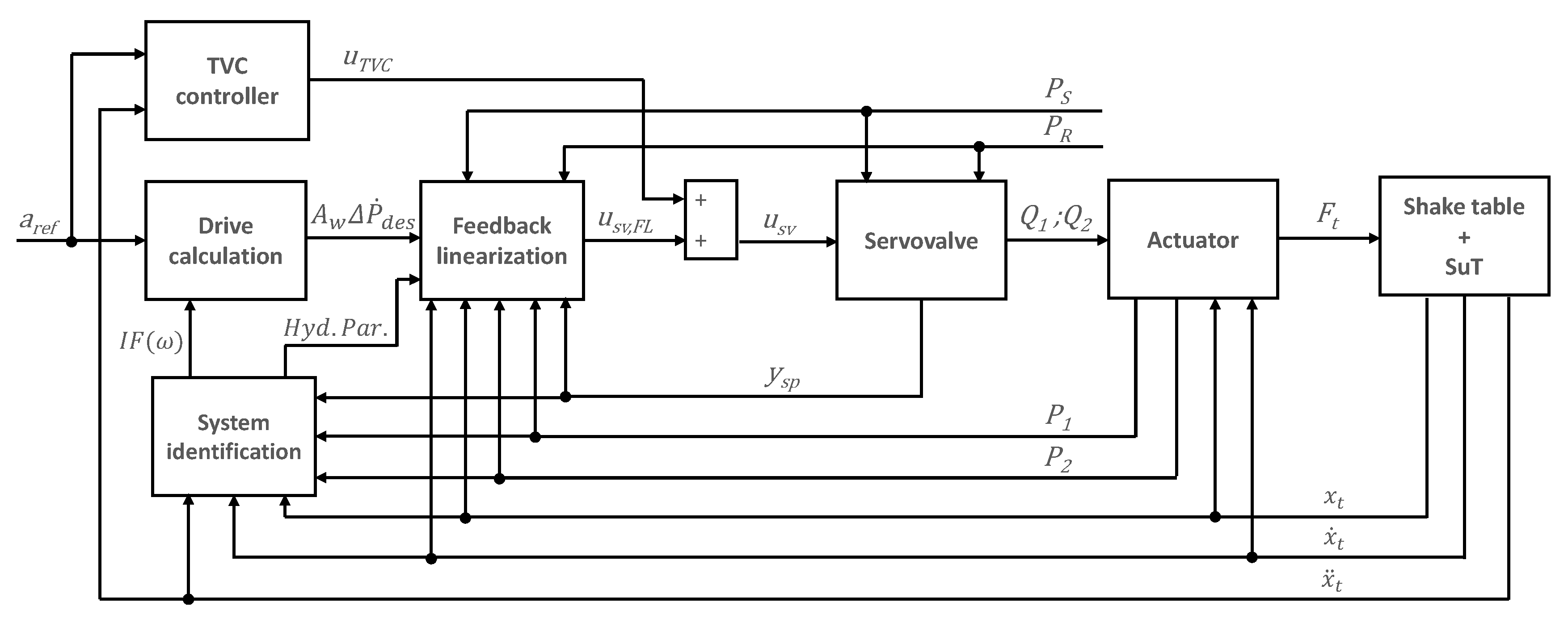
3. Description of the Proposed Control Methodology

The proposed control methodology comprises the following blocks:
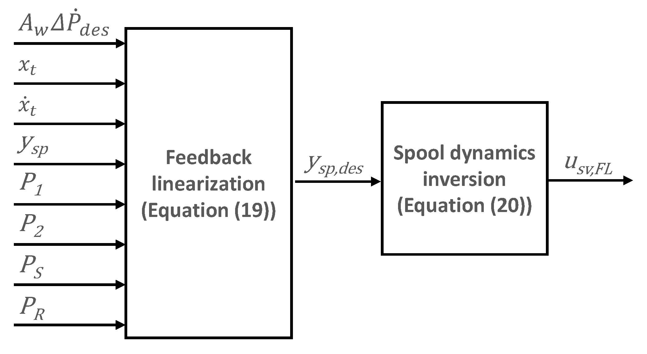
  • Feedback linearization. The purpose of this block is to cancel out, at least approximately, the non-linearities inherent to the servovalve-actuator system, leading to a control scheme where the time derivative of the pressure force exerted on the servoactuator’s piston rod can be directly imposed.
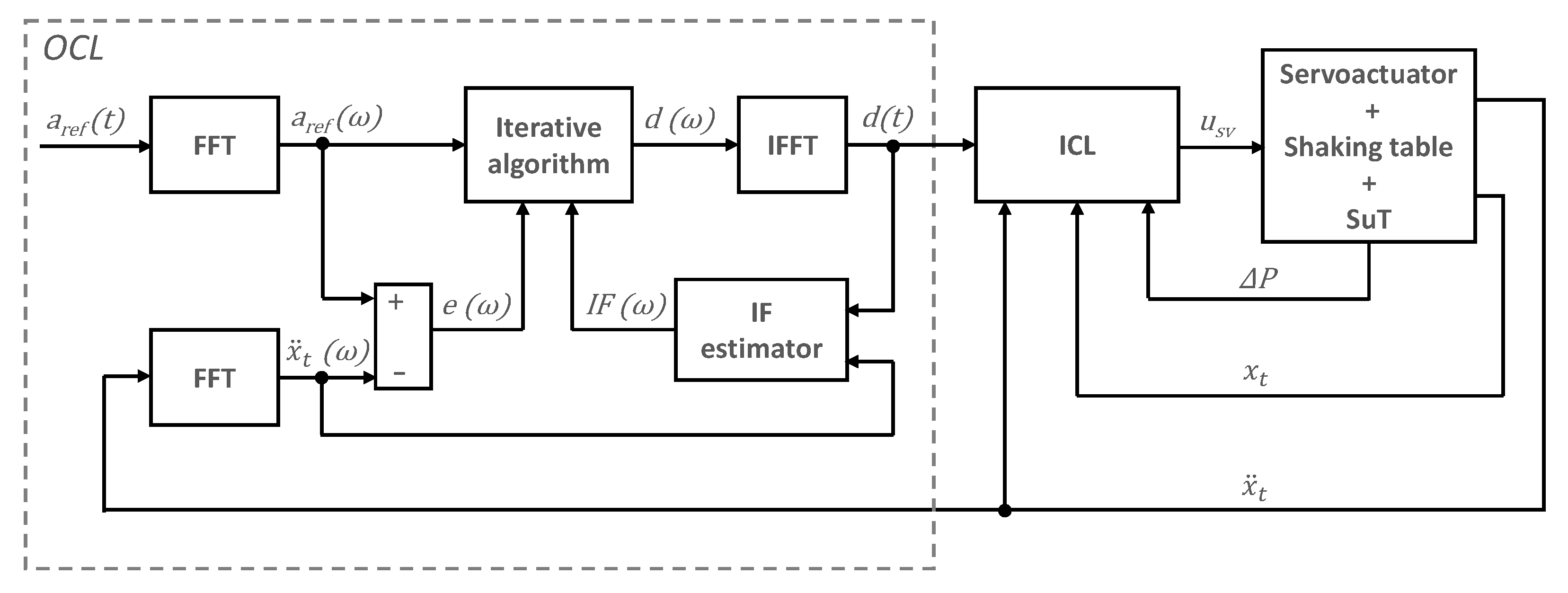
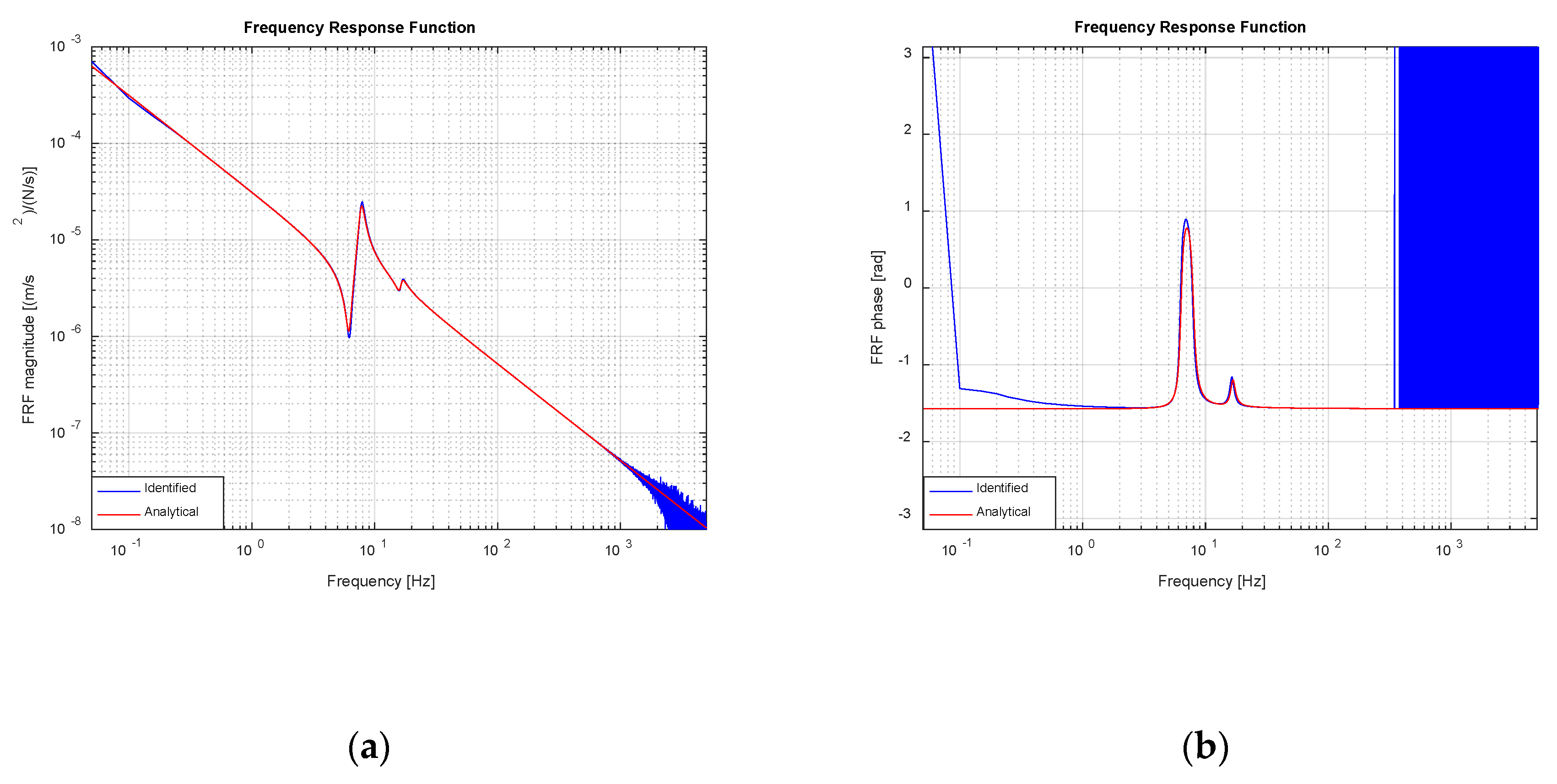
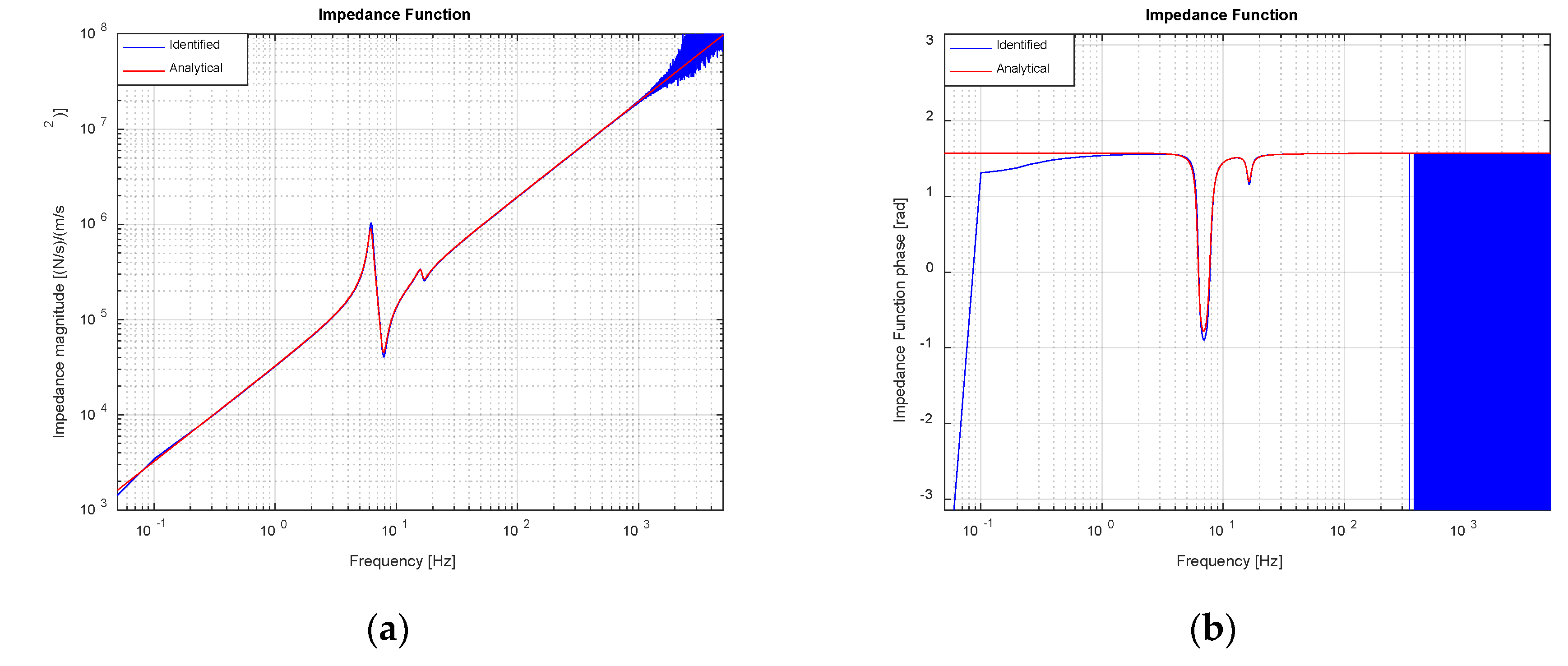
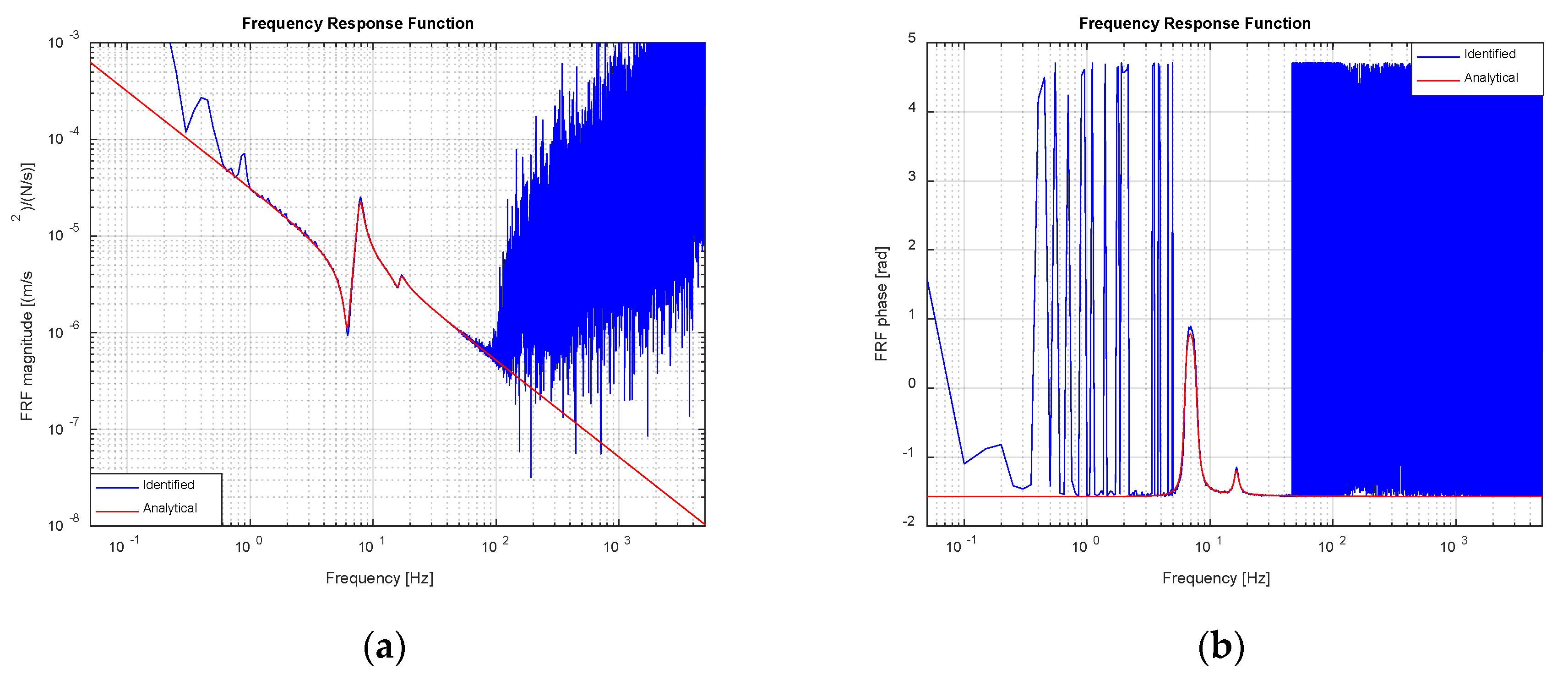
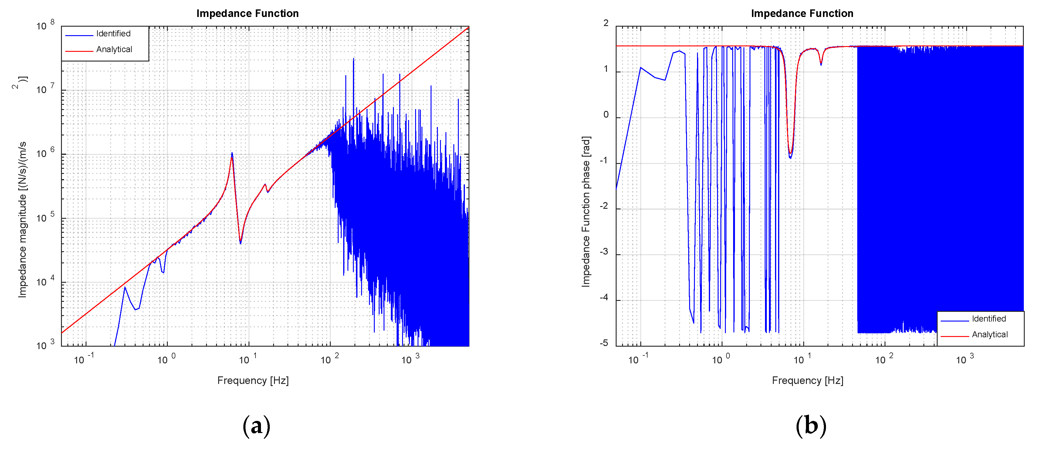
  • System identification. This module operates when the system is in identification mode, prior to the test itself. It is in charge of: (i) estimating and inverting the Accelerance Function (AF), which later is transformed into a more suitable IF representing the inverse model of the shake table-SuT system, and (ii) obtaining approximations for the values of the hydraulic parameters required by the feedback linearization scheme. It can also be implemented to operate, on a signal block basis, refining identification of IF and system parameters between one signal block and the following, as the test proceeds.
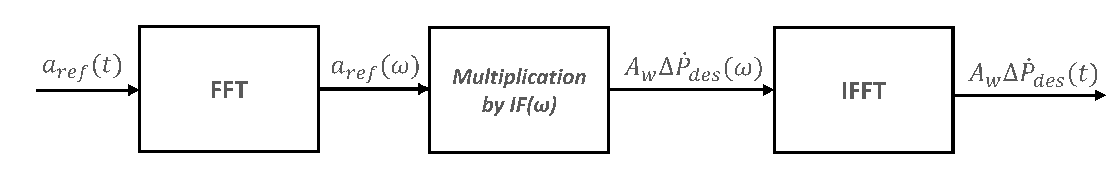
  • Drive calculation. This algorithm operates when the system is in test mode, on a signal block basis. It calculates the necessary pressure force time derivative to be applied on servoactuator’s rod by multiplying the IF from the system identification module by the desired acceleration output, in frequency domain, and transforming the result back into time domain.
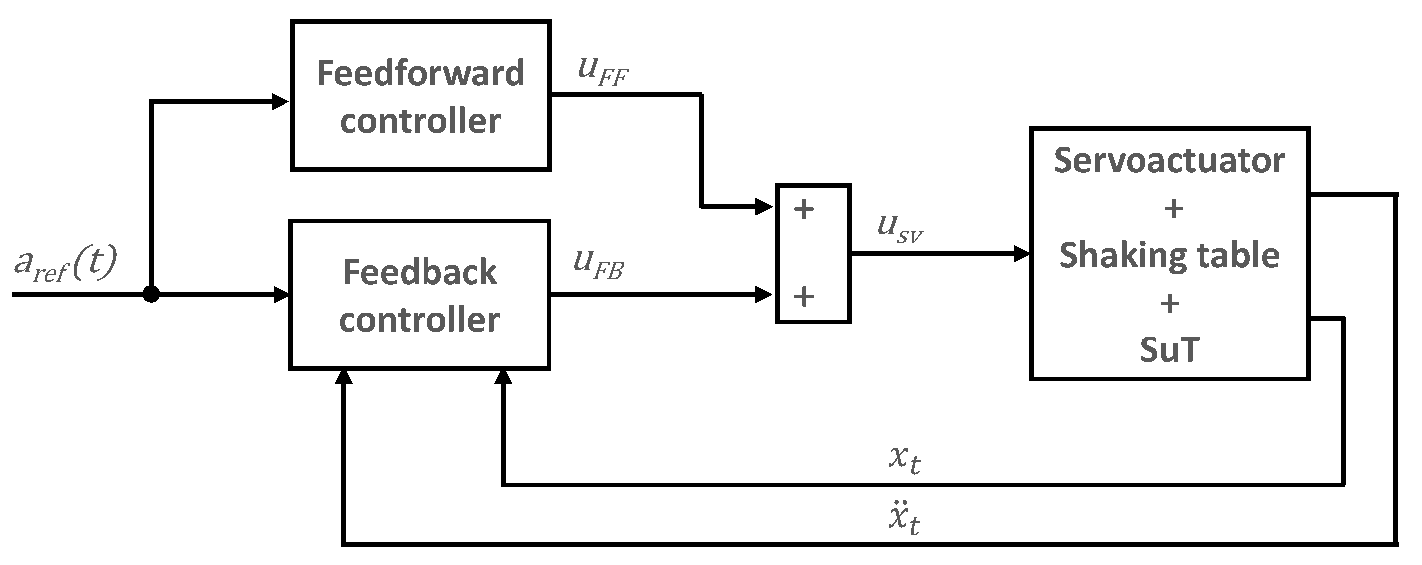
  • TVC controller. This feedback controller is necessary to compensate for the unavoidable imperfections present in the identified inverse model and to ensure overall system stability. It is implemented in parallel with the abovementioned architecture and accounts for errors in displacement, velocity and acceleration tracking in real-time.
Figure 5 shows a block diagram of the proposed control procedure, illustrating the interconnections between the previously enumerated modules. The proposed control methodology requires measuring the following variables: table (rod) displacement x t , rod acceleration x ¨ t , spool position y s p , pressure at actuator’s chambers P 1 and P 2 , pressure and return pressures P S and P R at the servovalve’s manifold and estimating the value of rod velocity, x ˙ t [24,25].

3.1. Feedback Linearization

Given a state-space representation of a multiple-input-multiple-output non-linear system: x ˙ = f ( x , u ) ;   y = g ( x ) , the aim of the feedback linearization scheme is to find a state transformation, z = z ( x ) and an input transformation, u = u ( x , v ) , such that the non-linear system is transformed into an equivalent linear system of the form z ˙ = A z + B v [26,27].
In the case under study, the non-linearities are present in servovalve flow-pressure (Equations (2) and (3)) and in chambers pressure time evolution expressions (Equations (4) and (5)). In this work, a direct approach has been employed to work out feedback linearization transformation.
By rearranging Equations (4) and (5), leaving the pressure derivatives on the left hand side, assuming β 1 = β 2 = β , and subtracting them, the time derivative of the pressure force acting on rod can be casted as:
( P ˙ 1 P ˙ 2 ) A w = β A w ( Q 1 v 01 + A w x p + Q 2 v 02 A w x p )   β A w 2 x ˙ p ( 1 v 01 + A w x p + 1 v 02 A w x p )   β A w C l 12 ( P 1 P 2 ) ( 1 v 01 + A w x p + 1 v 02 A w x p )   β A w ( C l 1 B ( P 1 P B 1 ) v 01 + A w x p C l 2 B ( P 2 P B 2 ) v 02 A w x p )
Now, for the case y s p 0 , if Equations (2) and (3) are substituted in Equation (10), the following expression is obtained:
( P ˙ 1 P ˙ 2 ) A w = y s p · F 1 + ( P 1 , P 2 , P S , P R ,   x p ) +   F 2 + ( x p ,   x ˙ p ) + F 3 + ( P 1 , P 2 , x p ) ,
where:
F 1 + ( P 1 , P 2 , P S , P R ,   x p ) = β A w C d K s v ( s g n ( P s P 1 ) 2 | P s P 1 | / ρ   v 01 + A w x p + s g n ( P 2 P R ) 2 | P 2 P R | / ρ v 02 A w x p ) ,
F 2 + ( x p ,   x ˙ p ) = β A w 2 x ˙ p ( 1 v 01 + A w x p + 1 v 02 A w x p ) ,
and
F 3 + ( P 1 , P 2 , x p ) = β A w [ C l 12 ( P 1 P 2 ) ( 1 v 01 + A w x p + 1 v 02 A w x p ) + ( C l 1 B ( P 1 P B 1 ) v 01 + A w x p C l 2 B ( P 2 P B 2 ) v 02 A w x p ) ] .
When y s p < 0 , Equation (3) is substituted in Equation (10) and the time derivative of pressure force results in:
( P ˙ 1 P ˙ 2 ) A w = y sp · F 1 ( P 1 , P 2 , P S , P R ,   x p ) +   F 2 ( x p ,   x ˙ p ) + F 3 ( P 1 , P 2 , x p ) ,
where:
F 1 ( P 1 , P 2 , P S , P R ,   x p ) = β A w C d K s v ( s g n ( P 1 P R ) 2 | P 1 P R | / ρ   v 01 + A w x p + s g n ( P S P 2 ) 2 | P S P 2 | / ρ v 02 A w x p ) ,
F 2 ( x p ,   x ˙ p ) = F 2 + ( x p ,   x ˙ p ) ,
and
F 3 ( P 1 , P 2 , x p ) = F 3 + ( P 1 , P 2 , x p ) .  
Let us now define a desired change in pressure force time derivative, A w Δ P ˙ d e s . Then, if the spool position y s p could be forced to instantaneously take the values defined by:
y s p = { A w Δ P ˙ d e s F 2 + ( x p ,   x ˙ p ) F 3 + ( P 1 , P 2 , x p ) F 1 + ( P 1 , P 2 , P S , P R ,   x p )   ;   y s p , p r e v 0 A w Δ P ˙ d e s F 2 ( x p ,   x ˙ p ) F 3 ( P 1 , P 2 , x p ) F 1 ( P 1 , P 2 , P S , P R ,   x p )   ;   y s p , p r e v < 0
( P ˙ 1 P ˙ 2 ) A w = A w Δ P ˙ d e s would hold, and an arbitrary time variation of pressure force could be imposed on the servoactuator. Above, y s p , p r e v denotes the value of the spool position at the previous iteration of the real-time control system, in which feedback linearization scheme is implemented.
This is the core idea to the control procedure presented in this work: finding the required time derivative of pressure force on the actuator’s rod, so that the acceleration reference profile is fulfilled. Due to the feedback linearization transformation found (Equation (19)), this value of A w Δ P ˙ d e s will be effectively imposed on servoactuator’s rod.
In order to force the spool position to accurately track the value determined by Equation (19), a servovalve spool dynamics inversion algorithm must be implemented. Assuming that spool motion is governed by the first order system in Equation (1), the dynamics inversion can be expressed as:
C s p u s v , F L = τ s p y ˙ s p , d e s + y s p , d e s ,
in which u s v , F L is the voltage output of the spool dynamics inversion algorithm and y s p , d e s is the desired spool position obtained from Equation (19). The calculation of the required voltage input to the servovalve therefore implies calculating the time derivative of y s p , d e s . For that purpose, a fourth order backward differentiation scheme has been utilized here [28]:
y ˙ n = 3 y n 4 16 y n 3 + 36 y n 2 48 y n 1 + 25 y n 12 Δ t
where n denotes the actual time step, y n the function evaluated at that time step and Δ t the time step which equals 1   ×   10 4 s (see Table 1). Figure 6 illustrates the block diagram of the described feedback linearization scheme.

3.2. System Identification

As mentioned before, the aim of the system identification module is twofold: (i) to work out an estimate of system’s IF and (ii) to identify hydraulic system parameters which are required to carry out feedback linearization. These procedures are dealt with in next two subsubsections.

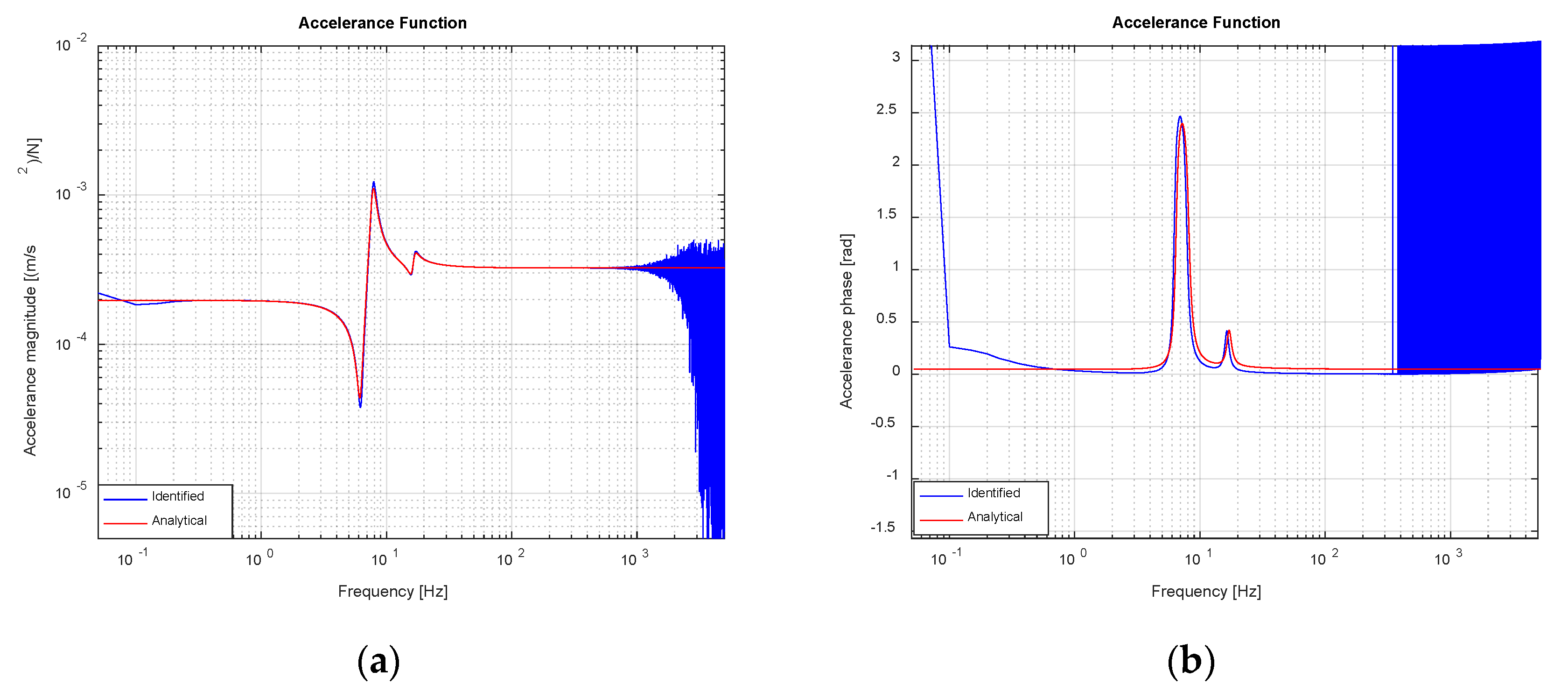
3.2.1. Impedance Function Identification Procedure

The first step taken in finding a suitable approximation of the IF of the system has been to work out an estimate of its AF to later derive an appropriate IF. Two scenarios for IF identification are considered in what follows: (i) a noise-free environment and (ii) a more realistic situation in which noise contaminates servovalve voltage input and force and acceleration measurements. The former is presented for theoretical validation purposes, while the latter constitutes a robustness check of the IF identification procedure necessary to correctly assess the potential of the proposed methodology.
The followed procedure has been essentially the same for both cases and consists in feeding the servovalve with several (voltage) blocks of random stimuli and recording simultaneously the force on the table and the acceleration at the control point. These constitute, respectively, the input and the output of the shake table-SuT system (see Figure 5). Later on, the AF has been estimated making use of classical FRF estimation algorithms [29]. In the noise-free environment the H 1 estimator has been employed. With this approach the AF is expressed as A F ( ω ) = G A F ( ω ) / G F F ( ω ) , where G A F ( ω ) is the cross-spectrum between force and acceleration and G F F ( ω ) is force autospectrum. For the noise-contaminated scenario, the H v estimator, which minimizes the effect of the noise at both the input and the output of the system, has been employed.
The input to the servovalve has been selected to be a gaussian random waveform with a duration of 20 s, a flat frequency content between 0.1 Hz and 100 Hz and a maximum amplitude of 20 mV. This signal has been windowed with a unit square signal with a duty cycle of 50%. In this way, excitation is only effective during the first half of the block, allowing for system response (acceleration) to attenuate towards the end of the block, therefore minimizing leakage errors. Figure 7 shows signals obtained in one iteration of the identification stage in time and frequency domains.
The AF approximation has been computed by linearly averaging the results obtained with sixteen input-output blocks. Figure 8 shows the achieved estimate for AF and its theoretical shape calculated analytically by transforming into frequency domain Equation (9) and performing the appropriate manipulations.
As it was explained in Section 3.1, the feedback linearization scheme, in theory, allows for the imposition of an arbitrary time derivative of pressure force exerted on actuator’s rod. Consequently, the IF sought must relate table acceleration to the time derivative of pressure force. This frequency function can be easily obtained by differentiating in frequency domain, without resorting to perform numerical derivatives on the desired pressure force obtained in time domain. Figure 9 and Figure 10 show the FRF (acceleration over pressure force time derivative) and the IF (pressure force time derivative over acceleration) finally used by the drive calculation module, along with their theoretical value. The quality of the identified inverse model is quite acceptable within the complete frequency range of interest, except for the very low frequencies and in the neighborhood of the first modal frequency of the system under control, where small differences can be observed.
In order to correctly assess the potential of the proposed methodology in a more realistic scenario, in what follows, the outcomes of an IF identification procedure in which servovalve voltage, force and acceleration signals have been influenced by electrical noise is presented.
The noise in measurements has been simulated by adding gaussian noise to servovalve input voltage and force and acceleration signals. The peak magnitude of the noise has been set to u n , p e a k = 0.01 V (see Section 2), which is an attainable value, when good industrial practices for low distance voltage signals wiring and shielding are observed. Later, the value of the noise affecting the physical quantities has been calculated by multiplying the electrical noise by each sensor’s gain as explained in Section 2. Figure 11 and Figure 12 show, in the presence of noise, the same information as Figure 9 and Figure 10. Clearly, the quality of the estimates of FRF and IF decreases; nevertheless, identification error remains within reasonable limits and the obtained estimates are sufficiently good in the whole frequency range of interest. So as to better compare the FRF estimates, coherence functions associated to FRF identification, both in the noise-free and noise-contaminated cases are shown in Figure 13. The coherence function is defined as γ 2 = | G F A ( ω ) | 2 / [ G F F ( ω ) G A A ( ω ) ] and measures the degree of linear relationship between two signals. Even though coherence in the noise-contaminated case is evidently worse than its noise-free counterpart, its values remain quite close to unity in the frequency range of interest, consequently confirming the validity of the FRF and IF estimates in the presence of noise of a reasonable magnitude.

3.2.2. Hydraulic Parameters Identification Procedure

The implementation of the feedback linearization scheme implies knowing accurate estimates of hydraulic parameters. In order to identify the sought values, and taking advance of the collection of data available from IF identification stage, a linear state-space model of the servoactuator has been identified. The inputs to this state-space model are, on the one hand, the voltage input to the servovalve, u s v , and the force exerted on piston rod,   F p , by the shake table, on the other. The latter can be calculated by means of:
F p = m p x ¨ t ( P 1 P 2 ) A w + F f r , p ,
which would correspond to the reading of a load cell installed between rod tip and shake table.
The state variables of the model have been selected as the velocity of the piston rod, which, as mentioned before, is identical to table velocity, x ˙ t , the difference of pressures across chambers denoted by Δ P and the servovalve’s main spool position, y s p . It has been assumed that Bulk moduli of each compartment are identical and are denoted by β . As mentioned in Section 2, the leakage flows between chambers and from chambers to bearings have been neglected. Accounting for these assumptions and linearizing Equations (1)–(5) around the mid-stroke operating point of the hydraulic cylinder, leads to the following analytical form of the state equations of the servoactuator system:
{ x ¨ t Δ P ˙ y ˙ s p } = [ C p / m p A w / m p 0 2 A w β / v 0 0 2 C d K s v β P s / ρ / v 0 0 0 1 / τ s p ] { x ˙ t Δ P y s p } + [ 0 1 / m p 0 0 C s p / τ s p 0 ] { u s v F p }
By means of a least squares procedure, the components of the matrices in Equation (23) have been identified. This process implies approximating the values of the rod velocity x ˙ t and time derivatives of state variables Δ P and y s p (see Equation (21)).
Once the estimates of matrices components are available, it is possible to estimate directly the values of A w , β / v 0 , C d K s v 2 / ρ , τ s p and C s p used in the feedback linearization scheme and also the values of m p and C p . In this work, it has been considered that the initial volumes of actuators chambers are known, and therefore, β can be estimated from β / v 0 value.
A check of the robustness against noise of the hydraulic parameters estimation process has been performed in the same way as for the IF estimation case. Table 2 shows the nominal and identified values of the hydraulic parameters and the identification relative error both for the noise-free and noise-contaminated identification cases. Despite the fact that parameters estimation quality decreases when a noisy environment is considered, the obtained values still represent with reasonable accuracy system actual parameters.

3.3. Drive Calculation Module

The drive calculation module computes the desired pressure force time derivative to be injected to the feedback linearization module. Firstly, the reference acceleration profile is transformed into frequency domain by means of an FFT process. Then, the drive signal is calculated multiplying the identified IF by the transformed acceleration profile. Finally, the result is transformed back into time domain by means of an IFFT process. Figure 14 schematizes the described process.

3.4. Three Variable Controller

A feedback controller has been implemented, in parallel with the previously described architecture, with the aim to cope with the unavoidable errors occurring within AF and hydraulic parameters identification processes. TVC philosophy has been adopted so as to provide real-time simultaneous corrections to rod displacement, velocity and acceleration errors. The control law of the TVC is defined as follows:
u T V C = K d ( d r e f x p ) + K v ( v r e f x ˙ p ) + K a ( a r e f x ¨ p ) ,
where u T V C is the control voltage output by TVC, d r e f , v r e f , a r e f are respectively the displacement, velocity and acceleration reference waveforms and K d , K v and K a are the control gains for displacement, velocity and acceleration errors. As it can be noticed, the implementation of this controller requires calculating, by integration, the reference displacements and velocities from the given reference acceleration.

4. Numerical Simulations Results and Control Methods Comparison

In this section, the numerical results obtained with the model described in Section 2 are presented. Section 4.1. shows and discusses simulation results for the new proposed control method in scenarios with and without noise present in measurements from sensors. Section 4.2 compares the performance of the suggested control procedure to that of the classical iterative control approach illustrating the main differences.

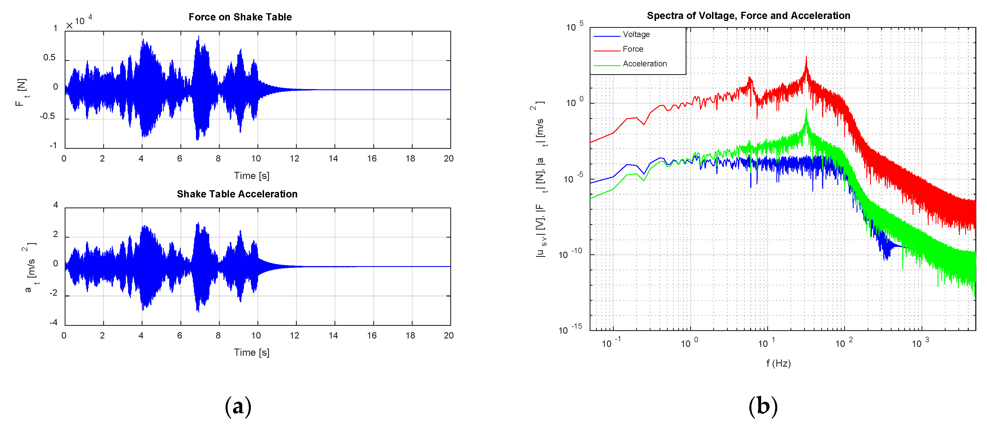
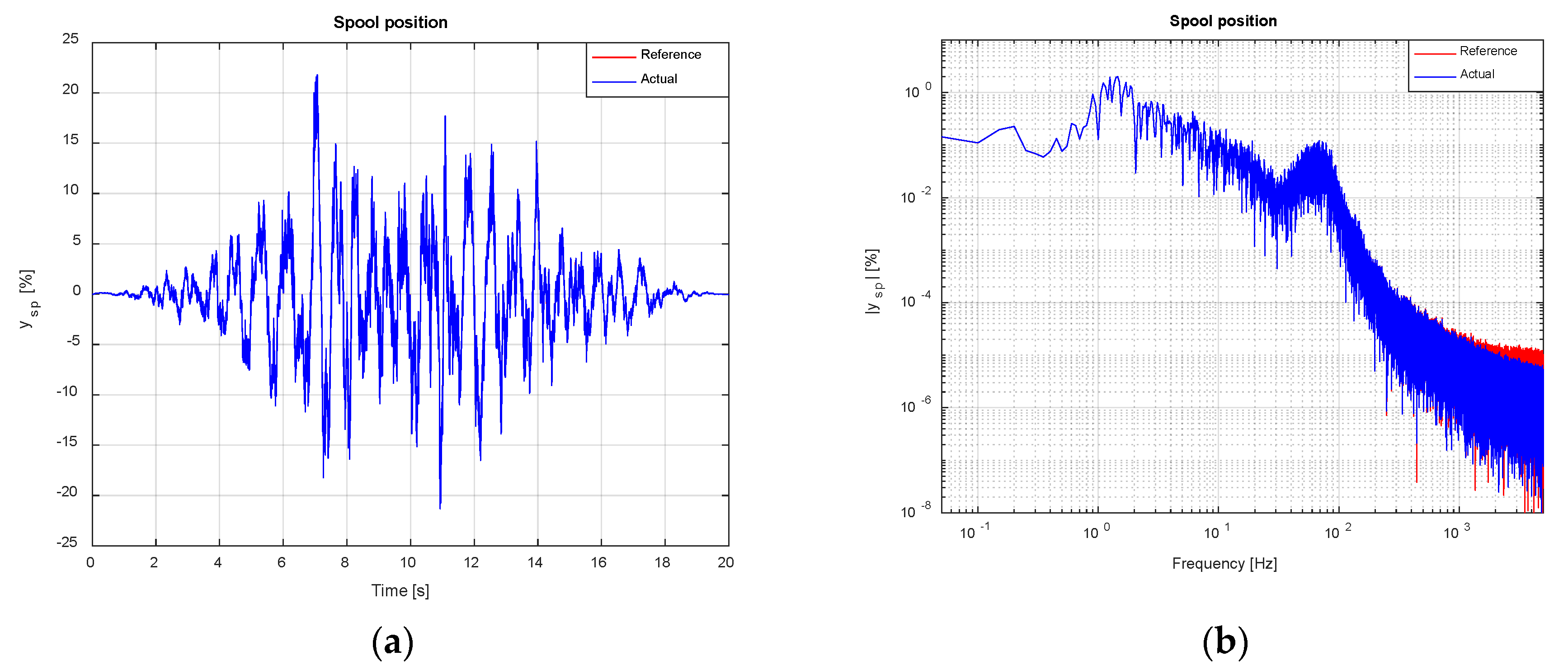
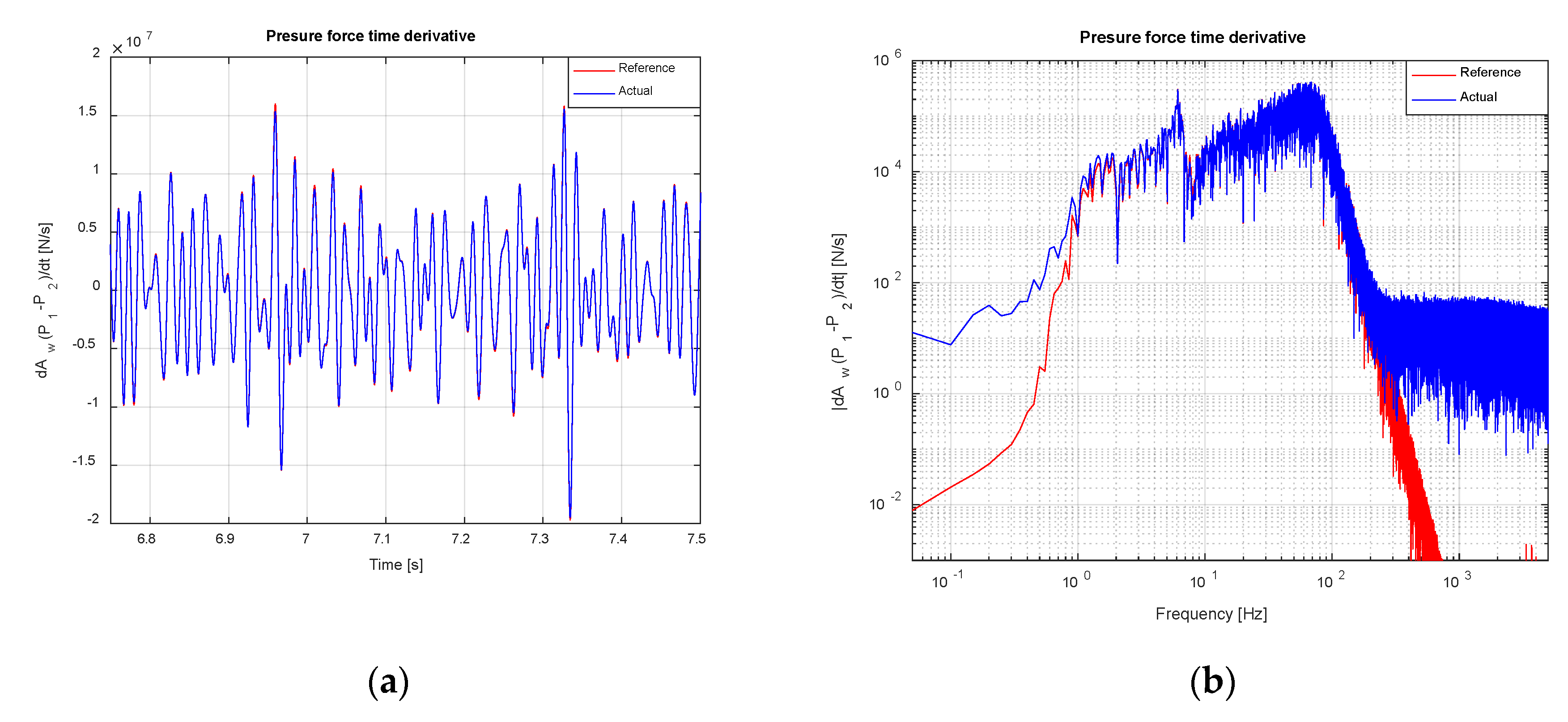
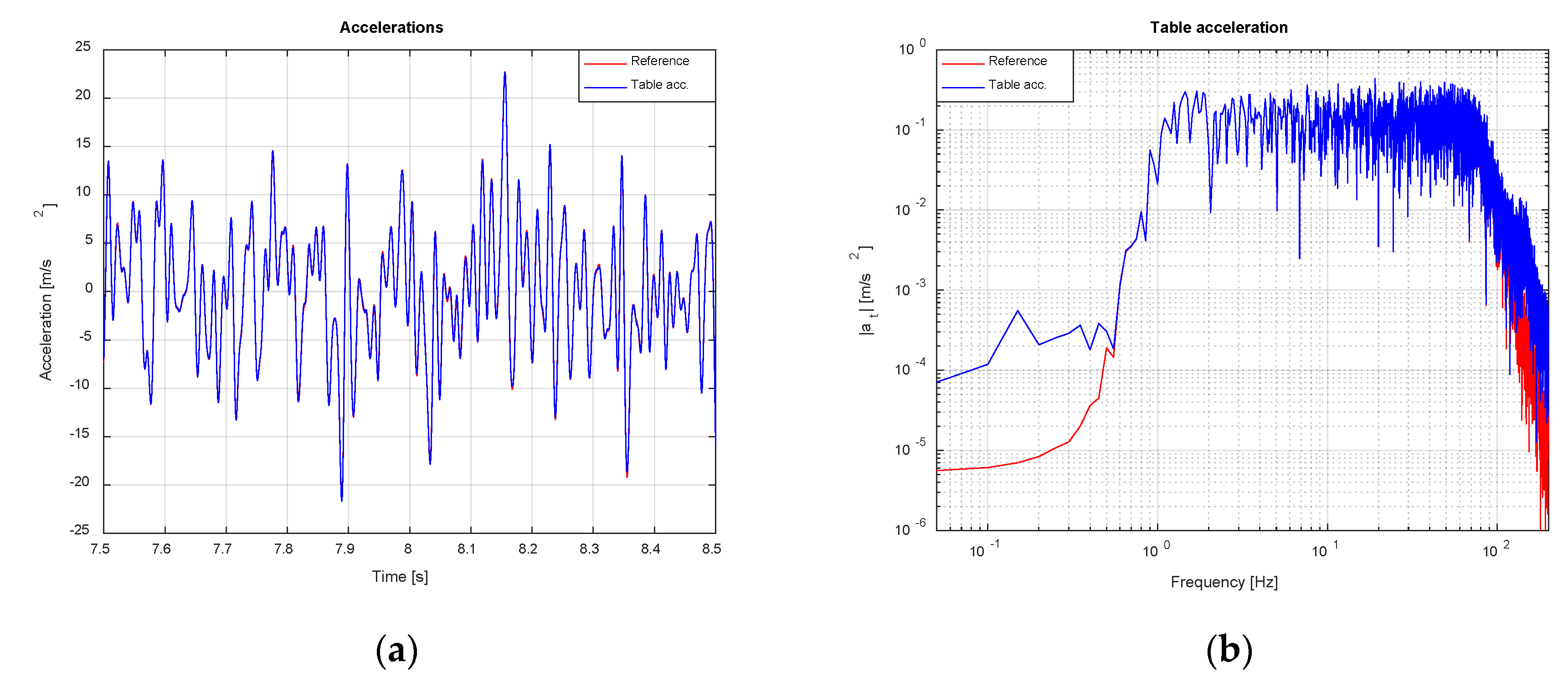
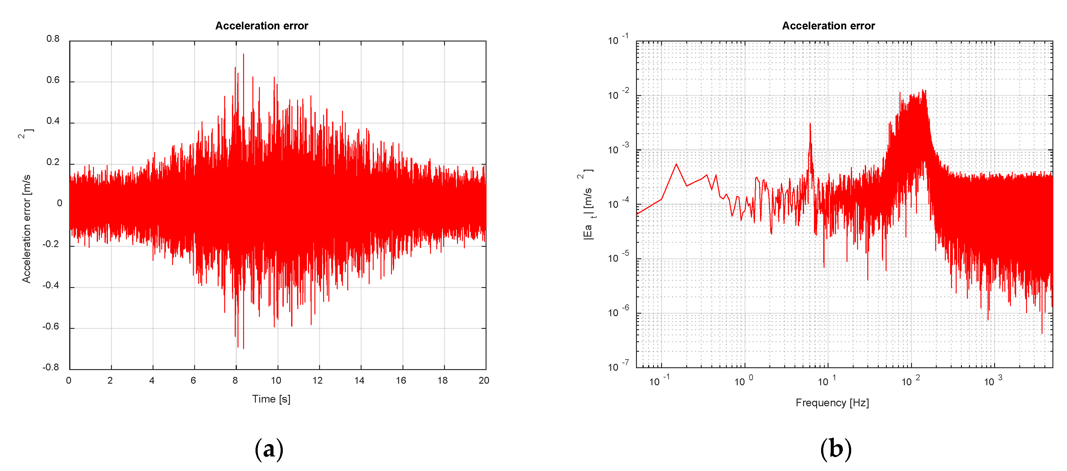
4.1. Numerical Simulations Results

The chosen acceleration reference in all the presented cases is a random gaussian waveform with a duration of 20 s and a flat frequency content between 1 Hz and 80 Hz (see Figure 17). A Hanning window has been applied to the reference profile to ensure null values at the block ends. The approximate peak displacement, velocity and acceleration values are 30 mm, 0.4 m/s and 25 m/s2. A fixed step solver and a time step of 1   ×   10 4 s has been used for all the simulations in this section.
A first set of simulations has been carried out with the TVC feature disabled in a noise-free environment. As explained in Section 3.1, the feedback linearization module calculates an instantaneous spool position, which is attempted to be imposed on servovalve’s main stage by means of a spool dynamics inversion algorithm (see Equation (20)). Figure 15 shows the reference and achieved servovalve spool position, both in time and frequency domain. It can be concluded that the tracking achieved by the dynamic inversion algorithm is accurate within the whole frequency range of interest.
The time derivative of pressure force on actuator’s rod, synthesized by the drive calculation module explained in Section 3.3, and the actual one effectively imposed on servoactuator owing to the feedback linearization process, are shown in Figure 16. Figure 16a has been zoomed around the area where maximum error takes place. Tracking is acceptable in the entire frequency range of interest with larger errors at low frequencies and around the first modal frequency of the table-SuT system, due to the poorer IF estimate obtained at those frequency values (see Figure 10).
Figure 17 shows the target acceleration together with the one attained in numerical simulations. A tracking error of approximately 0.55 m/s2 rms has been achieved. As in the previous case, and due to the same reasons stated there, reference acceleration tracking is reasonably satisfactory, except for the low frequencies and at the neighborhood of the first modal frequency of the system. Acceleration tracking error is shown in more detail in Figure 18. Despite the fact that tracking can be deemed acceptable, accumulation of errors within the low frequency region lead to increased velocity errors and displacement drifts which may hinder successful test execution due to limited servovalve flow rate capacity and actuator stroke. Therefore, it seems mandatory to enhance the control architecture with a parallel controller able to keep, simultaneously, all kinematic variables tracking errors within reasonable limits.
A second round of simulations has been carried out with the TVC feature enabled in a noise-free environment. Figure 19, Figure 20 and Figure 21 show the same information as that offered in Figure 16, Figure 17 and Figure 18. The employed values of TVC control gains have been K d   = 1, K v   = 0.5 and K a = 0.25 . Figures below show a drastic decrease in acceleration tracking error of from 0.55 m/s2 rms in the previous case to 0.087 m/s2. This reduction especially marked in the low frequency range, down to 0.6 Hz, confirming the effectiveness of the TVC feedback controller.
A third set of simulations has been carried out to assess the suggested control method in a scenario where noise is present in sensors measurements. The electrical noise has been modelled as a gaussian waveform with a peak value of 10 mV according to considerations made in Section 3.2.1. Sources of noise of this magnitude have been added to all the transducers present in the model (displacement, acceleration, chamber pressures and spool position) and to servovalve input voltage. Noise in voltage has been multiplied by the appropriate gains to translate it into the physical quantities affecting the model (see Section 2). The drive estimate has been synthesized making use of the IF obtained in a noisy environment (see Section 3.2.1) and the hydraulic parameters utilized by feedback linearization scheme have been those estimated in presence of noise. The TVC feature has been enabled and the control gains used have been the same as in the previous case, that is, K d   = 1, K v   = 0.5 and K a   =   0.25 .
Figure 22, Figure 23 and Figure 24 show the same information as that in Figure 19, Figure 20 and Figure 21. An overall tracking error of 0.403 m/s2 rms has been achieved. Tracking error has increased in the whole frequency range and specially around the higher frequency limit of the reference profile. The effect of noise is obviously more accused at lower target acceleration values due to the reduced signal to noise ratio at those sections. Nevertheless, despite the fact that electrical noise clearly affects negatively tracking quality, performance is still reasonably good and the stability of the system is maintained, therefore confirming the robustness of the proposed method when electrical noise of a reasonable magnitude contaminates sensors measurements.
Finally, a fourth round of simulations has been conducted to explore the trend of system behavior in a noisy environment, when the values of the control gains of the TVC are increased while keeping the rest of the parameters unaltered. The values of the control gains employed have been K d   = 3, K v   = 2 and K a = 1 . Figure 25 and Figure 26 show, respectively, acceleration and acceleration error both in time and frequency domain. With the employed control parameters, the influence of the noise in the system is remarkably reduced yielding similar results as in the second set of simulations. In particular, a tracking error of 0.1154 m/s2 rms has been attained.

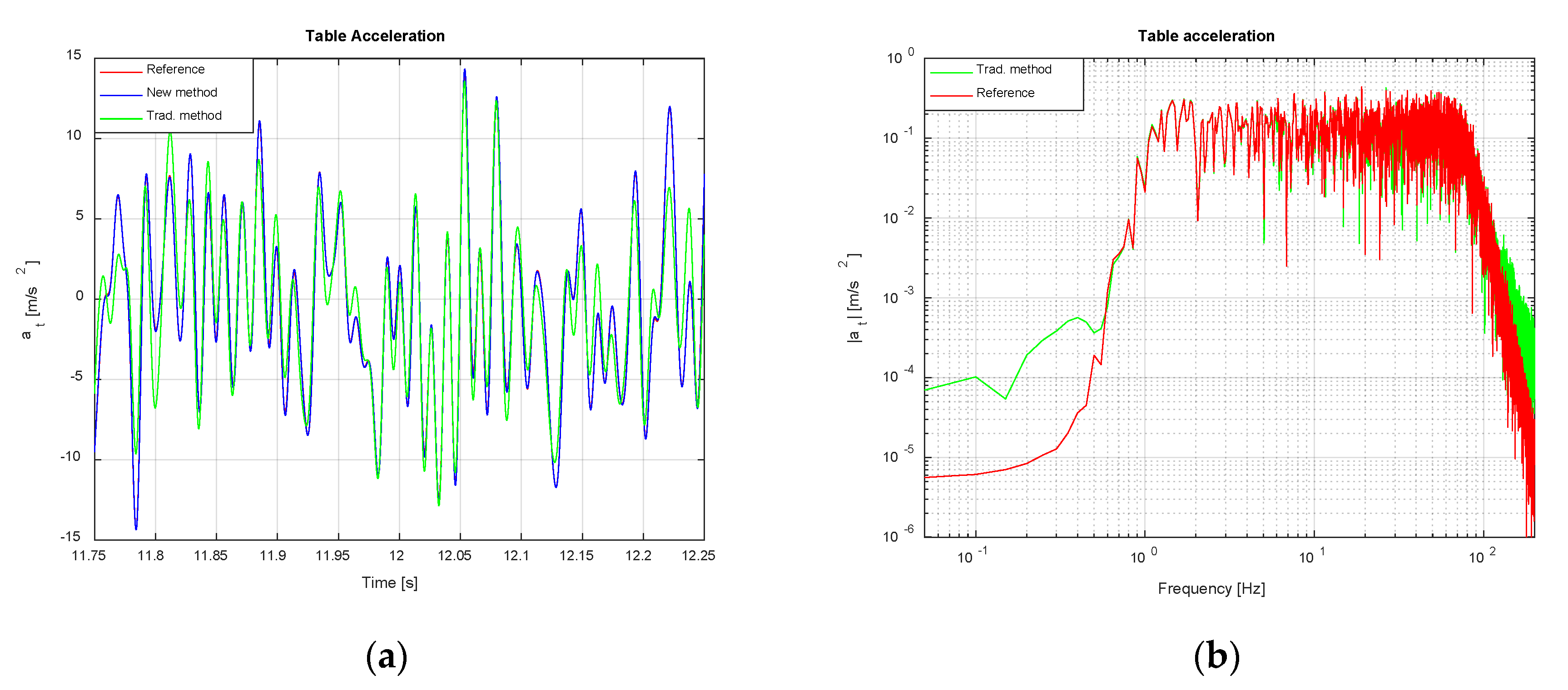
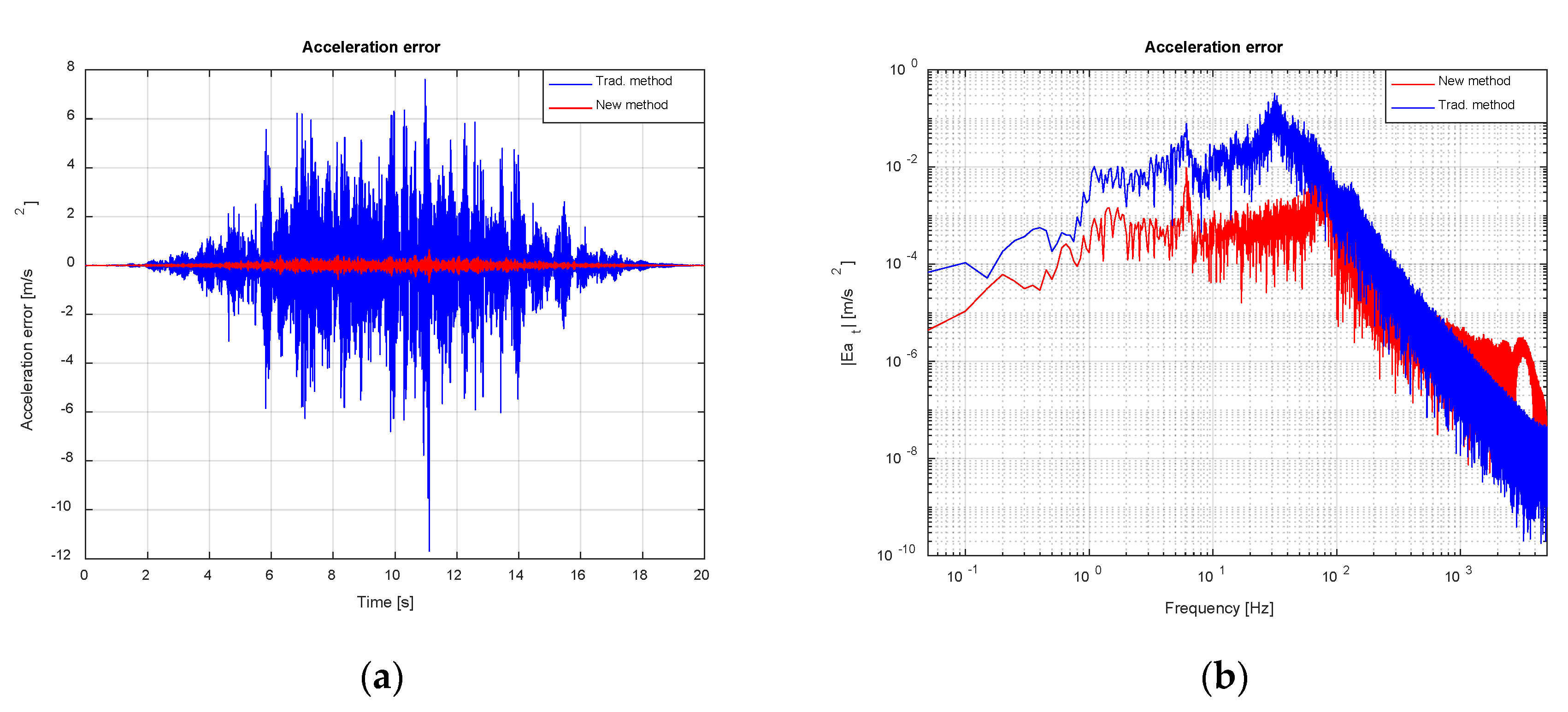
4.2. Comparison between Control Methods

In this subsection, a comparison between the classical iterative control approach, which constitutes the industry standard for shake table testing, and the new proposed method is presented. A generic iterative scheme (see Figure 2), in a noise-free scenario, has been employed to obtain qualitative results representative of the classical method performance. First off, the FRF of the system has been identified making use of the H 1 estimator, according to traditional approach (acceleration over voltage). Then, it has been inverted to obtain the IF (voltage over acceleration). An estimate of the initial drive to be fed to the system has been calculated by means of: d 0 ( ω ) = I F ( ω ) a r e f ( ω ) , where d 0 ( ω ) is the initial drive in frequency domain. The result has been transformed into time domain by means of an IFFT and has been injected into the servovalve. After the initial iteration, the drive signal would be updated in successive runs by an iterative scheme of the form: d n + 1 ( ω ) =   d n ( ω ) + k I F ( ω ) [ x ¨ t n ( ω ) a r e f ( ω ) ] , formulated in frequency domain, where n denotes iteration number and k is the correction gain. However, only the acceleration results obtained at the first iteration have been considered, with the aim of evaluating the control methods in comparable operation conditions. In these simulations, the TVC feature in the new control procedure has been enabled and the values of control gains used have been: K d   = 1, K v   = 0.5 and K a = 0.25 .
Figure 27 and Figure 28 show acceleration response and tracking error for both methods. The first iteration of classical approach reaches a tracking error of 1.484 m/s2 rms as opposed to the 0.087 m/s2 rms featured by the new implementation. The proposed method shows much better behavior than the first iteration of the classical approach over the complete frequency range. Nevertheless, this difference in performances is likely to decrease if a certain number of control iterations were carried out. According to Figure 28a, the error of the classical approach increases with the magnitude of the target acceleration. This tracking error rise is caused by the fact that this method relies on a linearization of a non-linear system around an operating point, which may no longer be valid when the target acceleration profile implies reaching large values of forces and displacements. In opposition, the new suggested procedure performs well even at high accelerations, in part, due to the fact that the implemented feedback linearization scheme excludes the non-linearities associated to hydraulic system from the control loop.

5. Conclusions

This paper presents a novel mixed time-frequency acceleration control method for shake table systems. The suggested procedure includes identifying an FRF-IF pair which relates table acceleration to the time derivative of the pressure force acting on servoactuator’s piston rod prior to the test. This approach allows for the calculation of a time variation of pressure force waveform which can be directly imposed by means of a feedback linearization scheme, which approximately cancels out non-linearities associated hydraulic actuation system leaving only those related to SuT present in the control loop. Modeling errors, feedback linearization imperfections and external perturbations are dealt with by a TVC implemented in parallel with the previously outlined architecture. Consequently, this method includes features belonging to time and frequency domain methods usually employed in shake table control systems.
The potential effectiveness of the methodology was assessed by means of numerical simulations carried over a model of the shake table loaded with a two stories shear building. Four groups of numerical simulations were performed:
  • without the parallel TVC feature enabled in an electrical noise free environment;
  • with the parallel TVC feature enabled in a noise-free environment;
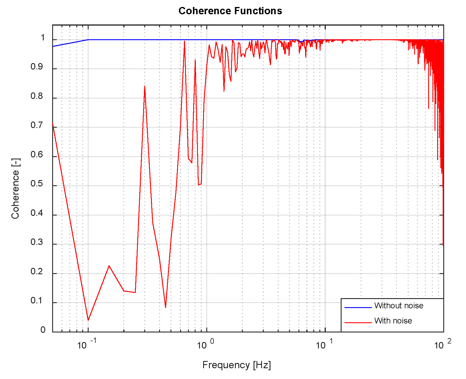
  • with the parallel TVC feature enabled in an electrical noise contaminated environment;
  • with the same conditions as in 3. but with a better tuning of TVC parameters.
Results corresponding to the first group show quite acceptable acceleration tracking; however, errors at low frequencies may lead to undesired table drifts. When the TVC feature is enabled and electrical noise is not considered (group 2), tracking errors are drastically reduced, leading to almost-perfect acceleration tracking with a low control burden placed on the TVC controller. Noise affects negatively the performance in the whole frequency range, as it was demonstrated by the third group of simulations; however, tracking error remains within acceptable limits and the stability of the system is preserved, thus confirming the robustness of the proposed control procedure when electrical noise of a reasonable magnitude contaminates sensors measurements. Finally, the fourth group of simulations demonstrates that, by a proper tuning of the TVC control parameters, almost-perfect tracking is possible even in the presence of noise. The performance of the new proposed method is better than that of the classical iterative approaches when these operate on a single iteration basis.
The presented method thus appears quite promising for its implementation in real systems and features the following advantages over traditional iterative methods: (i) no iterations are required in test execution stage, (ii) non-linearities associated to hydraulic actuation are excluded from the control loop, improving tracking characteristics and (iii) the method is less sensitive to uncertainties in IF identification than the traditional control approaches due to the parallel TVC feature.
The proposed methodology requires, however, measuring or estimating rod displacement, velocity and acceleration, pressures at both actuator’s chambers, pressures at supply and return ports of actuator manifolds and position of servovalve’s main stage spool position. Therefore, its implementation implies increased instrumentation needs with respect to that used in traditional control methods.
Current works are focused on the implementation of the proposed architecture in an actual shake table system, paying special attention to the following points:
  • Non-linearities present in the purely mechanical system.
  • Rigorous studies on the uncertainty in IF and hydraulic parameters estimation and on the effect of noise present in sensors measurements.
  • Development of differentiation schemes robust against noise in signals.
  • Assessment of the effects of the delay due to control loop and sensors and their effect on feedback linearization scheme.

Author Contributions

Conceptualization, J.R.S., J.H.G.-P. and I.M.D.; methodology, J.R.S.; software, J.R.S.; validation, J.R.S.; formal analysis, J.R.S.; investigation, J.R.S. and I.M.D.; resources, J.R.S.; data curation, J.R.S.; writing—original draft preparation, J.R.S.; writing—review and editing, J.R.S., J.H.G.-P. and I.M.D.; visualization, J.R.S.; supervision, J.H.G.-P. and I.M.D.; project administration, J.H.G.-P. and I.M.D.; funding acquisition, J.H.G.-P. and I.M.D. All authors have read and agreed to the published version of the manuscript.

Funding

This research was funded by Spanish Ministry of Science, Innovation and Universities through the project SEED-SD (RTI2018-099639-B-I00).

Acknowledgments

The authors would like to express their gratitude to Vzero Engineering Solutions, S.L. for providing several pictures.

Conflicts of Interest

The authors declare no conflict of interest.

References

  1. Williams, M.S.; Blakeborough, A. Laboratory testing of structures under dynamic loads: An introductory review. Philos. Trans. R. Soc. Lond. Ser. A 2001, 359, 1651–1669. [Google Scholar] [CrossRef]
  2. Füllekrug, U. Utilization of multi-axial shaking tables for the modal identification of structures. Philos. Trans. R. Soc. Lond. Ser. A 2001, 359, 1753–1770. [Google Scholar] [CrossRef]
  3. Severn, R. The development of shaking tables—A historical note. Earthq. Eng. Struct. Dyn. 2011, 40, 195–213. [Google Scholar] [CrossRef]
  4. Plummer, A.R. Control techniques for structural testing: A review. Proc. Inst. Mech. Eng. Part I J. Syst. Control Eng. 2007, 221, 139–169. [Google Scholar] [CrossRef]
  5. Bairrão, R.; Vaz, C.T. Shaking Table Testing of Civil Engineering Structures-The LNEC 3D Simulator Experience. In Proceedings of the 12th World Conference on Earthquake Engineering, Auckland, New Zealand, 30 January–4 February 2000. [Google Scholar]
  6. Yao, J.; Dietz, M.; Xiao, R.; Yu, H.; Wang, T.; Yue, D. An overview of control schemes for hydraulic shaking tables. J. Vib. Control 2014, 22, 2807–2823. [Google Scholar] [CrossRef]
  7. Hanh, D.L.; Ahn, K.K.; Kha, N.B.; Jo, W.K. Trajectory control of electro-hydraulic excavator using fuzzy self tuning algorithm with neural network. J. Mech. Sci. Technol. 2009, 23, 149–160. [Google Scholar] [CrossRef]
  8. Phillips, B.M.; Wierschem, N.E.; Spencer, B.F. Model based multi-metric control of uniaxial shake tables. Earthq. Eng. Struct. Dyn. 2014, 43, 681–699. [Google Scholar] [CrossRef]
  9. Najafi, A.; Spencer, B.F. Modified model-based control of shake tables for online acceleration tracking. Earthq. Eng. Struct. Dyn. 2020. [Google Scholar] [CrossRef]
  10. Plummer, A. Model-based motion control for multi-axis servohydraulic shaking tables. Control Eng. Pract. 2016, 53, 109–122. [Google Scholar] [CrossRef] [Green Version]
  11. Shen, G.; Zheng, S.T.; Ye, Z.M.; Yang, Z.D.; Zhao, Y.; Han, J.W. Tracking control of an electro-hydraulic shaking table system using a combined feedforward inverse model and adaptive inverse control for real-time testing. Proc. Inst. Mech. Eng. Part I J. Syst. Control Eng. 2011, 225, 647–666. [Google Scholar] [CrossRef]
  12. Nakata, N. Acceleration trajectory tracking control for earthquake simulators. Eng. Struct. 2014, 32, 2229–2236. [Google Scholar] [CrossRef]
  13. Seki, K.; Iwasaki, M.; Kawafuku, M.; Hirai, H.; Yasuda, K. Improvement of control performance in shaking-tables by feedback compensation for reaction force. In Proceedings of the 34th Annual Conference of the IEEE Industrial Electronics Society, Orlando, FL, USA, 10–13 November 2008; IEEE: New York, NY, USA, 2008; pp. 2551–2556. [Google Scholar] [CrossRef]
  14. Yao, J.; Di, D.T.; Jiang, G.L.; Gao, S. Acceleration amplitude-phase regulation for electro-hydraulic servo shaking table based on LMS adaptive filtering algorithm. Int. J. Control 2012, 85, 1581–1592. [Google Scholar] [CrossRef]
  15. Yao, J.; Hu, S.H.; Fu, W.; Han, J.W. Harmonic cancellation for electro-hydraulic servo shaking table based on LMS adaptive algorithm. J. Vib. Control 2011, 17, 1862–1868. [Google Scholar] [CrossRef]
  16. Nowak, R.F.; Kusner, D.A.; Larson, R.L.; Thoen, B.K. Utilizing modern digital signal processing for improvement of large scale shaking table performance. In Proceedings of the 12th World Conference on Earthquake Engineering, Auckland, New Zealand, 30 January–4 February 2000; pp. 2035–2042. [Google Scholar]
  17. Tagawa, Y.; Kajiwara, K. Controller development for the E-Defense shaking table. Proc. Inst. Mech. Eng. Part I J. Syst. Control Eng. 2007, 221, 171–181. [Google Scholar] [CrossRef]
  18. Stoten, D.P.; Gómez, E.G. Adaptive control of shaking tables using the minimal control synthesis algorithm. Philos. Trans. R. Soc. Lond. Ser. A 2001, 359, 1697–1723. [Google Scholar] [CrossRef]
  19. Stoten, D.P.; Shimizu, N. The feedforward minimal control synthesis algorithm and its application to the control of shaking-tables. Proc. Inst. Mech. Eng. Part I J. Syst. Control Eng. 2007, 221, 423–444. [Google Scholar] [CrossRef]
  20. De Cuyper, J.; Coppens, D.; Liefooghe, C.; Debille, J. Advanced system identification methods for improved service load simulation on multi-axial test rigs. Eur. J. Mech. Environ. Eng. 1999, 44, 27–39. [Google Scholar]
  21. Zhao, J.; Catharine, C.S.; Posbergh, T. Nonlinear system modeling and velocity feedback compensation for effective force testing. J. Eng. Mech. 2005, 131, 244–253. [Google Scholar] [CrossRef]
  22. Merrit, H.E. Hydraulic Control. Systems, 1st ed.; John Wiley & Sons: New York, NY, USA, 1991; pp. 76–100. [Google Scholar]
  23. Servovalves with Integrated Electronics D791 and D792 Series. Available online: www.moog.com/content/dam/moog/literature/ICD/Moog-Valves-D791_D792-Catalog-en.pdf (accessed on 24 September 2020).
  24. Stoten, D.P. Fusion of kinetic data using composite filters. Proc. Inst. Mech. Eng. Part. I J. Syst. Control. Eng. 2001, 215, 483–497. [Google Scholar] [CrossRef]
  25. Plummer, A.R. Optimal complementary filters and their application in motion measurement. Proc. Inst. Mech. Eng. Part. I J. Syst. Control. Eng. 2006, 6, 489–507. [Google Scholar] [CrossRef]
  26. Kwatny, H.G.; Blankenship, G.L. Nonlinear Control and Analytical Mechanics: A Computational Approach, 1st ed.; Birkenhäuser: Boston, MA, USA, 2000; pp. 185–201. [Google Scholar]
  27. Slotine, J.E.; Li, W. Applied Nonlinear Control., 1st ed.; Prentice-Hall, Inc.: Englewood Cliffs, NJ, USA, 1991; pp. 207–265. [Google Scholar]
  28. Press, W.H.; Teukolsky, S.A.; Vetterling, W.T.; Flannery, B.P. Numerical Recipes in Fortran. In The Art of Scientific Computing, 2nd ed.; Cambridge University Press: New York, NY, USA, 1992; pp. 180–184. [Google Scholar]
  29. Leclere, Q.; Roozen, B.; Sandier, C. On the use of the Hs estimator for the experimental assessment of transmissibility matrices. Mech. Syst. Signal. Process. 2014, 43, 237–245. [Google Scholar] [CrossRef] [Green Version]
Figure 1. Generic time domain control architecture for shake table.
Vibration 03 00027 g001
Figure 2. Generic frequency domain control architecture for shake table.
Vibration 03 00027 g002
Figure 3. Shake table system. Courtesy of Vzero Engineering Solutions, SL.
Vibration 03 00027 g003
Figure 4. Scheme of the shake table system modeled elements.
Vibration 03 00027 g004
Figure 5. Control architecture block diagram.
Vibration 03 00027 g005
Figure 6. Feedback linearization scheme.
Vibration 03 00027 g006
Figure 7. Identification signals (one block): (a) Force on table and table acceleration in time domain; (b) Servovalve voltage, Force on table and table acceleration in frequency domain.
Vibration 03 00027 g007
Figure 8. Identified and analytical AF (noise-free scenario): (a) Magnitude; (b) Phase.
Vibration 03 00027 g008
Figure 9. Identified and analytical FRF (noise-free scenario): (a) Magnitude; (b) Phase.
Vibration 03 00027 g009
Figure 10. Identified and analytical IF (noise-free scenario): (a) Magnitude; (b) Phase.
Vibration 03 00027 g010
Figure 11. Identified and analytical FRF (noise-contaminated scenario): (a) Magnitude; (b) Phase.
Vibration 03 00027 g011
Figure 12. Identified and analytical IF (noise-contaminated scenario): (a) Magnitude; (b) Phase.
Vibration 03 00027 g012
Figure 13. Coherence functions comparison.
Vibration 03 00027 g013
Figure 14. Drive calculation process.
Vibration 03 00027 g014
Figure 15. Spool position tracking (noise-free scenario). TVC disabled: (a) Time domain; (b) Frequency domain.
Vibration 03 00027 g015
Figure 16. Pressure force time derivative tracking (noise-free scenario). TVC disabled: (a) Time domain; (b) Frequency domain.
Vibration 03 00027 g016
Figure 17. Shake table acceleration tracking (noise-free scenario). TVC disabled: (a) Time domain; (b) Frequency domain.
Vibration 03 00027 g017
Figure 18. Shake table acceleration error (noise-free scenario). TVC disabled: (a) Time domain; (b) Frequency domain.
Vibration 03 00027 g018
Figure 19. Pressure force time derivative tracking (noise-free scenario). TVC Enabled: (a) Time domain; (b) Frequency domain.
Vibration 03 00027 g019
Figure 20. Shake table acceleration tracking (noise-free scenario). TVC Enabled: (a) Time domain; (b) Frequency domain.
Vibration 03 00027 g020
Figure 21. Shake table acceleration error (noise-free scenario). TVC Enabled: (a) Time domain; (b) Frequency domain.
Vibration 03 00027 g021
Figure 22. Pressure force time derivative tracking (noise-contaminated scenario). TVC Enabled: (a) Time domain; (b) Frequency domain.
Vibration 03 00027 g022
Figure 23. Shake table acceleration tracking (noise-contaminated scenario). TVC Enabled: (a) Time domain; (b) Frequency domain.
Vibration 03 00027 g023
Figure 24. Shake table acceleration error (noise-contaminated scenario). TVC Enabled: (a) Time domain; (b) Frequency domain.
Vibration 03 00027 g024
Figure 25. Shake table acceleration tracking (noise-contaminated scenario). TVC Enabled with improved parameters: (a) Time domain; (b) Frequency domain.
Vibration 03 00027 g025
Figure 26. Shake table acceleration error (noise-contaminated scenario). TVC Enabled with improved parameters: (a) Time domain; (b) Frequency domain.
Vibration 03 00027 g026
Figure 27. Comparison between classical and new control methods. Acceleration tracking: (a) Time domain; (b) Frequency domain.
Vibration 03 00027 g027
Figure 28. Comparison between classical and new control methods. Acceleration error: (a) Time domain; (b) Frequency domain.
Vibration 03 00027 g028
Table 1. Values of parameters used in the considered model.
ParameterValueParameterValue
A w (m2) 5.9000   ×   10 3 K s p (m) 6.6797 × 10 2
β i   (MPa) 1 1.5000   ×   10 3 K (N/m) 3.9478   ×   10 6
C p   (Ns/m) 1.0000   ×   10 3 m p (kg)8.0000   ×   10 1
C d   (-) 6.1100   ×   10 1 M t (kg) 3.0000   ×   10 3
C s p   (m/V) 1.8000   ×   10 4 M s (kg) 1.0000 × 10 3
Δ t (s) 1.0000   ×   10 4 P s (MPa) 2.8000 × 10 1
g a c c (m/s2/V) 9.8100   ×   10 0 P R (MPa)0
g d i s (m/V) 1.5000   ×   10 2 ρ (kg/m3) 8.5000   ×   10 2
g p r e s s (Pa/V) 4.0000   ×   10 6 τ s p   (s) 1.0000   ×   10 2
g s p (%/V) 1.0000   ×   10 1 u n , p e a k   (V) 1.0000   ×   10 2
g s v (V/V) 1.0000   ×   10 0 u n , r m s   (V) 2.8000   ×   10 3
ζ (-) 5.0000   ×   10 2 v 0 i (m3) 1 8.8600   ×   10 4
1i stands for servoactuator chamber number.
Table 2. Identified hydraulic parameters.
ParameterModel Value (S.I. Units)Identified Value without Noise
(S.I. Units)
Relative Error without Noise (%)Identified Value with Noise
(S.I. Units)
Relative Error with Noise (%)
A w 5.9000   ×   10 3 5.9000   ×   10 3 1.5458   ×   10 6 5.9000   ×   10 3 2.0000   ×   10 3
β 1.5000   ×   10 9 1.5000   ×   10 9 4.3000   ×   10 2 1.4926   ×   10 9 4.9010   ×   10 1
C d K s v 2 / ρ 3.5635   ×   10 6 3.5602000   ×   10 6 9.2000   ×   10 2 3.5607   ×   10 6 7.9700   ×   10 1
C p 1.0000   ×   10 3 1.0000   ×   10 3 1.2000   ×   10 3 9.9632   ×   10 2 3.6830   ×   10 1
C s p   1.8000   ×   10 4 1.8036   ×   10 4 2.0090   ×   10 1 1.8744   ×   10 4 4.1317   ×   10 0
τ s p 1.0000   ×   10 2 1.0000   ×   10 2 2.0170   ×   10 1 1.0500   ×   10 2 4.6080   ×   10 0
Publisher’s Note: MDPI stays neutral with regard to jurisdictional claims in published maps and institutional affiliations.

