
Contact Force Reconstruction from the Lower-Back Accelerations during Walking on Vibrating Surfaces

 , , and
Abstract
:1. Introduction
2. Dynamics Coupled Crowd-Structure System
2.1. Human Body Dynamics
2.2. Equations of Motion of the Coupled Crowd-Structure System
3. Contact Force Reconstruction on Rigid Surfaces
3.1. Overview of Measurement Setup and Experiments
Quantification of the Measurement Noise
3.2. Decomposition and Normalization of the Signals
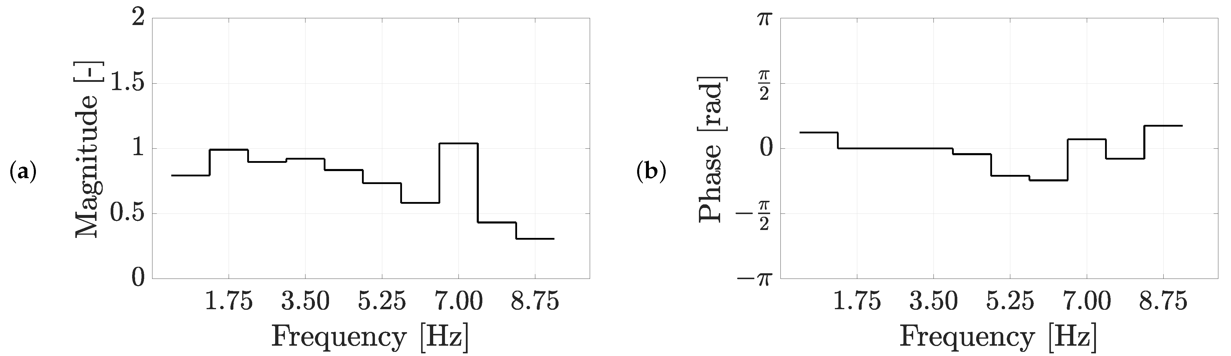
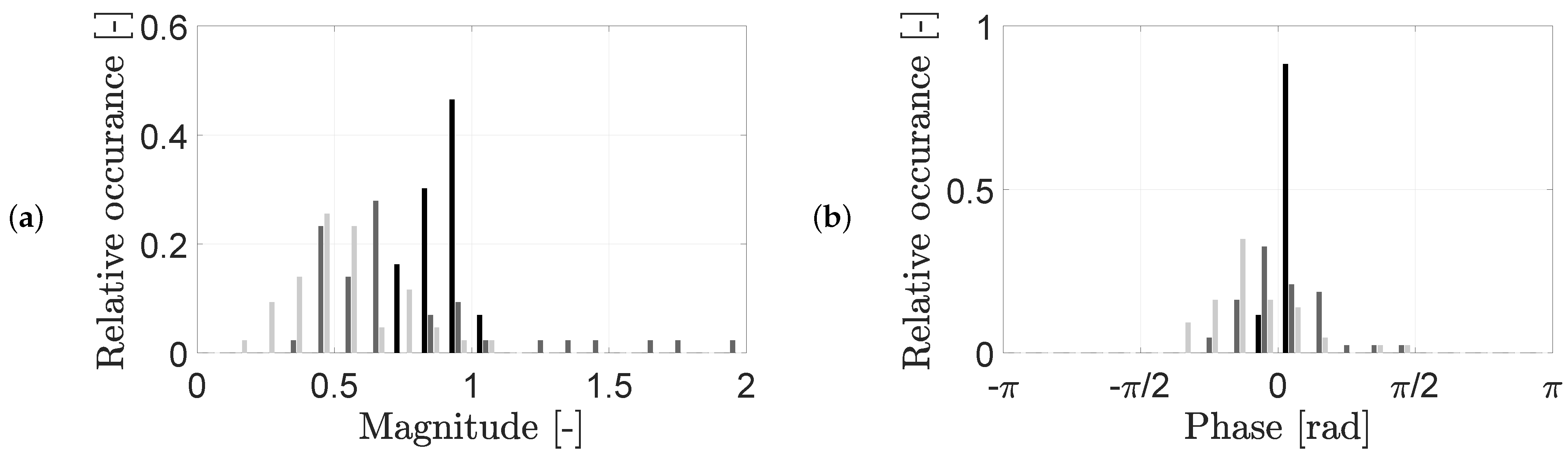
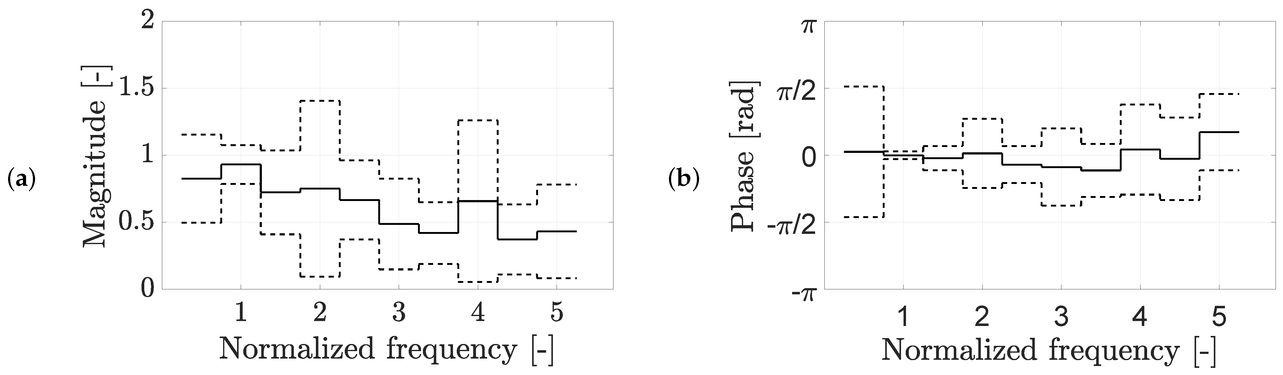
3.3. Modeling the Relation between the Contact Force and the L5 Acceleration
3.4. Contact Force Reconstruction Based on the Registered L5 Acceleration Using the Averaged Transfer Function
3.4.1. Reconstruction Method I
3.4.2. Reconstruction Method II
3.4.3. Reconstruction Method III
3.5. Results of the Force Reconstruction Methodologies
4. Contact Force Reconstruction on Vibrating Surfaces
4.1. Numerical Estimation of the Additional L5 Accelerations Resulting from Human–Structure Interaction
4.2. Contact Force Reconstruction Strategies
4.2.1. Internally-Driven Contact Force Reconstruction Using the Internally-Driven L5 Accelerations
4.2.2. Total Contact Force Reconstruction Using the Total L5 Accelerations
4.2.3. Internally-Driven Contact Force Reconstruction Using the Total L5 Accelerations
4.3. Framework of the Numerical-Experimental Example
- 1.
- The internally-driven contact forces are selected from the registered trials during the laboratory measurements on rigid surfaces (Section 3.1). As the total test duration is longer than the typical trial duration, the contact force and lower-back acceleration vector are repeated. As trials are selected multiple times, a random uniformly-distributed time shift is assigned and sampled from ± the average step period to avoid an artificial correlation between the pedestrians in the crowd. The reason to use the treadmill-identified contact forces and L5 accelerations in the present example instead of the L5 accelerations as collected in the Eeklo Footbridge Benchmark Dataset is twofold. First, only the L5 accelerations are registered in the Eeklo Footbridge Benchmark Dataset, and not the corresponding contact forces. Second, the total L5 accelerations are registered in-situ. It is not possible to extract the internally-driven and mechanical interaction components from the total L5 accelerations. Instead, an estimation of the mechanical interaction component is made by assuming the human body dynamics representing the mechanical HSI can be modeled by an SMD.
- 2.
- The corresponding part of the L5 acceleration as registered during the laboratory experiments is selected and stored in the matrix . This quantity is used to determine the total human body accelerations (step 5) and the contact force reconstruction.
- 3.
- The reference response is calculated by plugging in the internally-driven contact forces in Equation (5). The equation is solved for the modal accelerations and the interaction human body accelerations .
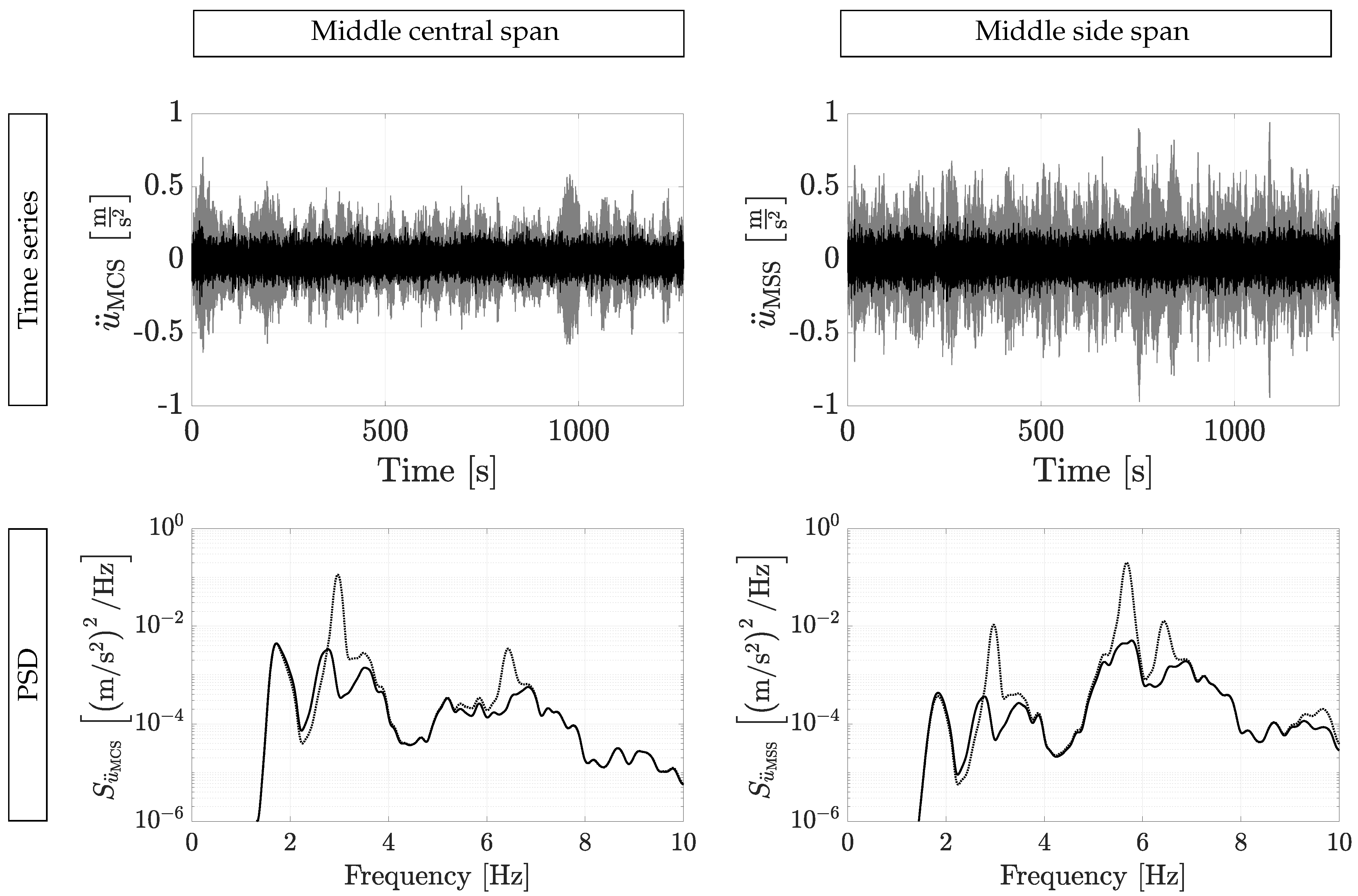
- 4.
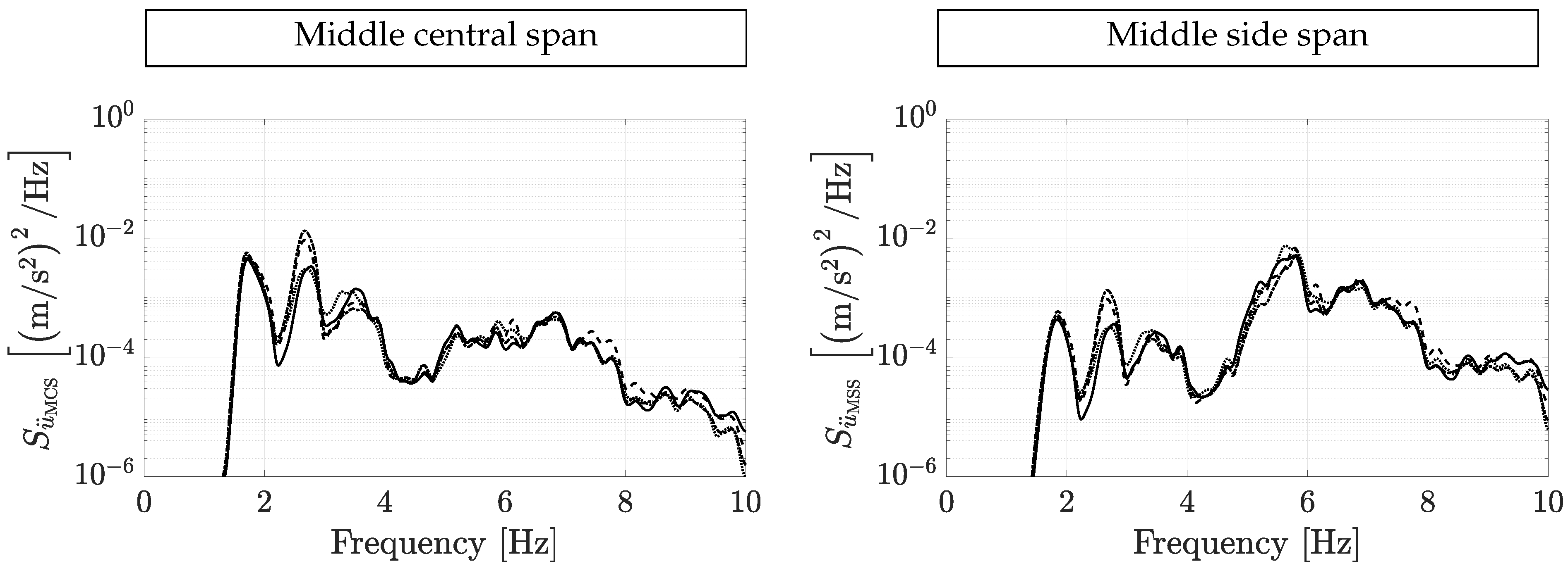
- The modal accelerations are used to calculate the vertical acceleration at the middle of the central span and the middle of the side span . This structural acceleration quantity is hereafter referred to as the reference response.
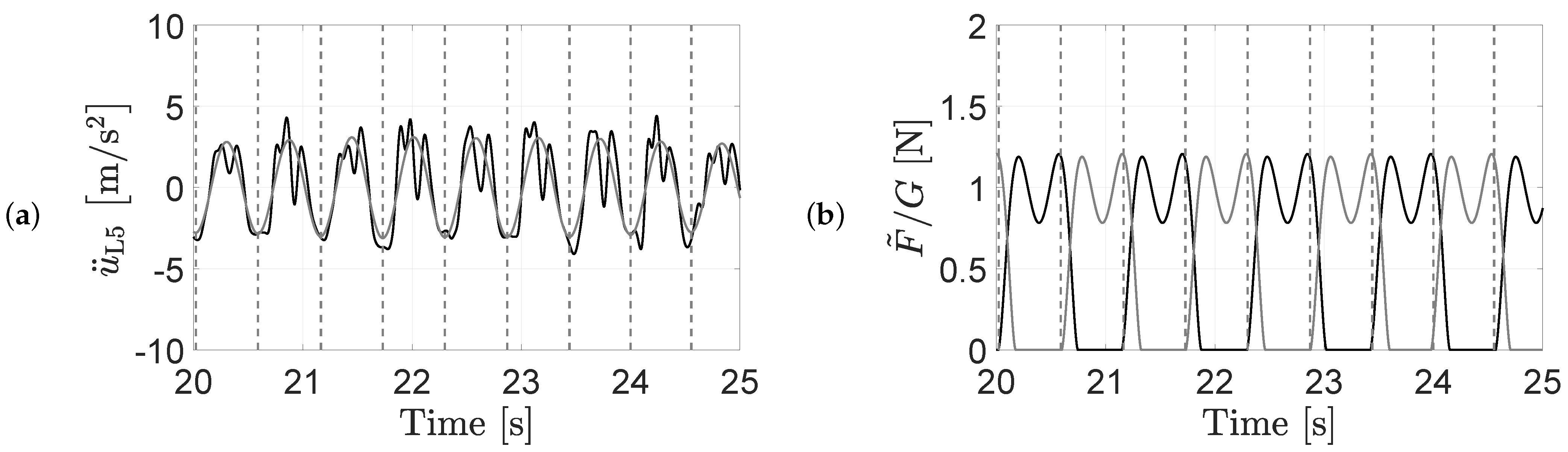
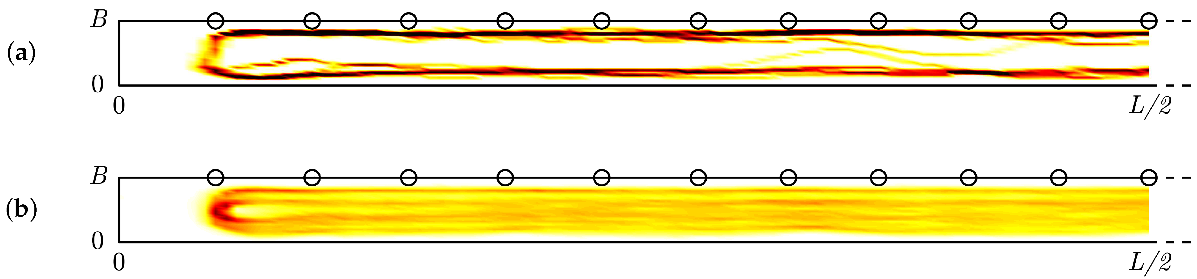
- 5.
- The kinetics of the SMD representing HSI are converted to interaction contact forces and the additional L5 accelerations (Equations (3) and (19)). An example of both quantities is shown in Figure 16. The interaction L5 accelerations are assumed to correspond to the additional kinetics that a pedestrian registers in case of walking on a vibrating surface as a result of the HSI. The total acceleration registered at the lower back is: . This quantity is used for the contact force reconstruction.
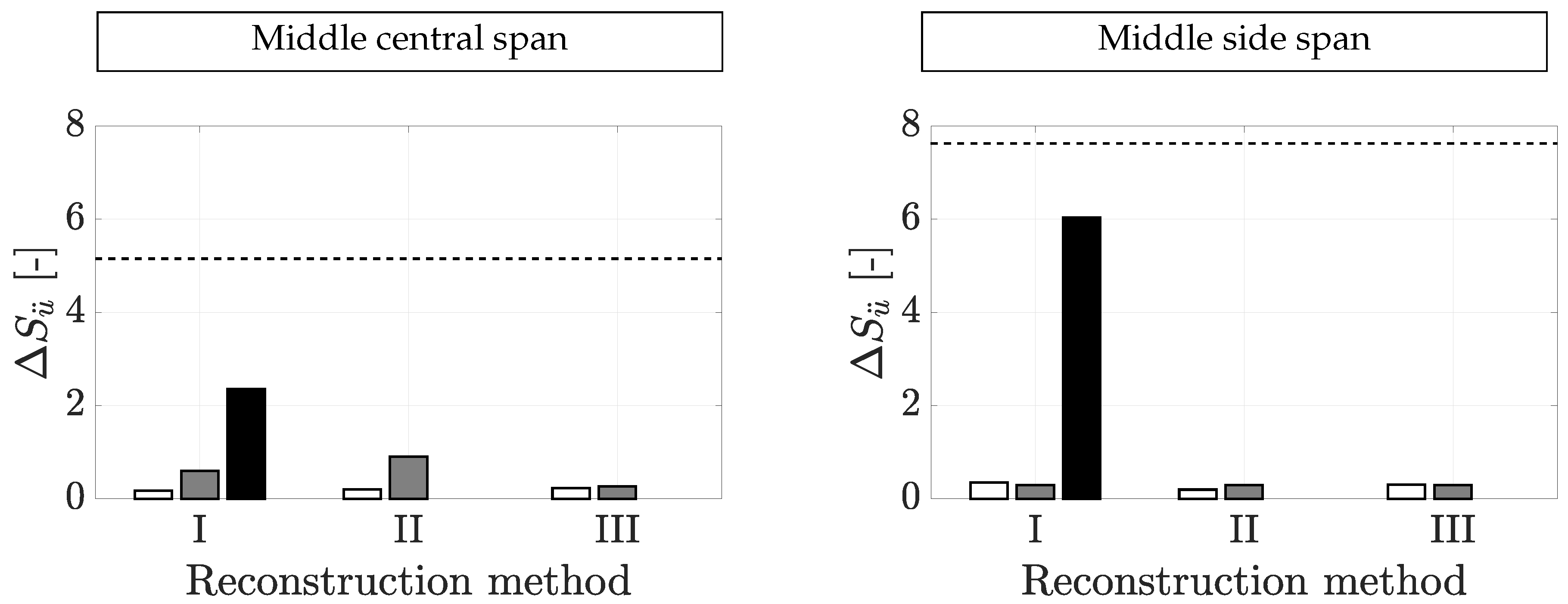
4.4. Results of the Different Reconstruction Scenarios in Vibrating-Surface Conditions
5. Conclusions
Author Contributions
Funding
Institutional Review Board Statement
Informed Consent Statement
Data Availability Statement
Conflicts of Interest
Abbreviations
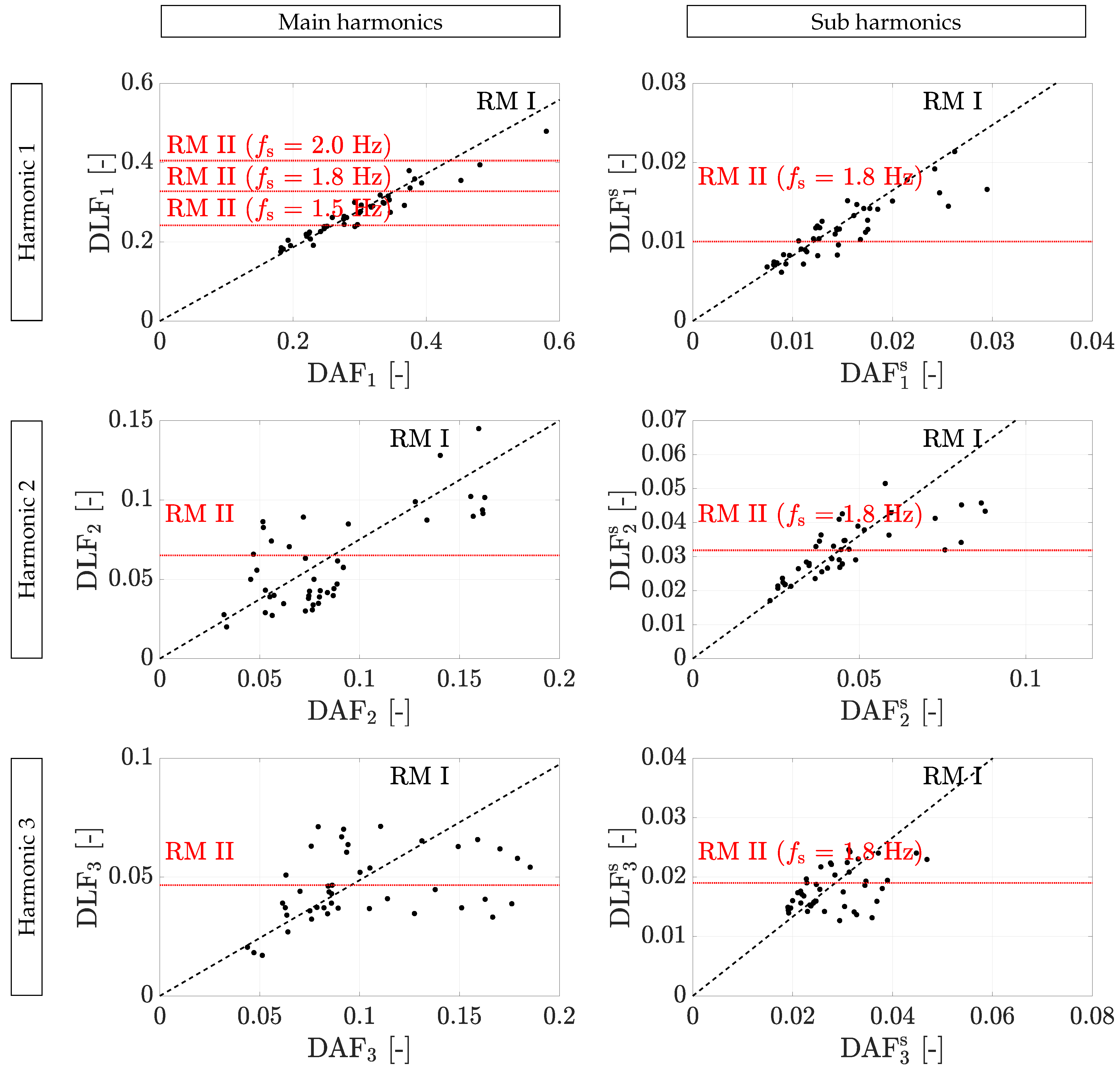
| DAF | Dynamic acceleration factor |
| DLF | Dynamic loading factor |
| HSI | Human–structure interaction |
| L5 | 5th Lumbar vertebra |
| PSD | Power spectral density |
| RM | Reconstruction method |
| SMD | Spring mass damper |
References
- Van Nimmen, K.; Lombaert, G.; De Roeck, G.; Van den Broeck, P. Vibration serviceability of footbridges: Evaluation of the current codes of practice. Eng. Struct. 2014, 59, 448–461. [Google Scholar] [CrossRef]
- Van Nimmen, K.; Lombaert, G.; De Roeck, G.; Van den Broeck, P. The impact of vertical human–structure interaction on the response of footbridges to pedestrian excitation. J. Sound Vib. 2017, 402, 104–121. [Google Scholar] [CrossRef] [Green Version]
- Živanović, S.; Pavic, A.; Reynolds, P. Human-structure dynamic interaction in footbridges. Proc. Inst. Civ. Eng. Bridge Eng. 2005, 158, 165–177. [Google Scholar] [CrossRef]
- Živanović, S.; Pavic, A.; Reynolds, P. Vibration serviceability of footbridges under human-induced excitation: A literature review. J. Sound Vib. 2005, 279, 1–74. [Google Scholar] [CrossRef] [Green Version]
- Association Française de Génie Civil, Sétra/AFGC. Sétra: Evaluation du Comportement Vibratoire des Passerelles Piétonnes Sous L’action des Piétons (Assessment of Vibrational Behaviour of Footbridges Under Pedestrian Loading); AFGC: Paris, France, 2006. [Google Scholar]
- Heinemeyer, C.; Butz, C.; Keil, A.; Schlaich, M.; Goldack, A.; Lukić, M.; Chabrolin, B.; Lemaire, A.; Martin, P.; Cunha, A.; et al. Design of Lightweight Footbridges for Human Induced Vibrations; EUR 23984 EN; European Commission: Luxembourg, 2009. [Google Scholar]
- Živanović, S. Benchmark footbridge for vibration serviceability assessment under vertical component of pedestrian load. J. Struct. Eng. 2012, 138, 1193–1202. [Google Scholar] [CrossRef] [Green Version]
- Van Nimmen, K.; Van Hauwermeiren, J.; Van den Broeck, P. The Eeklo footbridge: Benchmark dataset on pedestrian-induced vibrations. J. Bridge Eng. 2021. forthcoming. [Google Scholar] [CrossRef]
- Bocian, M.; Brownjohn, J.M.; Racic, V.; Hester, D.; Quattrone, A.; Gilbert, L.; Beasley, R. Time-dependent spectral analysis of interactions within groups of walking pedestrians and vertical structural motion using wavelets. Mech. Syst. Signal Process. 2018, 105, 502–523. [Google Scholar] [CrossRef]
- Bocian, M.; Brownjohn, J.M.; Racic, V.; Hester, D.; Quattrone, A.; Monnickendam, R. A framework for experimental determination of localised vertical pedestrian forces on full-scale structures using wireless attitude and heading reference systems. J. Sound Vib. 2016, 376, 217–243. [Google Scholar] [CrossRef] [Green Version]
- Toso, M.A.; Gomes, H.M.; Da Silva, F.T.; Pimentel, R.L. Experimentally fitted biodynamic models for pedestrian-structure interaction in walking situations. Mech. Syst. Signal Process. 2016, 72–73, 590–606. [Google Scholar] [CrossRef]
- Shahabpoor, E.; Pavic, A. Estimation of vertical walking ground reaction force in real-life environments using single IMU sensor. J. Biomech. 2018, 79, 181–190. [Google Scholar] [CrossRef] [PubMed]
- Van Nimmen, K.; Zhao, G.; Seyfarth, A.; Van den Broeck, P. A Robust Methodology for the Reconstruction of the Vertical Pedestrian-Induced Load from the Registered Body Motion. Vibration 2018, 1, 18. [Google Scholar] [CrossRef] [Green Version]
- Guo, Y.; Storm, F.; Zhao, Y.; Billings, S.A.; Pavic, A.; Mazzà, C.; Guo, L.Z. A new proxy measurement algorithm with application to the estimation of vertical ground reaction forces using wearable sensors. Sensors 2017, 17, 2181. [Google Scholar] [CrossRef] [PubMed]
- Denoth, J. Chapter: Load on the locomotor system and modelling. In Biomechanics of Running Shoes; Nigg, B., Ed.; Human Kinetics Publishers: Champaign, IL, USA, 1986; pp. 63–116. [Google Scholar]
- Racic, V.; Brownjohn, J.M.W.; Pavic, A. Reproduction and application of human bouncing and jumping forces from visual marker data. J. Sound Vib. 2010, 329, 3397–3416. [Google Scholar] [CrossRef]
- Van Nimmen, K.; Lombaert, G.; Jonkers, I.; De Roeck, G.; Van den Broeck, P. Characterisation of walking loads by 3D inertial motion tracking. J. Sound Vib. 2014, 333, 5212–5226. [Google Scholar] [CrossRef] [Green Version]
- Ahmadi, E.; Caprani, C.; Živanović, S.; Evans, N.; Heidarpour, A. A framework for quantification of human–structure interaction in vertical direction. J. Sound Vib. 2018, 432, 351–372. [Google Scholar] [CrossRef] [Green Version]
- Matsumoto, Y.; Griffin, M.J. Mathematical models for the apparent masses of standing subjects exposed to vertical whole-body vibration. J. Sound Vib. 2003, 260, 431–451. [Google Scholar] [CrossRef]
- Vasilatoua, V.; Harrisona, R.; Nikitasb, N. Development of a human–structure dynamic interaction model for human sway for use in permanent grandstand design. In Proceedings of the 10th International Conference on Structural Dynamics, EURODYN 2017, Rome, Italy, 10–13 September 2017; Vestroni, F., Romeo, F., Gattulli, V., Eds.; Elsevier: Amsterdam, The Netherlands, 2017; pp. 1877–7058. [Google Scholar] [CrossRef]
- Winter, D.A. The Biomechanics and Motor Control of Human Gait; University of Waterloo Press: Waterloo, ON, Canada, 1988; Volume 74, p. 94. [Google Scholar] [CrossRef]
- Brownjohn, J.M.W. Energy dissipation from vibration floor slabs due to human–structure interaction. J. Shock Vib. 2001, 8, 315–323. [Google Scholar] [CrossRef]
- Zheng, X.; Brownjohn, J.M.W. Modelling and simulation of human-floor system under vertical vibration. In Smart Structures and Materials 2001: Smart Structures and Integrated Systems; Davis, L., Ed.; International Society for Optics and Photonics: Bellingham, WA, USA, 2001; Volume 4327, pp. 513–520. [Google Scholar]
- Duysens, J.; Jonkers, I.; Verschueren, S. MALL: Movement & posture Analysis Laboratory Leuven; Interdepartmental Research Laboratory at the Faculty of Kinisiology and Rehabilitation Sciences-KU Leuven: Leuven, Belgium, 2019. [Google Scholar]
- Vicon Motion Systems. Vicon Motion Systems Product Manuals; Vicon Motion Systems: Los Angeles, CA, USA, 2019. [Google Scholar]
- Živanović, S.; Pavić, A.; Reynolds, P. Probability-based prediction of multi-mode vibration response to walking excitation. Eng. Struct. 2007, 29, 942–954. [Google Scholar] [CrossRef]
- MATLAB. R2016b; The MathWorks Inc.: Natick, MA, USA, 2016. [Google Scholar]
- Gulf Coast Data Concepts. X16-1D: User manual rev B; GCDC LLC: Waveland, MS, USA, 2016. [Google Scholar]
- Xsens Technologies B.V. In MTw User Manual; Xsens: Enschede, The Netherlands, 2010.
- Butz, C. Beutrag zur Berechnung fussgängerinduzierter Brückenschwingungen—Shaker Verlag (Contribution to the Determination of Pedestrian Induced Bridge Vibrations). Ph.D. Thesis, RWTH Aachen, Aachen, Germany, 2006. [Google Scholar]
- McDonald, M.G.; Živanović, S. Measuring Ground Reaction Force and Quantifying Variability in Jumping and Bobbing Actions. J. Struct. Eng. 2017, 143, 1–14. [Google Scholar] [CrossRef]
- Van Hauwermeiren, J.; Van Nimmen, K.; Van den Broeck, P.; Vergauwen, M. Vision-Based Methodology for Characterizing the Flow of a High-Density Crowd on Footbridges: Strategy and Application. Infrastructures 2020, 5, 51. [Google Scholar] [CrossRef]


| Participant | Gender | Age [years] | Height [m] | Mass [kg] | Treadmill Speeds [km/h] |
|---|---|---|---|---|---|
| 1 | male | 25 | 1.82 | 77 | 4.00, 4.50, 5.00 |
| 2 | male | 22 | 1.77 | 72 | 4.00, 4.50, 5.00 |
| 3 | male | 51 | 1.75 | 77 | 4.00, 4.50, 5.00 |
| 4 | male | 27 | 1.89 | 72 | 4.00, 4.50, 5.00 |
| 5 | male | 28 | 1.90 | 85 | 4.00, 4.50, 5.00 |
| 6 | female | 32 | 1.66 | 54 | 4.00, 4.50, 5.00 |
| 7 | male | 24 | 1.80 | 61 | 4.00, 4.50, 5.00 |
| 8 | male | 24 | 1.87 | 82 | 4.25, 4.75, 5.25 |
| 9 | male | 24 | 1.85 | 79 | 4.50, 5.00, 5.50 |
| 10 | male | 24 | 1.73 | 71 | 4.00, 5.00, 5.50 |
| 11 | male | 21 | 1.85 | 78 | 4.25, 5.25, 5.75 |
| 12 | male | 22 | 1.85 | 77 | 4.50, 5.00, 6.00 |
| 13 | male | 22 | 1.65 | 74 | 4.00, 4.50, 5.00 |
| 14 | female | 23 | 1.71 | 70 | 4.25, 4.75, 5.25 |
| 15 | male | 21 | 1.77 | 81 | 4.50, 5.25, 6.00 |
| Mean | 26 | 1.79 | 74.0 | 4.70 | |
| Standard deviation | 7.5 | 0.08 | 8.0 | 0.60 |
| Main Harmonics | Sub Harmonics | |||||||||
|---|---|---|---|---|---|---|---|---|---|---|
| 1 | 2 | 3 | 4 | 5 | 1 | 2 | 3 | 4 | 5 | |
| CC | 0.96 | 0.73 | 0.36 | 0.46 | 0.40 | 0.89 | 0.76 | 0.46 | 0.76 | 0.63 |
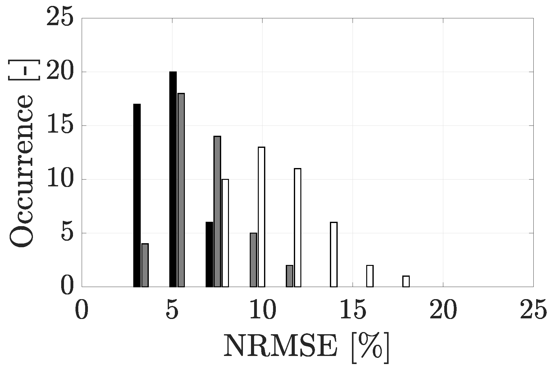
| Frequency Content | 0 Hz–10 Hz | Main Harmonics | Sub Harmonics | ||||||||
|---|---|---|---|---|---|---|---|---|---|---|---|
| 1 | 2 | 3 | 4 | 5 | 1 | 2 | 3 | 4 | 5 | ||
| RM I | 5 | 3 | 10 | 12 | 19 | 16 | 4 | 7 | 10 | 13 | 16 |
| RM II | 7 | 6 | 14 | 12 | 16 | 14 | 4 | 8 | 10 | 12 | 13 |
| RM III | 11 | 9 | 25 | 22 | 16 | 21 | 8 | 19 | 19 | 20 | 19 |
Publisher’s Note: MDPI stays neutral with regard to jurisdictional claims in published maps and institutional affiliations. |
© 2021 by the authors. Licensee MDPI, Basel, Switzerland. This article is an open access article distributed under the terms and conditions of the Creative Commons Attribution (CC BY) license (http://creativecommons.org/licenses/by/4.0/).
Share and Cite
Van Hauwermeiren, J.; Van Nimmen, K.; Vanwanseele, B.; Van den Broeck, P. Contact Force Reconstruction from the Lower-Back Accelerations during Walking on Vibrating Surfaces. Vibration 2021, 4, 205-231. https://0-doi-org.brum.beds.ac.uk/10.3390/vibration4010015
Van Hauwermeiren J, Van Nimmen K, Vanwanseele B, Van den Broeck P. Contact Force Reconstruction from the Lower-Back Accelerations during Walking on Vibrating Surfaces. Vibration. 2021; 4(1):205-231. https://0-doi-org.brum.beds.ac.uk/10.3390/vibration4010015
Chicago/Turabian StyleVan Hauwermeiren, Jeroen, Katrien Van Nimmen, Benedicte Vanwanseele, and Peter Van den Broeck. 2021. "Contact Force Reconstruction from the Lower-Back Accelerations during Walking on Vibrating Surfaces" Vibration 4, no. 1: 205-231. https://0-doi-org.brum.beds.ac.uk/10.3390/vibration4010015