To Investigate the Flow Structure of Discontinuous Vegetation Patches of Two Vertically Different Layers in an Open Channel

Abstract

In the present study, the flow structure of discontinuous double-layered vegetation patches was investigated using a 3D Reynolds stress turbulence model (RSM). The channel domain was built using GAMBIT (Geometry and Mesh Building Intelligent Toolkit). For the simulation and postprocessing, FLUENT (ANSYS) was used to analyze the distribution of the mean velocity, Reynolds stresses, and other flow properties against two different flow conditions. The results captured by the turbulence model at specific locations and the cross section are presented in the form of various velocity profiles and contour plots. In the gap portion, the velocity was visibly lower than that in the vegetation areas, while the influence of patch distribution was not visible in the overlying flow layer. The velocity profiles at critical locations were categorized by numerous modulation points and velocity projections close to the bed, principally for positions straight after the vegetation structures. A distinction in the velocity at the topmost of the smaller vegetation structure was prominent. Reynolds stresses, turbulent kinetic energy, and turbulence intensity exhibited large fluctuations inside the vegetation regions and just behind the vegetation structures compared with in the gap regions.

1. Introduction

Aquatic vegetation considerably decreases mean stream velocities as compared with nonvegetated zones [1]. The existence of discontinued vegetation in the aquatic atmosphere significantly changes the turbulent flow in rivers and streams. Vegetation in usual streams is dispersed in patches that intermingle with the water flow in an intensely nonlinear way. The growing configuration of such patches is affected by the water flow. On the other hand, these patches change flow by influencing flow opposition, sediment conveyance, wave energy, and water quality. The existence of such rough (e.g., discontinued and layered) vegetation alters the flow structure and velocity distribution. Thus, optimum conditions for flow within the vegetation are vital for decreasing the water velocity.

In marine ecologies, vegetation patches perform a vital role. They can reduce wave energy and hinder local fluxes. Thus, vegetation patches are proficient in shielding swamp zones from erosion. Patchy vegetation provides a favorable habitat and species assortment, and generates areas of improved or reduced bed shear stresses [2,3]. With the straight acceptance of nutrients, creation of oxygen, and the detention of suspended deposits, immersed vegetation patches may affect the quality of water [4].

The influences of vegetation on flow features have been examined by a number of investigators using numerical models. The effects of discontinuous immersed vegetation patches on flow turbulence in an open channel were investigated by Zhao et al. [5] using a large eddy simulation (LES) model. An analytical model was proposed by Huai et al. [6] for analyzing the dissemination of streamwise velocity in an open waterway with double-layered vegetation. Previous researchers have proposed numerical models for vegetation in open channel flows. For example, Yokojima et al. [7] investigated flow in an open channel with cylindrical vegetation structures. They analyzed various patch configurations with the help of an LES model. Kamel et al. [8] developed a k-epsilon (k-ε) model to predict the flow in meandering-type open channels. Jalonen et al. [9] determined the characteristics of vegetation areas by flood plain flow modeling. Huai et al. [10] analyzed the interaction of flows with rigid vegetation and investigated the effects of vegetation patches on flow by utilizing an LES model. Ghisalberti and Nepf [11] conducted an experimental and numerical study in order to predict the mean velocity profiles of shear layers generated by vegetation. Their study presented a one-dimensional approximation to the three-dimensional flow. Jarvela [12] performed an experimental investigation to analyze the flow structure in the presence of flexible vegetation, whereas the patterns of flow partially obstructed by rigid vegetation were elucidated by Ben Meftah et al. [13]. Zeng et al. [14] utilized a 3D Reynolds averaged Navier–Stokes model including the Spalart–Allmaras turbulence closure to reproduce the flow progress inside a vegetation patch. They investigated the flow properties through vegetation patches experimentally and numerically. A numerical investigation of flow through inflexible nonsubmerged vegetation was proposed by Kim et al. [15] by implementing a large eddy simulation model. A numerical examination of flow in a multistage compound waterway with vegetation was proposed by Wen et al. [16]. In his research work, turbulence properties were investigated by applying a k-ε turbulence model. Xia and Nehal [17] and Shih et al. [18] experimentally investigated the features of flow in an open channel with vegetation. They used various arrangements of vegetation and investigated hydraulic characteristics in open channel flows. A large eddy simulation (LES) model was implemented by Lu et al. [19] in order to analyze turbulence features like Reynolds stresses inside the vegetation concentration and to investigate the influence of immersed vegetation on solute conveyance in an open canal. Mossa and De Serio [20] and Mossa et al. [21] analyzed the turbulent jets in an obstructed flow with emergent vegetation and Mossa et al. [21] proved the enhancement of turbulent intensity and the transverse deflection of flow around the individual cylinders. The flow structure in a channel partially obstructed by rigid emergent vegetation was also investigated by Ben Meftah and Mossa [22]. In recent research works, flow properties and turbulence features of flows in vegetated domains have received significant consideration. The models discussed above are for vegetated streams with constant vegetation elevation and formation. Detailed information regarding discontinuous and layered vegetation patches collectively is not yet available, though they are more common in natural rivers and make the flow–vegetation interaction more complicated. In the regular riparian condition, vegetation has distinctive elevations and formations. In a high flood situation, both the smaller and the larger vegetation will be immersed; when the flood is not all that extensive, the shorter vegetation is submerged and the larger is emerged. Throughout this circumstance, the communication between the larger layer and the smaller layer with discontinuity in patches will result in a very unique distribution of velocities and Reynolds stresses.

The objective of this study is to build up a numerical model to analyze the flow properties, like mean velocity profiles and turbulence characteristics, through discontinuous vegetation patches of two vertically different layers in an open channel flow. The research work is also focused on analyzing the influence of discontinued double-layered vegetation patches on the distribution of flow.

2. Materials and Methods

2.1. Mathematical Model and Governing Equations

For steady incompressible flow in an open channel, continuity and Reynolds-averaged Navier–Stokes (RANS) equations are employed, which can be written as:

$$\frac{\partial U_i}{\partial x_i}=0,$$

(1)

$$U_j\frac{\partial }{\partial x_j}(U_i)=\frac{\nu }{\rho }\frac{\partial }{\partial x_j}\left(\frac{\partial U_i}{\partial x_j}+\frac{\partial U_j}{\partial x_i}\right)-\frac{1}{\rho }\frac{\partial P}{\partial x_i}+F_i+\left(-\overline{u_i{u}_j}\right),$$

(2)

where U_i is the component of velocity in the $x_i$ direction. For Equation (2), $U_j$ is the component of velocity in the $x_j$ direction, $\nu$ is the kinematic viscosity, $\rho$ is the density of water, $P$ is the pressure, $F_i$ is external force, and $u_i{u}_j$ are the Reynolds stresses.

The Reynolds stress model (RSM) is the advanced kind of RANS turbulence models [23,24]. Equation (3) is the general form for the transport of Reynolds stresses including various terms. Each term represents the partial differential equation used for the transport of independent Reynolds stresses. The equation for the Reynolds stresses transport [25] can be written as

$$\frac{\partial R_{ij}}{\partial t}+C_{ij}=P_{ij}+D_{ij}-{\epsilon }_{ij}+{{\displaystyle \prod }}_{ij}+{\mathsf{\Omega }}_{ij}$$

(3)

where $R_{ij}$ is the rate of change of Reynolds stresses, $C_{ij}$ is the transport of convection, $P_{ij}$ is the rate of production of Reynolds stresses, $D_{ij}$ is the transport of stresses by diffusion, ${\epsilon }_{ij}$ is dissipation rate of stresses, ${{\displaystyle \prod }}_{ij}$ is stresses transport due to turbulent pressure–strain interactions, and ${\mathsf{\Omega }}_{ij}$ is the transport of stresses due to rotation.

The turbulence kinetic energy for obtaining the boundary conditions of the Reynolds stresses is modeled using Equation (4):

$$\frac{\partial }{\partial t}\left(\rho k\right)+\frac{\partial }{\partial x_i}\left(\rho k{u}_i\right)=\frac{\partial }{\partial x_j}\left[\left(\mu +\frac{{\mu }_t}{{\sigma }_k}\right)\frac{\partial k}{\partial x_j}\right]+\frac{1}{2}\left[P_{ii}+G_{ii}\right]-\rho \epsilon \left(1+2M_t^2\right)+S_k$$

(4)

where $k$ is the tensor for kinetic energy, $\epsilon$ is the dissipation rate, ${\mu }_t$ is the turbulent viscosity, ${\sigma }_k$ = 0.82, and $S_k$ is a user-defined source term.

Also, the turbulence kinetic energy tensor (k) for a specific factor can be modeled as

$$k=\frac{1}{2}\overline{u_i^{\prime }{u}_i^{\prime }}.$$

(5)

Equation (6) models the scalar dissipation rate $\left(\epsilon \right)$ as

$$\frac{\partial }{\partial t}\left(\rho \epsilon \right)+\frac{\partial }{\partial x_i}\left(\rho \epsilon u_i\right)=\frac{\partial }{\partial x_j}\left[\left(\mu +\frac{{\mu }_t}{{\sigma }_{\epsilon }}\right)\frac{\partial \epsilon }{\partial x_j}\right]C_{\epsilon 1}\frac{1}{2}\left[P_{ii}+C_{\epsilon 3}{G}_{ii}\right]\frac{\epsilon }{k}-C_{\epsilon 2}\rho \frac{{\epsilon }^2}{k}+S_{\epsilon }$$

(6)

where ${\sigma }_{\epsilon }$ = 1.0, $C_{\epsilon 1}$ = 1.44, $C_{\epsilon 2}$ = 1.92, and $S_{\epsilon }$ is a user-defined source term. $C_{\epsilon 3}$ is obtained with respect to the following relation [26]:

$$C_{\epsilon 3}=\tan h\left|\frac{v}{u}\right|$$

(7)

where v is the component of flow velocity along the gravitational vector and u is the component of flow velocity transverse to the gravitational vector.

Also, the dissipation tensor (${\epsilon }_{ij}$) for a specific factor can be modeled by

$${\epsilon }_{ij}=\frac{2}{3}{\delta }_{ij}\rho \epsilon .$$

(8)

The turbulent viscosity for the Reynolds stress model is computed using

$${\mu }_t=\rho C_{\mu }\frac{k^2}{\epsilon }$$

(9)

where $C_{\mu }$ = 0.09.

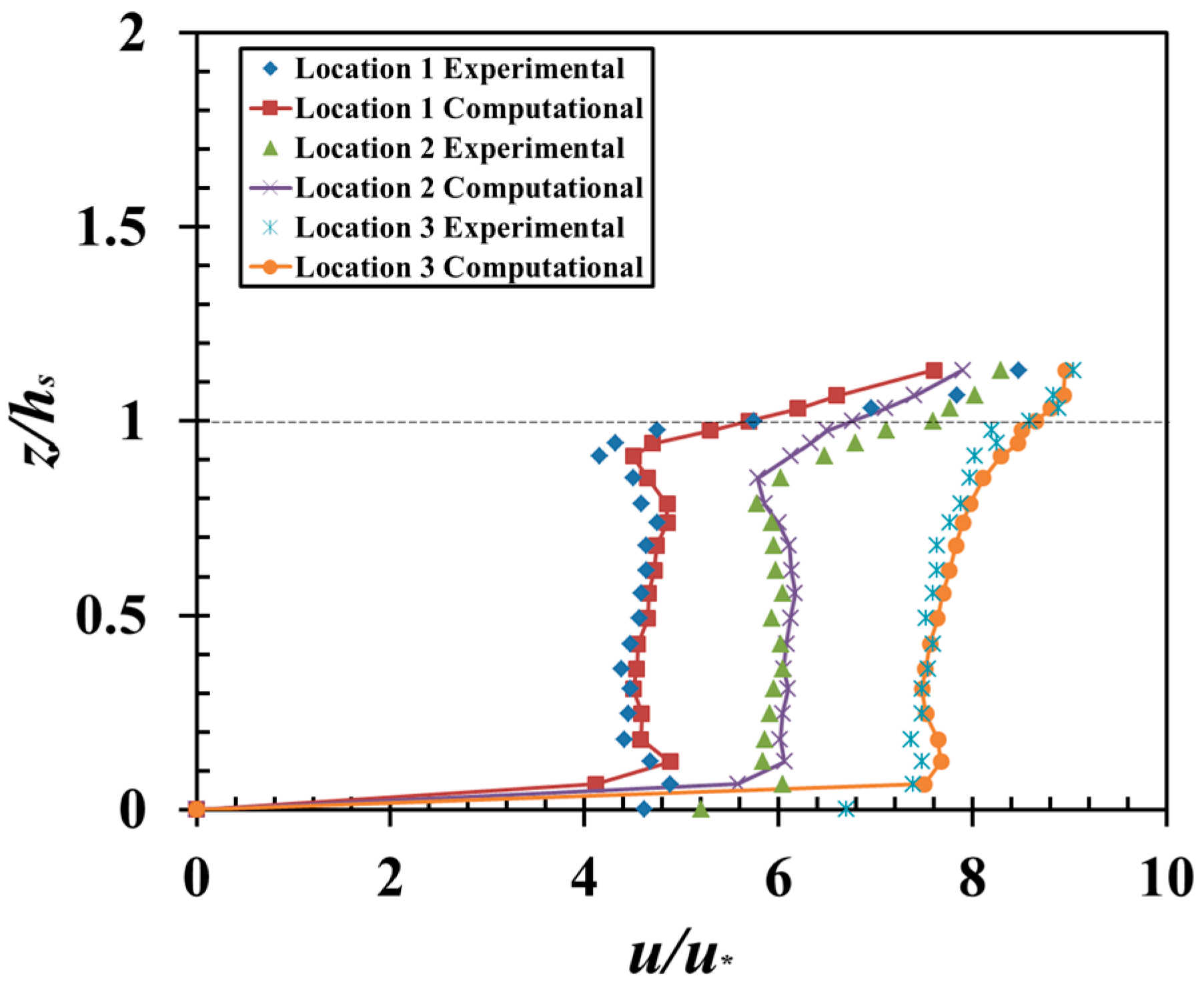
2.2. Validation of Numerical Model

The experimental data of Liu et al. [27] has been used for validation of the numerical model. Liu et al. [27] performed experiments in a 4.3 m long and 0.3 m wide plexiglass recirculating domain with a slope of 0.003. The vegetation test segment was 3 m long, and was fastened to the base 1.3 m from the entry of the channel. Experiment number six of Liu et al. [27], with double-layered rigid vegetation of diameter (d) 0.635 cm, was adopted for simulating the current numerical model. The heights of the larger and shorter vegetation used in the experiment were 76 and 152 mm, respectively, with a spacing of s_s/d = 8 and s_t/d = 16 organized in linear and staggered patterns. The flow capacity percentages engaged by the vegetation for the equivalent spacings were 2.86 and 0.35 for the lined and 0.60 and 0.18 for the staggered patterns. The flow conditions of the experiment performed by Liu et al. [27] for double-layered vegetation are summarized in

Table 1. Hydraulic conditions (Liu et al. [27]), where h_t and h_s are the taller and shorter vegetation heights, S_t/d and S_s/d are the larger (linear) and smaller (staggered) vegetation spacings, Q is the discharge, z is the water depth, U_avg is the average velocity, u* = (gzS)^1/2 is the shear velocity, where g = 9.81 m/s² and S = slope, F_r is the Froude number, R_e is the cylinder Reynolds number, and R_e* is the flow Reynolds number.

ht (cm)	hs (cm)	St/d	Ss/d	Q (L/s)	z (cm)	Uavg (m/s)	u* (m/s)	Fr	Re	Re*
15.2	7.6	16	8	11.4	9.22	0.424	0.0521	0.446	2700	38,500

.

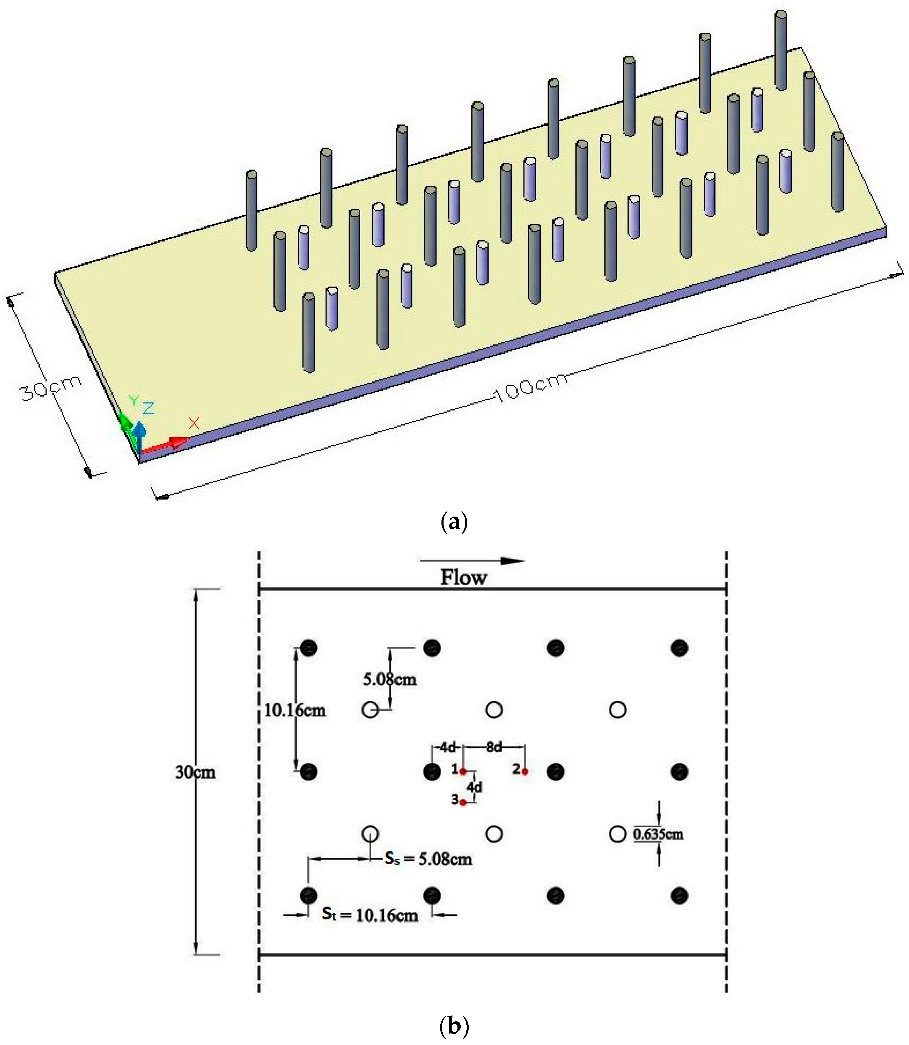
2.3. Setup and Boundary Conditions

In the current experimental model, simplification of geometry was needed due to the smaller vegetation size and large mesh structure. Only a part of the whole domain, i.e., 1.0 m long, comprising double-layered rigid vegetation was modeled in GAMBIT with all the other dimensions kept the same (Figure 1a,b). In order to achieve the flow–structure interaction, the vegetation was simulated in the form of solid circular cylinders. A tri-pave mesh with tetrahedral elements was used in this simulation. The mesh used had 400 × 120 × 40 nodes in the streamwise, lateral, and vertical directions, giving 1.92 million grid points. To ensure uniformity all over the flume, a periodic boundary condition was introduced to the computational domain that offered an interface between the inlet and outlet faces (translational periodicity). The following boundary conditions were incorporated in the model: (i) periodic boundary condition at inlet/outlet; (ii) symmetry condition at free surface; and (iii) domain walls, i.e., side walls and bed of the channel as well as vegetation walls were regarded as nonslip walls.

The meshed model of the domain was imported to 3D commercial CFD (Computational Fluid Dynamics) software FLUENT for simulation and postprocessing. The pressure–velocity coupling was achieved through the SIMPLE algorithm. The standard values of under-relaxation factors were utilized in the simulation process. The calculation was thought to have converged after all the residuals reached 1 × 10⁻⁶. The standard wall function was used as a near wall treatment. Turbulence closure was achieved with a Reynolds stress model. The computational time consumed by the normal computer in this simulation work was around 16–18 h. A mesh independence trial was directed by doubling the nodes in the crosswise and depthwise directions. However, no noteworthy dissimilarity was noticed in the outcomes due to refinement of the mesh. The alteration in primary velocity values due to the mesh refinement was less than 1%, which indicated that the results are mesh-independent.

The simulated results of the normalized mean velocity along the normalized vertical depth at specified positions were compared with the experimental results as shown in Figure 2. The velocity profiles in Figure 2 show that the simulated results are close to the experimental results. This demonstrates the validity of the numerical model.

2.4. Conditions for Numerical Simulation

The numerical model of this study included a part of the experimental channel with length 1.8 m and discontinued vegetation patches, while all other dimensions were kept the same. The schematic diagram of the domain model is shown in Figure 3a,b, while the critical locations in the last vegetation patch are shown in Figure 3c. The critical locations are located just upstream and downstream of the vegetation structures as a larger amount of turbulence exists at these locations. These critical locations (just before and after the vegetation structures) are also investigated by Liu et al. [27].

The tetrahedral mesh used had 720 × 120 × 40 nodes in the streamwise, lateral, and vertical directions, giving 3.5 million grid points. A conventional mass flow rate at the periodic boundary was provided equal to 11.4 L/s for Case A and 25 L/s for Case B. All other boundary conditions were kept the same. The hydraulic conditions for the two cases are summarized in

Table 2. Hydraulic conditions for simulation, where h_t and h_s are the taller and shorter vegetation heights, S_t/d and S_s/d are the larger (linear) and smaller (staggered) vegetation spacings, Q is the discharge, z is the water depth, U = Q/A is the velocity, F_r is the Froude number, R_e is the cylinder Reynolds number, and R_e* is the flow Reynolds number.

Case	ht (cm)	hs (cm)	St/d	Ss/d	Q (L/s)	z (cm)	U (m/s)	Fr	Re	Re*
A	15.2	7.6	16	8	11.4	9.22	0.412	0.446	2700	38,500
B	15.2	7.6	16	8	25	14	0.596	0.509	3760	82,900

.

3. Results and Discussion

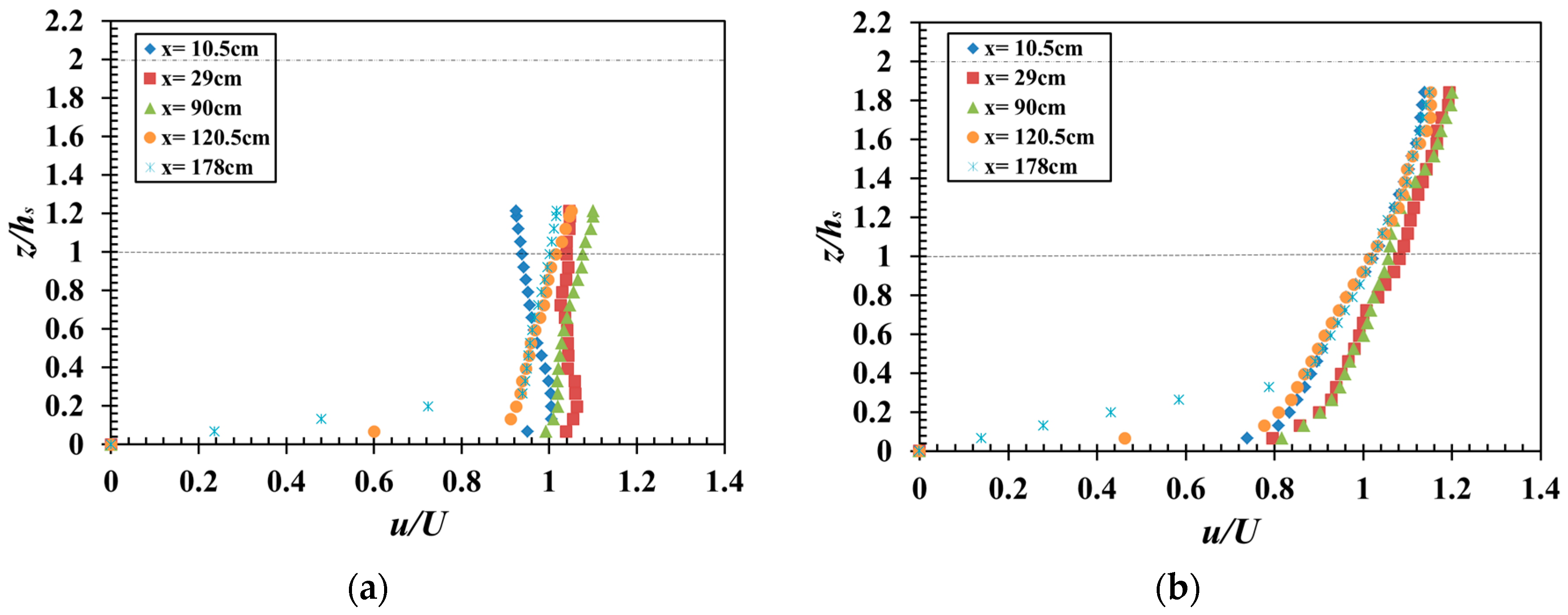
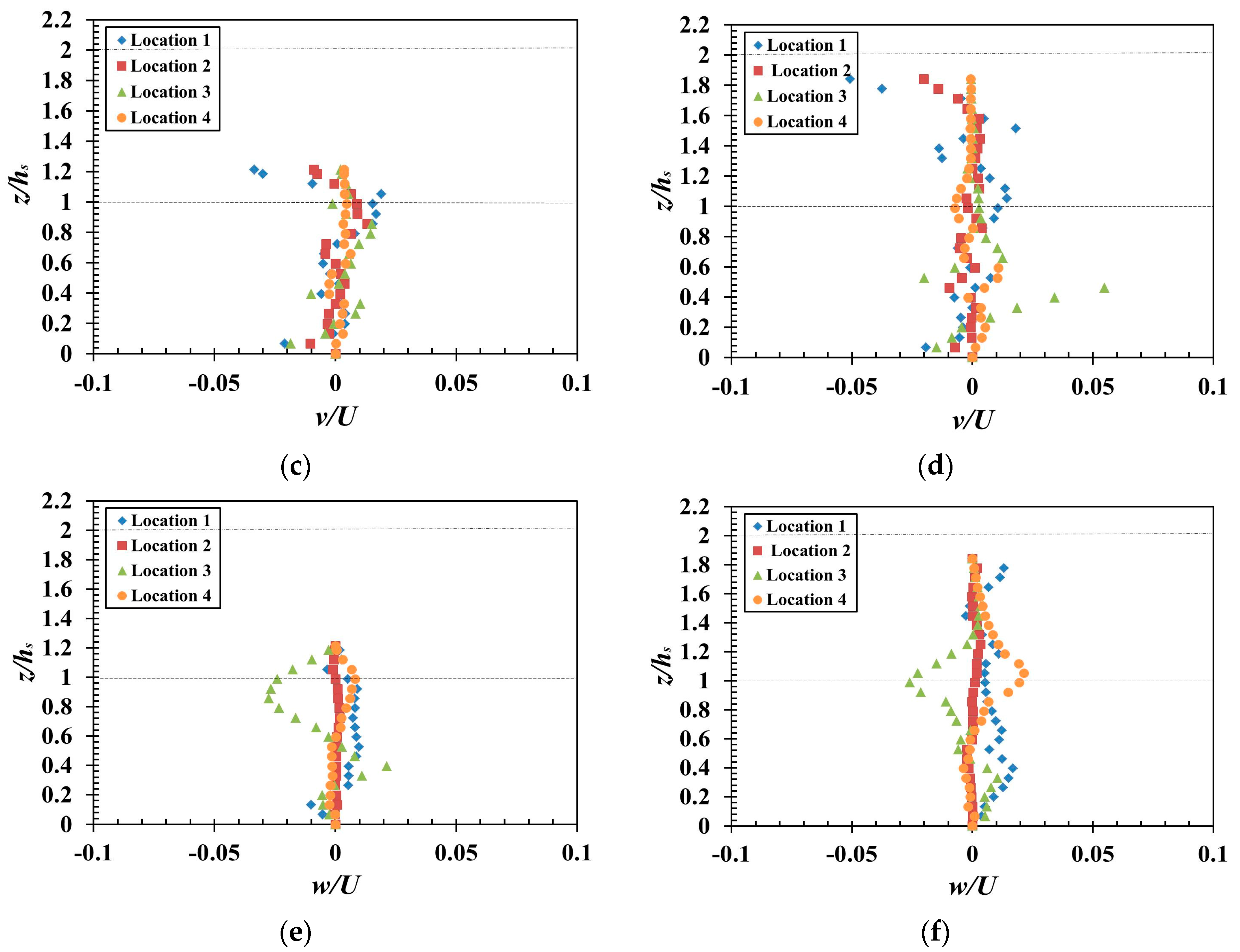
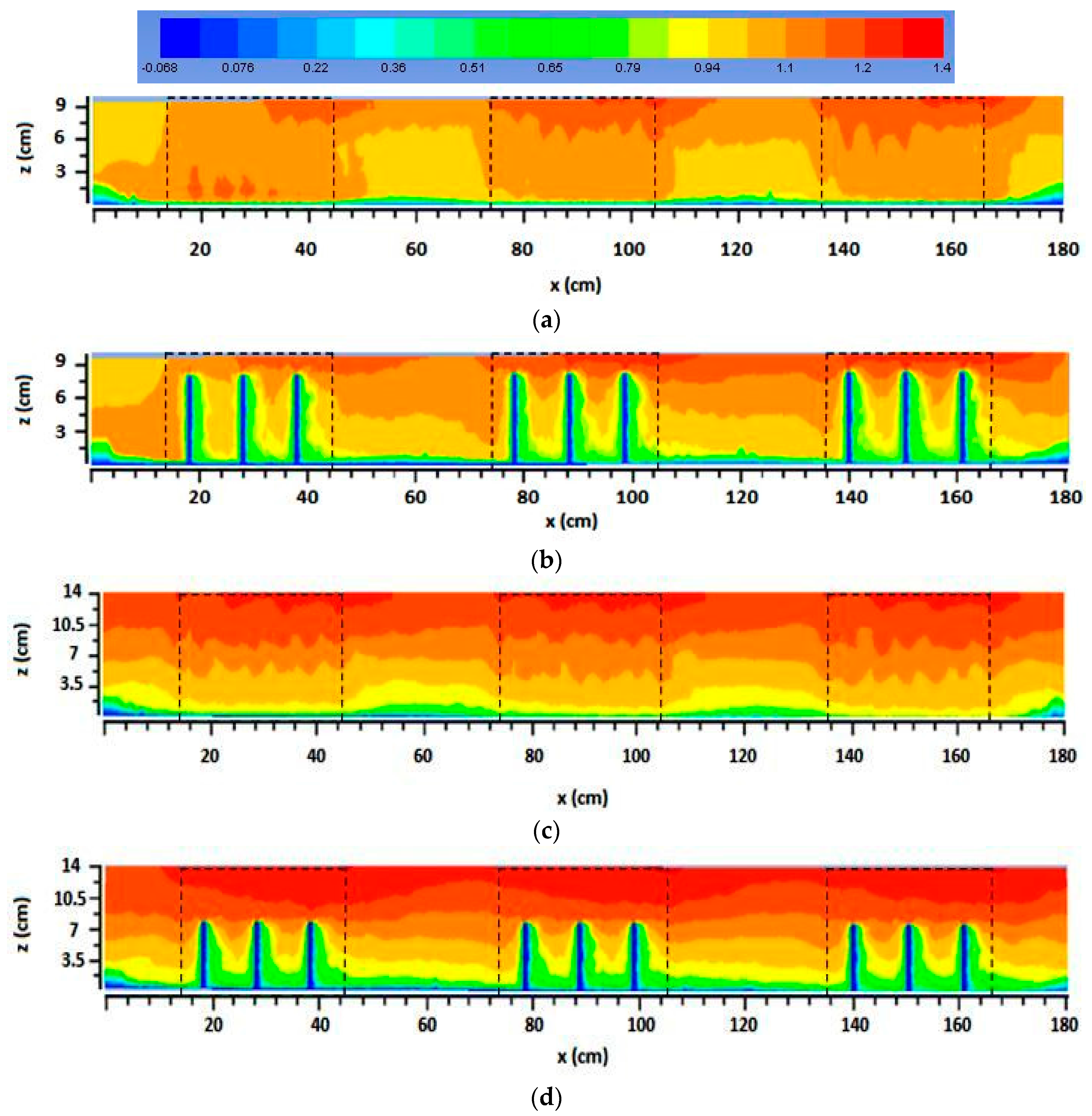
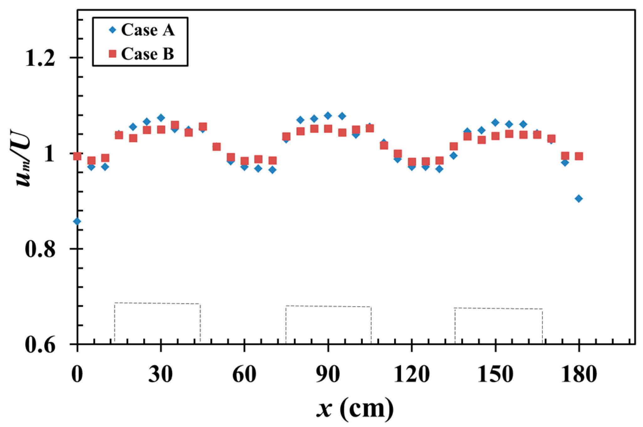
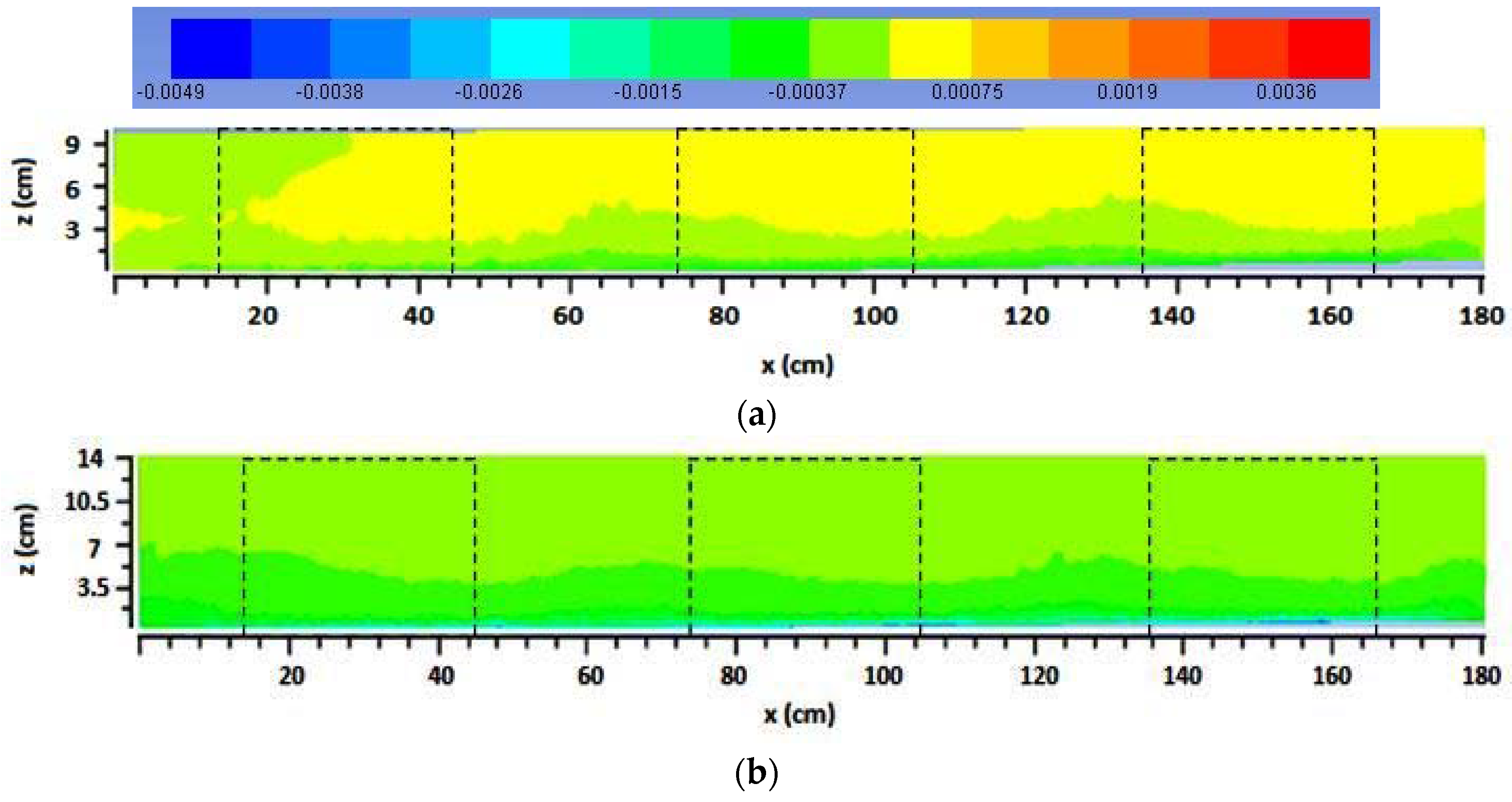
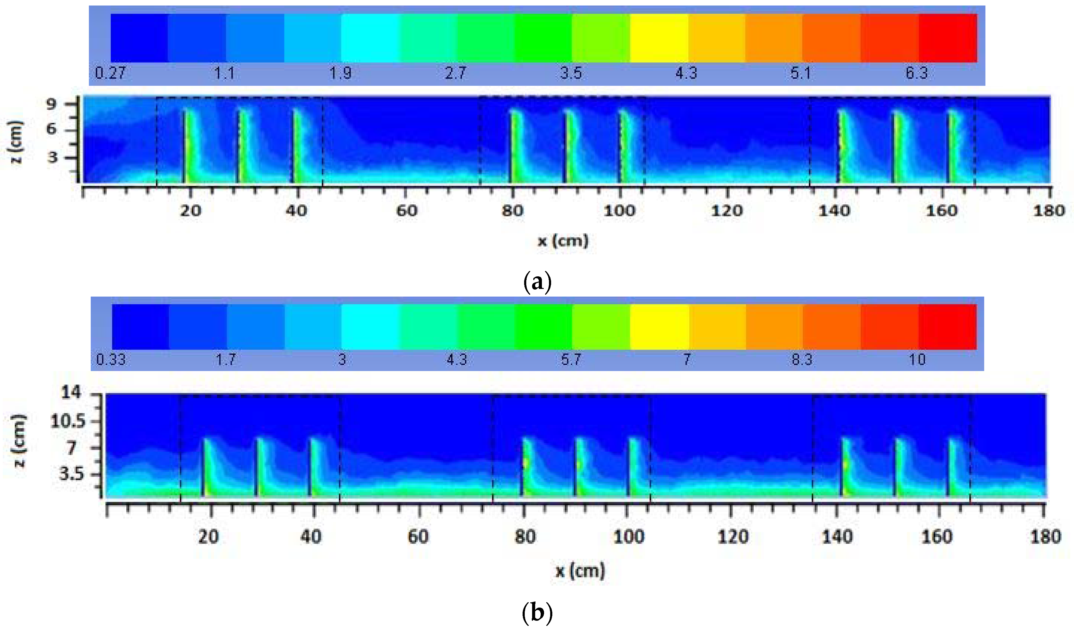
3.1. Mean Flow Characteristics

A longitudinal cross section at y = 17.54 cm from the boundary between the taller and shorter cylinders (i.e., y = 20.08 and y = 15 cm) was adopted primarily as the distance of 2.54 cm from the center path in the y direction is comparatively suitable to avoid the major effect of the wake after each structure (Figure 3c). Velocity profiles with the short dowels submerged and large dowels nonsubmerged at cross section y = 17.54 cm for various positions of both cases are shown in Figure 4. The velocities were made nondimensional according to U and the channel depth was normalized with respect to the smaller vegetation height “h_s”. The upper dashed line denotes the larger vegetation height “h_t”, whereas the lower dashed line denotes the smaller vegetation height “h_s” correspondingly.

The normalized velocity profile of Case B (Figure 4b) is significantly reduced below the smaller submerged vegetation height and varies more above it comparative to the mean velocity profile of Case A (Figure 4a). The longitudinal mean velocity values for Case B are 8% less than those for Case A within the patches (i.e., x = 29 and 90 cm). The mean values of velocity for Case B are 5% less than those of Case A for the gaps below the vegetation height (i.e., x = 10.5 and 120.5 cm) which can be visualized in Figure 4. Both cases show that velocity is reduced inside the patches (z < h_s) past the interruption area, while the velocity is amplified comparative to the preliminary flow velocity inside the overlying flow (z > h_s). In Figure 4b, the velocity above the smaller vegetation is significantly faster than the velocity within it because of the sparser arrangement of the larger vegetation and higher depth of flow. Due to the exchange of momentum between the smaller and larger vegetation structures, the velocity profile is not constant throughout the depth of flow.

The difference among the mean velocity profiles at various locations of both cases (Figure 4a,b) is not clear at section y = 17.54 cm, as there was no direct effect of larger or smaller vegetation structures. Therefore, various critical locations were selected for measuring flow characteristics. The critical locations are marked in Figure 3c. Takemura and Tanaka [28] proved that the computing position can be a significant feature while observing the flow configuration of vegetated flow. The velocity profiles (for both Case A and Case B) at these typical locations are prominent. In Figure 5, “u” is the velocity component in the x (streamwise) direction, “v” is the velocity component in the y (transverse) direction, and “w” is the velocity component in the z (vertical) direction. The streamwise velocities directly upstream of vegetation structures (Locations 2 and 4) are almost in between the largest velocities and smallest fluctuations, whereas velocities in the region (at a distance of 4d) immediately behind the vegetation structures (Locations 1 and 3) exhibits smaller velocities and larger fluctuations (Figure 5a,b).

In Figure 5a,b, at Location 2, the velocity is almost constant above the bed region as this position is located upstream of taller vegetation structures. However, for other critical locations positioned downstream of vegetation, i.e., Locations 1 and 3, the fluctuations in the magnitudes of velocity are observed. A sudden rise in velocity close to the top of the shorter submerged vegetation structures can be witnessed at Locations 3 and 4 which are located just upstream and downstream of smaller vegetation structures. This sudden rise is more clearly visible for Case B. The velocity profile for Case A reveals a rapid modulation point at z/h_s = 0.8, directly beneath the top of the shorter vegetation, because of the arrangement of the larger vegetation organization (s_t/d = 16) and small amount of submergence of the shorter vegetation. An inflection point at z/h_s = 0.6 for Case B is observed due to high submergence of the short dowels.

The velocities orthogonal to the streamwise directions, i.e., v and w components (Figure 5c–f) are low compared with the velocities in the streamwise direction (Figure 5a,b). Almost zero or negative magnitudes of velocities in the y and z directions are observed at all the critical locations. The flow is strongly deflected in the transverse and vertical directions at Location 3 as compared to other critical locations (Figure 5c–f). Similar to the streamwise velocity component, the transverse and vertical components of velocity also showed larger fluctuations downstream of vegetation structures (Locations 1 and 3) as compared to locations upstream of vegetation (Locations 2 and 4).

Overall, very small vertical velocities (w) are observed at all critical locations for both Case A and Case B (Figure 5e,f), whereas relatively large values of vertical velocity behind the larger vegetation structure (Location 1) indicate considerable upward movement of the fluid. In addition, maximum vertical downward flows occurred at the top, i.e., z/h_s = 1, of the smaller submerged vegetation structure for Cases A and B (a negative velocity shows downward flow at Location 3 in Figure 5e,f).

The contours of the normalized longitudinal velocity on the y = 17.54 cm longitudinal plane for Cases A and B are shown in Figure 6a,c, respectively. Similarly, contour plots at section y = 20.08 cm passing through the array of smaller vegetation structures are also captured as shown in Figure 6b,d. The flows reveal noteworthy variations when they reach the patches. A clear optimum connection is present between the velocity enlargement and the initial flow velocity for the overlying flow (z > h_s). Similar to the velocity profiles (Figure 4a,b) of both cases, the contour plots of the mean velocity at section y = 17.54 cm (Figure 6a,c) show an inflection point at the top of the submerged vegetation structures, and higher velocity magnitudes above the smaller vegetation structures can be witnessed with respect to the lower zone of submerged vegetation. Also, the velocity magnitudes in the gap zones are slightly lower than those in the vegetation patch zones. The contour plots captured by the numerical model show that the velocity normally remains constant upstream and downstream of the vegetation patch. For both the discharges, the velocity is greatly affected within the vicinity of vegetation. It is visible that the velocity has maximum value above the vegetation zone. Hector Barrios-Pina et al. [29], in their numerical investigation through double-layered vegetation, also found that the flow velocity rises above the vegetated region.

Near the bed, a minor descending current constituent occurs which can be witnessed in all contours of Figure 6. This is primarily because of the abrupt difference in the obstruction at the boundary of the vegetation patch. The covering influence of the patches results in a reduction of velocity within the gap areas as compared to that within the patch areas. Hence, the velocity difference among the vegetated zones and nonvegetated zones is quite significant.

Figure 7 shows that the flow is nonuniform when it reaches the patches, while it is consistent upstream and downstream of the patches. The depth-averaged mean velocities of Figure 7 are plotted at a distance of 17.54 cm from the boundary (Figure 3c). The patches range from 13.8 to 30.48 cm, 74.76 to 105.24 cm, and 135.72 to 166.2 cm on the horizontal axis of Figure 7 for both Case A and Case B. The dimensionless depth-averaged mean velocity is considerably larger in the patch areas than in the gap areas for both the cases. The same results were found by Zhao et al. [5] in their research work of discontinuous vegetation patches. The rising velocities in the patches are rational due to the hindering effect of patches. The effect of patches lasts for a definite distance past the downstream verge; hence, the mean velocity profiles flop to regain their usual shapes. The food source and physical atmosphere of the gap districts are appropriate for aquatic creatures, from a biological perspective. In these areas, sediments probably get deposited [30,31,32].

3.2. Turbulence Characteristics

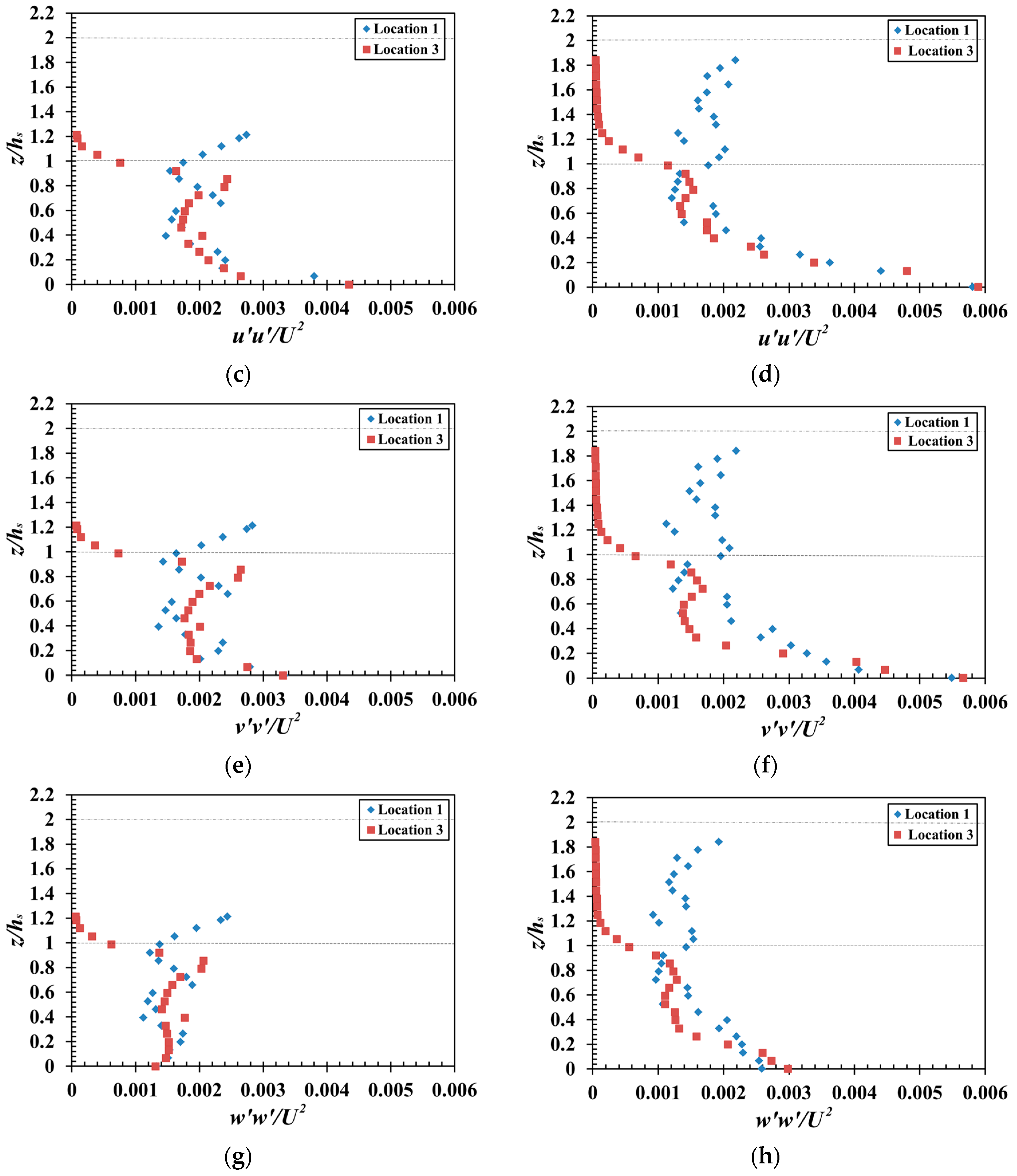
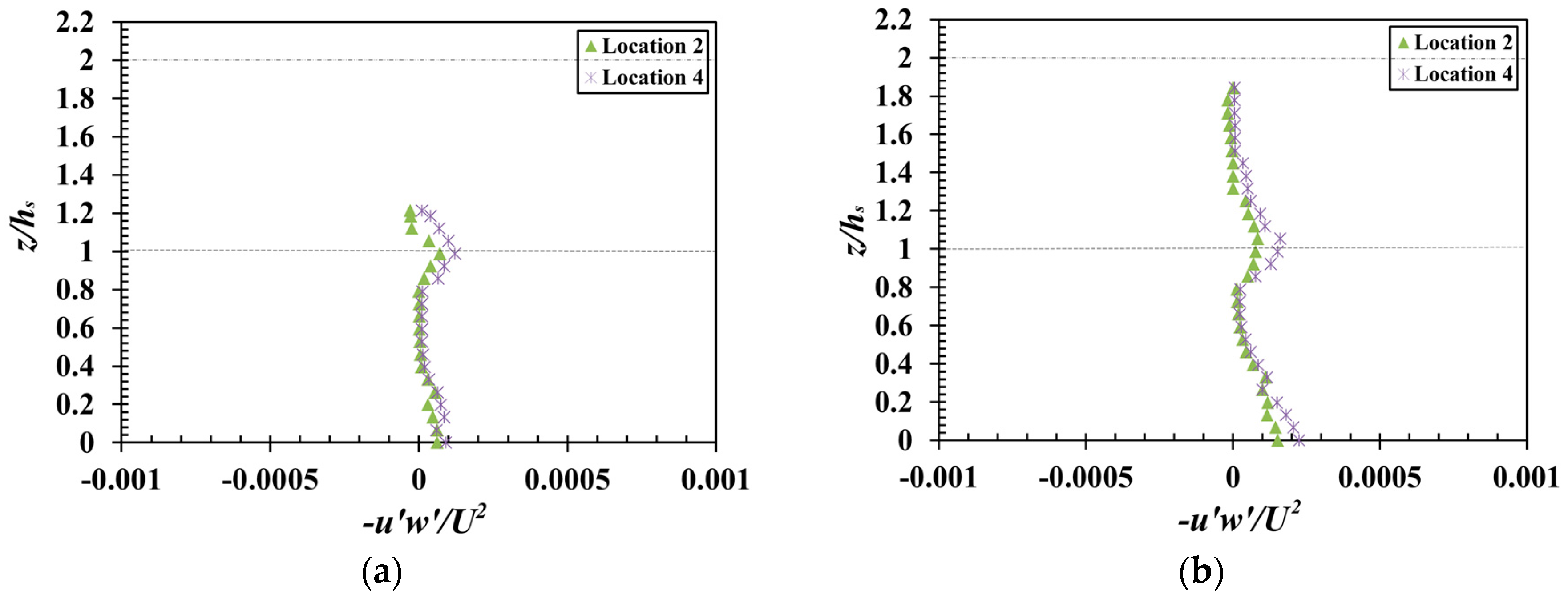
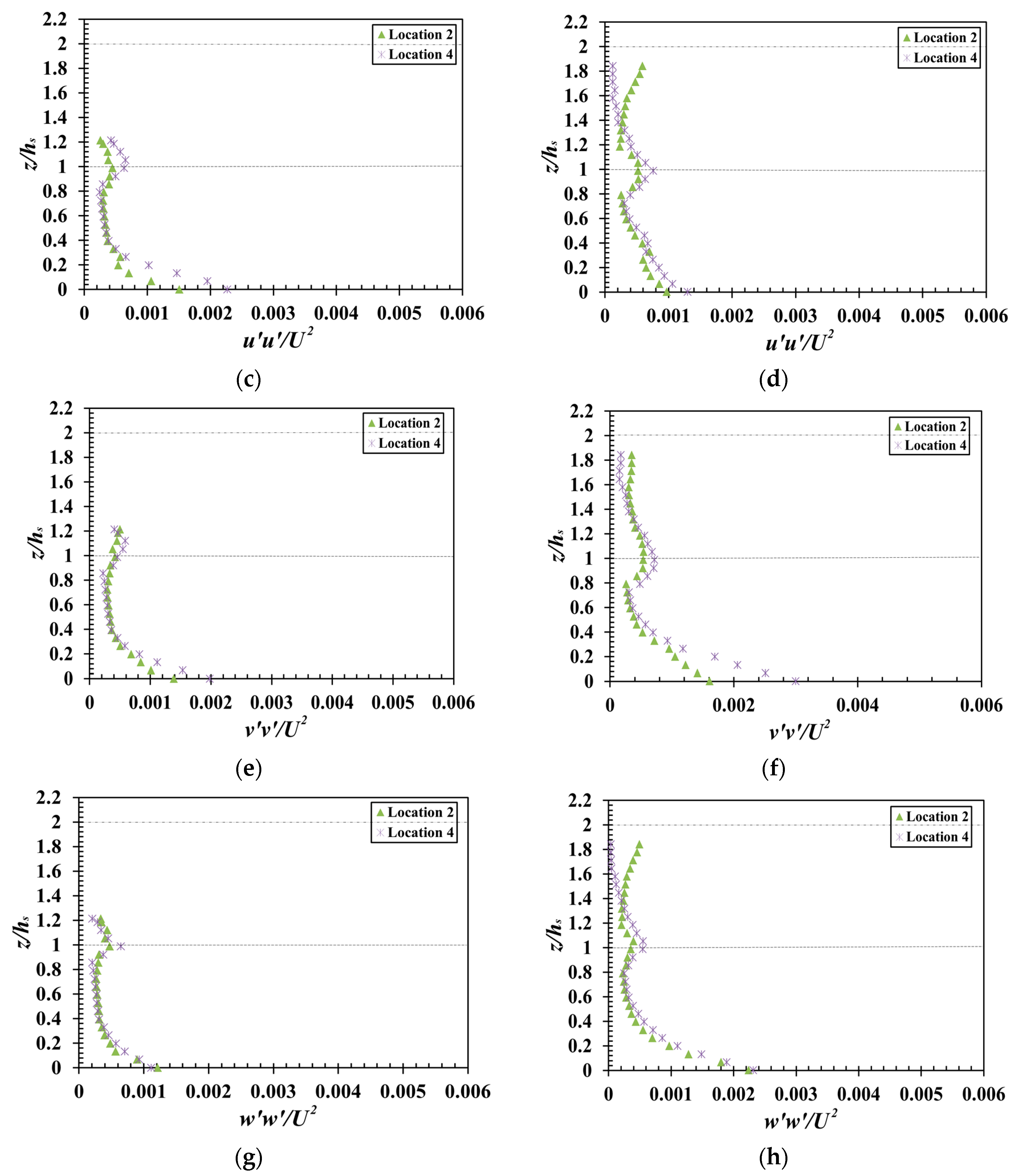
3.2.1. Reynolds Stresses

Reynolds stresses (used to represent turbulence characteristics), including both shear (u’w’) and normal stresses, were investigated at critical locations. These stresses were made nondimensional according to U² and the depth of domain was normalized with the smaller vegetation height “h_s” (as shown in Figure 8). Figure 8 shows the profiles of stresses at critical locations (1 and 3) for both Case A and Case B. In this figure, “u” represents the streamwise variations and “w” represents the variations in the vertical component of the velocity. The Reynolds shear stresses are almost constant while moving from the bed towards the top of the vegetation (Figure 8a,b). An abrupt variation in normal and shear stresses can be witnessed just before the top of the vegetation for both cases. This is due to the fact that larger turbulence occurs at the topmost of the canopy. Negative Reynolds shear stresses are visible near the bed for both Case A and Case B at critical locations 1 and 3. From this, we can conclude that the bed zone inside the patch acquires lesser Reynolds stresses, which may result in the deposition of sediment particles in this zone.

Figure 9 shows the Reynolds shear and normal stresses of both Case A and Case B at Locations 2 and 4, which are less critical as compared with the stresses at Locations 1 and 3. Due to the hindrance offered by the vegetation structures, negative Reynolds shear stresses (u’w’) are witnessed close to the bed, similar to the previous locations (1 and 3). For both Case A and Case B, the stresses at Locations 2 and 4 (Figure 9) show lower fluctuations and turbulence as compared with the stresses at Locations 1 and 3 (Figure 8). From bed to top, the profiles of the normal stresses are almost constant, whereas fluctuations in the values can be witnessed at the top of the smaller submerged vegetation (Figure 9).

The contour plots of Reynolds stresses at section y = 17.54 cm for both cases are shown in Figure 10a,b. The Reynolds stress contour plot is observed to be almost constant. Close to the top of the canopy (z/h_s), the ultimate values of Reynolds stress can be observed, whereas negative stresses are witnessed close to the domain bed. Kelvin–Helmholtz eddies appear regularly on the top of vegetation patches and develop with the downstream length; however, the Reynolds stress is almost definite close to the domain bed and flow surface.

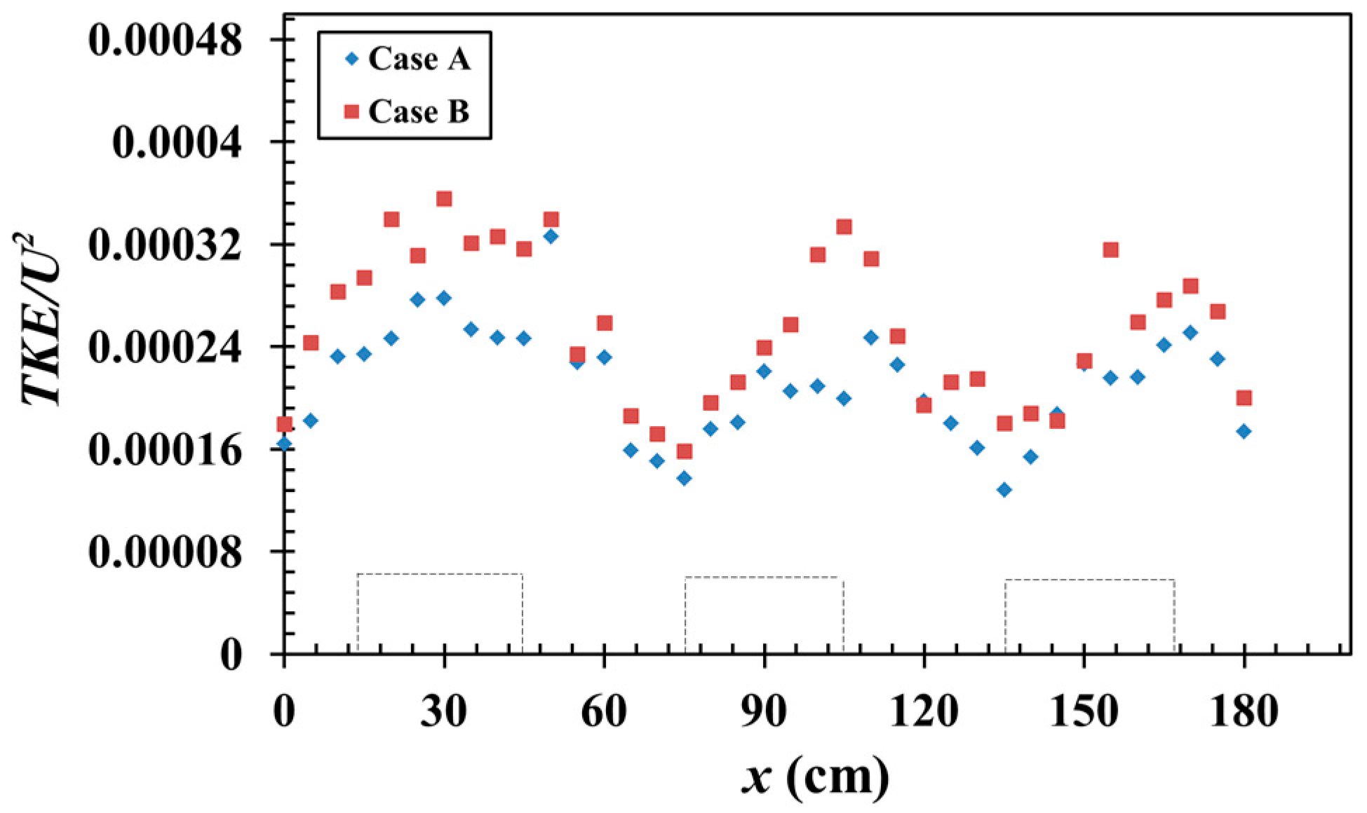
3.2.2. Turbulent Kinetic Energy

Figure 11 shows the deviation of depth-averaged turbulent kinetic energy along the same longitudinal distance of Figure 7. The energy decreases in the gaps but increases in the vegetation regions. A rising trend can be visualized for the depth-averaged kinetic energy. In previous research works, the extreme value of the turbulent energy is witnessed at the topmost of vegetation [5,13]. Among the patch and the gap regions, a visible dissimilarity in values of kinetic energy is present. Also, a significant difference has been observed for both Case A and Case B. The depth-averaged turbulent kinetic energy exhibits sturdier general increments for Case B as compared to Case A. Fast initial flow velocity is primarily responsible for the results of Case B.

3.2.3. Turbulence Intensity

Figure 12a,b shows the profiles of turbulent intensity at critical locations (1, 2, 3, and 4). For both Case A and Case B, low turbulence intensity is witnessed upstream of vegetation structures (Locations 2 and 4), whereas larger turbulence is observed downstream of vegetation structures (Locations 1 and 3) for the depth within the submerged vegetation. Larger turbulence is also observed close to the bed. Case B obtains a larger percentage of turbulence intensity as compared with Case A because of higher discharge and a greater Reynolds number. For Locations 2 and 4, between the tops of the small and large vegetation, the turbulence intensity is almost constant. In this region, the turbulence intensity at Location 3 is significantly higher than that at the other locations. For Locations 3 and 4, large fluctuations and sharp inflections are observed at the top of the submerged vegetation structures (lower dashed line). This is due to the reason that Locations 1 and 3 are located directly behind the vegetation structures.

The turbulence intensity at section y = 20.08 cm is reported in Figure 13 to investigate and characterize the fluctuations in the channel flow with smaller vegetation submerged in water. Figure 13a,b illustrates that Case A has maximum intensity 6.3% and minimum intensity 0.27%, whereas larger turbulence has been observed for Case B with 10% maximum and 0.33% minimum turbulence intensity, respectively. It can be visualized from the contours in Figure 13 that local larger magnitudes of intensity localize closer to the edge of vegetation. Due to the discontinuity and resistance among the vegetated and nonvegetated regions, a sharp slope of turbulence intensity appears overhead and beneath the canopy verge.

4. Conclusions

The response of the flow approaching double-layered discontinuous vegetation in a rectangular open channel has been investigated computationally. A Reynolds stress turbulence model was subsequently employed to replicate the flow development in this research work. The results were analyzed, keeping in mind the effects of both double-layered and discontinuous vegetation patches, in the form of mean stream-wise velocities and Reynolds stresses with various profiles and plots.

• The mean streamwise velocity considerably rises at the top of the vegetation and is almost constant inside the larger and shorter vegetation. A spike in velocity is witnessed close to the bed of the domain and a sharp inflection is observed over the top of the smaller submerged vegetation structures.
• For greater discharge through discontinuous double-layered vegetation patches, streamwise velocity values are 8% less under the submerged vegetation height. On the other hand, for higher discharge through gap regions, the velocity values are 5% less as compared with the lower discharge case.
• Higher velocities were visualized in the vegetation patch regions compared with in the gap regions. This identifies that the gap areas are favorable for deposition of sediments and advantageous for aquatic creatures in terms of physical atmosphere and nourishment.
• Reynolds stresses suffer larger fluctuations above the top of the shorter submerged vegetation structures, whereas for the patch and gap zones, stresses are observed to be low, which may benefit sediment particle deposition. Also, larger turbulence intensity is witnessed for the discharge with a larger Reynolds number.
• The outcomes demonstrated that the flow through discontinuous and double-layered vegetation patches is always nonuniform. This study can be used to enhance understanding of flow features with layered and discontinued vegetation in streams or rivers.

References

1. Shoji, F. Flood-control measure that utilize nation function of river. In Proceedings of the XXV Congress of Inter-Nation Association for Hydraulic Research, Tokyo, Japan, 30 August–3 September 1993; Volume VII. [Google Scholar]
2. Chao, X.; Jia, Y.; Shields, F.D.; Wang, S.S.; Cooper, C.M. Three-dimensional numerical modeling of cohesive sediment transport and wind wave impact in a shallow oxbow lake. Adv. Water Resour. 2008, 31, 1004–1014. [Google Scholar] [CrossRef]
3. Kemp, J.L.; Harper, D.M.; Crosa, G.A. The habitat-scale ecohydraulics of rivers. Ecol. Eng. 2000, 16, 17–29. [Google Scholar] [CrossRef]
4. Keskinkan, O.; Goksu, M.Z.L.; Basibuyuk, M.; Forster, C.F. Heavy metal adsorption properties of a submerged aquatic plant (Ceratophyllum demersum). Bioresour. Technol. 2004, 92, 197–200. [Google Scholar] [CrossRef] [PubMed]
5. Zhao, F.; Huai, W. Hydrodynamics of discontinuous rigid submerged vegetation patches in open-channel flow. J. Hydro-Environ. Res. 2016, 12, 148–160. [Google Scholar] [CrossRef]
6. Huai, W.; Wang, W.; Hu, Y.; Zeng, Y.; Yang, Z. Analytical model of the mean velocity distribution in an open channel with double-layered rigid vegetation. Adv. Water Resour. 2014, 69, 106–113. [Google Scholar] [CrossRef]
7. Yokojima, S.; Kawahara, Y.; Yamamoto, T. Impacts of vegetation configuration on flow structure and resistance in a rectangular open channel. J. Hydro-Environ. Res. 2015, 9, 295–303. [Google Scholar] [CrossRef]
8. Kamel, B.; Ilhem, K.; Ali, F.; Abdelbaki, D. 3D simulation of velocity profile of turbulent flow in open channel with complex geometry. Phys. Procedia 2014, 55, 119–128. [Google Scholar] [CrossRef]
9. Jalonen, J.; Järvelä, J.; Virtanen, J.P.; Vaaja, M.; Kurkela, M.; Hyyppä, H. Determining Characteristic Vegetation Areas by Terrestrial Laser Scanning for Floodplain Flow Modeling. Water 2015, 7, 420–437. [Google Scholar] [CrossRef]
10. Huai, W.; Xue, W.; Qian, Z. Large-eddy simulation of turbulent rectangular open-channel flow with an emergent rigid vegetation patch. Adv. Water Resour. 2015, 80, 30–42. [Google Scholar] [CrossRef]
11. Ghisalberti, M.; Nepf, H.M. The limited growth of vegetated shear layers. Water Resour. Res. 2004, 40, 1–12. [Google Scholar] [CrossRef]
12. Järvelä, J. Effect of submerged flexible vegetation on flow structure and resistance. J. Hydrol. 2005, 307, 233–241. [Google Scholar] [CrossRef]
13. Meftah, M.B.; De Serio, F.; Malcangio, D.; Mossa, M. Resistance and boundary shear in a partly obstructed channel flow. In River Flow 2016; Constantinescu, G., Garcia, M., Hanes, D., Eds.; Taylor & Francis Group: London, UK, 2016; pp. 795–801. [Google Scholar]
14. Zeng, C.; Li, C.W. Measurements and modeling of open-channel flows with finite semi-rigid vegetation patches. Environ. Fluid Mech. 2014, 14, 113–134. [Google Scholar] [CrossRef]
15. Kim, H.S.; Nabi, M.; Kimura, I.; Shimizu, Y. Computational modeling of flow and morphodynamics through rigid-emergent vegetation. Adv. Water Resour. 2015, 84, 64–86. [Google Scholar] [CrossRef]
16. Wen, W.; Huai, W.; Meng, G. Numerical investigation of flow through vegetated multi-stage compound channel. J. Hydrodyn. 2014, 26, 467–473. [Google Scholar]
17. Xia, J.; Nehal, L. Hydraulic Features of Flow through Emergent Bending Aquatic Vegetation in the Riparian Zone. Water 2013, 5, 2080–2093. [Google Scholar] [CrossRef]
18. Shih, S.S.; Hong, S.S.; Chang, T.J. Flume Experiments for Optimizing the Hydraulic Performance of a Deep-Water Wetland Utilizing Emergent Vegetation and Obstructions. Water 2016, 8, 265. [Google Scholar] [CrossRef]
19. Lu, J.; Dai, H.C. Effect of submerged vegetation on solute transport in an open channel using large eddy simulation. Adv. Water Resour. 2016, 97, 87–99. [Google Scholar] [CrossRef]
20. Mossa, M.; De Serio, F. Rethinking the process of detrainment: Jets in obstructed natural flows. Sci. Rep. 2016, 6, 1–11. [Google Scholar] [CrossRef] [PubMed]
21. Mossa, M.; Meftah, M.B.; De Serio, F.; Nepf, H.M. How vegetation in flows modifies the turbulent mixing and spreading of jets. Sci. Rep. 2017, 7, 6587. [Google Scholar] [CrossRef] [PubMed]
22. Ben Meftah, M.; Mossa, M. Partially obstructed channel: Contraction ratio effect on the flow hydrodynamic structure and prediction of the transversal mean velocity profile. J. Hydrol. 2016, 542, 87–100. [Google Scholar] [CrossRef]
23. Launder, B.E. Second-Moment Closure: Present… and Future. Inter. J. Heat Fluid Flow 1989, 10, 282–300. [Google Scholar] [CrossRef]
24. Launder, B.E.; Reece, G.J.; Rodi, W. Progress in the Development of a Reynolds-Stress Turbulence Closure. J. Fluid Mech. 1975, 68, 537–566. [Google Scholar] [CrossRef]
25. Versteeg, H.K.; Malalasekera, W. An Introduction to Computational Fluid Dynamics. Available online: https://ekaoktariyantonugroho.files.wordpress.com/2008/04/an-introduction-to-computational-fluid-dynamics-versteeg.pdf (accessed on 12 January 2018).
26. Henkes, R.A.W.M.; Van Der Vlugt, F.F.; Hoogendoorn, C.J. Natural Convection Flow in a Square Cavity Calculated with Low-Reynolds-Number Turbulence Models. Int. J. Heat Mass Trans. 1991, 34, 1543–1557. [Google Scholar] [CrossRef]
27. Liu, D.; Diplas, P.; Hodges, C.C.; Fairbanks, J.D. Hydrodynamics of flow through double layer rigid vegetation. Geomorphology 2010, 116, 286–296. [Google Scholar] [CrossRef]
28. Takemura, T.; Tanaka, N. Flow structures and drag characteristics of a colony type emergent roughness model mounted on a flat plate in uniform flow. Fluid Dyn. Res. 2007, 39, 694–710. [Google Scholar] [CrossRef]
29. Barrios-Piña, H.; Ramírez-León, H.; Rodríguez-Cuevas, C.; Couder-Castañeda, C. Multilayer Numerical Modeling of Flows through Vegetation Using a Mixing-Length Turbulence Model. Water 2014, 6, 2084–2103. [Google Scholar] [CrossRef]
30. Da Silva, Y.J.A.B.; Cantalice, J.R.B.; Singh, V.P.; Cruz, C.M.C.A.; da Silva Souza, W.L. Sediment transport under the presence and absence of emergent vegetation in a natural alluvial channel from Brazil. Int. J. Sediment Res. 2016. [Google Scholar] [CrossRef]
31. Follett, E.M.; Nepf, H.M. Sediment patterns near a model patch of reedy emergent vegetation. Geomorphology 2012, 179, 141–151. [Google Scholar] [CrossRef]
32. Chao, W.A.N.G.; Zheng, S.S.; Wang, P.F.; Jun, H.O.U. Interactions between vegetation, water flow and sediment transport: A review. J. Hydrodyn. 2015, 27, 24–37. [Google Scholar]
Figure 1. Experimental model geometry of Liu et al. [27] in (a) isometric view, and (b) close top view showing specific locations (i.e., 1, 2, 3) in red color.
Water 10 00075 g001
Figure 2. Comparison of simulated velocity profiles with the experimental data of Liu et al. [27]. The dotted line shows the top of submerged vegetation.
Water 10 00075 g002
Figure 3. Schematic diagrams of the domain: (a) isometric view of the domain; (b) vertical section of the discontinuous patch configuration; and (c) top view of the last vegetation patch showing critical locations in red color (i.e., Locations 1, 2, 3, and 4).
Water 10 00075 g003
Figure 4. Vertical profiles of mean streamwise velocities at various locations of section y = 17.54 cm (a) for Case A, and (b) for Case B. For the meaning of x and y, see the caption of Figure 3.
Water 10 00075 g004
Figure 5. Vertical profiles of mean streamwise (u), transverse (v), and vertical (w) velocities at critical locations (1, 2, 3, and 4) for Case A (a, c, e) and for Case B (b, d, f). For the definition of the four critical locations, see Figure 3c.
Water 10 00075 g005aWater 10 00075 g005b
Figure 6. Contour diagrams of the mean velocity u/U for Case A at sections (a) y = 17.54 cm and (b) y = 20.08 cm; and for Case B at sections (c) y = 17.54 cm and (d) y = 20.08 cm. The dashed boxes represent the area occupied by the vegetation patches.
Water 10 00075 g006
Figure 7. Fluctuations of depth-averaged mean velocity along the length for both Case A and Case B. The dashed boxes denote the vegetation patches.
Water 10 00075 g007
Figure 8. Simulated profiles of Reynolds stresses and normal stresses at critical typical locations (1 and 3) for Case A (a, c, e, g) and for Case B (b, d, f, h). The lower and upper dotted lines represent the top of vegetation layers 1 and 2, respectively.
Water 10 00075 g008aWater 10 00075 g008b
Figure 9. Simulated profiles of Reynolds stresses and normal stresses at typical locations (2 and 4) for Case A (a, c, e, g) and for Case B (b, d, f, h). The lower and upper dotted lines represent the top of vegetation layers 1 and 2, respectively.
Water 10 00075 g009aWater 10 00075 g009b
Figure 10. Contour diagrams of Reynolds stresses (u′w′/U2) (a) for Case A, and (b) for Case B.
Water 10 00075 g010
Figure 11. Deviations of depth-averaged turbulent kinetic energy along length for both Case A and Case B. The dashed boxes denote the vegetation patches.
Water 10 00075 g011
Figure 12. Turbulence intensity (%) profiles at critical locations (1, 2, 3, and 4) (a) for Case A, and (b) for Case B.
Water 10 00075 g012
Figure 13. Distribution of turbulence intensity (%) at section y = 20.08 cm (a) for Case A, and (b) for Case B.
Water 10 00075 g013