Ecological Models to Infer the Quantitative Relationship between Land Use and the Aquatic Macroinvertebrate Community


Abstract
:1. Introduction
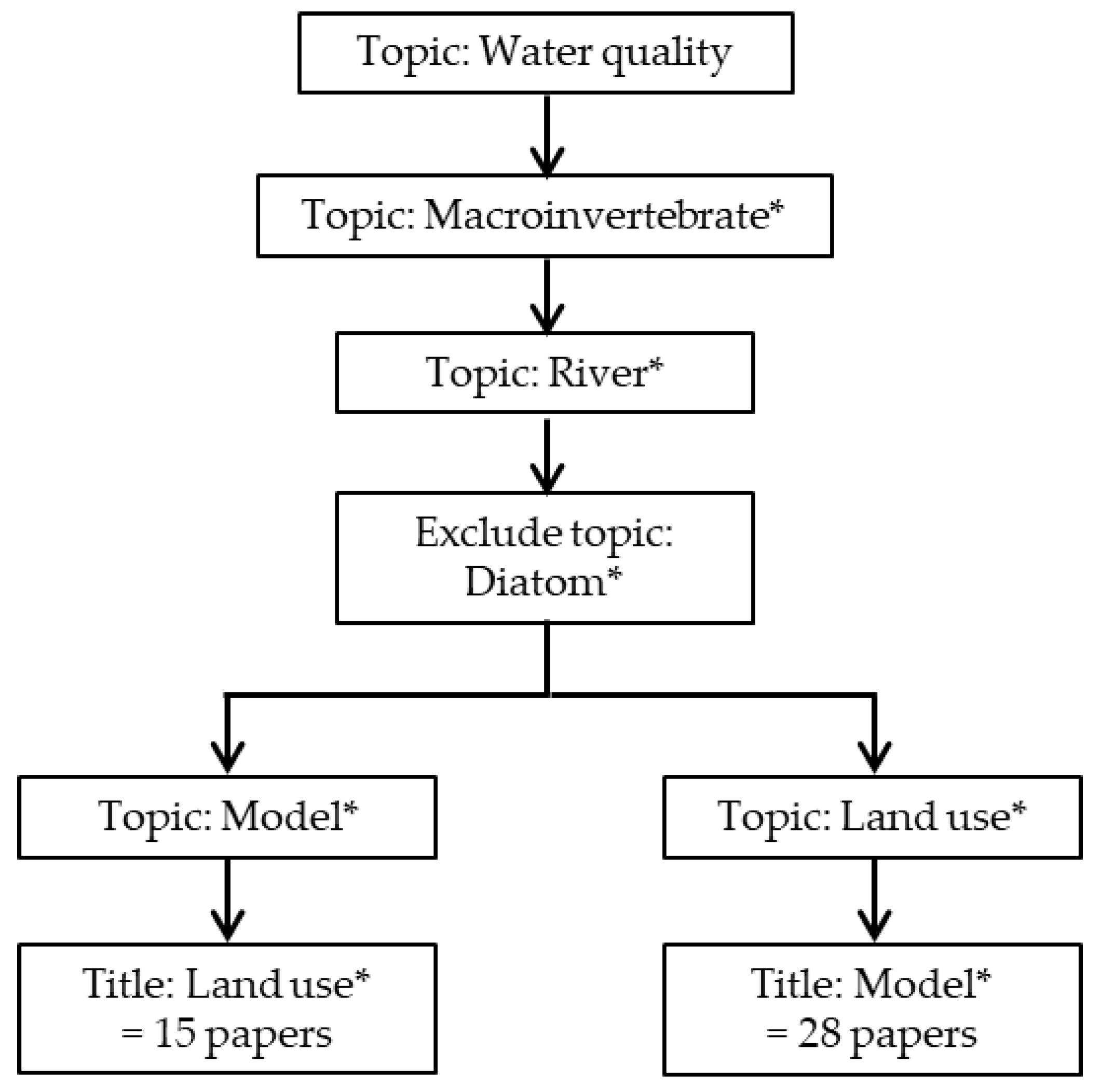
2. Materials and Methods
3. Ecological Water Quality Studies and Land Use
3.1. Introduction
3.2. Local or Riparian Land-Use Scale
3.3. Catchment or Regional Land-Use Scale
3.4. Recommendation for Integrated Local or Riparian and Catchment or Regional Land-Use Scales
3.5. Land-Use Change
4. Use of Models in Ecological Water Quality Studies
4.1. Input Variables
4.2. Ecological Models
4.3. Recommendation for Statistical Analysis and Model Selection
4.4. Strengths, Weaknesses, Opportunities, and Threats (SWOT) Analysis
5. Conclusions
Acknowledgments
Author Contributions
Conflicts of Interest
Appendix

| Impacts | Activities | |||||
|---|---|---|---|---|---|---|
| Agriculture | Urban | Forestry | Hydropower Generation and Water Storage | Mining | Industries | |
| Sedimentation | √ | √ | √ | √ | √ | √ |
| Eutrophication | √ | √ | √ | √ | √ | √ |
| Thermal pollution | √ | √ | √ | √ | √ | √ |
| Dissolved oxygen | √ | √ | √ | √ | ||
| Acidification | √ | √ | ||||
| Microbial contamination | √ | √ | ||||
| Salinization | √ | √ | √ | |||
| Metal pollution | √ | √ | √ | √ | √ | |
| Bio toxins | √ | √ | ||||
| Organic compounds | √ | √ | √ | √ | ||
| Micronutrient depletion | √ | |||||
| Country | Spatial Scale | Temporal | Scenario | |||
|---|---|---|---|---|---|---|
| Developed | Developing | Local or Riparian | Catchment/Regional | Combined | ||
| 31 | 8 | 21 | 7 | 11 | 2 | 5 |
| Remote Sensing | Field Observation | GIS | National Database | National Data + Satellite/GIS | National Data + Field Observation | Field Observation + Satellite/GIS | Satellite + GIS |
|---|---|---|---|---|---|---|---|
| 10 | 5 | 9 | 6 | 4 | 2 | 2 | 1 |
References
- Pilgrim, C.M.; Mikhailova, E.A.; Post, C.J.; Hains, J.J. Spatial and temporal analysis of land cover changes and water quality in the Lake Issaqueena watershed, South Carolina. Environ. Monit. Assess. 2014, 186, 7617–7630. [Google Scholar] [CrossRef] [PubMed]
- Garnier, J.; Brion, N.; Callens, J.; Passy, P.; Deligne, C.; Billen, G.; Servais, P.; Billen, C. Modeling historical changes in nutrient delivery and water quality of the Zenne River (1790s–2010): The role of land use, waterscape and urban wastewater management. J. Mar. Syst. 2013, 128, 62–76. [Google Scholar] [CrossRef]
- Da Silva, M.V.D.; Rosa, B.F.J.V.; Alves, R.G. Effect of mesohabitats on responses of invertebrate community structure in streams under different land uses. Environ. Monit. Assess. 2015, 187, 714. [Google Scholar] [CrossRef] [PubMed]
- Goss, C.W.; Goebel, P.C.; Sullivan, S.M.P. Shifts in attributes along agriculture-forest transitions of two streams in central Ohio, USA. Agric. Ecosyst. Environ. 2014, 197, 106–117. [Google Scholar] [CrossRef]
- Beasley, G.; Kneale, P. Reviewing the impact of metals and PAHs on macro invertebrates in urban watercourses. Prog. Phys. Geogr. 2002, 26, 236–270. [Google Scholar] [CrossRef]
- Smucker, N.J.; Detenbeck, N.E. Meta-Analysis of Lost Ecosystem Attributes in Urban Streams and the Effectiveness of Out-of-Channel Management Practices. Restor. Ecol. 2014, 22, 741–748. [Google Scholar] [CrossRef]
- Colin, N.; Maceda-Veiga, A.; Flor-Arnau, N.; Mora, J.; Fortuno, P.; Vieira, C.; Prat, N.; Cambra, J.; de Sostoa, A. Ecological impact and recovery of a Mediterranean river after receiving the effluent from a textile dyeing industry. Ecotoxicol. Environ. Saf. 2016, 132, 295–303. [Google Scholar] [CrossRef] [PubMed]
- Raper, E.; Davies, S.; Perkins, B.; Lamb, H.; Hermanson, M.; Soares, A.; Stephenson, T. Ecological conditions of ponds situated on blast furnace slag deposits located in South Gare Site of Special Scientific Interest (SSSI), Teesside, UK. Environ. Geochem. Health 2015, 37, 545–556. [Google Scholar] [CrossRef] [PubMed]
- Walsh, C.J.; Leonard, A.W.; Ladson, A.R.; Fletcher, T.D. Urban Stormwater and the Ecology of Streams; Cooperative Research Centre for Freshwater Ecology and Cooperative Research Centre for Catchment Hydrology: Canberra, Australia, 2004; ISBN 0-9751642-03. [Google Scholar]
- Kehoe, L.; Kuemmerle, T.; Meyer, C.; Levers, C.; Vaclavik, T.; Kreft, H. Global patterns of agricultural land-use intensity and vertebrate diversity. Divers. Distrib. 2015, 21, 1308–1318. [Google Scholar] [CrossRef]
- Roth, G.W. Crop Rotations and Conservation Tillage; College of Agricultural Sciences, The Pennsylvania State University: Pennsylvania, USA, 2017. [Google Scholar]
- Yates, A.G.; Bailey, R.C.; Schwindt, J.A. No-till cultivation improves stream ecosystem quality. J. Soil Water Conserv. 2006, 61, 14–19. [Google Scholar]
- Cortes, R.M.V.; Hughes, S.J.; Pereira, V.R.; Varandas, S.D.P. Tools for bioindicator assessment in rivers: The importance of spatial scale, land use patterns and biotic integration. Ecol. Indic. 2013, 34, 460–477. [Google Scholar] [CrossRef]
- Manfrin, A.; Bombi, P.; Traversetti, L.; Larsen, S.; Scalici, M. A landscape-based predictive approach for running water quality assessment: A Mediterranean case study. J. Nat. Conserv. 2016, 30, 27–31. [Google Scholar] [CrossRef]
- Thornhill, I.; Batty, L.; Death, R.G.; Friberg, N.R.; Ledger, M.E. Local and landscape scale determinants of macroinvertebrate assemblages and their conservation value in ponds across an urban land-use gradient. Biodivers. Conserv. 2017, 26, 1065–1086. [Google Scholar] [CrossRef]
- Pietron, J.; Chalov, S.R.; Chalova, A.S.; Alekseenko, A.V.; Jarsjo, J. Extreme spatial variability in riverine sediment load inputs due to soil loss in surface mining areas of the Lake Baikal basin. Catena 2017, 152, 82–93. [Google Scholar] [CrossRef]
- Alahuhta, J.; Virtala, A.; Hjort, J.; Ecke, F.; Johnson, L.B.; Sass, L.; Heino, J. Average niche breadths of species in lake macrophyte communities respond to ecological gradients variably in four regions on two continents. Oecologia 2017, 184, 219–235. [Google Scholar] [CrossRef] [PubMed]
- Hook, S.E.; Kroon, F.J.; Metcalfe, S.; Greenfield, P.A.; Moncuquet, P.; McGrath, A.; Smith, R.; Warne, M.S.J.; Turner, R.D.; McKeown, A.; et al. Global transcriptomic profiling in barramundi (Lates calcarifer) from rivers impacted by differing agricultural land uses. Environ. Toxicol. Chem. 2017, 36, 103–112. [Google Scholar] [CrossRef] [PubMed]
- Wright, R.F.; Couture, R.M.; Christiansen, A.B.; Guerrero, J.L.; Kaste, O.; Barlaup, B.T. Effects of multiple stresses hydropower, acid deposition and climate change on water chemistry and salmon populations in the River Otra, Norway. Sci. Total Environ. 2017, 574, 128–138. [Google Scholar] [CrossRef] [PubMed]
- Baillie, B.R.; Neary, D.G. Water quality in New Zealand’s planted forests: A review. N. Z. J. For. Sci. 2015, 45, 7. [Google Scholar] [CrossRef]
- Gerth, W.J.; Li, J.; Giannico, G.R. Agricultural land use and macroinvertebrate assemblages in lowland temporary streams of the Willamette Valley, Oregon, USA. Agric. Ecosyst. Environ. 2017, 236, 154–165. [Google Scholar] [CrossRef]
- Raapysjarvi, J.; Hamalainen, H.; Aroviita, J. Macrophytes in boreal streams: Characterizing and predicting native occurrence and abundance to assess human impact. Ecol. Indic. 2016, 64, 309–318. [Google Scholar] [CrossRef]
- Liu, H.; Bu, H.M.; Liu, G.H.; Wang, Z.X.; Liu, W.Z. Effects of surrounding land use on metal accumulation in environments and submerged plants in subtropical ponds. Environ. Sci. Pollut. Res. 2015, 22, 18750–18758. [Google Scholar] [CrossRef] [PubMed]
- Bonada, N.; Rieradevall, M.; Dallas, H.; Davis, J.; Day, J.; Figueroa, R.; Resh, V.H.; Prat, N. Multi-scale assessment of macroinvertebrate richness and composition in Mediterranean-climate rivers. Freshw. Biol. 2008, 53, 772–788. [Google Scholar] [CrossRef]
- Brown, L.R.; May, J.T.; Wulff, M. Associations of Benthic Macroinvertebrate Assemblages with Environmental Variables in the Upper Clear Creek Watershed, California. West. N. Am. Nat. 2012, 72, 473–494. [Google Scholar] [CrossRef]
- Yang, Y.Y.; Toor, G.S. Sources and mechanisms of nitrate and orthophosphate transport in urban stormwater runoff from residential catchments. Water Res. 2017, 112, 176–184. [Google Scholar] [CrossRef] [PubMed]
- Lee, F.; Simon, K.S.; Perry, G.L.W. Increasing agricultural land use is associated with the spread of an invasive fish (Gambusia affinis). Sci. Total Environ. 2017, 586, 1113–1123. [Google Scholar] [CrossRef] [PubMed]
- Brogna, D.; Michez, A.; Jacobs, S.; Dufrene, M.; Vincke, C.; Dendoncker, N. Linking Forest Cover to Water Quality: A Multivariate Analysis of Large Monitoring Datasets. Water 2017, 9, 176. [Google Scholar] [CrossRef]
- Cunha, E.J.; Montag, L.F.D.; Juen, L. Oil palm crops effects on environmental integrity of Amazonian streams and Heteropteran (Hemiptera) species diversity. Ecol. Indic. 2015, 52, 422–429. [Google Scholar] [CrossRef]
- Epele, L.B.; Miserendino, M.L. Environmental Quality and Aquatic Invertebrate Metrics Relationships at Patagonian Wetlands Subjected to Livestock Grazing Pressures. PLoS ONE 2015, 10, e0137873. [Google Scholar] [CrossRef] [PubMed]
- Sueyoshi, M.; Ishiyama, N.; Nakamura, F. beta-diversity decline of aquatic insects at the microhabitat scale associated with agricultural land use. Landsc. Ecol. Eng. 2016, 12, 187–196. [Google Scholar] [CrossRef]
- Palmer, M.A.; Menninger, H.L.; Bernhardt, E. River restoration, habitat heterogeneity and biodiversity: A failure of theory or practice? Freshw. Biol. 2010, 55, 205–222. [Google Scholar] [CrossRef]
- Palmer, M.A.; Hondula, K.L.; Koch, B.J. Ecological Restoration of Streams and Rivers: Shifting Strategies and Shifting Goals. Annu. Rev. Ecol. Evol. Syst. 2014, 45, 247–269. [Google Scholar] [CrossRef]
- Berger, E.; Haase, P.; Kuemmerlen, M.; Leps, M.; Schafer, R.B.; Sundermann, A. Water quality variables and pollution sources shaping stream macroinvertebrate communities. Sci. Total Environ. 2017, 587, 1–10. [Google Scholar] [CrossRef] [PubMed]
- Shrestha, M.K.; Recknagel, F.; Frizenschaf, J.; Meyer, W. Future climate and land uses effects on flow and nutrient loads of a Mediterranean catchment in South Australia. Sci. Total Environ. 2017, 590, 186–193. [Google Scholar] [CrossRef] [PubMed]
- Bussi, G.; Janes, V.; Whitehead, P.G.; Dadson, S.J.; Holman, I.P. Dynamic response of land use and river nutrient concentration to long-term climatic changes. Sci. Total Environ. 2017, 590, 818–831. [Google Scholar] [CrossRef] [PubMed]
- Fierro, P.; Bertran, C.; Mercado, M.; Pena-Cortes, F.; Tapia, J.; Hauenstein, E.; Caputo, L.; Vargas-Chacoff, L. Landscape composition as a determinant of diversity and functional feeding groups of aquatic macroinvertebrates in southern rivers of the Araucania, Chile. Lat. Am. J. Aquat. Res. 2015, 43, 186–200. [Google Scholar] [CrossRef]
- Jun, Y.C.; Kim, N.Y.; Kwon, S.J.; Han, S.C.; Hwang, I.C.; Park, J.H.; Won, D.H.; Byun, M.S.; Kong, H.Y.; Lee, J.E.; et al. Effects of land use on benthic macroinvertebrate communities: Comparison of two mountain streams in Korea. Ann. Limnol.-Int. J. Limnol. 2011, 47, S35–S49. [Google Scholar] [CrossRef]
- Park, S.R.; Lee, H.J.; Lee, S.W.; Hwang, S.J.; Byeon, M.S.; Joo, G.J.; Jeong, K.S.; Kong, D.S.; Kim, M.C. Relationships between land use and multi-dimensional characteristics of streams and rivers at two different scales. Ann. Limnol.-Int. J. Limnol. 2011, 47, S107–S116. [Google Scholar] [CrossRef]
- Hughes, S.J.; Cabral, J.A.; Bastos, R.; Cortes, R.; Vicente, J.; Eitelberg, D.; Yu, H.R.; Honrado, J.; Santos, M. A stochastic dynamic model to assess land use change scenarios on the ecological status of fluvial water bodies under the Water Framework Directive. Sci. Total Environ. 2016, 565, 427–439. [Google Scholar] [CrossRef] [PubMed]
- Schmalz, B.; Kuemmerlen, M.; Kiesel, J.; Cai, Q.; Jahnig, S.C.; Fohrer, N. Impacts of land use changes on hydrological components and macroinvertebrate distributions in the Poyang lake area. Ecohydrology 2015, 8, 1119–1136. [Google Scholar] [CrossRef]
- Tu, J. Combined impact of climate and land use changes on streamflow and water quality in eastern Massachusetts, USA. J. Hydrol. 2009, 379, 268–283. [Google Scholar] [CrossRef]
- McDonald, R.I.; Weber, K.F.; Padowski, J.; Boucher, T.; Shemie, D. Estimating watershed degradation over the last century and its impact on water-treatment costs for the world’s large cities. Proc. Natl. Acad. Sci. USA 2016, 113, 9117–9122. [Google Scholar] [CrossRef] [PubMed]
- Bucker, A.; Sondermann, M.; Frede, H.G.; Breuer, L. The influence of land-use on macroinvertebrate communities in montane tropical streams—A case study from Ecuador. Fundam. Appl. Limnol. 2010, 177, 267–282. [Google Scholar] [CrossRef]
- Mwedzi, T.; Bere, T.; Mangadze, T. Macroinvertebrate assemblages in agricultural, mining, and urban tropical streams: Implications for conservation and management. Environ. Sci. Pollut. Res. 2016, 23, 11181–11192. [Google Scholar] [CrossRef] [PubMed]
- Strehmel, A.; Schmalz, B.; Fohrer, N. Evaluation of Land Use, Land Management and Soil Conservation Strategies to Reduce Non-Point Source Pollution Loads in the Three Gorges Region, China. Environ. Manag. 2016, 58, 906–921. [Google Scholar] [CrossRef] [PubMed]
- Everaert, G.; Pauwels, I.S.; Boets, P.; Verduin, E.; de la Haye, M.A.A.; Blom, C.; Goethals, P.L.M. Model-based evaluation of ecological bank design and management in the scope of the European Water Framework Directive. Ecol. Eng. 2013, 53, 144–152. [Google Scholar] [CrossRef]
- Arias-Hidalgo, M.; Villa-Cox, G.; Griensven, A.V.; Solorzano, G.; Villa-Cox, R.; Mynett, A.E.; Debels, P. A decision framework for wetland management in a river basin context: The “Abras de Mantequilla” case study in the Guayas River Basin, Ecuador. Environ. Sci. Policy 2013, 34, 103–114. [Google Scholar] [CrossRef]
- Schuwirth, N.; Dietzel, A.; Reichert, P. The importance of biotic interactions for the prediction of macroinvertebrate communities under multiple stressors. Funct. Ecol. 2016, 30, 974–984. [Google Scholar] [CrossRef]
- Tchakonte, S.; Ajeagah, G.A.; Camara, A.I.; Diomande, D.; Tchatcho, N.L.N.; Ngassam, P. Impact of urbanization on aquatic insect assemblages in the coastal zone of Cameroon: The use of biotraits and indicator taxa to assess environmental pollution. Hydrobiologia 2015, 755, 123–144. [Google Scholar] [CrossRef]
- Slevers, M.; Hale, R.; Morrongiello, J.R. Do trout respond to riparian change? A meta-analysis with implications for restoration and management. Freshw. Biol. 2017, 62, 445–457. [Google Scholar] [CrossRef]
- Ferreira, A.R.L.; Fernandes, L.F.S.; Cortes, R.M.V.; Pacheco, F.A.L. Assessing anthropogenic impacts on riverine ecosystems using nested partial least squares regression. Sci. Total Environ. 2017, 583, 466–477. [Google Scholar] [CrossRef] [PubMed]
- Larras, F.; Coulaud, R.; Gautreau, E.; Billoir, E.; Rosebery, J.; Usseglio-Polatera, P. Assessing anthropogenic pressures on streams: A random forest approach based on benthic diatom communities. Sci. Total Environ. 2017, 586, 1101–1112. [Google Scholar] [CrossRef] [PubMed]
- Dahm, V.; Hering, D. A modeling approach for identifying recolonisation source sites in river restoration planning. Landsc. Ecol. 2016, 31, 2323–2342. [Google Scholar] [CrossRef]
- Pearson, C.E.; Ormerod, S.J.; Symondson, W.O.C.; Vaughan, I.P. Resolving large-scale pressures on species and ecosystems: Propensity modelling identifies agricultural effects on streams. J. Appl. Ecol. 2016, 53, 408–417. [Google Scholar] [CrossRef] [PubMed]
- Weigel, B.M. Development of stream macroinvertebrate models that predict watershed and local stressors in Wisconsin. J. N. Am. Benthol. Soc. 2003, 22, 123–142. [Google Scholar] [CrossRef]
- Abouali, M.; Nejadhashemi, A.P.; Daneshvar, F.; Woznicki, S.A. Two-phase approach to improve stream health modeling. Ecol. Inform. 2016, 34, 13–21. [Google Scholar] [CrossRef]
- Alemneh, T.; Ambelu, A.; Bahrndorff, S.; Mereta, S.T.; Pertoldi, C.; Zaitchik, B.F. Modeling the impact of highland settlements on ecological disturbance of streams in Choke Mountain Catchment: Macroinvertebrate assemblages and water quality. Ecol. Indic. 2017, 73, 452–459. [Google Scholar] [CrossRef]
- Alvarez-Cabria, M.; Gonzalez-Ferreras, A.M.; Penas, F.J.; Barquin, J. Modelling macroinvertebrate and fish biotic indices: From reaches to entire river networks. Sci. Total Environ. 2017, 577, 308–318. [Google Scholar] [CrossRef] [PubMed]
- Baltazar, D.E.S.; Magcale-Macandog, D.; Tan, M.F.O.; Zafaralla, M.T.; Cadiz, N.M. A River Health Status Model Based on Water Quality, Macroinvertebrates and Land Use for Niyugan River, Cabuyao City, Laguna, Philippines. J. Environ. Sci. Manag. 2016, 19, 38–53. [Google Scholar]
- Damanik-Ambarita, M.N.; Everaert, G.; Forio, M.A.E.; Nguyen, T.H.T.; Lock, K.; Musonge, P.L.S.; Suhareva, N.; Dominguez-Granda, L.; Bennetsen, E.; Boets, P.; et al. Generalized Linear Models to Identify Key Hydromorphological and Chemical Variables Determining the Occurrence of Macroinvertebrates in the Guayas River Basin (Ecuador). Water 2016, 8, 297. [Google Scholar] [CrossRef] [Green Version]
- Einheuser, M.D.; Nejadhashemi, A.P.; Sowa, S.P.; Wang, L.Z.; Hamaamin, Y.A.; Woznicki, S.A. Modeling the effects of conservation practices on stream health. Sci. Total Environ. 2012, 435, 380–391. [Google Scholar] [CrossRef] [PubMed]
- Erba, S.; Pace, G.; Demartini, D.; Di Pasquale, D.; Dorflinger, G.; Buffagni, A. Land use at the reach scale as a major determinant for benthic invertebrate community in Mediterranean rivers of Cyprus. Ecol. Indic. 2015, 48, 477–491. [Google Scholar] [CrossRef]
- Forio, M.A.E.; Landuyt, D.; Bennetsen, E.; Lock, K.; Nguyen, T.H.T.; Damanik-Ambarita, M.N.; Musonge, P.L.S.; Boets, P.; Everaert, G.; Dominguez-Granda, L.; et al. Bayesian belief network models to analyse and predict ecological water quality in rivers. Ecol. Model. 2015, 312, 222–238. [Google Scholar] [CrossRef]
- Forio, M.A.E.; Mouton, A.; Lock, K.; Boets, P.; Tien, N.T.H.; Damanik-Ambarita, M.N.; Musonge, P.L.S.; Dominguez-Granda, L.; Goethals, P.L.M. Fuzzy modelling to identify key drivers of ecological water quality to support decision and policy making. Environ. Sci. Policy 2017, 67, 58–68. [Google Scholar] [CrossRef]
- Hrodey, P.J.; Sutton, T.M.; Frimpong, E.A.; Simon, T.P. Land-use Impacts on Watershed Health and Integrity in Indiana Warmwater Streams. Am. Midl. Nat. 2009, 161, 76–95. [Google Scholar] [CrossRef]
- Mantyka-Pringle, C.S.; Martin, T.G.; Moffatt, D.B.; Linke, S.; Rhodes, J.R. Understanding and predicting the combined effects of climate change and land-use change on freshwater macroinvertebrates and fish. J. Appl. Ecol. 2014, 51, 572–581. [Google Scholar] [CrossRef]
- Moreno, P.; Franca, J.S.; Ferreira, W.R.; Paz, A.D.; Monteiro, I.M.; Callisto, M. Use of the BEAST model for biomonitoring water quality in a neotropical basin. Hydrobiologia 2009, 630, 231–242. [Google Scholar] [CrossRef]
- Sanchez, G.M.; Nejadhashemi, A.P.; Zhang, Z.; Woznicki, S.A.; Habron, G.; Marquart-Pyatt, S.; Shortridge, A. Development of a socio-ecological environmental justice model for watershed-based management. J. Hydrol. 2014, 518, 162–177. [Google Scholar] [CrossRef]
- Sheldon, F.; Peterson, E.E.; Boone, E.L.; Sippel, S.; Bunn, S.E.; Harch, B.D. Identifying the spatial scale of land use that most strongly influences overall river ecosystem health score. Ecol. Appl. 2012, 22, 2188–2203. [Google Scholar] [CrossRef] [PubMed]
- Woznicki, S.A.; Nejadhashemi, A.P.; Abouali, M.; Herman, M.R.; Esfahanian, E.; Hamaamin, Y.A.; Zhang, Z. Ecohydrological modeling for large-scale environmental impact assessment. Sci. Total Environ. 2016, 543, 274–286. [Google Scholar] [CrossRef] [PubMed]
- Zhang, Y.X.; Dudgeon, D.; Cheng, D.S.; Thoe, W.; Fok, L.; Wang, Z.Y.; Lee, J.H.W. Impacts of land use and water quality on macroinvertebrate communities in the Pearl River drainage basin, China. Hydrobiologia 2010, 652, 71–88. [Google Scholar] [CrossRef]
- Barton, D.R. The use of Percent Model Affinity to assess the effects of agriculture on benthic invertebrate communities in headwater streams of southern Ontario, Canada. Freshw. Biol. 1996, 36, 397–410. [Google Scholar] [CrossRef]
- Bennetsen, E.; Gobeyn, S.; Goethals, P.L.M. Species distribution models grounded in ecological theory for decision support in river management. Ecol. Model. 2016, 325, 1–12. [Google Scholar] [CrossRef]
- Carlisle, D.M.; Hawkins, C.P. Land use and the structure of western US stream invertebrate assemblages: Predictive models and ecological traits. J. N. Am. Benthol. Soc. 2008, 27, 986–999. [Google Scholar] [CrossRef]
- Carlisle, D.M.; Meador, M.R. A biological assessment of streams in the eastern united states using a predictive model for macroinvertebrate assemblages. J. Am. Water Resour. Assoc. 2007, 43, 1194–1207. [Google Scholar] [CrossRef]
- Clapcott, J.E.; Goodwin, E.O.; Snelder, T.H.; Collier, K.J.; Neale, M.W.; Greenfield, S. Finding reference: A comparison of modelling approaches for predicting macroinvertebrate community index benchmarks. N. Z. J. Mar. Freshw. Res. 2017, 51, 44–59. [Google Scholar] [CrossRef]
- Davies, S.P.; Jackson, S.K. The biological condition gradient: A descriptive model for interpreting change in aquatic ecosystems. Ecol. Appl. 2006, 16, 1251–1266. [Google Scholar] [CrossRef]
- Feio, M.J.; Norris, R.H.; Graca, M.A.S.; Nichols, S. Water quality assessment of Portuguese streams: Regional or national predictive models? Ecol. Indic. 2009, 9, 791–806. [Google Scholar] [CrossRef]
- Feio, M.J.; Reynoldson, T.B.; Ferreira, V.; Graca, M.A.S. A predictive model for freshwater bioassessment (Mondego River, Portugal). Hydrobiologia 2007, 589, 55–68. [Google Scholar] [CrossRef]
- Guse, B.; Kail, J.; Radinger, J.; Schroder, M.; Kiesel, J.; Hering, D.; Wolter, C.; Fohrer, N. Eco-hydrologic model cascades: Simulating land use and climate change impacts on hydrology, hydraulics and habitats for fish and macroinvertebrates. Sci. Total Environ. 2015, 533, 542–556. [Google Scholar] [CrossRef] [PubMed]
- Hawkins, C.P.; Norris, R.H.; Hogue, J.N.; Feminella, J.W. Development and evaluation of predictive models for measuring the biological integrity of streams. Ecol. Appl. 2000, 10, 1456–1477. [Google Scholar] [CrossRef]
- Hawkins, C.P.; Yuan, L.L. Multitaxon distribution models reveal severe alteration in the regional biodiversity of freshwater invertebrates. Freshw. Sci. 2016, 35, 1365–1376. [Google Scholar] [CrossRef]
- Maloney, K.O.; Weller, D.E. Anthropogenic disturbance and streams: Land use and land-use change affect stream ecosystems via multiple pathways. Freshw. Biol. 2011, 56, 611–626. [Google Scholar] [CrossRef]
- Terrado, M.; Sabater, S.; Chaplin-Kramer, B.; Mandle, L.; Ziv, G.; Acuna, V. Model development for the assessment of terrestrial and aquatic habitat quality in conservation planning. Sci. Total Environ. 2016, 540, 63–70. [Google Scholar] [CrossRef] [PubMed]
- Lock, K.; Goethals, P.L.M. Habitat suitability modelling for mayflies (Ephemeroptera) in Flanders (Belgium). Ecol. Inform. 2013, 17, 30–35. [Google Scholar] [CrossRef]
- Lock, K.; Goethals, P.L.M. Predicting the occurrence of stoneflies (Plecoptera) on the basis of water characteristics, river morphology and land use. J. Hydroinform. 2014, 16, 812–821. [Google Scholar] [CrossRef]
- Van Sickle, J.; Baker, J.; Herlihy, A.; Bayley, P.; Gregory, S.; Haggerty, P.; Ashkenas, L.; Li, J. Projecting the biological condition of streams under alternative scenarios of human land use. Ecol. Appl. 2004, 14, 368–380. [Google Scholar] [CrossRef]
- Carr, G.M.; Neary, J.P. Water Quality for Ecosystem and Human Health, 2nd ed.; Robarts, R., Barker, S., Eds.; United Nations Environment Programme (UNEP); Global Environment Monitoring System (GEMS)/Water Programme: Burlington, ON, Canada, 2008; p. 120. ISBN 92-95039-51-7. [Google Scholar]
- Kuemmerle, T.; Erb, K.; Meyfroidt, P.; Muller, D.; Verburg, P.H.; Estel, S.; Haberl, H.; Hostert, P.; Jepsen, M.R.; Kastner, T.; et al. Challenges and opportunities in mapping land use intensity gIobally. Curr. Opin. Environ. Sustain. 2013, 5, 484–493. [Google Scholar] [CrossRef] [PubMed]
- Crétaz, A.L.D.L.; Barten, P.K. Land Use Effects on Streamflow and Water Quality in the Northeastern United States; CRC: Boca Raton, FL, USA, 2007; p. 319. ISBN 9780849391873, 0849391873. [Google Scholar]
- Rios-Touma, B.; Prescott, C.; Axtell, S.; Kondolf, G.M. Habitat Restoration in the Context of Watershed Prioritization: The Ecological Performance of Urban Stream Restoration Projects in Portland, Oregon. River Res. Appl. 2015, 31, 755–766. [Google Scholar] [CrossRef]
- Waite, I.R. Agricultural disturbance response models for invertebrate and algal metrics from streams at two spatial scales within the U.S. Hydrobiologia 2014, 726, 285–303. [Google Scholar] [CrossRef]
- Molina, M.C.; Roa-Fuentes, C.A.; Zeni, J.O.; Casatti, L. The effects of land use at different spatial scales on instream features in agricultural streams. Limnologica 2017, 65, 14–21. [Google Scholar] [CrossRef]
- Usio, N.; Nakagawa, M.; Aoki, T.; Higuchi, S.; Kadono, Y.; Akasaka, M.; Takamura, N. Effects of land use on trophic states and multi-taxonomic diversity in Japanese farm ponds. Agric. Ecosyst. Environ. 2017, 247, 205–215. [Google Scholar] [CrossRef]
- Lee, B.Y.; Park, S.J.; Paule, M.C.; Jun, W.; Lee, C.H. Effects of Impervious Cover on the Surface Water Quality and Aquatic Ecosystem of the Kyeongan Stream in South Korea. Water Environ. Res. 2012, 84, 635–645. [Google Scholar] [CrossRef] [PubMed]
- Wen, T.; Sheng, S.; An, S.Q. Relationships between stream ecosystem properties and landscape composition at multiple spatial scales along a heavily polluted stream in China: Implications for restoration. Ecol. Eng. 2016, 97, 493–502. [Google Scholar] [CrossRef]
- De Morais, L.; de Oliveira Sanches, B.; Sanches, B.D.O.; Kaufmann, P.R.; Hughes, R.M.; Molozzi, J.; Callisto, M. Assessment of disturbance at three spatial scales in two large tropical reservoirs. J. Limnol. 2017, 76, 240–252. [Google Scholar] [CrossRef]
- Raymond, K.L.; Vondracek, B. Relationships among rotational and conventional grazing systems, stream channels, and macroinvertebrates. Hydrobiologia 2011, 669, 105–117. [Google Scholar] [CrossRef]
- Jayawardana, J.M.C.K.; Gunawardana, W.D.T.M.; Udayakumara, E.P.N.; Westbrooke, M. Land use impacts on river health of Uma Oya, Sri Lanka: Implications of spatial scales. Environ. Monit. Assess. 2017, 189. [Google Scholar] [CrossRef] [PubMed]
- Merriam, E.R.; Petty, J.T.; Merovich, G.T.; Fulton, J.B.; Strager, M.P. Additive effects of mining and residential development on stream conditions in a central Appalachian watershed. J. N. Am. Benthol. Soc. 2011, 30, 399–418. [Google Scholar] [CrossRef]
- Meyer, M.D.; Davis, C.A.; Dvorett, D. Response of Wetland Invertebrate Communities to Local and Landscape Factors in North Central Oklahoma. Wetlands 2015, 35, 533–546. [Google Scholar] [CrossRef]
- Carvalho, L.; Cortes, R.; Bordalo, A.A. Evaluation of the ecological status of an impaired watershed by using a multi-index approach. Environ. Monit. Assess. 2011, 174, 493–508. [Google Scholar] [CrossRef] [PubMed]
- Bellucci, C.J.; Becker, M.; Beauchene, M. Characteristics of Macroinvertebrate and Fish Communities From 30 Least Disturbed Small Streams in Connecticut. Northeast. Nat. 2011, 18, 411–444. [Google Scholar] [CrossRef]
- Lowrance, R.; Altier, L.S.; Newbold, J.D.; Schnabel, R.R.; Groffman, P.M.; Denver, J.M.; Correll, D.L.; Gilliam, J.W.; Robinson, J.L.; Brinsfield, R.B.; et al. Water quality functions of riparian forest buffers in Chesapeake Bay watersheds. Environ. Manag. 1997, 21, 687–712. [Google Scholar] [CrossRef]
- Rocchini, D.; Petras, V.; Petrasova, A.; Horning, N.; Furtkevicova, L.; Neteler, M.; Leutner, B.; Wegmann, M. Open data and open source for remote sensing training in ecology. Ecol. Inform. 2017, 40, 57–61. [Google Scholar] [CrossRef]
- Harding, J.S.; Benfield, E.F.; Bolstad, P.V.; Helfman, G.S.; Jones, E.B.D. Stream biodiversity: The ghost of land use past. Proc. Natl. Acad. Sci. USA 1998, 95, 14843–14847. [Google Scholar] [CrossRef] [PubMed]
- Verkaik, I.; Vila-Escale, M.; Rieradevall, M.; Baxter, C.V.; Lake, P.S.; Minshall, G.W.; Reich, P.; Prat, N. Stream macroinvertebrate community responses to fire: Are they the same in different fire-prone biogeographic regions? Freshw. Sci. 2015, 34, 1527–1541. [Google Scholar] [CrossRef]
- Strauch, A.M.; MacKenzie, R.A.; Giardina, C.P.; Bruland, G.L. Climate driven changes to rainfall and streamflow patterns in a model tropical island hydrological system. J. Hydrol. 2015, 523, 160–169. [Google Scholar] [CrossRef]
- Barber, L.B.; Paschke, S.S.; Battaglia, W.A.; Douville, C.; Fitzgerald, K.C.; Keefe, S.H.; Roth, D.A.; Vajda, A.M. Effects of an Extreme Flood on Trace Elements in River Water-From Urban Stream to Major River Basin. Environ. Sci. Technol. 2017, 51, 10344–10356. [Google Scholar] [CrossRef] [PubMed]
- Milliman, J.D.; Lee, T.Y.; Huang, J.C.; Kao, S.J. Impact of catastrophic events on small mountainous rivers: Temporal and spatial variations in suspendedand dissolved-solid fluxes along the Choshui River, central western Taiwan, during typhoon Mindulle, 2–6 July 2004. Geochim. Cosmochim. Acta 2017, 205, 272–294. [Google Scholar] [CrossRef]
- Lofgren, S.; Grandin, U.; Stendera, S. Long-term effects on nitrogen and benthic fauna of extreme weather events: Examples from two Swedish headwater streams. Ambio 2014, 43, 58–76. [Google Scholar] [CrossRef] [PubMed]
- Bixby, R.J.; Cooper, S.D.; Gresswell, R.E.; Brown, L.E.; Dahm, C.N.; Dwire, K.A. Fire effects on aquatic ecosystems: An assessment of the current state of the science. Freshw. Sci. 2015, 34, 1340–1350. [Google Scholar] [CrossRef]
- Rocchini, D.; Petras, V.; Petrasova, A.; Chemin, Y.; Ricotta, C.; Frigeri, A.; Landa, M.; Marcantonio, M.; Bastin, L.; Metz, M.; et al. Spatio-ecological complexity measures in GRASS GIS. Comput. Geosci. 2017, 104, 166–176. [Google Scholar] [CrossRef]
- Greenacre, M.; Primicerio, R. Multivariate Analysis of Ecological Data; Fundación BBVA: Bilbao, Spain, 2013; ISBN 978-84-92937-50-9. [Google Scholar]
- Crawley, M.J. The R Book; Wiley: Chichester, UK, 2007; Volume viii, p. 942. ISBN 9780470510247, 0470510242. [Google Scholar]
- Zuur, A.F.; Ieno, E.N.; Smith, G.M. Analysing Ecological Data; Statistics for biology and health; Springer: New York, NY, USA, 2007; Volume xxvi, p. 672. ISBN 9780387459677 (hbk.). [Google Scholar]
- Paliy, O.; Shankar, V. Application of multivariate statistical techniques in microbial ecology. Mol. Ecol. 2016, 25, 1032–1057. [Google Scholar] [CrossRef] [PubMed]
- Dalgaard, P. Introductory Statistics with R, 2nd ed.; Statistics and computing; Springer: New York, NY, USA, 2008; Volume xvi, p. 363. ISBN 9780387790534 (pbk. alk. paper), 0387790535 (pbk. alk. paper) 1431-8784. [Google Scholar]
- Tuffery, S. Data Mining and Statistics for Decision Making; Wiley series in computational statistics; Wiley: Chichester, UK; Hoboken, NJ, USA, 2011; Volume xxiv, p. 689. ISBN 9780470688298 (hardback). [Google Scholar]
- Berk, R.A. Statistical Learning from a Regression Perspective; Springer series in statistics; Springer Verlag: New York, NY, USA, 2008; Volume xvii, p. 358. ISBN 9780387775005, 0387775005. [Google Scholar]
- Van Echelpoel, W.; Boets, P.; Landuyt, D.; Gobeyn, S.; Everaert, G.; Bennetsen, E.; Mouton, A.; Goethals, P.L.M. Species distribution models for sustainable ecosystem management. Adv. Model. Tech. Stud. Glob. Chang. Environ. Sci. 2015, 27, 115–134. [Google Scholar] [CrossRef]
- Zuur, A.F.; Ieno, E.N.; Elphick, C.S. A protocol for data exploration to avoid common statistical problems. Methods Ecol. Evol. 2010, 1, 3–14. [Google Scholar] [CrossRef]
- Witten, I.H.; Frank, E. Data Mining: Practical Machine Learning Tools and Techniques, 2nd ed.; Morgan Kaufmann series in data management systems; Morgan Kaufman: Amsterdam, The Netherlands; Boston, MA, USA, 2005; Volume xxxi, p. 525. ISBN 0120884070. [Google Scholar]
- Shmueli, G. To Explain or to Predict? Stat. Sci. 2010, 25, 289–310. [Google Scholar] [CrossRef]
- Zuur, A.F. Mixed Effects Models and Extensions in Ecology with R; Statistics for biology and health; Springer: New York, NY, USA, 2009; Volume xxii, p. 574. ISBN 9780387874579 (hbk.), 0387874577 (hbk.). [Google Scholar]
- Damanik-Ambarita, M.N.; Lock, K.; Boets, P.; Everaert, G.; Nguyen, T.H.T.; Forio, M.A.E.; Musonge, P.L.S.; Suhareva, N.; Bennetsen, E.; Landuyt, D.; et al. Ecological water quality analysis of the Guayas river basin (Ecuador) based on macroinvertebrates indices. Limnologica 2016. [Google Scholar] [CrossRef]
- Cereghino, R.; Giraudel, J.L.; Compin, A. Spatial analysis of stream invertebrates distribution in the Adour-Garonne drainage basin (France), using Kohonen self organizing maps. Ecol. Model. 2001, 146, 167–180. [Google Scholar] [CrossRef]
- Goethals, P.L.M.; Dedecker, A.P.; Gabriels, W.; Lek, S.; De Pauw, N. Applications of artificial neural networks predicting macroinvertebrates in freshwaters. Aquat. Ecol. 2007, 41, 491–508. [Google Scholar] [CrossRef]
- Yang, L.; Bai, X.; Hu, Y. Comparison between the linear model and k-nearest neighbor method for predicting macroinvertebrate assemblages in a city river in Beijing, China. Appl. Ecol. Environ. Res. 2017, 16, 387–406. [Google Scholar] [CrossRef]
- Nirmalakhandan, N. Modeling Tools for Environmental Engineers and Scientists; CRC Press: Boca Raton, FL, USA, 2002; Volume xi, p. 312. ISBN 1566769957. [Google Scholar]
- Paillex, A.; Reichert, P.; Lorenz, A.W.; Schuwirth, N. Mechanistic modelling for predicting the effects of restoration, invasion and pollution on benthic macroinvertebrate communities in rivers. Freshw. Biol. 2017, 62, 1083–1093. [Google Scholar] [CrossRef]
- Guisan, A.; Zimmermann, N.E. Predictive habitat distribution models in ecology. Ecol. Model. 2000, 135, 147–186. [Google Scholar] [CrossRef]
- Alvarez-Mieles, G.; Irvine, K.; Griensven, A.V.; Arias-Hidalgo, M.; Torres, A.; Mynett, A.E. Relationships between aquatic biotic communities and water quality in a tropical river-wetland system (Ecuador). Environ. Sci. Policy 2013, 34, 115–127. [Google Scholar] [CrossRef]
- R-Core-Team. R: A Language and Environment for Statistical Computing; R Foundation for Statistical Computing: Vienna, Austria, 2013. [Google Scholar]
- Hubbart, J.A.; Kellner, E.; Kinder, P.; Stephan, K. Challenges in aquatic physical habitat assessment: Improving conservation and restoration decisions for contemporary watersheds. Challenges 2017, 8, 11. [Google Scholar] [CrossRef]

| Identification Level | Data Source | Biotic Index | ||||||
|---|---|---|---|---|---|---|---|---|
| Family Level | Mostly Species or Genus Level, Some Up to Family Level | Order Level | No Information | Sampling (Kick, Surber) | National/Regional Databases | No Biotic index, Only Taxa Richness | Biotic Index (e.g., Hilsenhoff, EPT, BMWP, ASPT) | Diversity Indices (Simpson’s Diversity, Shannon–Wiener Index) |
| Abouali et al. [57], Alemneh et al. [58], Alvarez-Cabria et al. [59], Baltazar et al. [60], Cortes et al. [13], [61], Einheuser et al. [62], Erba et al. [63], Forio et al. [64], Forio et al. [65], Hrodey et al. [66], Hughes et al. [40], Mantyka-Pringle et al. [67], Moreno et al. [68], Pearson et al. [55], Sanchez et al. [69], Sheldon et al. [70], Woznicki et al. [71], Zhang et al. [72] | Barton [73], Bennetsen et al. [74], Carlisle and Hawkins [75], Carlisle and Meador [76], Clapcott et al. [77], Dahm and Hering [54], Davies and Jackson [78], Feio et al. [79], Feio et al. [80], Guse et al. [81], Hawkins et al. [82], Hawkins and Yuan [83], Maloney and Weller [84], Schmalz et al. [41], Sueyoshi et al. [31], Terrado et al. [85], Weigel [56] | Lock and Goethals [86], Lock and Goethals [87] | Van Sickle et al. [88] | Alemneh et al. [58] kick, Baltazar et al. [60] kick, Barton [73] kick, Cortes et al. [13], Damanik-Ambarita et al. [61] kick, Erba et al. [63] surber, Feio et al. [80] kick, Forio et al. [64] kick, Forio et al. [65] kick, Hawkins et al. [82] surber, Hrodey et al. [66] Ekman dredge + kick + surber, Lock and Goethals [86] kick, Lock and Goethals [87] kick, Maloney and Weller [84] kick, Moreno et al. [68] surber, Pearson et al. [55] kick, Schmalz et al. [41], Sueyoshi et al. [31] surber, Zhang et al. [72] kick | Abouali et al. [57], Alvarez-Cabria et al. [59] kick, Bennetsen et al. [74], Carlisle and Hawkins [75] slack, Carlisle and Meador [76] slack, Clapcott et al. [77] kick + surber, Dahm and Hering [54], Davies and Jackson [78], Einheuser et al. [62], Feio et al. [79] kick, Guse et al. [81], Hawkins and Yuan [83], Hughes et al. [40], Mantyka-Pringle et al. [67], Sanchez et al. [69], Sheldon et al. [70], Terrado et al. [85], Van Sickle et al. [88], Weigel [56], Woznicki et al. [71] | Alemneh et al. [58], Bennetsen et al. [74], Carlisle and Hawkins [75], Carlisle and Meador [76], Dahm and Hering [54], Davies and Jackson [78], Feio et al. [79], Feio et al. [80], Guse et al. [81], Hawkins et al. [82], Hawkins and Yuan [83], Lock and Goethals [86], Lock and Goethals [87], Mantyka-Pringle et al. [67], Schmalz et al. [41], Sueyoshi et al. [31], | Abouali et al. [57], Alvarez-Cabria et al. [59], Baltazar et al. [60], Barton [73], Clapcott et al. [77], Cortes et al. [13], Damanik-Ambarita et al. [61], Einheuser et al. [62], Erba et al. [63], Forio et al. [64], Forio et al. [65], Hrodey et al. [66], Hughes et al. [40], Maloney and Weller [84], Pearson et al. [55], Sanchez et al. [69], Sheldon et al. [70], Van Sickle et al. [88], Weigel [56], Woznicki et al. [71], Zhang et al. [72] | Baltazar et al. [60], Erba et al. [63], Moreno et al. [68], Pearson et al. [55], Terrado et al. [85], Weigel [56] |
| Used Land-Use Information | Land-Use Effects | ||
|---|---|---|---|
| Positive | Negative | Not Defined or Not Studied | |
| Urban, industrial | Alemneh et al. [58], Baltazar et al. [60], Carlisle and Meador [76], Cortes et al. [13], Lock and Goethals [87], Lock and Goethals [86], Sanchez et al. [69] | ||
| Agricultural (arable, pasture, orchard, etc.) | Barton [73], Hrodey et al. [66], Pearson et al. [55], Sueyoshi et al. [31], Weigel [56] | ||
| Forest | Sheldon et al. [70] | ||
| Agricultural + urban | Maloney and Weller [84], Van Sickle et al. [88], Zhang et al. [72] | ||
| Land use is divided into clear classes | Abouali et al. [57], Alvarez-Cabria et al. [59], Clapcott et al. [77], Dahm and Hering [54], Damanik-Ambarita et al. [61], Erba et al. [63], Feio et al. [79], Feio et al. [80], Forio et al. [64], Forio et al. [65], Hawkins et al. [82], Mantyka-Pringle et al. [67], Woznicki et al. [71] | ||
| Land use classification is not provided | Bennetsen et al. [74], Davies and Jackson [78], Hawkins and Yuan [83], Moreno et al. [68] | ||
| Scenario best management practices | Einheuser et al. [62], Hughes et al. [40], Schmalz et al. [41], Terrado et al. [85] | ||
| Scenario crop rotations | Guse et al. [81] | ||
| Mixed use (combination of agricultural, residential, forest, etc.) | Carlisle and Hawkins [75] | ||
| Local or Riparian Scale (m) | Authors | Catchment Scale (km2) | Authors |
|---|---|---|---|
| 30 | Abouali et al. [57], Hrodey et al. [66] | 17 | Rios-Touma et al. [92] |
| 1000 radius | Cortes et al. [13], Feio et al. [80] | 6378 | Waite [93] |
| 150 radius | Molina et al. [94] | 33 | Molina et al. [94] |
| 10, 100, 250, 500, 1000, 2000 | Usio et al. [95] | 447 | Lee et al. [96] |
| 50, 100, 250, 500, 1000, 2500 | Thornhill et al. [15] | 5896 | Wen et al. [97] |
| 250 radius | de Morais et al. [98] | 181 | Raymond and Vondracek [99] |
| 200 × 300 | Jayawardana et al. [100] | 765 | Jayawardana et al. [100] |
| 500-, 1000-, 2500-, 5000 × 100 | Dahm and Hering [54] | 173 | Merriam et al. [101] |
| 100, 1000 | Meyer et al. [102] | 35 | Carvalho et al. [103] |
| 500 length or radius | Erba et al. [63], Pearson et al. [55], Mantyka-Pringle et al. [67] | 2000 | Bellucci et al. [104] |
| 30, 120 width | Van Sickle et al. [88] | 9162 | Park et al. [39] |
| Type of Variables | # of Studies | References |
|---|---|---|
| Geomorphology (e.g., elevation, river banks, and sediment type) | 1 | Barton [73] |
| Hydrology (e.g., annual discharge and flow) + physico-chemical (e.g., nutrients and pH) | 1 | Sanchez et al. [69] |
| Geomorphology + meteorology (e.g., rainfall and snow fall) | 1 | Carlisle and Meador [76] |
| Meteorology + physico-chemical | 1 | Sheldon et al. [70] |
| Geomorphology + physico-chemical | 12 | Baltazar et al. [60], Bennetsen et al. [74], Cortes et al. [13], Davies and Jackson [78], Hrodey et al. [66], Lock and Goethals [87], Lock and Goethals [86], Moreno et al. [68], Sueyoshi et al. [31], Terrado et al. [85], Weigel [56], Zhang et al. [72] |
| Geomorphology + hydrology | 1 | Dahm and Hering [54] |
| Geomorphology + hydrology + meteorology | 1 | Van Sickle et al. [88] |
| Geomorphology + hydrology + physico-chemical | 9 | Alemneh et al. [58], Damanik-Ambarita et al. [61], Erba et al. [63], Forio et al. [64], Forio et al. [65], Guse et al. [81], Hawkins et al. [82], Hawkins and Yuan [83], Maloney and Weller [84] |
| Geomorphology + meteorology + physico-chemical | 1 | Pearson et al. [55] |
| Geomorphology + hydrology + meteorology + physico-chemical | 11 | Abouali et al. [57], Alvarez-Cabria et al. [59], Carlisle and Hawkins [75], Clapcott et al. [77], Einheuser et al. [62], Feio et al. [79], Feio et al. [80], Hughes et al. [40], Mantyka-Pringle et al. [67], Schmalz et al. [41], Woznicki et al. [71] |
| Type of Models | # of Studies | References |
|---|---|---|
| Multivariate analyses (e.g., ordination, species distribution, community composition, Bayesian belief networks) | 10 | Barton [73], Bennetsen et al. [74], Davies and Jackson [78], Feio et al. [79], Feio et al. [80], Forio et al. [64], Hawkins et al. [82], Hawkins and Yuan [83], Hrodey et al. [66], Moreno et al. [68], Van Sickle et al. [88] |
| Regression analyses (e.g., linear, multiple, mixed, structural equation) | 4 | Damanik-Ambarita et al. [61], Erba et al. [63], Maloney and Weller [84], Sheldon et al. [70] |
| Decision trees (e.g., random forest, regression trees, fuzzy) | 4 | Alvarez-Cabria et al. [59], Dahm and Hering [54], Forio et al. [65] |
| Ordination + regression analyses | 6 | Alemneh et al. [58], Carlisle and Meador [76], Sanchez et al. [69], Sueyoshi et al. [31], Weigel [56], Zhang et al. [72] |
| Ordination + decision trees analyses | 2 | Carlisle and Hawkins [75], Mantyka-Pringle et al. [67] |
| Decision trees + regression analyses | 2 | Clapcott et al. [77], Einheuser et al. [62] |
| Ordination + regression + decision trees analyses | 3 | Cortes et al. [13], Lock and Goethals [87], Lock and Goethals [86] |
| Software programming model (e.g., Stella visual programming and simulation, SWAT eco-hydrological model, InVEST habitat quality module) | 3 | Baltazar et al. [60], Guse et al. [81], Terrado et al. [85] |
| Software programming + ordination | 2 | Schmalz et al. [41], Woznicki et al. [71] |
| Software programming + regression | 1 | Hughes et al. [40] |
| Software programming + decision trees + regression | 1 | Abouali et al. [57] |
| Propensity modelling + regression | 1 | Pearson et al. [55] |
| Purpose | Technique |
|---|---|
| Checking for outliers in Y & X | boxplot and Cleveland dotplot |
| Homogeneity Y | conditional boxplot |
| Normality Y | histogram or QQ-plot |
| Zero trouble Y | frequency plot or corrgram |
| Collinearity X | variance inflation factor (VIF), scatterplots, correlations and principal component analysis (PCA) |
| Relationships Y & X | (multi-panel) scatterplots, conditional boxplots |
| Interactions | coplots |
| Independence Y | auto correlation function (ACF) and variogram |
| Type | Family | Sub-Family | Algorithm | Purposes/Examples of Use |
|---|---|---|---|---|
| Descriptive models | Geometrical models | Factor analysis | Principal component analysis (PCA) | Finding predictors for macroinvertebrate composition [13] |
| Correspondence analysis (CA), multiple correspondence analysis (MCA) | CA to understand the distribution of macroinvertebrate taxa among sites [127] | |||
| Cluster analysis | Partitioning methods (moving centres, k-means, dynamic clouds, k-medoids, etc.) | Classifying reference sites [82] | ||
| Hierarchical methods (agglomerative, divisive) | Macroinvertebrate classification into biologically similar groups [76] | |||
| Cluster analysis + dimension reduction | Neural clustering (Kohonen maps) | Determining macroinvertebrate distribution [128] | ||
| Combinatorial models | Clustering by aggregation of similarities | |||
| Logical rule-based models | Link detection | Search for association rules | ||
| Search for similar sequences | ||||
| Predictive models | Logical rule-based models | Decision trees | Decision trees | Classification and regression trees to define trait and tolerance values that distinguished taxa presence [75] |
| Models based on mathematical functions | Neural networks | Supervised learning networks (perceptron, radial basis function network, etc.) | Predicting macroinvertebrate occurrence based on environmental variables [129] | |
| Parametric or semi-parametric models | Continuous dependent variable: linear regression, ANOVA, MANOVA, ANCOVA, MANCOVA, general linear model (GLM), PLS regression | ANOVA to determine differing average values among steams [75], PLS to refine selection of predictors after PCA [13] | ||
| Qualitative dependent variable: Fisher’s discriminant analysis, logistic regression, PLS logistic regression | Discriminant analysis to select environmental variables estimating probability of a site belongs to a group [76] | |||
| Count dependent variable: log-linear model | ||||
| Continuous, discrete, count or qualitative dependent variable: generalized linear model (GLM), generalized additive model (GAM) | GLM to identify and quantify interactions between drivers and response variables [40] | |||
| Prediction without model | Probabilistic analysis | k nearest neighbours | Predicting macroinvertebrate presence in a river [130] |
| Method | Assumptions on the Problem to Be Solved | Capacity in Exhaustive Processing of Databases | Possibility of Handling Heterogeneous or Incomplete Data |
|---|---|---|---|
| Clustering models | |||
| Moving centers method and its variants | Yes (fixed number of initial clusters and centers) | yes | Numerical variable and variables without missing values |
| Hierarchical clustering | No (clusters at level n are determined by those at level n-1) | No (non-linear algorithm), impossible to process more than several thousand observations | Yes (possible to process non-numeric variables with an ad hoc distance) |
| Neural clustering (Kohonen) | Yes (fixed number of clusters) | Yes | Binary variables must be transformed |
| Clustering by aggregation of similarities | no | In principle yes, but depends on the implementation | Qualitative variables |
| Classification and prediction models | |||
| Decision trees | Similar to hierarchical clustering | No (but does not reach the limit as soon as hierarchical clustering) | Some trees such as CHAID must discretize continuous variables |
| Neural networks perceptrons | No (but the number of hidden neurons must be specified) | No (no learning on several hundred variables) | Binary variables must be transformed |
| Radial basis function networks | No (but the number of hidden neurons must be specified) | yes | Binary variables must be transformed |
| Discriminant analysis | Yes (assumptions on the conditional distributions between dependent and independent variables) | yes | Numerical variables and variables without missing values |
| Discriminant analysis on factorial coordinate of MCA (DISQUAL method) | No (assumptions on conditional distributions between dependent and independent variables can be dispensed with) | yes | Yes (missing values are treated as entirely separate values) |
| Linear regression | Yes (linearity + assumptions on the residuals) | yes | Numerical variables and variables without missing values |
| Logistic regression, generalized linear model | Yes (linearity + non-complete separation | Yes (using a powerful machine if the number of observations is very large) | Yes (continuous variables with missing values are divided into classes) |
| Association models | |||
| Search for association | no | Depends on the parameter settings | yes |
| Similar sequences | no | Depends on the parameter settings | yes |
| Type of Response Variable | Probability Distribution | Statistical Approach | Modelling Technique |
|---|---|---|---|
| Quantitative (continuous) | Gaussian | Multiple regression | WA, LS, LOWESS, GLM, GAM, regression tree |
| Ordination | CANOCO | ||
| Poisson | Multiple regression | GLM, GAM | |
| Negative binomial | Multiple regression | GLM, GAM | |
| Semi-quantitative (ordinal) | Discretized continuous | Multiple regression | PO model, CR model |
| True ordinal | Multiple regression | Stereotype model | |
| Qualitative (categorical, nominal) | Multinomial | Multiple regression | Polychotomous logit regression |
| Classification | Classification tree, MLC, rule-based class | ||
| Discriminant | DFA | ||
| Environmental envelopes | Boxcar, Convex Hull, point-to-point metrics | ||
| Binomial | Multiple regression | GLM, GAM, regression tree | |
| Classification | Classification tree | ||
| Environmental envelopes | Boxcar, Convex Hull, point-to-point metrics | ||
| Bayes | Bayes formula |
| Strengths | Weaknesses |
|
|
| Opportunities | Threats |
|
|
© 2018 by the authors. Licensee MDPI, Basel, Switzerland. This article is an open access article distributed under the terms and conditions of the Creative Commons Attribution (CC BY) license (http://creativecommons.org/licenses/by/4.0/).
Share and Cite
Damanik-Ambarita, M.N.; Everaert, G.; Goethals, P.L.M. Ecological Models to Infer the Quantitative Relationship between Land Use and the Aquatic Macroinvertebrate Community. Water 2018, 10, 184. https://0-doi-org.brum.beds.ac.uk/10.3390/w10020184
Damanik-Ambarita MN, Everaert G, Goethals PLM. Ecological Models to Infer the Quantitative Relationship between Land Use and the Aquatic Macroinvertebrate Community. Water. 2018; 10(2):184. https://0-doi-org.brum.beds.ac.uk/10.3390/w10020184
Chicago/Turabian StyleDamanik-Ambarita, Minar Naomi, Gert Everaert, and Peter L. M. Goethals. 2018. "Ecological Models to Infer the Quantitative Relationship between Land Use and the Aquatic Macroinvertebrate Community" Water 10, no. 2: 184. https://0-doi-org.brum.beds.ac.uk/10.3390/w10020184